Abstract
A seed zone or provenance region is an area within which plants can be moved with little risk of maladaptation because of the low environmental variation. Delineation of seed zones is of great importance for commercial plantations and reforestation and restoration programs. In this study, we used AFLP markers associated with environmental variation for locating and delimiting seed zones for two widespread and economically important Mexican pine species (Pinus arizonica Engelm. and P. durangensis Martínez), both based on recent climate conditions and under a predicted climate scenario for 2030 (Representative Concentration Pathway of ~4.5 Wm−2). We expected to observe: (i) associations between seed zones and local climate, soil and geographical factors, and (ii) a meaning latitudinal shift of seed zones, along with a contraction of species distributions for the period 1990–2030 in a northward direction. Some AFLP outliers were significantly associated with spring and winter precipitation, and with phosphorus concentration in the soil. According to the scenario for 2030, the estimated species and seed zone distributions will change both in size and position. Our modeling of seed zones could contribute to reducing the probabilities of maladaptation of future reforestations and plantations with the pine species studied.
1. Introduction
A seed zone or provenance region is an area within which plants can be moved with little risk of maladaptation because of low environmental variation [1]. That is, because of local adaption to zone-specific environmental conditions, plants originating from the same seed zone are expected to have higher fitness than plants from outside that zone, as demonstrated by higher survival, reproduction, productivity, disease resistance and abiotic resilience in several trees [2]. Delineation of seed zones is therefore of great importance for commercial plantations and reforestation and restoration programs of tree species [3,4]. As local adaptation usually differs clinally across the landscape [5], fixed-boundary zones can be studied by considering the maximum climatic or geographic distance of transfer between the origin and planting sites, as outlined in the “floating principle” of seed transfer [6,7] This principle also recognizes that similar genotypes tend to occur in similar environments [5].
Seed zones can be delineated: (i) by conducting provenance trials to detect associations between genetic, geographic and climatic factors [8,9,10]; (ii) by correlating climate and geomorphological data; and (iii) by using climate surrogates, such as latitude, longitude and/or elevation [5]; with the risk that such variables are not always good phenotype predictors for widespread tree species (e.g., [11]). Provenance trials are however time-consuming and usually only allow measuring phenotypic differences between individuals and populations under common conditions. Only reciprocal trials allow disclosing the contribution of phenotypic plasticity, such as the interaction between genotype and environment [1,12]. Moreover, environmental variation does not always translates into adaptive variation; it can also result in non-adaptive phenotypic plasticity [13], which is difficult to detect in the field. The use of non-reciprocal provenance trials and environmental information as proxies to determine seed zones could therefore result in pinpointing more and smaller provenance regions than is practical or necessary. However, provenance trials cannot be made for all species and, using environment-related environmental markers and comparing them to the neutral genetic structure could be more effective.
Differences from putatively adaptive molecular markers are expected to reveal genetic differentiation linked to regional adaptation more accurately than environmental variables alone, because neutral genetic differences caused by gene flow can be excluded, and genetic drift is not affected by plastic phenotypic responses. Under these conditions, genetic patterns can be used to identify optimal sites and sizes for seed zones [1,14].
In most mega-diverse countries with low political investment in applied science, like Mexico, provenance trials of tree species are scarce (e.g., [15]), and trial-based delineation of seed zones are thus unavailable. Currently, seed zones are delineated based on physiographical features or climate-based models for creating ‘provinces’ and ‘sub-provinces’, which are not species-specific [7,16]. The lack of a more detailed delineation is mainly due to the absence of precise tree species distribution models for most of the 4331 Mexican tree species [17], and the absence of spatial genetic analyses (let alone studies of local adaptation). However, responses to anthropogenic and environmental pressures are highly species-specific, and adaptively-based seed zone models are urgently required for improving current management and conservation plans of individual Mexican tree species.
Pinus arizonica Engelm. and P. durangensis Martínez are two Mexican species nearly endemic and endemic, respectively, both from the subgenus Pinus, section Trifoliae, and subsection Ponderosae [18]. While P. arizonica is evaluated as “Least Concern”, P. durangensis is listed by the IUCN as “Near Threatened” due to still-ongoing extensive logging throughout its range along the Sierra Madre Occidental, which has reduced the abundance of large trees (see IUCN’s Red List, Available online: https://www.iucnredlist.org/species/42341/2973948 (accessed on 19 September 2020)).
These two pines have clearly different ecological niches defined by temperature, precipitation and soil variables, with P. durangensis growing in warmer and more humid areas than P. arizonica (Tables S1 and S2). Knowledge about seed quality and productive potential, essential for delineating seed areas for these two pines, is scarce. For instance, production efficiency has been estimated in 46% ± 26% (SD) for P. durangensis [19,20], and between 28% ± 26% (SD) for P. arizonica [21]. However, special silvicultural recommendations for these two species, based on those findings, have not yet been proposed.
Friedrich et al. [22] reported a mean AFLP diversity of Hill ([23], a = 2) of 1.37 and significant spatial genetic structures in Pinus arizonica (var. arizonica and cooperi) at the large scale (among 12 seed stands), which may be the result of isolation by distance. In P. durangensis, Hernández-Velasco et al. [24] showed a mean AFLP diversity of Hill ([23], a = 2) of 1.36, and also significant spatial genetic structures were found among the five seed stands studied.
In this study, we used AFLP markers associated with environmental variation as a proxy for delimiting seed zones of these two economically important Mexican pines, by comparing past (1990) and future climate conditions (predicted for 2030). We expected that molecular markers related to climate were good predictors for delineating seed zones in both taxa, and that northward shifts and contractions were evident for both pines’ seed zones between the two analyzed periods.
2. Materials and Methods
2.1. Study Area
To detect and model associations between genetic markers and climate, soil and geographical factors, we surveyed 25 Pinus arizonica seed stands and 25 P. durangensis seed stands collecting foliage in 35 trees per stand. The mean distances to the next tree were 80 m and 75 m, respectively (Table S3a,b). For selecting the study stands we followed [25], with the intention of including a representation of the large populations of natural forests of Pinus arizonica and P. durangensis in the states of Durango and Chihuahua, along the Sierra Madre Occidental in northwestern Mexico (see Figure 1). Elevation was between 1841 and 3062 m (Table S3a,b). The prevailing climate is temperate; the annual average precipitation ranges from 625 to 1345 mm with most rainfall occurring in summer; the annual average temperature range from 8.3 to 15.6 °C (Table S1).
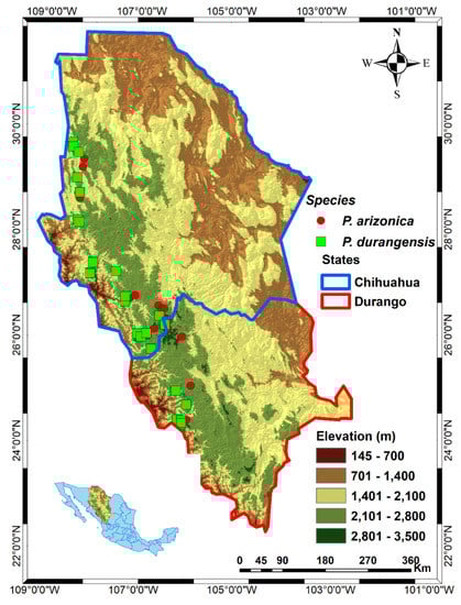
Figure 1.
Location of the studied populations of Pinus arizonica and P. durangensis in the states of Chihuahua and Durango, northwestern México.
2.2. Determination of Climate Variables
An already existing climate model [26] was used to extract 22 climate variables for each seed stand. This model is based on the Thin Plate Spline (TPS) method [27] implemented for Mexico [28], and estimates standardized monthly average values of minimum and maximum temperatures and precipitation, based on more than 200 climatic stations in Chihuahua and Durango, for the period 1961–1990 (Table S1). Point estimates for each location were obtained from a public database (available online: http://forest.moscowfsl.wsu.edu/climate/ (accessed on 10 December 2020)) by inputting geographic coordinates (latitude, longitude, and elevation).
2.3. Determination of Soil Variables
Soil subsamples were collected at a depth of 0–15 cm at the base of each of studied tree. Subsamples were combined in a composite sample (1 kg) per stand (50 samples in total), which was assumed to be representative of the soil of each entire stand. The following edaphic variables were determined: texture (relative proportion of clay, silt and sand), density (DEN, g/cm3), pH, and potassium (K, ppm), magnesium (Mg, ppm), sodium (Na, ppm), copper (Cu, ppm), iron (Fe, ppm), manganese (Mn, ppm), zinc (Zn, ppm) and calcium concentrations (Ca, ppm), which were measured according to Castellanos et al. [29]. Furthermore, phosphorus (P) concentration (ppm) was determined as in Olsen et al. [30], and nitrate amounts (NO3, kg/ha) were determined following Baker et al. [31] The relative content of organic matter (OM, %) was measured as in León and Aguilar, [32], and electrical conductivity (CE, dS/m) was determined according to Vázquez and Bautista, [33]. Cation exchange capacity (CEC, meq 100 g soil), the relative proportions (%) of hydrogen, CaCEC, MgCEC, KCEC, NaCEC and “other bases” (OB) were determined with the ammonium acetate method (pH 8.5) [34]. Finally, hydraulic conductivity (HC, CM/h) was determined following Mualem [35], and saturation percentage (SAT, %) according to Herbert [36]. Mean values per stand are available in Table S2.
2.4. Cluster Analysis
To detect the number of environmentally homogeneous seed stand clusters, we used the Affinity Propagation (AP) clustering technique, using the quantile (q) of input similarities [37]. This method includes all data points as potential “exemplars”. Furthermore, AP has several advantages over related techniques, such as k-centres clustering, the expectation maximization (EM) algorithm, Markov chain Monte Carlo procedures, hierarchical clustering and spectral clustering (see details in [38]). More importantly, a pre-defined number of groups is not needed [37]. For all the 25 seed stands per tree species, the AP was applied to all the climate and soil variables together (Tables S1 and S2). All analyses were implemented using the “apcluster” package for R [37].
2.5. Genetic Analysis
DNA data from the 35 needle samples per stand were analyzed using the AFLP technique, according to the protocol described by Vos et al. [39] and modified by Ávila-Flores et al. [40]. DNA was extracted using the QIAGEN DNeasy96 Plant Kit (Qiagen, Venlo, The Netherlands), and digested with restriction enzymes MseI and EcoRI. PCR amplification was carried out with double strands MseI and EcoRI adaptors, to bind to the end of the restriction fragments and produce DNA templates. Pre-amplification used the E01/M03 (EcoRI-A/MseI-G) primer combination, and selective amplification E35 primers (fluorescently marked with FAM) and M63 + C (MseI-GAAC), for both species. All PCR reactions were performed in a Peltier ThermoCycler (PTC-200 version 4.0, MJ Research, St. Bruno, Quebec, Canada). Products were electrophoresed in a genetic analyzer (ABI 3100 16 capillaries) together with an internal size standard (ROX fluorescent dye GeneScan 500 ROX from Applied Biosystems, Foster City, CA, USA). AFLP fragments were measured with GeneScan 3.7 and Genotyper 3.7 packages (Applied Biosystems) after confirming quality and reproducibility by using 16 randomly selected reference samples, which were duplicated within plates in independent analysis (PCR replicates). Only those peaks observed in replicated samples were retained [40,41]. Markers were coded in a binary matrix as presence (code 1) or absence (code 0) of specific peaks [42,43].
2.6. Outlier Detection
Outlier loci were identified with BayeScan v 2.1 [44,45], which is a software based on the multinomial Dirichlet model and uses the Jump Markov Chain Monte Carlo Reversible algorithm (RJMCMC) to obtain the posterior distributions. Inbreeding coefficients (FIS) used to estimate allele frequencies were not able to be estimated from binary data as purely dominant AFLP markers [46]. In BayeScan, FIS moves freely within its prior range in order to incorporate the uncertainty associated with FIS. A positive value of the locus-specific component (α) and a posterior probability >0.99 indicate differential selection (false discovery rates < 0.01), whereas negative α values with posterior probabilities >0.99 indicate possible balancing or purifying selection [45,47]. The following parameters were used: output number of iterations (5000), thinning interval size (10), pilot runs (20), length of pilot runs (5000), burn in (50,000), prior odds for the neutral model (10), lower boundary for uniform prior on the inbreeding coefficients FIS (0) and the upper boundary for uniform prior on FIS (1).
In addition, genetic differentiation (δ) among populations and Dj components for each AFLP locus [48] were used to identify loci putatively under differential selection. The non-parametric measure δ has various conceptually desirable properties and is based on the genetic distance (d0) [49], measured as the genetic difference between two biological collectives through pairwise comparison of genotypes, with a value of zero indicating genetically identical collectives, and a value of one completely different stands. Consequently, if the observed δ is smaller than 99.99% of the expected δ (i.e., p < 0.0001), the existence of non-random homogenizing forces (i.e., gene flow, balancing selection) is suspected, but if the observed δ is higher than 99.99% of the expected δ (i.e., p > 0.0001), non-random diversifying forces (differential selection or non-recurrent mutation) are inferred (see [48,50]). δ and its p value were calculated in GSED 3.0 ([51]; Available online: http://www.uni-goettingen.de/forstgenetik/gsed (accessed on 6 June 2020)) and checked in the self-written C program “Delta” in Linux).
2.7. Determination of AFLP Diversity
We analysed the genetic diversity of each seed stand through the mean genetic diversity (dg [23]), the proportion of polymorphic fragments (prpoly) and the DW index (which quantifies rare markers within cohorts). This last index is the sum of the proportion of occurrence of each marker per stand divided by the number of occurrences of the same marker in all the stands together. DW values are expected to be high when rare markers are accumulated within a stand [52]. The median values of dg, prpoly and DW observed in seed stand clusters which grow in similar environmental conditions, were compared with the overall median dg, prpoly and DW of the 25 seed stands together per tree species. It has been reported that differential selection caused by environmental conditions reduces genetic diversity [48]. Therefore, if differential selection occurs in a given cluster, the overall genetic diversity is expected to be higher.
2.8. Analysis of Molecular Variance and of Linkage Disequilibrium
To detect genetic differentiation between clusters, we further performed a hierarchical Analysis of Molecular Variance (AMOVA) [53] with GenAlEx 6.5 using 9999 permutations. Such differentiation was determined using the phiPT value (an analogue of the fixation index, FST) which allows for suppressing the within-cluster variance.
Natural selection, supporting adaptation to local environmental conditions, will increase overall linkage disequilibrium (LD) caused by differences in allele frequencies among subpopulations whenever alleles at different loci are favored. According to [54], the F statistic, when partitioning overall LD, is appropriate when trying to determine whether differences in LD result only from differences in allele frequency or from other factors, such as selection, that differ among populations [55,56,57].
In order to detect signs of possible selection, observed linkages among AFLP against expected distributions from permutation were evaluated using the standardized index of association ( [58]. This index corresponds to the corrected (standardized) difference of the observed variance (as the sum of the individual variances of the AFLP) divided by the expected variance (as the sum of all the variances over all the AFLP together). accounts for the number of AFLP sampled, which is less biased when calculated with the “poppr” package [59] in R and the p value is evaluated with 999 and 9999 permutations. “poppr” was created to perform analysis of populations with mixed reproductive patterns and allows analyzing haploid and diploid dominant/co-dominant marker data, including also AFLP. was calculated among all the AFLP, excepting all the outliers (i.e., only the putatively neutral AFLP) within each cluster of seed stands growing in similar environmental conditions and also for the whole sample of trees together (i.e., the overall ).
If differential selection occurs, the overall value is expected to be significantly higher (p < 0.01) when using only the outlier AFLP found, than the values among each cluster of seed stands growing in similar environmental conditions when using all the AFLP without outliers (i.e., putatively neutral AFLP). Such difference was verified with a non-parametric Kruskal–Wallis test [60] in R (version 4.0.2).
2.9. Modelling Seed Zones from Environmentally-Associated AFLP Variants and Environmental Factors
To evaluate the ability of climate, soil and geographic variables to explain the variation of outlier loci per species, we applied a multi-tiered variance partitioning method (e.g., [61]) to the results of a redundancy analysis (RDA) after including the Hellinger’s transformation, as implemented in the vegan R package (rda and varpart functions) [62,63].
We then evaluated the relationships between the relative frequencies (fr) of each outlier locus and the climate, soil and geographical variables of each species through covariance coefficients (C) with their respective p (Z ≥ C) values [48]. Since those variables are mostly nonlinear, we used methods that detect monotonous, but not necessarily linear, covariation. C allows for such a detection, where values close to 1 indicate highly positive covariation and those close to −1 a strictly negative covariation. C was calculated as:
where C = Covariation between each genetic variant at an outlier locus at the species X and each variable Y in the study sites. (Xi − Xj) = difference in the genetic variant values of each studied species X, between the i-th and the j-th loci. (Yi − Yj) = difference in value of the variable Y, between the i-th and j-th studied stands. The denominator of Equation (1) is the sum of absolute values of the products indicated.
We selected no-collinear environmental variables (|r| < 0.7) that were significantly correlated to the relative frequency (fr) of outlier loci (C) for modelling six species-specific machine learning algorithms (MLM) of fr, all including cross-validation (CV). We used the following methods: (i) linear regression (“lm”), (ii) Random Forest (“rf”), (iii) Neural Network (“nnet”), iv) Model Averaged Neural Network (“avNNet”), (v) Multi-Layer Perceptron (“mlpWeightDecay”) and (vi) Bayesian Regularized Neural Networks (“brnn”) [64,65] (Available online: http://topepo.github.io/caret/index.html (accessed on December 2020)) in R (version 3.3.4) [63] (see more in [11]). Models were tested 15 through 10-fold cross-validation, by using 80% of the dataset as a training set and the remaining 20% as a test set. The maximum number of variables per model was determined by the rule of ten events per variable [66,67], i.e., two selected variables for P. arizonica and two for P. durangensis with 25 stands (repetitions). We evaluated the goodness-of-fit of the regression using the (pseudo) coefficient of determination (R2), the root mean square error (RMSE) and mean squared error (MSE). The associations between fr and important environmental variables were represented graphically using the “ggplot2” package and the function (method = ‘gam’), for generalized additive models (GAM) [68] in R (version 3.3.4) [63].
2.10. Species Distribution Models
Species distribution models (SDM) were generated using the selected climate, soil, geographical and topographical variables. Random forest classification (RF) [69] was used to calculate, map and delineate each defined seed zone and its potential shift. We used the geographical coordinates of presence-absence points (for P. arizonica 615 presence and 4473 absence locations, and for P. durangensis 1119 presence and 3757 absence locations) to project the distribution depending on climate, soil, geographical and topographical variables in the study area. Climate data were obtained at a 30-arc second resolution (about 800 m) from the WorldClim database (Available online: https://worldclim.org/data/bioclim.html (accessed on 13 December 2020)). Models were initially generated for the 1960–1990 period, and then projected to the year 2030, according to a future emission scenario: RCP ~ 4.5 Wm−2, or approximately 650 ppm of CO2-equivalent in the year 2100 (Tables S5 and S8). In the A1FI and A2 scenarios, Houghton et al. [70] predicted 449 and 444 ppm for 2030. This early-future climate scenario was chosen to better verify the models, and also given the lack of other available climate models that predict low CO2 concentrations. We obtained soil variables from Available online: https://soilgrids.org/ (accessed on 13 December 2020)) (Tables S7 and S10), and the topographical data from a digital elevation model of INEGI (Available online: https://www.inegi.org.mx/ (accessed on 25 November 2020)) (Tables S6 and S9).
Using the Waikato Environment for Knowledge Analysis (WEKA) open source software [71], the potentially most important regressor variables were selected by the Wrapper method [72] to fit the random forest (RF) algorithm. We used a 10-fold cross validation approach, repeated 10 times [73,74]. The final presence–absence models were applied to environmentally spatial variables, which were resampled to a 30 arc-seconds resolution, to generate spatially continuous maps. The predictive ability of the RF model was further evaluated by the True Skill Statistic (TSS) [75], using WEKA (for more details, see [76]. The TSS (also known as the Hanssen–Kuipers discriminant) is an appropriate alternative to the area under a Receiver Operating Characteristic (ROC) Curve (AUC; [77]) in cases where model predictions are formulated as presence–absence models. The TSS accounts for both omission and commission errors and is not affected by the sample size of each class. The TSS is defined as sensitivity + specificity, and ranges from −1 to +1, where +1 indicates a perfect classification model and TSS values of zero or less indicate model performance no better than random [75,78].
The Matthews correlation coefficient (MCC) was also calculated, which is reported as a more informative and truthful score for evaluating binary classifications than accuracy (ratio between the number of correctly classified samples and the overall number of samples) [79]. We calculated the threshold of probability of presence (PoP) using the average PoP value that maximized the sum of sensitivity and specificity, and the PoP value that minimized the difference between the absolute values of sensitivity and specificity. The intuitive, and most commonly used, threshold of 0.5 may actually not be the threshold above which the species is most likely to be present [80].
Although adaptation is expected to vary clinally across the landscape [7], we created fixed-boundary zones. As survey data of spatial soil variables correlated with fr are not available, two seed zones per AFLP were classified and mapped, one zone including the dominant climatically AFLP variant (fr ≥ 0.5) and the other including the recessive variant (fr < 0.5). Thus, for more climatically-associated and edaphically-associated AFLP, the resolution of mosaic seed zone classes will be finer (2n AFLP zones). The SDMs included seed zones that were mapped and for which their size could be calculated.
Finally, SDMs built for 1990 and 2030 were compared with current data (2017–2019), available from forest resources management programs for four regions (UMAFORES 0802, 1001, 1005 and 1010) ([81,82,83], Unión de Permisionarios de la Unidad de Administración Forestal La Flor Durango A.C. 2019 and Unidad de Administración Forestal Santiago Papasquiaro A.C. 2019). These programs are based on forest inventories conducted in northern, central and southern locations of the geographical distribution of both species.
3. Results
3.1. Amount and Distribution of Genetic Diversity, AMOVA and Linkage Disequilibrium
We identified 371 polymorphic bands between 75 and 450 base-pairs long for Pinus arizonica and 369 for P. durangensis. Outlier analysis pinpointed 11.1% of these bands in P. arizonica and 12.5% in P. durangensis (Table S4).
Based on 46 environmental variables, the Affinity Propagation (AP) clustering technique detected three environmentally homogeneous seed stand clusters for the two pine species studied. In P. arizonica, the first cluster included seven seed stands (1, 3, 4, 6, 9, 14 and 17), the second cluster 12 seed stands (5, 7, 8, 10, 11, 15, 16, 19, 20, 23, 24 and 25) and the third, six seed stands (2, 12, 13, 18, 21 and 22) (Figure S6). With regard to P. durangensis, the seed stands were divided up into a cluster including 14 seed stands (1, 2, 3, 5, 6, 7, 9, 15, 16, 18, 19, 20, 24 and 25), a second cluster with six seed stands (4, 11, 12, 13, 14 and 21) and a third cluster with five seed stands (8, 10, 17, 22 and 23) (Figure S7).
The overall genetic diversity was not significantly higher than the median genetic diversity among the clusters of seed stands separated by climate, topographical and soil variables; either using all AFLP together or using only the outlier loci. However, AMOVA and LD estimates support the occurrence of selection signs in these three environmentally determined seed stand clusters. For each species, the AMOVA shows that the most differentiated clusters (Cluster 2 for P. arizonica and Cluster 3 for P. durangensis) responding to climatic and edaphic conditions were also the most genetically differentiated. Besides, the overall value using the outliers AFLP was significantly higher than the average among clusters (p < 0.05) (Tables S14–S24 and Figures S9 and S10).
3.2. Modelling Seed Zones through Environmentally Associated Variants
For P. arizonica and using all 42 outliers, the redundancy analysis revealed that the edaphological, climate and geographic variables explained 18.7% (p = 0.003) of the total variation of the retained outliers. The climatic variables proved most suitable for predicting the relative frequency of outliers (14.4%, p = 0.01), followed by soil variables (5.5%, p = 0.04). Climate variables further showed the largest independent effect (13.2%, p = 0.02) on the variation of outliers, again followed by the edaphological variables (4.2%, p = 0.06) (Figure 2, Table S12). On the other hand, the redundancy analysis for P. durangensis did not reveal any significant relationships for any group of variables (edaphological, climate or geographical) for explaining variation using all 47 outliers.
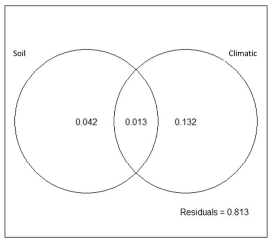
Figure 2.
Redundancy analysis and partition of variance for soil and climatic variables, for Pinus arizonica at northwestern Mexico. Results for P. durangensis were all non-significant and are not shown.
Using individual outlier loci, we observed four moderate but significant (p < 0.001) positive covariations between the relative frequency of some outliers (209, 314, 349 and 351) in P. arizonica and soil phosphorus concentration (P) and spring precipitation (SPRP; Table 1). For P. durangensis, two significantly negative and moderate covariations were detected (C = −0.91 and −0.81; p < 0.001) for the relative frequency of two outliers (240 and 416 frAFLP) with WINP and LAT, and positive covariations were observed for four other markers (236, 406, 416 and 342) and SPRP, MTWM, latitude and aridity index (AAI; Table 1).

Table 1.
Significant covariations (C[frAFLP × var]) found between relative AFLP variant frequencies (frAFLP) in Pinus arizonica and P. durangensis and various environmental variables (var). Outlier loci for each AFLP were detected from different selection models.
For P. durangensis, the best models included variables WINP, SPRP, LAT and AAI for predicting the frequency of AFLP variants 236, 240, 342, 406 and 416. Regarding P. arizonica, the best model for environmentally associated AFLP included phosphorous as a predictive variable. Figure 3 graphically represents the association between marker frequency and several predictor variables, for selected results from Table 1.
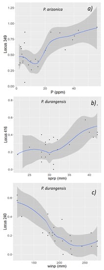
Figure 3.
Relationship between significant environmental variables and the relative frequency of selected AFLP outliers for Pinus arizonica (a) and P. durangensis (b,c), the mean (blue line) and standard deviation (grey area) are based on generalized additive models (GAM).
3.3. Species Distribution and Seed Zone Models for Pinus arizonica and P. durangensis
The best species distribution (SDM) models for P. arizonica and P. durangensis for the two-time frames considered (1961–1990 and 1990–2030; RCP ~ 4.5 Wm−2) were respectively elaborated with 18 and 21 independent environmental variables (Figure 4 and Figure 5, Figures S1–S3 and Tables S5–S10).
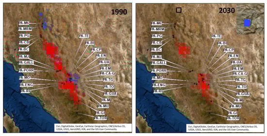
Figure 4.
Projection for 1990 and 2030 climatic frames of two seed zones of Pinus arizonica based on the relative frequency distribution of AFLP outlier 351; modelling based on spring precipitation (mm) (see Table 1). The species distribution was modeled by 18 environmental variables and the Random Forest classifier (Tables S5, S6 and S7a,b); the threshold for probability of presence (PoP) was 0.30; black points = P. arizonica seed stands studied here (Table S3a); blue color = relative frequency of the AFLP outlier locus 351 between 0.0 and 0.50; and red color = relative frequency of the AFLP outlier locus 351 between 0.51 and 1.0.
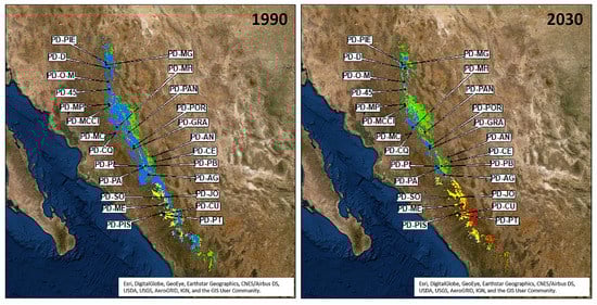
Figure 5.
Projection of seed zones distribution for Pinus durangensis for 1990 and 2030 climatic frames, based on the relative frequency of AFLP outliers (240 and 416); modelling based on spring and winter precipitation (mm) (see Table 1); the species distribution was modeled by 21 environmental variables using the Random Forest classifier (Tables S8, S9 and S10a,b). The threshold for probability of presence (PoP) was 0.35; black points = P. durangensis seed stands studied (Table S3b); green color = relative frequency of the adaptive AFLP-240 assumption between 0 and 0.50; red color = relative frequency of the adaptive AFLP-240 assumption between 0.51 and 1; blue color = relative frequency of the AFLP outlier locus 416 assumption between 0 and 0.50; and yellow color = relative frequency of the AFLP outlier locus 416 assumption between 0.51 and 1.
The most important variables for projecting P. arizonica distribution were the mean temperature of the warmest quarter, the precipitation in the driest month, the temperature seasonality, the mean temperature in the coldest quarter, and the mean diurnal range of temperature. For P. durangensis, the most important variables were precipitation in the driest quarter, soil pH, the mean temperature in the driest quarter, bulk density, and temperature seasonality (Tables S5–S10 and Figures S4 and S5). Relatively good validation statistics were obtained for both species’ models, with AUCs of 0.92. However, the TSS only showed values of 0.41 and 0.59 for P. arizonica and P. durangensis, respectively (Table 2).
Table 2.
Model fit metrics for the Pinus distribution models (SDM) estimated with Random Forest. Model fit was assessed both on training data used to fit the model and on the withheld test data used for model validation (5-fold).
Two seed zones were defined for P. arizonica based on the 1990 projection (Figure 4), which were defined by the relative frequency of AFLP 351 (fr) (>0.5 and ≤0.5) modelled against spring precipitation (Table 1). The seed zone for the major allele (fr > 0.5; shown in red in Figure 4) covered an area of about 1,859,761 ha (and included all seed stands studied), and the second seed zone, which mostly accounts variation of the minor allele (fr ≤ 0.5; shown in blue in Figure 4), covers an area of about 371,579 ha (modelled total P. arizonica distribution of 1,200,348 ha in 2019). Projections into 2030 (RCP 4.5) indicated a 56.5% expansion of the first seed zone (fr > 0.5; shown in red) accompanied by a shift of 18.4 km to the southwest. The second seed zone (fr ≤ 0.5; shown in blue) is expected to be reduced by 99.7%, and move 242 km to the northwest. According to this model P. arizonica would have lost some 35,551 ha annually between 1990 and 2030, shifting 31 km southwards and climbing 156 m to higher elevations (Figure 4, Table 3).
For P. durangensis, four seed zones were identified; these were based on the distribution of markers 240 and 416 modelled against spring and winter precipitation (SPRP and WINP) (Table 1). The first seed zone (red) covered an area 11,723 ha, the second one (yellow) an area of 347,708 ha, the third one (green) spanned over 790,409 ha (and included seed stands PD-AN, PD-CE and PD-PB), and the fourth one (blue) covered an area of 2,254,168 ha. Thus, the total modelled area for this species was 3,404,008 ha in climatic conditions of 1990 (Figure 5).
The size and position of all P. durangensis seed zones will change by 2030. The first seed zone (red in Figure 5) will expand 309 ha and move 56 km to the northwest; the second zone (yellow in Figure 5) will expand to an area of 482,322 ha and move 67 km to the northwest; the third zone (green) will also expand until reaching an area of 1,056,237 ha and will shift 105 km to the northwest. Finally, the fourth zone (blue) will decline by 25.4% and move 100 km to the northwest. The total distribution of P. durangensis will therefore decrease by 24,579 ha between 1990 and 2030 (RCP ~ 4.5 Wm−2). The model also indicates an average distribution shift of 9 km to the northwest and a mean elevation increase of 43 m in the same period (Figure 4, Table 3 and Table S13).
4. Discussion
4.1. AFLP-Environment Associations
In this study, we found that seed stands growing in similar climate-soil conditions are genetically similar, either using all AFLP or only using the outlier loci (Tables S14–S21). However, the genetic diversity was similar among the three environmentally homogeneous seed stand clusters, probably caused by: (i) the large populations with high gene flow and small gene drift and similar selection degree [84] in which the seed stands grow and (ii) using all (mostly neutral) AFLP. The redundancy analysis model (RDA) for P. arizonica showed that the explained outlier variance was especially associated with climate (Figure 2 and Table S12). Higher proportions of the environmental-associated variance were also explained in similar studies with other species. For instance, Capblancq et al. [85] reported that 35.2% of the variance was explained by climate variables in a study on Fagus sylvatica involving 36 locations, 570 trees and 65 outlier SNPs. Cullingham et al. [86] reported 27.3% of the variance was explained by climate variables, in a study of Pinus contorta, based on 36 localities. However, in a study of Quercus lobata involving 13 locations, 45 trees and 195 SNPs, Sork et al. [87] found that only 6% of the total variation was explained by climate variables. All of these studies also reported higher proportions of explained variance, of respectively 47%, 15% and 68%. However, none of the studies included soil variation, which in our case accounted for up to 5.5% of the explained environmental-associated variance (Figure 2 and Table S12). A similar result was observed for Quercus liaotungensis [88].
Some outlier loci were significantly associated with climate, edaphic and geographical variables, especially spring and winter precipitation, and phosphorus (P) concentration in the soil (Table 1 and Figure 3). Previous studies on plant species have reported correlations between both climate (rainfall/temperature) and geographical variables and outlier loci [89,90,91,92,93,94]. Temperature-linked spatial and temporal trends in AFLP frequency have also been reported for Fagus sylvatica L. [90], in which an association between AFLP and genecological prediction including 35 climate variables was observed. However, plant studies involving relationships between AFLP and soil traits are scarce; one of the few studies on this topic was presented by Quintela-Sabarís et al. [95], who reported associations between AFLP and the Mn and Sb total soil content in Cistus ladanifer L. Soil-associated AFLP differentiation has also been observed in Picea chihuahuana M. and attributed to different copper concentrations in the topsoil [96].
Phosphorus is a vital macronutrient for plant growth and development. Various genes confer adaptation to inorganic P, mainly by regulating P acquisition, internal remobilization, metabolic changes and signal transduction [97,98].
In the present study, the regression models for the relative frequency of some outlier loci by AFLP showed a similar fit for some soil and climate variables, also confirmed by the root-mean-square error (0.13–0.18 for the P concentration in the soil and 0.09–0.15 for climate variables) and the cross-valuated pseudo R2 (0.45–0.62 for P in the soil and 0.30–0.69 for climate variables) (Table 1 and Figure 3). The mean differences between extreme AFLP frequencies were 0.71 (range 0–0.71) and 0.74 (range 0–0.74) for the winter and the spring precipitation gradients, respectively (Table S11). Hornoy et al. [99] reported RF regression models of SNP allele frequency in Picea glauca with climatic gradients using 46 SNPs (from 11,085 SNPs) of those most strongly associated with climate, reaching a plateau at around 10 SNPs (pseudo R2 = 0.50–0.55); the same authors found that the mean differences between extreme SNP allele frequencies were 0.31 ± 0.08 (range 0.04–0.46, n = 39) and 0.32 ± 0.08 (range 0.21–0.47, n = 11) for the gradients of mean annual temperature and the total annual precipitation, respectively. Lotterhos et al. [100] found an association between each of 801 top candidate SNPs (out of 585,270 exome SNPs, n > 250) and 18 climate and three geographical variables (Spearman’s R2 ≤ 0.36). Therefore, our models relating AFLP frequencies and some environmental variables (Table 1) can be considered powerful enough to estimate the spatial distribution of some environmental-associated AFLP, in the two pine species under study. Joint analysis of the covariation, regression models (Table 1, Figure 3) and RDA (Figure 2) suggest that many outlier loci found were probably associated with other variables not included in our study. Sample size and design, marker type, and environmental cline can influence the detection of association of adaptive genetic traits with environmental variables [87].
4.2. Species Distribution and Seed Zones Models
Given the large number of climate, soil, geographical and topographical variables considered, and the many presence points and recognized statistical techniques [101,102] used to build our models, we were able to produce SDMs for both P. arizonica and P. durangensis supported by good validation statistics (AUC = 0.92) in comparison to other studies on tree species [101,103]. In contrast to Castellanos-Acuña et al. [7] and Shirk et al. [101], our study showed that shifts in species and seed zones distribution may take place from the southeast to the northwestern of the Sierra Madre Occidental (Table 3) probably since these mountains run southeast–northwest.
Castellanos-Acuña et al. [7] determined the concept of global seed zones for the whole of Mexico, independently of tree species. However, our study indicated that both the pine species and their genetic variants studied, respectively, were environment-associated (Tables S5–S10, Table 2). Therefore, the seed zones must be delimited for specific species, in order to achieve higher rates of survival of future reforestations.
In this work, of the total AFLP outliers, we found only 4–5 AFLP which were significantly directly or indirectly associated with specific climate and soil variables (Table 1). Such a few loci are probably not enough to delimit seed zones, particularly as we have not performed studies on associations between individual fitness or population density and these markers’ frequencies. On the other hand, only one or a few mutations in a single gene can be sufficient to dramatically impact tree fitness. E.g., Liu et al. [104] found Pinus monticola pathogenesis-related gene PmPR10–2 alleles as defense candidates for stem quantitative disease resistance against white pine blister rust (Cronartium ribicola) often provoking a lethal infection. Likewise, Hernández-Velasco et al. [21] found strong significant association (R2 > 0.72, p < 0.00004) between seedlings’ growth traits which were growing in the same climate and soil conditions and mean annual precipitation, winter precipitation, mean annual temperature, length of the frost-free period and maximum temperature in the warmest month in 20 provenances of five Mexican pine species (including P. arizonica and P. durangensis). However, although it cannot be ruled out that there are other genetic evolutionary factors, as selection, leading to stronger AFLP differentiation in the genome, various studies have used only few AFLP outlier [45,105] to detect natural selection, adaptation and provenances regions (e.g., [89,106,107,108].
The 4.5 Wm−2 projections used for the period 1990–2030 predict higher temperatures [70] than are likely for this period resulting in smaller predicted distributions for both P. arizonica and P. durangensis than in reality. Our SDMs indicated that the species distributions were slightly larger in 2019 than in the corresponding forest management plans for the same year (Table 3), indicating that climate change between 1990 and 2019 (and 2030) can only partly explain the strong reductions of the species and seed zone distributions found in reality.
Thus, other factors such as forest fires, plagues, diseases, species over-exploitation, along with clearing to make room for pastures for grazing cattle may also contribute to reducing the species distributions. In this context, the main silvicultural system “Método Mexicano de Ordenación de Bosques Irregulares (MMOBI)”, applied to forest management in the Sierra Madre Occidental, is based on selective extraction still focused mainly on large trees, and relatively little attention is given to species composition in the natural regeneration [109,110]. This silvicultural system may therefore tend to over-exploit commercially attractive tree species, such as P. arizonica and P. durangensis, in the typically uneven-aged mixed pine-oak forests.
To reduce the over-exploitation of these two species, we recommend adapting or changing the current forest management system [111], making correct selections including different diameter categories of the trees to be harvested, conducting a strict, independent and professional state supervision and, promoting higher levels of forest knowledge [112]. Alternative regeneration methods, such as irregular group shelterwood (Expanding Gap Silviculture “Femelschlag”), should also be considered, in order to improve natural regeneration. Complementary reforestation and plantation with appropriate seeds, taking into account the optimal seed zones and their shifting, found in this study, may help enhance the regeneration of the forest [111].
5. Conclusions
In conclusion, this research shows that environmental and genetic traits may be useful to delimit seed zones. However, AFLP have limits when predicting local adaptation [43,113,114,115], especially if only a small number of populations and AFLP related to environmental variables are used. Therefore, our delimitation of proposed seed zones should be understood as a working hypothesis for subsequent studies. In order to find a better delimitation of seed zones, we recommend checking our results using genome-wide clearly adaptive molecular markers, such as SNP [1], paired with reciprocal provenance trials.
However, to restore populations of native tree species, seed collection limited to a very local area is commonly recommended. Given that adaptation is specific for the two economically important pine species studied and their seed zones included in this research, complementary studies are needed to evaluate the possible differences of using local versus non-local seeds. Consequently, more research on plant provenances and seed zones restoration is recommended, aiming to achieve best practices in forest restoration and conservation. Additionally, a reforestation guide taking into account the issue of the distribution reduction and the shifting of the studied species and their seed zones, could be helpful to improve forest management.
Supplementary Materials
The following are available online at https://www.mdpi.com/article/10.3390/f12050570/s1.
Author Contributions
C.W. conceived and designed the experiments and with S.L.S.-R. conducted sampling; S.L.S.-R., C.W. and C.A.L.-S. analysed the data and prepared figures and tables; C.W. contributed reagents/materials/analysis tools; all authors discussed the results; C.W. and S.L.S.-R. wrote the paper; S.L.S.-R., C.W., C.A.L.-S., J.P.J.-C., L.F.-R., A.P.-L., A.C.-P., J.C.H.-D. contributed to writing and reviewing drafts of the manuscript and to the final publication of the paper. All authors have read and agreed to the published version of the manuscript.
Funding
This research was funded by the Comisión Nacional Forestal and Consejo Nacional de Ciencia y Tecnología, Mexico.
Institutional Review Board Statement
Not applicable.
Informed Consent Statement
Not applicable.
Acknowledgments
We are grateful to UMAFOR La Flor 1010, Santiago 1005 and Madera 0802 for providing information of the management plans (used to validate our SMD). We thank Javier Hernández-Velasco and Carlos Alonso Reyes-Murillo for help in collecting samples and geographic data. We are also grateful to the Comisión Nacional Forestal (CONAFOR) for the financial support provided to C.W. and to Consejo Nacional de Ciencia y Tecnología (CONACYT) for the grants provided to S.L.S.-R. (CVU 479097) and A.P.-L.
Conflicts of Interest
C.W, and C.A.L.-S. are Academic Editors for Forests. The funders had no role in the design of the study; in the collection, analyses, or interpretation of data; in the writing of the manuscript, or in the decision to publish the results.
References
- De Kort, H.; Mergeay, J.; Vander Mijnsbrugge, K.; Decocq, G.; Maccherini, S.; Kehlet Bruun, H.H.; Honnay, O.; Vandepitte, K. An evaluation of seed zone delineation using phenotypic and population genomic data on black alder Alnus glutinosa. J. Appl. Ecol. 2014, 51, 1218–1227. [Google Scholar] [CrossRef]
- McKay, J.K.; Christian, C.E.; Harrison, S.; Rice, K.J. “How local is local?”—A review of practical and conceptual issues in the genetics of restoration. Restor. Ecol. 2005, 13, 432–440. [Google Scholar] [CrossRef]
- O’Brien, E.K.; Krauss, S.L. Testing the home-site advantage in forest trees on disturbed and undisturbed sites. Restor. Ecol. 2010, 18, 359–372. [Google Scholar] [CrossRef]
- St. Clair, J.B.; Howe, G.T.; Wright, J.; Becoin, R. Available online: https://www.fs.usda.gov/pnw/tools/center-forest-provenance-data (accessed on 24 June 2020).
- Ying, C.C.; Yanchuk, A.D. The development of British Columbia’s tree seed transfer guidelines: Purpose, concept, methodology, and implementation. For. Ecol. Manag. 2006, 227, 1–13. [Google Scholar] [CrossRef]
- Rehfeldt, G.E. Seed Transfer Guidelines for Douglas-Fir in Central Idaho; US Department of Agriculture, Forest Service, Intermountain Forest and Range Experiment Station: Odgen, UT, USA, 1983.
- Castellanos-Acuña, D.; Vance-Borland, K.W.; St. Clair, J.B.; Hamann, A.; López-Upton, J.; Gómez-Pineda, E.; Ortega-Rodríguez, J.M.; Sáenz-Romero, C. Climate-based seed zones for Mexico: Guiding reforestation under observed and projected climate change. New For. 2018, 49, 297–309. [Google Scholar] [CrossRef]
- Campbell, R. Soils, Seed-Zone Maps, and Physiography: Guidelines for Seed Transfer of Douglas-Fir in Southwestern Oregon. For. Sci. 1991. [Google Scholar] [CrossRef]
- Lindgren, D.; Ying, C.C. A model integrating seed source adaptation and seed use. New For. 2000, 20, 87–104. [Google Scholar] [CrossRef]
- Rehfeldt, G.E. Genetic variation, climate models and the ecological genetics of Larix occidentalis. For. Ecol. Manag. 1995, 78, 21–37. [Google Scholar] [CrossRef]
- Leal-Sáenz, A.; Waring, K.M.; Menon, M.; Cushman, S.A.; Eckert, A.; Flores-Rentería, L.; Hernández-Díaz, J.C.; López-Sánchez, C.A.; Martínez-Guerrero, J.H.; Wehenkel, C. Morphological Differences in Pinus strobiformis Across Latitudinal and Elevational Gradients. Front. Plant Sci. 2020, 11, 559697. [Google Scholar] [CrossRef]
- Hereford, J. A quantitative survey of local adaptation and fitness trade-offs. Am. Nat. 2009, 173, 579–588. [Google Scholar] [CrossRef]
- Ghalambor, C.K.; McKay, J.K.; Carroll, S.P.; Reznick, D.N. Adaptive versus non-adaptive phenotypic plasticity and the potential for contemporary adaptation in new environments. Funct. Ecol. 2007, 21, 394–407. [Google Scholar] [CrossRef]
- Krauss, S.L.; Sinclair, E.A.; Bussell, J.D.; Hobbs, R.J. An ecological genetic delineation of local seed-source provenance for ecological restoration. Ecol. Evol. 2013, 3, 2138–2149. [Google Scholar] [CrossRef]
- Hodge, G.R.; Dvorak, W.S. Breeding southern US and Mexican pines for increased value in a changing world. New For. 2014, 45, 295–300. [Google Scholar] [CrossRef]
- CONAFOR Establecimiento de Unidades Productoras y Manejo de Germoplasma Forestal-Especiaciones Técnicas; Declaratoria de Vigencia de la Norma Mexicana NMX-AA-169-SCFI-2014; Diario Oficial de la Federación: México City, Mexico, 2014.
- Villaseñor, J.L. Informe Final* del Proyecto JE012 La flora arbórea de México. Available online: www.conabio.gob.mx (accessed on 25 April 2013).
- Hernández-León, S.; Gernandt, D.S.; Pérez de la Rosa, J.A.; Jardón-Barbolla, L. Phylogenetic Relationships and Species Delimitation in Pinus Section Trifoliae Inferrred from Plastid DNA. PLoS ONE 2013, 8, e70501. [Google Scholar] [CrossRef]
- Bustamante-García, V.; Prieto-Ruíz, J.Á.; Merlín-Bermudes, E.; Álvarez-Zagoya, R.; Carrillo-Parra, A.; Hernández-Díaz, J.C. Potencial y eficiencia de producción de semilla de Pinus engelmannii Carr.; en tres rodales semilleros del estado de Durango, México. Madera y Bosques 2012, 18, 7–21. [Google Scholar] [CrossRef]
- Ramos-Ramírez, E. Viabilidad de Semillas en diez Especies de Pinus Procedentes de Rodales Semilleros Ubicados en el Estado de Durango; Universidad Juárez del Estado de Durango: Durango, México, 2019. [Google Scholar]
- Hernández-Velasco, J.; Hernández-Díaz, J.C.; Vargas-Hernández, J.; Hipkins, V.; Prieto-Ruíz, J.Á.; Pérez-Luna, A.; Wehenkel, C. Hybrid vigor in natural seed stands of seven Mexican Pinus species. New For. 2021. under review. [Google Scholar]
- Friedrich, S.C.; Hernández-Díaz, J.C.; Leinemann, L.; Prieto-Ruíz, J.A.; Wehenkel, C. Spatial genetic structure in seed stands of Pinus arizonica Engelm. and Pinus cooperi blanco in the state of Durango, Mexico. For. Sci. 2018, 64, 191–202. [Google Scholar] [CrossRef]
- Hill, M.O. Diversity and Evenness: A Unifying Notation and Its Consequences. Ecology 1973, 54, 427–432. [Google Scholar] [CrossRef]
- Hernández-Velasco, J.; Hernández-Díaz, J.C.; Fladung, M.; Cañadas-López, Á.; Prieto-Ruíz, J.Á.; Wehenkel, C. Spatial genetic structure in four Pinus species in the Sierra Madre Occidental Durango, Mexico. Can. J. For. Res. 2017, 47, 73–80. [Google Scholar] [CrossRef]
- Wehenkel, C.; Simental-Rodríguez, S.L.; Silva-Flores, R.; Hernández-Díaz, J.C.; López-Sánchez, C.A.; Martínez-Antúnez, P. Unterscheidung von 59 Saatgutbeständen verschiedener mexikanischer Kiefernarten anhand von 43 dendrometrischen, klimatischen, edaphischen und genetischen Variablen. Forstarchiv 2015. [Google Scholar] [CrossRef]
- Rehfeldt, G.E. A Spline Model of Climate for the Western United States; Gen. Tech. Rep. RMRS-GTR-165; US Department of Agriculture, Forest Service, Rocky Mountain Research Station: Fort Collins, CO, USA, 2006.
- Hutchinson, M.F. Continent-wide data assimilation using thin plate smoothing splines. Data Assim. Syst. Bureau Meteorol. Melb. 1991, 104–113. [Google Scholar]
- Sáenz-Romero, C.; Rehfeldt, G.E.; Crookston, N.L.; Duval, P.; St-Amant, R.; Beaulieu, J.; Richardson, B.A. Spline models of contemporary, 2030, 2060 and 2090 climates for Mexico and their use in understanding climate-change impacts on the vegetation. Clim. Chang. 2010, 102, 595–623. [Google Scholar] [CrossRef]
- Castellanos, J.Z.; Uvalle-Bueno, J.X.; Aguilar-Santelises, A. Manual de Interpretación de Análisis de Suelos y Aguas Agrícolas, Plantas y ECP., 2nd ed.; Instituto de Capacitación para la Productividad Agrícola: Ciudad de México, México, 1999; p. 201. [Google Scholar]
- Olsen, S.R. Estimation of Available Phosphorus in Soils by Extraction with Sodium Bicarbonate; US Department of Agriculture: Washington, DC, USA, 1954.
- Baker, A.S. Colorimetric Determination of Nitrate in Soil and Plant Extracts with Brucine. J. Agric. Food Chem. 1967, 15, 802–806. [Google Scholar] [CrossRef]
- León-Arteta, R.; Aguilar-Santelises, A.; Etchevers-Barra, J.D.; Castellanos, J.Z. 1987 Materia orgánica. Análisis Químico para Evaluar la Fertilidad del Suelo. Soc. Mex. la Cienc. del Suelo 1987, 85–91. [Google Scholar]
- Vázquez, A.A.; Bautista, N. Guía Para Interpretar El Análisis Químico de Suelo y Agua. 1993. Available online: https://www.mapa.gob.es/ministerio/pags/biblioteca/hojas/hd_1993_05.pdf (accessed on 25 March 2021).
- Normandin, V.; Kotuby-Amacher, J.; Miller, R.O. Modification of the ammonium acetate extractant for the determination of exchangeable cations in calcareous soils. Commun. Soil Sci. Plant Anal. 1998, 29, 1785–1791. [Google Scholar] [CrossRef]
- Mualem, Y. A new model for predicting the hydraulic conductivity of unsaturated porous media. Water Resour. Res. 1976, 12, 513–522. [Google Scholar] [CrossRef]
- Valle, F.H.D.; Herbert, V.F. Prácticas de Relaciones Agua-Suelo-Planta-Atmósfera; Universidad Autónoma de Chapingo: Chapingo, México, 1992; Volume 3, p. 167. [Google Scholar]
- Bodenhofer, U.; Kothmeier, A.; Hochreiter, S. Apcluster: An R package for affinity propagation clustering. Bioinformatics 2011, 27, 2463–2464. [Google Scholar] [CrossRef]
- Frey, B.J.; Dueck, D. Clustering by passing messages between data points. Science 2007, 315, 972–976. [Google Scholar] [CrossRef]
- Vos, P.; Hogers, R.; Bleeker, M.; Reijans, M.; Van De Lee, T.; Hornes, M.; Friters, A.; Pot, J.; Paleman, J.; Kuiper, M.; et al. AFLP: A new technique for DNA fingerprinting. Nucleic Acids Res. 1995, 23, 4407–4414. [Google Scholar] [CrossRef] [PubMed]
- Ávila-Flores, I.J.; Hernández-Díaz, J.C.; González-Elizondo, M.S.; Prieto-Ruíz, J.Á.; Wehenkel, C. Degree of hybridization in seed stands of Pinus engelmannii Carr. in the Sierra Madre Occidental, Durango, Mexico. PLoS ONE 2016, 11, e0152651. [Google Scholar] [CrossRef] [PubMed]
- Kuchma, O.; Vornam, B.; Finkeldey, R. Mutation rates in Scots pine (Pinus sylvestris L.) from the Chernobyl exclusion zone evaluated with amplified fragment-length polymorphisms (AFLPs) and microsatellite markers. Mutat. Res. Genet. Toxicol. Environ. Mutagen. 2011, 725, 29–35. [Google Scholar] [CrossRef]
- Krauss, S.L. Accurate gene diversity estimates from amplified fragment length polymorphism (AFLP) markers. Mol. Ecol. 2000, 9, 1241–1245. [Google Scholar] [CrossRef] [PubMed]
- Bonin, A.; Bellemain, E.; Bronken Eidesen, P.; Pompanon, F.; Brochmann, C.; Taberlet, P. How to track and assess genotyping errors in population genetics studies. Mol. Ecol. 2004, 13, 3261–3273. [Google Scholar] [CrossRef] [PubMed]
- Fischer, M.C.; Foll, M.; Excoffier, L.; Heckel, G. Enhanced AFLP genome scans detect local adaptation in high-altitude populations of a small rodent (Microtus arvalis). Mol. Ecol. 2011, 20, 1450–1462. [Google Scholar] [CrossRef]
- Foll, M.; Gaggiotti, O. A genome-scan method to identify selected loci appropriate for both dominant and codominant markers: A Bayesian perspective. Genetics 2008, 180, 977–993. [Google Scholar] [CrossRef] [PubMed]
- Simental-Rodríguez, S.L.; Quinones-Pérez, C.Z.; Moya, D.; Hernández-Tecles, E.; Lopez-Sanchez, C.A.; Wehenkel, C. The relationship between species diversity and genetic structure in the rare Picea Chihuahuana tree species community, Mexico. PLoS ONE 2014, 9, e111623. [Google Scholar] [CrossRef]
- Foll, M.; Fischer, M.C.; Heckel, G.; Excoffier, L. Estimating population structure from AFLP amplification intensity. Mol. Ecol. 2010, 19, 4638–4647. [Google Scholar] [CrossRef]
- Gregorius, H.R.; Degen, B.; König, A. Problems in the analysis of genetic differentiation among populations—A case study in Quercus robur. Silvae Genet. 2007, 56, 190–199. [Google Scholar] [CrossRef]
- Gregorius, H.R. On the concept of genetic distance between populations based on gene frequencies. In IUFRO Joint Meeting of Working Parties on Popul. and Ecol. Genet., Breed Theory and Progeny Testing; Elsevier: Stockholm, Sweden, 1974; pp. 413–438. [Google Scholar]
- Wehenkel, C.; Corral-Rivas, J.J.; Hernández-Díaz, J.C.; Von Gadow, K. Estimating balanced structure areas in multi-species forests on the Sierra Madre Occidental, Mexico. Ann. For. Sci. 2011, 68, 385–394. [Google Scholar] [CrossRef]
- Gillet, E.M.; Gregorius, H.R. Measuring differentiation among populations at different levels of genetic integration. BMC Genet. 2008, 9, 60. [Google Scholar] [CrossRef]
- Schönswetter, P.; Tribsch, A. Vicariance and dispersal in the alpine perennial Bupleurum stellatum L. (Apiaceae). Taxon 2005, 54, 725–732. [Google Scholar] [CrossRef]
- Excoffier, L.; Smouse, P.E.; Quattro, J.M. Analysis of molecular variance inferred from metric distances among DNA haplotypes: Application to human mitochondrial DNA restriction data. Genetics 1992. [Google Scholar] [CrossRef]
- Wright, S. Breeding Structure of Populations in Relation to Speciation. Am. Nat. 1940, 74, 232–248. [Google Scholar] [CrossRef]
- Ohta, T. Linkage disequilibrium due to random genetic drift in finite subdivided populations. Proc. Natl. Acad. Sci. USA 1982, 79, 1940–1944. [Google Scholar] [CrossRef]
- Ohta, T. Linkage disequilibrium with the island model. Genetics 1982, 101, 139–155. [Google Scholar] [CrossRef] [PubMed]
- Slatkin, M. Linkage disequilibrium—Understanding the evolutionary past and mapping the medical future. Nat. Rev. Genet. 2008, 9, 477–485. [Google Scholar] [CrossRef] [PubMed]
- Agapow, P.M.; Burt, A. Indices of multilocus linkage disequilibrium. Mol. Ecol. Notes 2001, 1, 101–102. [Google Scholar] [CrossRef]
- Kamvar, Z.N.; Tabima, J.F.; Grünwald, N.J. An R package for genetic analysis of populations with clonal, partially clonal, and/or sexual reproduction. PeerJ 2014, 2, e281. [Google Scholar] [CrossRef] [PubMed]
- Kruskal, W.H.; Wallis, W.A. Use of Ranks in One-Criterion Variance Analysis. J. Am. Stat. Assoc. 1952, 47, 583–621. [Google Scholar] [CrossRef]
- Cushman, S.A.; McGarigal, K. Hierarchical, multi-scale decomposition of species-environment relationships. Landsc. Ecol. 2002, 17, 637–646. [Google Scholar] [CrossRef]
- Oksanen, J.; Blanchet, F.G.; Kindt, R.; Legendre, P.; O’Hara, R.B.; Simpson, G.L.; Solymos, P.; Stevens, M.H.H.; Wagner, H. Vegan: Community Ecology Package, R Package Version 1.17-4; 2010. Available online: https://cran.r-project.org/web/packages/vegan/index.html (accessed on 25 March 2021).
- R Core Team. R: A Language and Environment for Statistical Computing; R Foundation for Statistical Computing: Vienna, Austria, 2017. [Google Scholar]
- Venables, W.N.; Ripley, B.D. Chapter 10: Tree-based methods. In Modern Applied Statistics with S-Plus, Statistics and Computing, 3rd ed.; Chambers, J., Eddy, W., Härdle, W., Sheather, S., Tierney, L., Eds.; Springer-Verlag Press: New York, NY, USA, 1999; pp. 303–327. [Google Scholar] [CrossRef]
- Williams, C.K.; Engelhardt, A.; Cooper, T.; Mayer, Z.; Ziem, A.; Scrucca, L.; Kuhn, M.M. Package ‘Caret’, Version 6.0-80 2018. Available online: https://cran.r-project.org/web/packages/caret/caret.pdf (accessed on 14 May 2020).
- McGarigal, K.; Stafford, S.; Cushman, S. Multivariate Statistics for Wildlife and Ecology Research; Springer: New York, NY, USA, 2000; p. 283. [Google Scholar]
- Vittinghoff, E.; McCulloch, C.E. Relaxing the rule of ten events per variable in logistic and cox regression. Am. J. Epidemiol. 2007, 165, 710–718. [Google Scholar] [CrossRef]
- Wickham, H. ggplot2: Elegant Graphics for Data Analysis; Springer-Verlag: New York, NY, USA, 2016; ISBN 978-3-319-24277-4. Available online: https://ggplot2.tidyverse.org (accessed on 25 March 2021).
- Breiman, L. Random forests. Mach. Learn. 2001, 45, 5–32. [Google Scholar] [CrossRef]
- Houghton, J.T.; Houghton, Y.D.J.G.; Ding, D.J.; Griggs, M.; Noguer, P.J.; van der Linden, X.; Dai, K.; Maskell, C.A.J. Climate Change. Sci. Basis 2001, 861–881. [Google Scholar]
- Hall, M.; Frank, E.; Holmes, G.; Pfahringer, B.; Reutemann, P.; Witten, I.H. The WEKA data mining software: An update. ACM SIGKDD Explor. Newsl. 2009, 11, 1–9. [Google Scholar] [CrossRef]
- Hall, M. Correlation-Based Feature Selection for Machine Learning; The University of Waikato: Hamilton, New Zealand, 1999. [Google Scholar]
- Deschamps, B.; McNairn, H.; Shang, J.; Jiao, X. Towards operational radar-only crop type classification: Comparison of a traditional decision tree with a random forest classifier. Can. J. Remote Sens. 2012, 38, 60–68. [Google Scholar] [CrossRef]
- Wang, L.; Zhou, X.; Zhu, X.; Dong, Z.; Guo, W. Estimation of biomass in wheat using random forest regression algorithm and remote sensing data. Crop J. 2016, 4, 212–219. [Google Scholar] [CrossRef]
- Allouche, O.; Tsoar, A.; Kadmon, R. Assessing the accuracy of species distribution models: Prevalence, kappa and the true skill statistic (TSS). J. Appl. Ecol. 2006, 43, 1223–1232. [Google Scholar] [CrossRef]
- Castaño-Santamaría, J.; López-Sánchez, C.A.; Ramón Obeso, J.; Barrio-Anta, M. Modelling and mapping beech forest distribution and site productivity under different climate change scenarios in the Cantabrian Range (North-western Spain). For. Ecol. Manag. 2019. [Google Scholar] [CrossRef]
- Fawcett, T. An introduction to ROC analysis. Pattern Recognit. Lett. 2006, 27, 861–874. [Google Scholar] [CrossRef]
- Tatler, J.; Cassey, P.; Prowse, T.A.A. High accuracy at low frequency: Detailed behavioural classification from accelerometer data. J. Exp. Biol. 2018, 221, jeb184085. [Google Scholar] [CrossRef]
- Chicco, D.; Jurman, G. The advantages of the Matthews correlation coefficient (MCC) over F1 score and accuracy in binary classification evaluation. BMC Genom. 2020. [Google Scholar] [CrossRef] [PubMed]
- Jiménez-Valverde, A.; Lobo, J.M. Threshold criteria for conversion of probability of species presence to either-or presence-absence. Acta Oecol. 2007, 31, 361–369. [Google Scholar] [CrossRef]
- Ramos, I.; (Unidad de Manejo Forestal 0802, Madera, Chihuahua, México); Bustillos, R.D.; (Unidad de Manejo Forestal 00802, Madera, Chihuahua, México); Martínez, C.L.; (Unidad de Manejo Forestal 0802, Madera, Chihuahua, México). Personal communication, 2020.
- Rodríguez, S.G.; (Unidad de Manejo Forestal 1001, Guanaceví, Durango, México). Personal communication, 2020.
- Rodríguez, S.G.; (Unidad de Manejo Forestal 0802, Madera, Chihuahua, México). Personal communication, 2020.
- Reed, D.H.; Frankham, R. Correlation between fitness and genetic diversity. Conserv. Biol. 2003, 17, 230–237. [Google Scholar] [CrossRef]
- Capblancq, T.; Morin, X.; Gueguen, M.; Renaud, J.; Lobreaux, S.; Bazin, E. Climate-associated genetic variation in Fagus sylvatica and potential responses to climate change in the French Alps. J. Evol. Biol. 2020, 33, 783–796. [Google Scholar] [CrossRef]
- Cullingham, C.I.; Cooke, J.E.K.; Coltman, D.W. Cross-species outlier detection reveals different evolutionary pressures between sister species. New Phytol. 2014, 204, 215–229. [Google Scholar] [CrossRef]
- Sork, V.L.; Fitz-Gibbon, S.T.; Puiu, D.; Crepeau, M.; Gugger, P.F.; Sherman, R.; Stevens, K.; Langley, C.H.; Pellegrini, M.; Salzberg, S.L. First draft assembly and annotation of the genome of a California endemic oak Quercus lobata Née (Fagaceae). G3 Genes Genomes Genet. 2016, 6, 3485–3495. [Google Scholar] [CrossRef]
- Yang, J.; Vázquez, L.; Feng, L.; Liu, Z.; Zhao, G. Climatic and soil factors shape the demographical history and genetic diversity of a deciduous oak (quercus liaotungensis) in Northern China. Front. Plant Sci. 2018. [Google Scholar] [CrossRef]
- Jump, A.S.; Hunt, J.M.; Martínez-Izquierdo, J.A.; Peñuelas, J. Natural selection and climate change: Temperature-linked spatial and temporal trends in gene frequency in Fagus sylvatica. Mol. Ecol. 2006, 15, 3469–3480. [Google Scholar] [CrossRef] [PubMed]
- Richardson, B.A.; Rehfeldt, G.E.; Kim, M.S. Congruent climate-related genecological responses from molecular markers and quantitative traits for western white pine (Pinus monticola). Int. J. Plant Sci. 2009, 170, 1120–1131. [Google Scholar] [CrossRef]
- Johnson, R.C.; Kisha, T.J.; Pecetti, L.; Romani, M.; Richter, P. Characterization of Poa supina from the Italian alps with AFLP markers and correlation with climatic variables. Crop Sci. 2011, 51, 1627–1636. [Google Scholar] [CrossRef]
- Dell’Acqua, M.; Fricano, A.; Gomarasca, S.; Caccianiga, M.; Piffanelli, P.; Bocchi, S.; Gianfranceschi, L. Genome scan of Kenyan Themeda triandra populations by AFLP markers reveals a complex genetic structure and hints for ongoing environmental selection. S. Afr. J. Bot. 2014, 92, 28–38. [Google Scholar] [CrossRef][Green Version]
- Hufford, K.M.; Veneklaas, E.J.; Lambers, H.; Krauss, S.L. Genetic delineation of local provenance defines seed collection zones along a climate gradient. AoB Plants 2016. [Google Scholar] [CrossRef] [PubMed]
- Magdy, M.; Werner, O.; Mcdaniel, S.F.; Goffinet, B.; Ros, R.M. Genomic scanning using AFLP to detect loci under selection in the moss Funaria hygrometrica along a climate gradient in the Sierra Nevada Mountains, Spain. Plant Biol. 2016, 8, 280–288. [Google Scholar] [CrossRef] [PubMed]
- Quintela-Sabarís, C.; Ribeiro, M.M.; Poncet, B.; Costa, R.; Castro-Fernández, D.; Fraga, M.I. AFLP analysis of the pseudometallophyte Cistus ladanifer: Comparison with cpSSRs and exploratory genome scan to investigate loci associated to soil variables. Plant Soil 2012, 359, 397–413. [Google Scholar] [CrossRef]
- Wehenkel, C.; Martínez-Guerrero, J.H.; Pinedo-Alvarez, A.; Carrillo, A. Adaptive genetic differentiation in Picea chihuahuana M. Caused by different copper concentrations in the top soil. Forstarchiv 2012. [Google Scholar] [CrossRef]
- Fang, Z.; Shao, C.; Meng, Y.; Wu, P.; Chen, M. Phosphate signaling in Arabidopsis and Oryza sativa. Plant Sci. 2009, 176, 170–180. [Google Scholar] [CrossRef]
- Fan, F.; Cui, B.; Zhang, T.; Qiao, G.; Ding, G.; Wen, X. The temporal transcriptomic response of Pinus massoniana seedlings to phosphorus deficiency. PLoS ONE 2014, 9, e105068. [Google Scholar] [CrossRef]
- Hornoy, B.; Pavy, N.; Gérardi, S.; Beaulieu, J.; Bousquet, J. Genetic adaptation to climate inwhite spruce involves small to moderate allele frequency shifts in functionally diverse genes. Genome Biol. Evol. 2015, 7, 3269–3285. [Google Scholar] [CrossRef]
- Lotterhos, K.E.; Yeaman, S.; Degner, J.; Aitken, S.; Hodgins, K.A. Modularity of genes involved in local adaptation to climate despite physical linkage. Genome Biol. 2018. [Google Scholar] [CrossRef]
- Shirk, A.J.; Cushman, S.A.; Waring, K.M.; Wehenkel, C.A.; Leal-Sáenz, A.; Toney, C.; Lopez-Sanchez, C.A. Southwestern white pine (Pinus strobiformis) species distribution models project a large range shift and contraction due to regional climatic changes. For. Ecol. Manag. 2018, 411, 176–186. [Google Scholar] [CrossRef]
- Gómez-Pineda, E.; Sáenz-Romero, C.; Ortega-Rodríguez, J.M.; Blanco-García, A.; Madrigal-Sánchez, X.; Lindig-Cisneros, R.; Lopez-Toledo, L.; Pedraza-Santos, M.E.; Rehfeldt, G.E. Suitable climatic habitat changes for Mexican conifers along altitudinal gradients under climatic change scenarios. Ecol. Appl. 2020, 30, e02041. [Google Scholar] [CrossRef]
- Van der Maaten, E.; Hamann, A.; van der Maaten-Theunissen, M.; Bergsma, A.; Hengeveld, G.; van Lammeren, R.; Mohren, F.; Nabuurs, G.J.; Terhürne, R.; Sterck, F. Species distribution models predict temporal but not spatial variation in forest growth. Ecol. Evol. 2017, 7, 2585–2594. [Google Scholar] [CrossRef] [PubMed]
- Liu, J.J.; Sniezko, R.A.; Ekramoddoullah, A.K.M. Association of a novel Pinus monticola chitinase gene (PmCh4B) with quantitative resistance to cronartium ribicola. Phytopathology 2011, 101, 904–911. [Google Scholar] [CrossRef] [PubMed]
- Stingemore, J.A.; Krauss, S.L. Genetic Delineation of Local Provenance in Persoonia longifolia: Implications for Seed Sourcing for Ecological Restoration. Restor. Ecol. 2013, 21, 49–57. [Google Scholar] [CrossRef]
- Wilding, C.S.; Butlin, R.K.; Grahame, J. Differential gene exchange between parapatric morphs of Littorina saxatilis detected using AFLP markers. J. Evol. Biol. 2001, 14, 611–619. [Google Scholar] [CrossRef]
- Manel, S.; Gugerli, F.; Thuiller, W.; Alvarez, N.; Legendre, P.; Holderegger, R.; Gielly, L.; Taberlet, P. Broad-scale adaptive genetic variation in alpine plants is driven by temperature and precipitation. Mol. Ecol. 2012, 21, 3729–3738. [Google Scholar] [CrossRef]
- Méndez-González, I.D.; Jardón-Barbolla, L.; Jaramillo-Correa, J.P. Differential landscape effects on the fine-scale genetic structure of populations of a montane conifer from central Mexico. Tree Genet. Genomes 2017, 13, 30. [Google Scholar] [CrossRef]
- Rodríguez-Caballero, R. Discusión de fórmulas para el cálculo de la productividad maderable y exposición del Método Mexicano de Ordenación de Montes de especies coniferas. Monogr. For. Morelia Com. For. del Estado Michoacán 1958, 245. [Google Scholar]
- Torres Rojo, J.M. Sostenibilidad del volumen de cosecha calculado con el Método Mexicano de Ordenación de Montes. Madera y Bosques 2016, 6, 57–72. [Google Scholar] [CrossRef]
- Maciel-Nájera, J.F.; Hernández-Velasco, J.; González-Elizondo, M.S.; Hernández-Díaz, J.C.; López-Sánchez, C.A.; Antúnez, P.; Bailón-Soto, C.E.; Wehenkel, C. Unexpected spatial patterns of natural regeneration in typical uneven-aged mixed pine-oak forests in the Sierra Madre Occidental, Mexico. Glob. Ecol. Conserv. 2020, 23, e01074. [Google Scholar] [CrossRef]
- Silva-Flores, R.; Hernández-Díaz, J.C.; Wehenkel, C. Does community-based forest ownership favour conservation of tree species diversity? A comparison of forest ownership regimes in the Sierra Madre Occidental, Mexico. For. Ecol. Manag. 2016, 363, 218–228. [Google Scholar] [CrossRef]
- Excoffier, L.; Hofer, T.; Foll, M. Detecting loci under selection in a hierarchically structured population. Heredity 2009, 103, 285–298. [Google Scholar] [CrossRef]
- Meyer, C.L.; Vitalis, R.; Saumitou-Laprade, P.; Castric, V. Genomic pattern of adaptive divergence in Arabidopsis halleri, a model species for tolerance to heavy metal. Mol. Ecol. 2009, 18, 2050–2062. [Google Scholar] [CrossRef]
- Brousseau, L.; Postolache, D.; Lascoux, M.; Drouzas, A.D.; Källman, T.; Leonarduzzi, C.; Liepelt, S.; Piotti, A.; Popescu, F.; Roschanski, A.M.; et al. Local adaptation in European firs assessed through extensive sampling across altitudinal gradients in southern Europe. PLoS ONE 2016, 11, e0158216. [Google Scholar] [CrossRef]
Publisher’s Note: MDPI stays neutral with regard to jurisdictional claims in published maps and institutional affiliations. |
© 2021 by the authors. Licensee MDPI, Basel, Switzerland. This article is an open access article distributed under the terms and conditions of the Creative Commons Attribution (CC BY) license (https://creativecommons.org/licenses/by/4.0/).