First Assessment of the Benthic Meiofauna Sensitivity to Low Human-Impacted Mangroves in French Guiana

Abstract

Bioindicators assess the mangroves ecological state according to the types of pressures but they differ with the ecosystem’s specificities. We investigated benthic meiofauna diversity and structure within the low human-impacted mangroves in French Guiana (South America) in response to sediment variables with various distances to the main city. Contaminant’s concentrations differed among the stations, but they remained below toxicity guidelines. Meiofauna structure (Foraminifera, Kinorhyncha, Nematoda) however varied accordingly. Nematode’s identification brought details on the sediment’s quality. The opportunistic genus Paraethmolaimus (Jensen, 1994) strongly correlated to the higher concentrations of Hg, Pb. Anoxic sediments were marked by organic enrichment in pesticides, PCB, and mangrove litter products and dominance of two tolerant genus, Terschellingia (de Man, 1888) and Spirinia (Gerlach, 1963). In each of these two stations, we found many Desmodora individuals (de Man, 1889) with the presence of epibionts highlighting the nematodes decreased fitness and defenses. Oxic sediments without contaminants were distinguished by the sensitive genera Pseudocella (Filipjev, 1927) and a higher diversity of trophic groups. Our results suggested a nematodes sensitivity to low contaminants concentrations. Further investigations at different spatio-temporal scales and levels of deterioration, would be necessary to use of this group as bioindicator of the mangroves’ ecological status.

1. Introduction

Mangroves are among the most productive tropical environments. Over the past two decades, 35% of the world’s mangrove was degraded and lost [1], mainly due to deforestation, erosion, urbanization/pollution, shrimp aquaculture, and tropical cyclones [2]. Mangroves of tropical developing countries with a high demographic pressure are the most degraded [3,4,5]. Key ecological functions are thus weakened (i.e., feeding areas, nurseries, blue carbon, sediment and contaminants retention [6,7]). Many countries need to develop policies for improving mangroves conservation and sustainability through management programs. Many mangroves restoration strategies failed, however, caused by multiple factors, e.g., lack of knowledge on the mangroves functioning and its spatial and temporal variability, conducive to a low selection of sites and to monospecific plantations that reduced animal and vegetal species interactions and diversity of ecological functions, and lack of incentives policies for a long-term management of restored areas that impeded strong mangroves monitoring [8,9,10]. In addition to anthropogenic pressures, it is now widely admitted that mangroves will suffer to the global change (i.e., increases in surface temperature and sea level, changes in precipitation regimes and in coastal sedimentation) that will impact the latitudinal mangrove ranges, vegetal, and animal species composition and the mangroves productivity [11,12]. Objectives of mangrove restoration may thus vary depending on sources of damage to mangroves that includes knowing the diagnosis of the causes of the deterioration and setting a baseline [13]. Bioindicators are among the proposed tools for assessing mangroves ecological state according to the types of pressures and the levels of deterioration but they differ with the ecosystems specificities [14,15]. The bioindicators approach has highlighted recently the needs to develop integrated studies of the mangroves ecosystem in preparation of its successful management [16,17,18]. Such an approach could be applied to some impact studies and management programs, in order for example, to reach the 2030 Agenda for Sustainable Development and the Paris Agreement, or the European Water Framework Directive which ones does not include yet specific Biological Quality Elements as the mangroves.

As an example, in temperate areas, benthic bioindicators have been widely used to monitor human disturbance as well as to establish management targets: Indicator species, diversity indices (Shannon–Wiener index, Pielou index, or Simpson index), ecological groups (AZTI Marine Biotic Index-AMBI, Ecological Quality Ratio-RQE) or trophic groups (Trophic Index of Endofauna; [19]). These indices are based on benthic macrofauna (>1 mm) composition and diversity, are easier to identify [20], but not on the benthic meiofauna ones (<1 mm). Several studies demonstrate that meiofauna (32 µm-1 mm), besides being fundamental to understand the structure and functioning of marine communities, can be used as an additional proxy for responses of benthic communities to environmental changes and can be a useful tool to investigate anthropogenic impacts, reflect spatial and temporal changes, and describe and document the good ecological status of soils and sediments ([21] and references therein). Meiofauna is the most abundant and diversified benthic component into mangroves sediments providing important ecosystem benefits such as sediment bioturbation activities stimulating the recycling of organic matter [22,23,24,25] and trophic food webs [26,27]. Meiofauna abundance and community structure are shaped by sediments physical and biogeochemical characteristics and are rapidly affected by environmental changes, making this benthic component potentially suitable for biomonitoring [21]. Once mangroves are widely degraded, recovery of mangroves meiofauna communities occurs after 5 to 10 years reforestation [28]. It has been shown that meiofauna identification, even on a low taxonomic level (family, class or phylum) could provide sufficient information to characterize the community and the ecosystems health [20,29], especially in mangrove sediments [30]. A recent review about the use of meiofauna to assess environmental impact proposed four taxonomic groups sensitive to different kind of disturbances: Foraminifera, Nematoda, Copepoda, and Ostracoda [21]. Although some taxa are negatively impacted by disturbances such as Copepoda, others are favored by disturbed conditions such as Nematoda [31,32,33]. Knowing the importance of meiofauna in mangrove benthic ecosystems and their evidence as bioindicator in other marine systems [34], mangrove meiofauna, dominated by nematodes, could be potentially a good indicator of environmental changes in this peculiar ecosystem.

Among all these groups of the meiofauna (Nematodes, Foraminifera, Copepoda, Ostracods), nematodes are doubtless the most abundant metazoan group reaching impressive density in mangrove sediments. Furthermore Foraminifers and copepods are very sensitive to changing environmental conditions, while some nematode species are particularly tolerant to stress or they show spectacular physiological adaptations [21,34]. Thus, mangrove nematodes are known from a large variety of other different ecosystems worldwide, characterized by large fluctuations in environmental conditions [34]. If any nematode endemic genera are reported for mangroves, some genera are considered typically dominant in mangroves worldwide [34,35]. Previous studies have shown that nematode assemblages differ according to the type of disturbance due to certain nematode-specific tolerances [36,37]. In particular, nematode diversity is usually suppressed under environmental disturbances while some species become dominant [38]. Concerning metal pollution such as lead and zinc, studies on an environment with high concentrations of contaminants, exceeding tolerance levels, have been carried out [38,39,40,41]. Specific mangrove nematodes are thus potentially present reflecting different environmental conditions, including most impacted ones.

This study aimed to initiate works on the meiofauna bioindicators, firstly by assessing ecological status of the low human impacted mangroves in French Guiana (FG). French tropical coasts are composed of more than 100,000 hectares of mangroves, and almost 70,000 hectares are located in French Guiana [42]. FG coastal mangroves, dominated by Avicennia germinans, are very dynamic because they are exposed to important sedimentary inputs from the Amazon River generating an alternation of accreted and eroded mud banks, which determine the mangrove development or destruction. On the contrary, FG estuarine mangroves show different dynamics and structure with a much higher stability because of their distance to the mobile mud banks [43,44]. These estuarine mangroves are represented by simultaneous presence of A. germinans and Rhizophora spp. at the adult stand-age, spreading upstream at several kilometers inland along the riverbanks to the limit of tidal influence being the polyhaline area [45,46]. FG mangroves showed, at first sight, only a small anthropogenic disturbance [5] although no major study ever detailed their level of deterioration or pollution state [47]. These mangroves appear in a good initial state for impact studies before being threatened. Indeed, estuarine mangroves near major cities like Cayenne will be impacted by urban waste waters and rapid increase of industrialization and urbanization in the future. As an example, in 2017, the Cayenne’s population was 61,268 habitants (2596,1 hab.m⁻²) with a birthrate of 28‰ since 2012 highlighting a rapid demographic increasing over short period [48]. In the current study, a complete set of environmental variables (physical and chemical sediment variables, organic contaminants, metals and metalloids, sediment organic biomarkers, prokaryotic biomasses) were identified and quantified at three stations progressively distanced from Cayenne city, along the Cayenne estuary. For each station, density, biomass, composition, and diversity of the mangrove meiofauna communities and specifically Nematoda were simultaneously identified and compared between the three stations in responses to mangroves sediment characteristics.

2. Materials and Methods

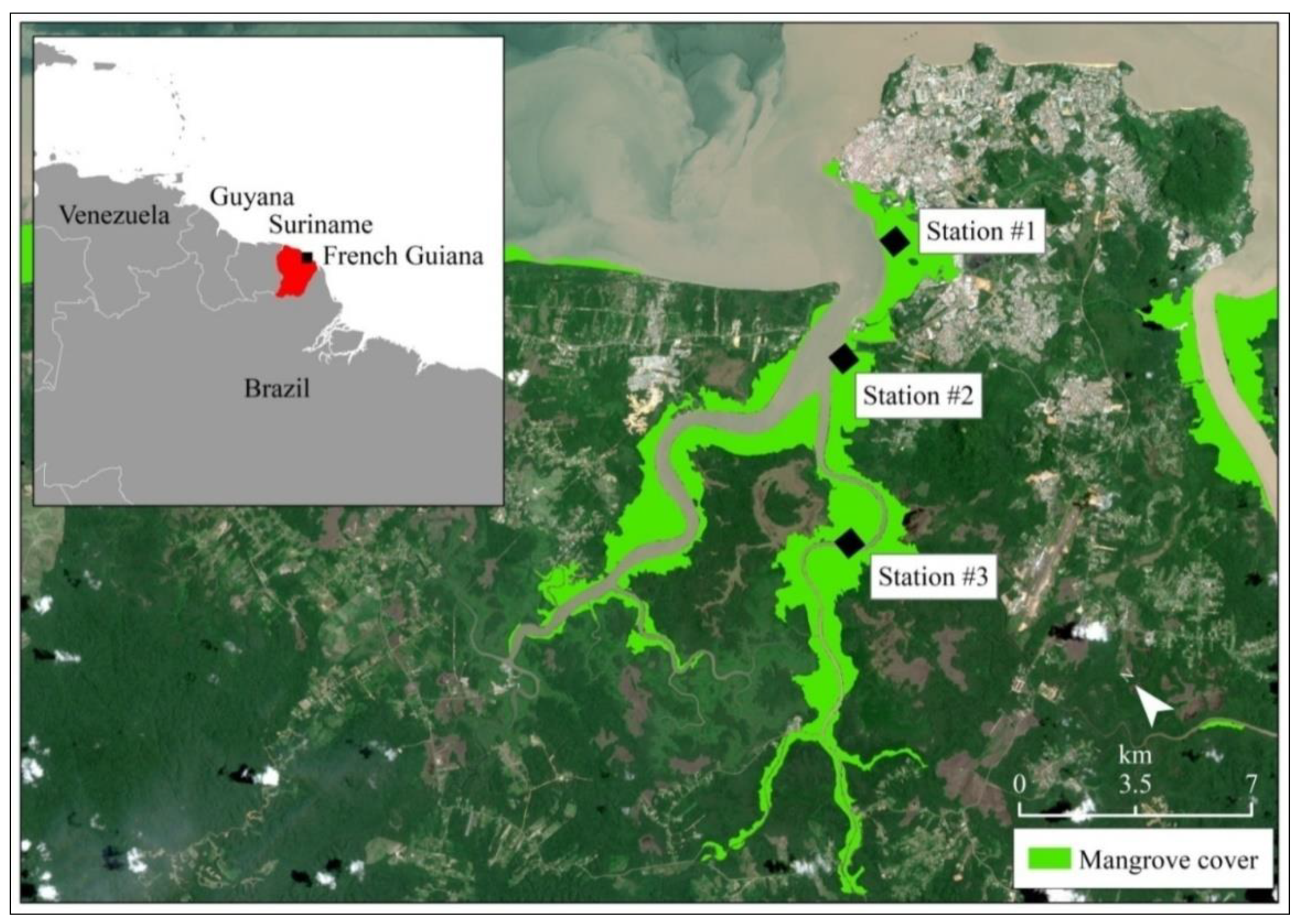
2.1. Study Area

The study area was located in the Cayenne estuary, French Guiana (South America, Figure 1). The climate is subtropical with two major rainfall periods extending from late March to early July and from mid-November to early March. Tides are semidiurnal and mesotidal with a mean tidal range of 1.68 m. FG is part of the French oversea departments and regions and is characterized by a 320 km-long mangrove coast, largely dominated by A. germinans, Rhizophora spp., and Laguncularia racemosa (C.F. Gaertn., 1807). A. germinans constitutes the often monospecific and homogeneous in adult ages stands, which characterize most of Guiana’s coastal mangrove [45]. The three mangrove species spread upstream several kilometers inland, following the riverbanks, to the limit of tidal influence [45], and characterize the estuarine mangroves. In FG, the low slope of the coast enhances large salty areas at the estuary mouths where mangroves grow several kilometers inland. Despite the large amount of Amazonian waters, the FG coast exhibits high salinity [46]. In fact, the freshwater itself remains far from the shore during the dry season, following the north Brazilian current, while only the mud plume arrives at the coast. The three stations investigated in this study were located on the edges of the estuary (<5 m from the river channel) colonized by the adult mangroves, at an increasing distance from the Cayenne city (Figure 1). The three stations exhibited the same mean sediment elevations (1.02 ± 0.08 m) as revealed by the Digital Elevation Model (Figure S1A). They were all characterized by a similar adult mangrove stand-age with the same mean canopy height above the terrestrial reference (Figure S1B), and all of them were dominated by A. germinans and Rhizophora spp., being proxies of constant salinity range over estuary at a similar tidal time [49]. Station 1 was located near a wastewater treatment plant, which drained the waters from industrial, commercial, and urban activity at “Crique Fouillée” coming out of Cayenne city (4°54′53.208′′ N; 52°20′15.9324′′ W, Figure 1) [47,50]. Station 2 was located at the intersection between two rivers, Cayenne and Montsinnery, near to agricultural parcels (4°53′49.2288′′ N; 52°22′27.714′′ W, Figure 1). Station 3 was established 10km from the estuary mouth and from the agricultural and urban environments, located upstream the main “Cayenne” River, along the “Petit Cayenne” River (4°51′31.9716′′ N; 52°23′59.5248′′ W, Figure 1), making it the reference station. These stations were all located within the estuarine polyhaline zone, with the same salinity variations ranges as indicated by previous studies [46]. At the time of our sampling, at the rising tides of the spring tides during the dry season, the stations, all located in the same polyhaline area, presented a similar range of salinity for surface water comprised (p > 0.05) between 30 ± 2 (station 1) and 28 ± 2 (station 2) to 25 ± 3 (station 3).

2.2. Field Sampling

The stations were sampled between 19 and 21 of November 2017, during the spring tides, two hours before the high tide. High tide made the sampling stations easily accessible. However, the sampling sites were not inundated at high tide. Only station 2 presented thin water layer above sediment, which did not prevent the sampling. Three sediment cores (plexiglass tubes of 10.4 cm internal diameter, 20 cm height each) were manually collected from each station, each core being distanced of about 2m. Sediment cores were sliced horizontally from 0 to 2 cm (L1), 2 to 10 cm (L2), and 10 to 16 cm depth (L3), making three main sediments layers (L1, L2, L3) for each sediment core. Redox potential (Eh) and pH were measured directly in the core for each sediment layer using a multi-parameter system coupled to soil specific probes WTW Multi 3500i. Instrument precision was ±0.01 Eh and ±0.001 pH, the latter calibrated with NBS Buffers. Within each sediment layer, six sediment subsamples were extracted for the analysis of grain size, total carbon (TC) and nitrogen (TN), inorganic and organic contaminant concentrations, pigments content, prokaryotic biomass, and meiofauna, respectively. Inox spatulas and pyrolyzed glass bottles (450 °C, 3 h) were used to sample sediments for analysis of organic contaminants. Plastic spoons and 15 mL falcon tubes were used to sample sediments for metal analyses. Subsamples for grain size analysis were kept in the fridge (4 °C), whereas sediments for biogeochemistry analyses were directly frozen (−80 °C). Subsamples with a sub-surface area of 1.77 cm² were taken in each sediment layer for meiofauna analysis. The meiofauna samples were fixed in 4% diluted formaldehyde buffered with sodium bicarbonate and stored cold until analysis.

2.3. Laboratory Analyses

2.3.1. Grain Size, Carbon and Nitrogen Bulk Analyses

Sediments were freeze-dried (24 h) and gently crushed to powder and homogenized for bulk sediment analyses. Sedimentary grain size distribution was determined using a laser beam diffraction analyzer (Partica LA-950V2; Horiba Instruments, Inc.). Total Carbon (TC) and Total Nitrogen (TN) were analyzed by combustion at 930 °C using a CHN carbon analyzer (Flash-2000; Thermo Fisher Scientific Inc., Milan, Italy). Due to the lack of carbonates in the FG region [51], the organic fractions largely dominated or equally corresponded to the total carbon. The total carbon and nitrogen were thus used as proxies of the organic matter, and the molar C:N ratio was calculated to infer a proxy of the refractory versus labile nature of the organic matter.

2.3.2. Pigment Analysis

Lipophilic pigments were analyzed by high-performance liquid chromatography (HPLC) [52]. Mangrove sediments were incubated with 95% methanol (buffered with 2% ammonium acetate) during 15 min, at −20°C in the dark. Extracts were then filtered with 0.2μm PTFE syringe filters and analyzed within 16h using an Agilent 1260 Infinity HPLC composed of a quaternary pump (VL 400 bar), a UV–VIS photodiode array detector (DAD 1260 VL, 190–950nm), a fluorescence detector (FLD 1260 excitation: 425 nm, emission: 655nm), and a 100μL automatic sample injector refrigerated at 4°C in the dark. Chromatographic separation was carried out using a C18 column for reverse phase chromatography (Supelcosil, 25 cm long, 4.6 mm inner diameter). The solvents used were: 0.5M ammonium acetate in methanol and water (85:15, v:v), acetonitrile and water (90:10, v:v), and 100% ethyl acetate. The solvent gradient was set [52], with a 0.5 mL min⁻¹ flow rate. Identification and calibration of the HPLC peaks were performed with antheraxanthin, ββ-carotene, canthaxanthin, chlorophyll a, chlorophyll b, chlorophyll c2, diatoxanthin, diadinoxanthin, fucoxanthin, and pheophytin a standards. We identified all detected peaks by their absorption spectra and relative retention times using the Agilent OpenLab software. Quantification was performed using standard calibration curves built with repeated injections of standards over a range of dilutions. Xanthophylls, carotenes, and chlorophyll b and c were quantified at 470 nm, and chlorophyll a and their derivatives as well as pheopigments were quantified at 665 nm. The relative abundance of each pigment (%) was calculated from its respective concentration in the sample (μg mg⁻¹).

2.3.3. Metals and Metalloids Analysis

Sediments were digested using an aqua regia and microwave assistant. Then, the obtained solutions were filtered through 0.2 µm (cellulose nitrate, Sartorius) and diluted for analysis. Concentrations of minor/major/trace elements were measured by High-Resolution Inductively Coupled Plasma—Mass Spectrometer (HR—ICP/MS, Element 2, Finnigan) and validated by using SLRS-5 (River water certified reference material, National Research Council of Canada—NRC), LGC (River certified reference), and PACS2 (NRC) for sediments. The analytical recovery was within 10% compared to certified concentration. Particulate Hg was analyzed on aliquots of 50 mg dry sediment using a cold vapor atomic absorption spectrometry (CV-AAS; Leco Ama 254) equipped with a low-level optical cell. The method detection limit, estimated as three times standard deviation of the blank samples, was 2 pg. The certified reference material MESS-4 (National Research Council Canada) was run several times per analytical batch and constantly before starting the measurements, to check the accuracy of the measurements. The measured values were always within ±5% of the recommended values.

2.3.4. Organic Contaminants Analysis

Six groups of organic chemicals were analyzed including 16 polycyclic aromatic hydrocarbons (PAHs), 6 polychlorinated biphenyls (PCB), 12 organochloride pesticides, 6 phthalates, 7 polybromodiphenylethers (PBDE), and 2 alkylphenols. Sediment extraction, clean-up, and analysis followed published methods [53]. The main differences corresponds to the purification step, which is conducted with SPE cartridge (Interchim, France; [54]) and to the analytical equipment, a GC-MS/MS is preferred in order to increase the sensitivity. Analytical method is fully described [55]. For PAHs, PCB and pesticides quantification naphthalene D8, biphenyl D10, phenanthrene D10, pyrened10, chrysene D12, benzo(a)pyrene D12, benzo(g,h,i)perylene D12 were used as standards. For the plastic additives (phthalates and PBDE), di (2-ethylhexyl) phthalate D4 and BDE 77 were respectively used as standards. All standards were obtained from LGC Standard (Wesel, Germany) and Interchim (Montluçon, France).

2.3.5. Bacterial and Archaeal Abundance

Total DNA was extracted from composite sediment samples representative of each layer (0.25–0.30 gdry sediment) using the PowerSoil DNA isolation kit (MoBio) according to the manufacturer’s recommendations. The bacterial and archaeal abundance was measured by real-time quantitative PCR (qPCR), by the determination of bacterial and archaeal 16S rRNA gene copy numbers, respectively [56]. The resulting conditions lead to a quantitative PCR efficiency higher than 99% (R² = 0.99). 16S rRNA genes abundances were standardized by the mass of DNA recovered per g dry sediment.

2.3.6. Meiofauna Analysis

Meiofauna organisms were extracted from sediment samples [57]. Particles were conserved in Falcon tube containing a solution of formaldehyde with drops of Rose Bengal. The meiofauna was identified at the highest taxonomic level possible under a binocular lens (Stemi 508 binocular lens) and were measured with a micrometer screw (length and width). 150 nematodes per sample were collected; they were mounted on permanent slides according to the formalin–ethanol–glycerol treatment and identified under an optical microscope [57,58]. Nematodes were classified in groups according to their trophic groups. Four groups were identified based on morphology characters: Absence or fine buccal cavity—bacterivorous; large buccal cavity without teeth—non-selective detritivores; buccal cavity with scraping teeth—grazers; and buccal cavity with large jaws—omnivorous-predators [59,60]. The maturity index (MI) assigned values from 1 for extremely opportunistic nematodes to 5 for extremely sensitive nematodes and according to life-history traits and their adaptability to a new environment [61]. The MI (Bongers, 1990) for a nematode assemblage was calculated as the weighted mean of the individual taxon scores:

$$MI={\displaystyle \sum }_{i=1}^n{v}_i\times f_i$$

where $v_i$was the c-p value of taxon I and $f_i$was the frequency of that taxon.

Meiofauna density and biomass were calculated at all sampling stations and along a vertical profile into the sediment. Density was expressed as number of individuals per 10cm². Biomass calculation was done in µg of carbon per 10cm² [57].

2.4. Statistical Analyses

Multiple factor analyses (MFA), which are extension of principal component analyses (PCA), are devoted to the study of tables in which groups of variables are introduced to the analysis (instead of using all the variables at once; [62]). This method can deal with tables that have many explicative variables and share the same statistical individuals. The variables are weighted so that in case of unbalanced groups of variables, the analysis will not be influenced by the largest group. The weights are identical for the variables of the same group (and vary from one group to another). They are such that the maximum axial inertia of a group is equal to 1. We thus used MFA analyses with the R package “ade4” [63] in order to find the links between several groups (matrix) of variables measured on the same set of statistical individuals (i.e., biological, physical, biogeochemical, and meiofauna variables on the same sediment core, and/or at the same sediment depth). The overall analysis consisted here in introducing several active groups (for instance: Physico-chemical parameters, metals, contaminants, prokaryotic biomass, organic matter, pigments) in a factorial analysis in order to analyze similarities and discrepancies between groups [64]. Two MFAs were carried out, one with environmental factors and the other with the density and biomass of the meiofauna. On the other hand, the studied entities came from the same samples (in the same sample were extracted several data), which allowed us to compare the two MFA between them thereafter.

Separated PCAs were then performed on each group of variables: One with environmental factors, one with the density of nematodes, and one with the biomass of nematodes and then a weight equal to the inverse of the first Eigen value of the PCA was assigned to each group before concatenating them in a single dataset. Additionally, in order to explore the weight of a given factor (e.g., sediment depth or the interaction between sampling station and sediment depth), we performed a supervised Between Class Analysis (BCA) by decomposing the total inertia of the MFA dataset according to a given instrumental variable (i.e., sampling stations, and/or sediment depth). Percentage of total inertia explained by the instrumental variable was systematically calculated ([63]; hereafter called bca-ratio). The above mentioned statistical procedure was previously detailed [65] and was performed (i) on the sediment parameters measured at each sampling stations (i.e., environmental variables: 3 variables (granulometry, pH, redox potential); pigments: 31 variables; prokaryotic biomass: 2 variables (archaeal and bacterial); organic matter quality: 2 variables (C:N ratio and organic carbon content); contaminants: 18 variables (organic and inorganic contaminants); (ii) on the nematodes density and iii) on the nematodes biomass, grouped by their feeding behavior (i.e., bacterivorous, detritivores, grazers, omnivorous predators). A threshold based on the square cosine of the coordinates of the variables was applied for highlighting the most discriminating variables. A Monte Carlo test was systematically performed to test the significance of the BCA ordination.

We have verified the significance of the most discriminating sediment variables, between the stations, by testing the station (station 1, 2, and 3) and depth effects (L1, L2, L3) on them with variances analysis. When the normality (Shapiro–Wilk test) and homogeneity of the variances were met (Bartlett test), Anova (analysis of variance) followed by Tukey (for pairwise comparisons) tests were carried out. Otherwise, non-parametric tests of Sheirer–Ray–Hare (SRH) test with Wilcoxon (for pairwise comparisons) were carried out [66].

Since the meiofauna occurred mainly over the first 5 cm depths, we tested the influence of station on the overall meiofauna diversity variables (density, biomass, trophic, and maturity indexes) by using a non-parametric one-way analysis of variance (Kruskal–Wallis test) following by Wilcoxon (for pairwise comparisons). The same analysis was done to test the station effect on each taxonomic unit of the meiofauna community (Foraminifera, Acarina, Nematoda, Copepoda, Kinorhyncha, Plathyelminths, Ostracoda).

A permutational multivariate analysis of variance, using a Bray–Curtis dissimilarity index (PERMANOVA; [67]), based on density and biomass per matrix of nematode genus group, was computed to test the multivariate response of infauna assemblages to the station location after verifying the multivariate homogeneity of group dispersions. Correlation analyses were then used to quantify the relatedness between nematodes genus and environmental variables, using the non-parametric Spearman coefficient $\rho$ as data normality was not verified. These analyses were done using the software R (version 3.5.1) and Rcommander.

3. Results

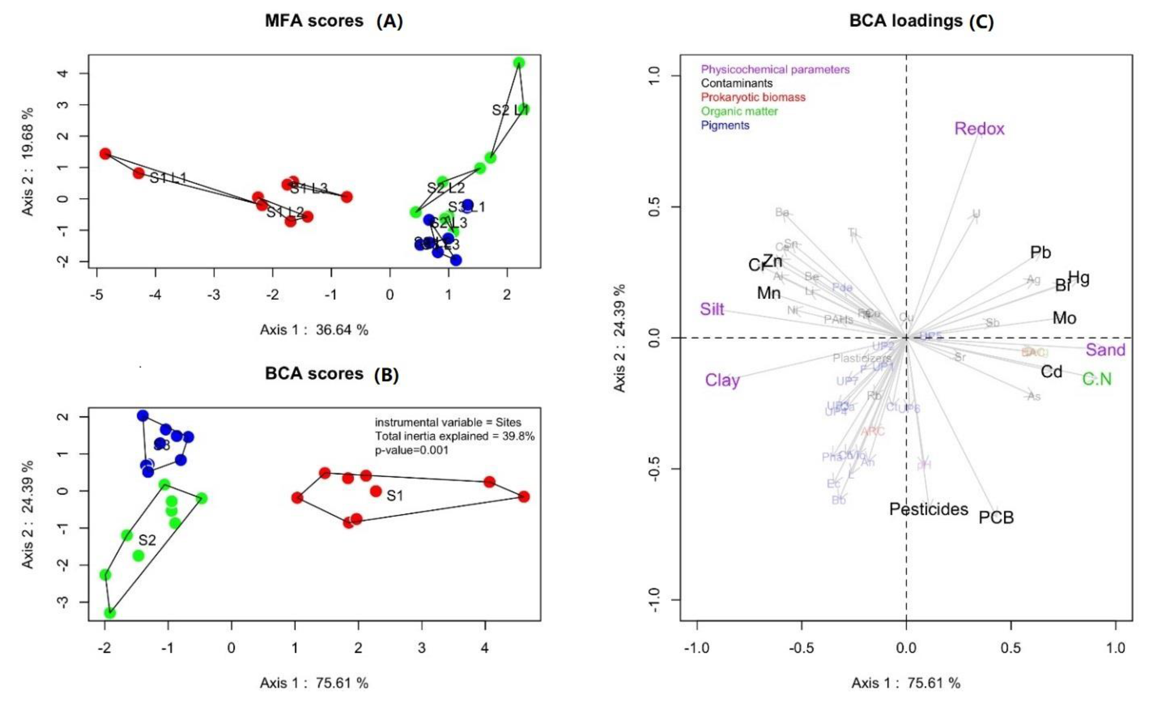
3.1. Environmental Characteristics

The first axis of the Multiple factor analyses (MFA), based on the environmental variables at each depth and station, explained 36.6% and the second axis explained 19.7% of the variance (Figure 2A). MFA analysis showed that the three layers of each station (L1, L2, L3) were grouped together (Figure 2A). Then, the first axis of the supervised Between Class Analysis (BCA) on the same environmental variables dataset explained 75.6% and the second axis explained 24.4% of the variance (Figure 2B). Station 1 was separated from the other stations by the axis 1 and stations 2 and 3 were separated by the axis 2 (Figure 2B). The supervised analysis (BCA; Figure 2C) showed that 39.8% of total inertia (i.e., bca-ratio) was explained by the sampling stations. The first axis was defined by variations in organic contaminants and metals types, prokaryotic biomasses (archaeal versus bacterial), granulometry (silt and clay versus sand), and organic matter (C:N) while physico-chemical parameters (pH and redox potential) and pigments (Pheophorbide a- Pda versus all other pigments) defined the second axis.

Among these physical and biogeochemical sediment variables defining the two axis, we have defined the most discriminant ones with a square cosine of the coordinates superior to 0.4 (Figure 2C; cos² > 0.4) and the most significant ones (Figure S2; p < 0.005). Thus, we have determined that the significant higher proportion of sand and the higher contents of metals (i.e., mercury (Hg), molybdenum (Mo), bismuth (Bi), cadmium (Cd), arsenic (As), and lead (Pb)), number of copies of the bacterial 16S, total organic carbon (TOC), and C:N ratio characterized station 1 (

Table 1. Mean values of the three cores over the entire sedimentary column from each station for the physical, chemical, and biological parameters (mean ± SD; n = 3).

	Station 1	Station 2	Station 3
	Physico-chemical parameters
Ph	6.26 ± 0.03	6.36 ± 0.11	6.02 ± 0.07
Redox potential (mV)	119 ± 8.51	−90.1 ± 24.4	159 ± 5.78
	Granulometry (%)
Clay	3.59 ± 0.40	8.34 ± 0.55	7.23 ± 0.44
Silt	75.3 ± 0.68	87.2 ± 1.33	88.3 ± 0.57
Sand	20.2 ± 0.34	4.20 ± 0.91	4.08 ± 0.93
	Carbon and Nitrogen
Total Organic Carbon (TOC %)	0.04 ± 0.01	0.02 ± 0.002	0.01 ± 0.0005
C:N (mol/mol)	15.5 ± 0.86	10.3 ± 0.70	9.49 ± 0.18
	Prokaryotic community (number of 16S gene copies mg−1d.w.)
ARC 16S	5.50×103 ± 1.87×103	1.18×104 ± 5.46×103	4.37×103 ± 2.56×103
BAC 16S	3.89×106 ± 1.40×106	5.76×105 ± 1.99×104	3.83×105 ± 6.80×104
	Pigments concentrations (µg cm−3)
Antheraxanthin (An)	5.84 ± 1.29	20.7 ± 6.66	2.07 ± 0.52
Beta-caroten (Bb)	0.16 ± 0.06	1.06± 0.25	0.06 ± 0.04
Canthaxanthin (Ct)	0.38 ± 0.27	0.58 ± 0.38	0.29 ± 0.19
Chlorophyll a (Ca)	1.22 ± 0.42	5.20 ± 2.31	2.27 ± 0.71
Chlorophyllb (Cb)	0.14± 0.04	1.37 ± 0.58	0.16 ± 0.03
Echinenone (Ec)	0.21 ± 0.14	2.64 ± 1.76	0.20 ± 0.13
Fucoxanthin (F)	3.20 ± 0.89	11.4 ± 6.87	6.97 ± 4.53
Lutein (L)	1.68 ± 0.24	7.20 ± 1.75	1.03± 0.10
Pheophorbidea (Pda)	3.93± 1.56	6.32± 0.51	8.74± 1.95
Pheophytin a (Pha)	20.8 ± 4.95	47.0 ± 1.36	23.6± 0.86
UnknownPigment 1 (UP1)	1.51 ± 0.94	2.90 ± 2.46	1.83 ± 1.14
Unknown Pigment 2 (UP2)	1.66 ± 1.23	2.71 ± 1.80	2.38 ± 0.82
UnknownPigment 3 (UP3)	0.91 ± 0.24	4.15 ± 0.86	2.01 ± 0.56
UnknownPigment 4 (UP4)	0.15 ± 0.20	1.21 ± 0.23	0.48 ± 0.34
UnknownPigment 5 (UP5)	1.13 ± 0.26	0.89 ± 0.29	0.92 ± 0.34
UnknownPigment 6 (UP6)	0.38 ± 0.21	0.45 ± 0.17	0.26 ± 0.15
UnknownPigment 7 (UP7)	0.23 ± 0.07	0.44 ± 0.01	0.33 ± 0.06
Violaxanthin (Vio)	1.65 ± 0.97	4.06 ± 1.08	1.41 ± 0.23
	Concentrations of organic contaminants (ng g−1)
Hydrocarbons	48.6 ± 17.6	212 ± 20.3	250 ± 79.0
Pesticides	11.9 ± 1.81	10.8 ± 0.87	0.03 ± 0.04
PCB	3.43 ± 0.31	4.95 ± 2.48	0.21 ± 0.28
Plasticizers	0.00	0.45 ± 0.60	0.28 ± 0.21
	Concentrations of metals ad metalloids (µg g−1)
Aluminum (Al)(mg g−1)	110 ± 1.86	115 ± 1.78	118 ± 1.37
Antimony (Sb)	0.64 ± 0.07	0.54 ± 0.02	0.56 ± 0.002
Arsenic (As)	25.9 ± 1.28	22.7 ± 1.25	21.3 ± 0.31
Barium (Ba)	400 ± 6.27	416 ± 6.76	440 ± 4.79
Beryllium (Be)	3.13 ± 0.10	3.24 ± 0.07	3.32 ± 0.04
Bismuth (Bi)	0.59 ± 0.01	0.53 ± 0.01	0.55 ± 0.01
Cadmium (Cd)	0.08 ± 0.01	0.07 ± 0.005	0.07 ± 0.002
Cesium (Cs)	11.5 ± 0.08	11.9 ± 0.24	12.4 ± 0.14
Chromium (Cr)	78.6 ± 2.75	84.5 ± 1.50	87.5 ± 0.73
Cobalt (Co)	20.7 ± 2.14	21.3 ± 1.32	21.8 ± 0.18
Copper (Cu)	29.6 ± 1.79	29.4 ± 0.65	29.8 ± 0.47
Iron (Fe) (mg g-1)	63.0 ± 3.31	64.2 ± 4.71	65.0 ± 2.85
Lead (Pb)	36.8 ± 1.11	32.6 ± 0.60	34.7 ± 0.23
Lithium (Li)	83.4 ±2.23	86.3 ± 1.43	87.8 ± 1.12
Manganese (Mn)	420 ± 41.3	862 ± 182	992 ± 87.4
Mercury (Hg) (ng g-1)	59.7 ± 2.70	47.0 ± 0.05	51.0 ± 1.11
Molybdenum (Mo)	2.12 ± 0.09	1.31 ± 0.09	1.43 ± 0.01
Nickel (Ni)	36.7 ± 1.31	38.5 ± 0.72	38.8 ± 0.35
Rubidium (Rb)	129 ± 1.47	200 ± 93.7	132 ± 1.36
Silver (Ag)	0.23 ± 0.01	0.16 ± 0.02	0.19 ± 0.01
Strontium (Sr)	122 ± 14.6	116 ± 0.99	114 ± 1.09
Thallium (Tl)	0.92 ± 0.02	0.92 ± 0.02	0.97 ± 0.01
Tin (Sn)	3.58 ± 0.07	3.70 ± 0.08	3.83 ± 0.04
Titanium (Ti)(mg g-1)	2.70 ± 0.44	2.80 ± 0.26	2.86 ± 0.13
Uranium (U)	2.25 ± 0.10	1.78 ± 0.21	2.23 ± 0.02
Vanadium (V)	153 ± 5.9	161 ± 3.50	167 ± 1.49
Zinc (Zn)	136 ± 9.07	148 ± 3.01	156 ± 1.48

, Figure 2C, Figure S2). Station 2 was distinguished by higher proportion of clay, negative redox potential (Eh), and pigments increase, i.e., Violaxanthin (Vio), Beta-carotene (Bb), Antheraxanthin (An), Lutein (L) (Table 1, Figure 2C, Figure S2). The significant higher proportions in PCB and pesticides also qualified stations 1 and 2 (Table 1, Figure 2C, Figure S2). Finally, significant higher concentrations of PAHs and specific metals, i.e., Zn, Ba (Table 1, Figure 2C, Figure S2) mostly differentiated station 3. We found the highest proportions of silt and higher quantities of Vanadium (V), Chromium (Cr), and Manganese (Mn) in stations 2 and 3.

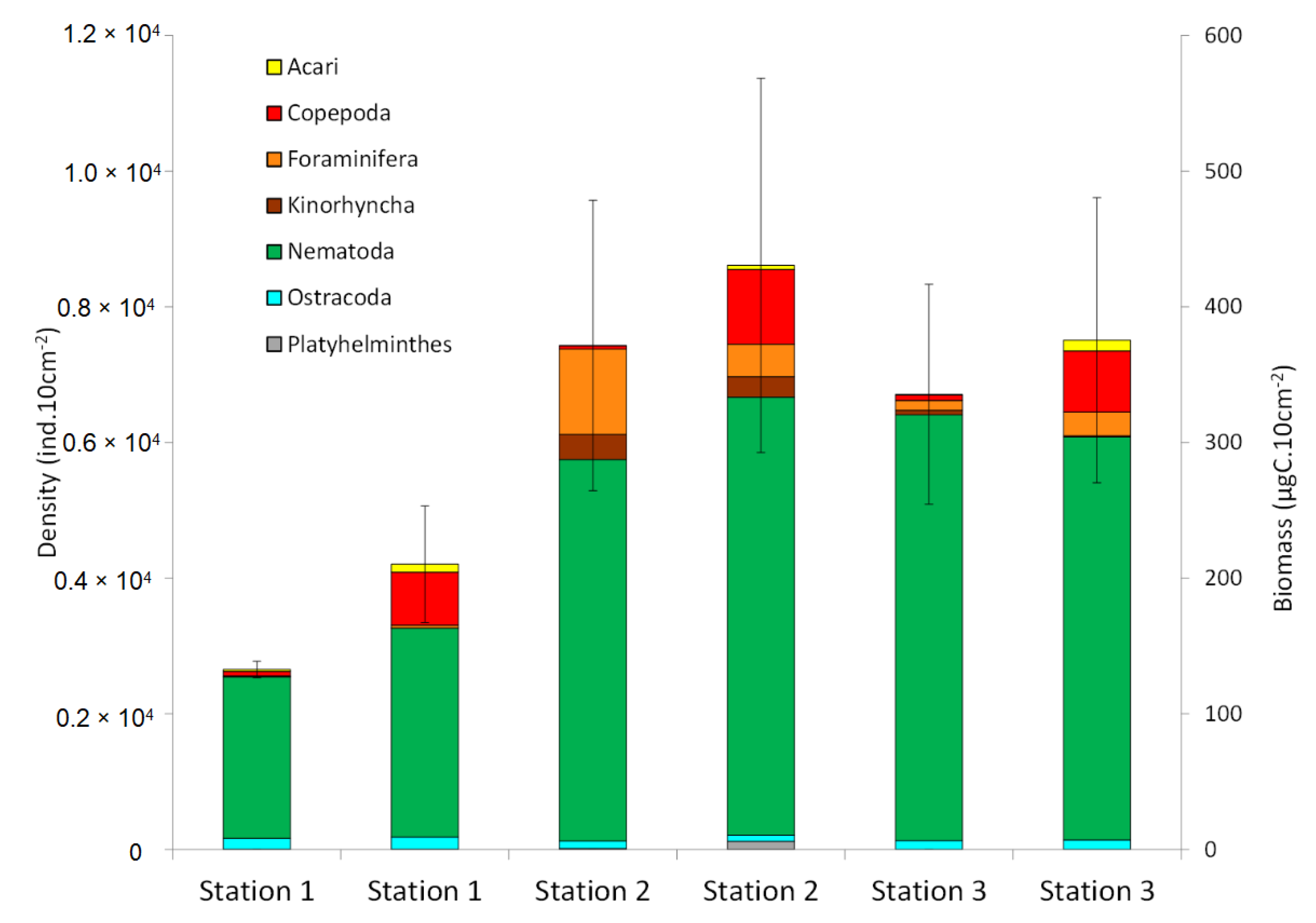
3.2. Total Meiofauna Community

Total densities of the overall benthic meiofauna community varied from 2651 ± 121 individuals per 10 cm² at station 1, to 7431 ± 2141 individuals per 10 cm² at station 2 and 6712 ± 1619 individuals per 10cm² at station 3 (Figure 3), but they were not significantly different. However, densities of certain taxa were different among stations. Foraminifera were found in higher abundances at station 2 (Kruskal–Wallis test; p = 0.03) whereas Acarina showed higher density values at station 1 (Kruskal–Wallis tests; p = 0.03). Nematoda was the most abundant taxon at all sampling stations: 76% at station 2, 90% at station 1, and 93.5% at station 3 (Figure 3).

Total meiofaunal biomass ranged from 210 ± 43 µgC per 10 cm² at station 1, 404 ± 138 µgC per 10 cm² at station 2, and 375 ± 105 µgC per 10 cm² at station 3 (Figure 3), but they were not significantly different.

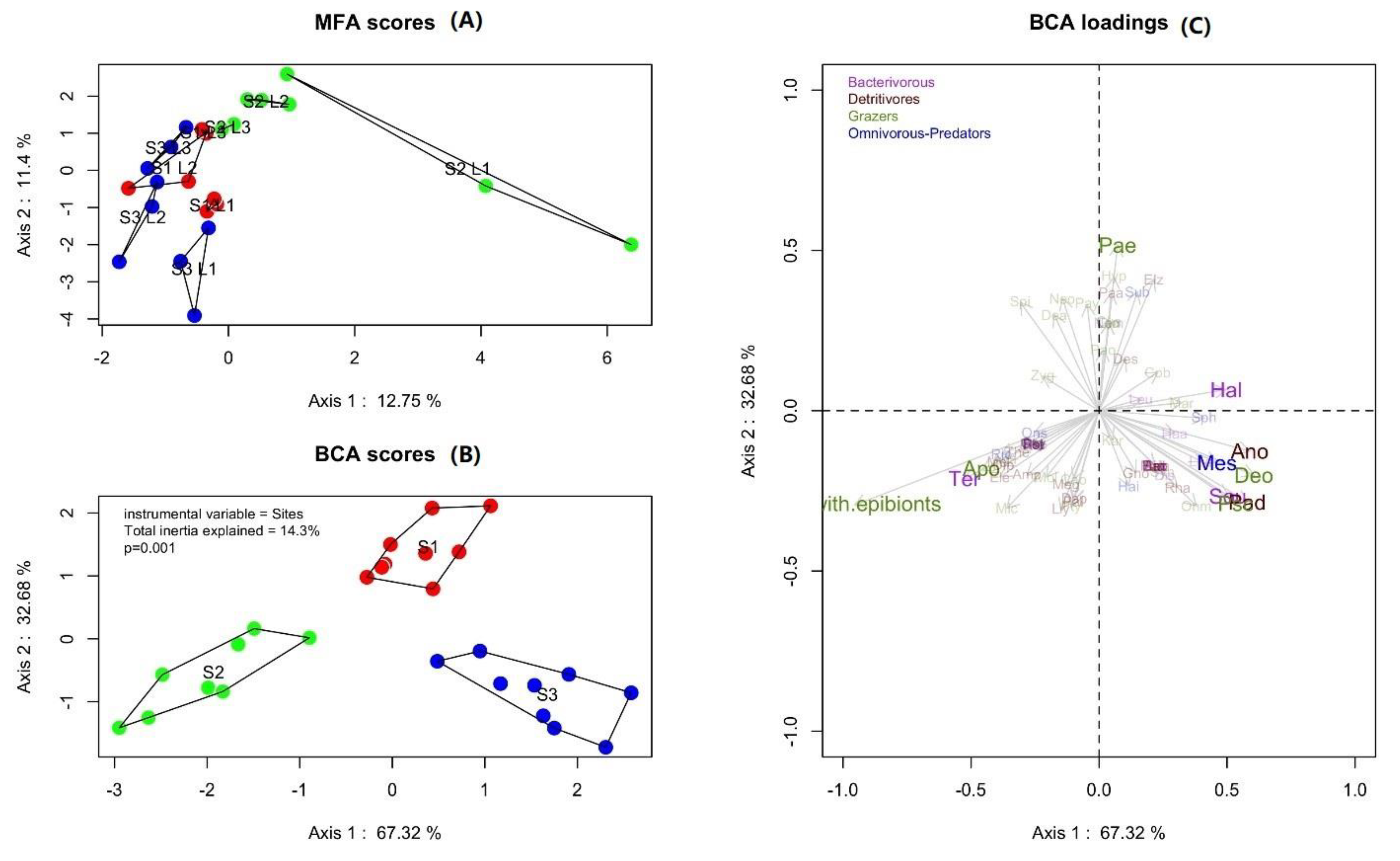
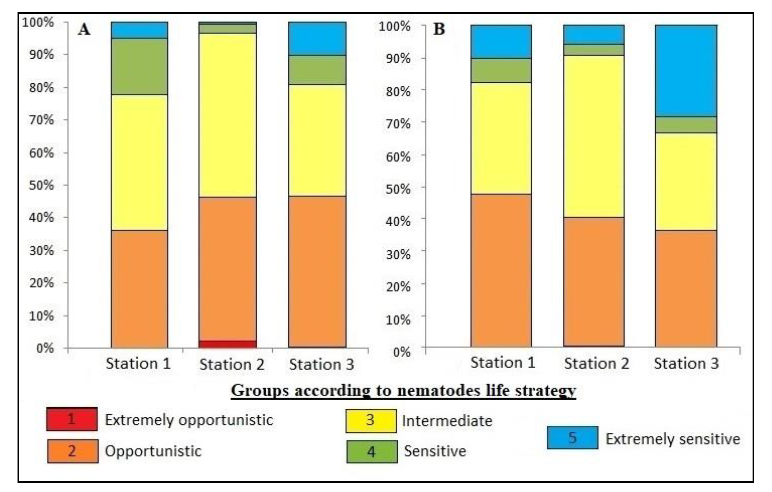
3.3. Nematoda Community

Nematodes genera richness did not differ significantly between stations. Nematodes were significantly more abundant in the surface layers (0–2 cm; p < 0.05) at stations 1 and 2 (>80%) and at station 3 (>60%).

The two first axes of the unsupervised analysis (MFA) explained 24% of the total variance (Figure 4A). The MFA analysis showed a differentiation of the three stations based on L1 whereas L2 and L3 are grouped. The supervised BCA analysis showed that 14% of total inertia was explained by the sampling stations and showed a differentiation of the three stations based on the nematodes genera relative abundance: Station 1 along the axis 1 and stations 2 and 3 along the axis 2 (Figure 4B,C). The cos² threshold of 0.2 highlighted the most structuring genus of nematodes (Figure 4C). The PERMANOVA analysis (not shown here) allows us to affirm that nematodes composition is different between stations (p < 0.001).

Seventy-three nematode genera were observed (all stations combined) and 18 were present at all three stations, including the Desmodora, Terschellingia, Paracomesoma (Schuurmans Stekhoven, 1950), and Microlaimus (de Man, 1880) (Figure S3).

Thirty-seven nematode genera were identified at station 1, and the Desmodora and Spirinia genera accounted for more than 35% of the total nematode abundance at this station. However, the genus Paraethmolaimus significantly discriminated the station 1 (

Table 2. Mean total nematode densities (individuals per 10cm²; ±SD) and mean relative nematode densities (%; ±SD) at each station (here reported nematodes with at least 2% density on one station). The nematoda exhaustive list including those with a relative density < 2% is presented in Figure S3 with their appartenance trophic groups.

Family	Genus	AbbreViation	Station 1		Station 2		Station 3
			Density ind.10cm−2	Relative Density (%)	Density ind.10cm−2	Relative Density (%)	Density ind.10cm−2	Relative Density (%)
Anoplostomatidae	Anoplostoma	Ano	113 ± 71	5 ± 3	0	0	452 ± 128	7 ± 0.5
Axonolaimidae	Parodontophora	Pad	28 ± 19	12 ± 8	0	0	294 ± 43	5 ± 1
Camacolaimidae	Deontolaimus	Deo	99 ± 55	4 ± 2	0	0	508 ± 79	9± 3
Chromadoridae	Hypodontolaimus	Hyp	130± 63	6 ± 3	0	0	0	0
	Neochromadora	Neo	56 ± 27	2 ± 1	73 ± 69	1 ± 1	8 ± 10	0.2 ± 0.2
	Ptycholaimellus	Pty	0	0	214 ± 121	3 ± 2	100± 52	2 ± 1
Desmodoridae	Desmodora	Dea	648 ± 158	27 ± 6	912 ± 517	14.5 ± 7	293 ± 132	6 ± 3
	Spirinia	Spi	252 ± 154	10 ± 6	343 ± 92	7 ± 4	0	0
Diplopeltidae	Southerniella	Sou	7 ± 9	0.3 ± 0.4	0	0	163 ± 94	2 ± 1
Ethmolaimidae	Paraethmolaimus	Pae	114 ± 118	5 ± 5	0	0	0	0
Leptosomatidae	Pseudocella	Psc	77 ± 21	3 ± 1	39 ± 52	1 ± 1	670± 275	10 ± 3
Linhomoeidae	Metalinhomoeus	Mel	0	0	193 ± 107	3 ± 2	0	0
	Paralinhomoeus	Pal	5 ± 6	0.2 ± 0.2	164 ± 109	2.5 ± 2	61 ± 58	1 ± 1
	Terschellingia	Ter	96 ± 47	4 ± 2	1410± 525	28 ± 12	14.5 ± 19	3 ± 4
Microlaimidae	Microlaimus	Mic	15 ± 8	1 ± 0.4	367 ± 248	8 ± 7	1178 ± 560	17 ± 6.5
	Molgolaimus	Mol	5 ± 6	0.2 ± 0.3	140 ± 102	2 ± 2	39 ± 17	1 ± 0.1
Oxystominidae	Halalaimus	Hal	185 ± 41	8 ± 2	144 ± 96	2 ± 1.5	583 ± 273	9 ± 2
Selachinematidae	Richtersia	Ric	5 ± 6	0.2 ± 0.3	245 ± 198	4 ± 3	0	0
Sphaerolaimidae	Metasphaerolaimus	Mes	320± 220	1 ± 1	0	0	151 ± 70	2.5 ± 1
	Sphaerolaimus	Sph	64 ± 40	3 ± 2	39 ± 52	1 ± 1	222 ± 84	3.5 ± 1
	Subsphaerolaimus	Sub	48 ± 17	2 ± 1	0	0	7± 6	1 ± 1
Xyalidae	Daptonema	Dap	0	0	183 ± 122	3 ± 2	84 ± 62	1 ± 1
	Cobbia	Cob	36 ± 10	1.5 ± 0.5	65 ± 33	1 ± 1	19 ± 8	3 ± 1
	Elzalia	Elz	109 ± 34	5 ± 2	43 ± 50	1 ± 1	263 ± 105	4 ± 1
	Zygonemella	Zyg	8 ± 4	3 ± 1.5	287 ± 191	4 ± 3	35 ± 23	1 ± 0.4

, Figure 4C).

At station 2, we identified 45 nematode genera and Terschellingia genus alone accounted for 27% of the nematode abundance at this station. The presence of Terschellingia significantly distinguished station 2 from the two other stations (Figure 4C, Table 2).

In addition, we observed the presence of epibionts on nematodes of the genus Desmodora at stations 1 (i.e., 2.2%) and 2 (i.e., 23.5%).

Station 3 hosted 50 nematodes genera. Genera Pseudocella, Anoplostoma (Bütschli, 1874), Deontolaimus (de Man, 1880), Parodontophora (Timm, 1963), and Halalaimus (de Man, 1888) were the most represented at station 3 (Figure 4C, Table 2).

Spirinia genus was significantly less present at station 3, as well as the Halalaimus genus at station 2, whereas Ptycholaimellus (Cobb, 1920) genus was less observed at station 1 (Table 2). The same analysis based on the relative biomass of nematodes was carried out and show roughly the same results (Figure S4).

Correlation coefficients (Figure S5) were calculated between the significant environmental variables discriminating the stations and the nematodes genera. In station 1, the genus Paraethmolaimus was positively correlated with sand ($\rho =0.56$), C:N ratio ($\rho =0.61$) and high concentrations of metals, Pb ($\rho =0.40$), Mo ($\rho =0.45$) and Hg ($\rho =0.52$). In station 2, genera Terschellingia and Desmodora with epibionts were positively correlated with the presence of PCB-type organic contaminants ($\rho =0.70$), but only nematodes-epibionts showed negative correlations with redox potential ($\rho =-0.76$). At station 3, we observed a negative correlation between genera Pseudocella and Deontolaimus with the presence of organic contaminants (PCB and Pesticides) ($\rho =-0.60$) and positive correlations between genera Halalaimus, Anoplostoma, Deontolaimus, Pseudocella, and redox potential ($\rho ~ 0.40 to 0.60$).

Regarding the trophic groups of nematodes based on the nematodes densities, grazers were the most represented in all the stations with a higher grazing density at station 1 and predators the least ones (p < 0.05; Figure 5; Figure S3). The trophic diversity index, based on the nematode trophic groups, was higher at station 1 (0.48 ± 0.05) than at stations 2 and 3 (0.36 ± 0.03) (p < 0.03). However, we observed no difference in the proportion of the different trophic groups of nematodes based on the nematodes biomass.

The nematodes maturity was based on their adaptability to a new environment, which makes it possible to classify nematodes in very opportunistic (and therefore very adaptable) genera up to very sensitive (and not very adaptable) genera. The nematode maturity index did not differ between stations (2.5 ± 0.05 to 2.9 ± 0.02). However, we noticed that opportunistic and intermediate nematodes were the most abundant at each station (Figure 5A) (p < 0.05). Station 2 had the highest value of opportunistic nematodes of all stations, in terms of abundance (p < 0.02).

Relative to the total nematode densities within each station, we observed that stations 1 and 2 were made up of a higher proportion of opportunistic and intermediate nematodes (p < 0.05; Figure 5B).

The differentiation of station 3 took place at the level of the biomass of extremely opportunistic nematodes, which was the lowest (p < 0.02; Figure 5B).

Regarding the differentiation of stations at the level of nematode biomasses per maturity groups, only the biomass values of extremely opportunistic nematodes varied from one station to another. Station 2 showed more extremely opportunistic individuals (p < 0.02; Figure 5B).

4. Discussion

4.1. Environmental Characteristics of the Three Stations

The overall studied stations, although located within similar mangrove stand age and along the polyhaline estuarine area, have shown distinct and significant different sediment variables. Although the dominant mode of grain size remained the silt for each station over all the sedimentary column, we think, however, station 1 was likely more impacted by the proximity to the seafront since the sand mode was more important at this station. Both stations 1 and 3 were dominated by aerobic redox conditions (Eh~100–200 mV) while the sediments of station 2 showed negative dominant anaerobic patterns with negative redox potential (Eh~−100mV), an indicator of the less oxidized sediments. We have found a dominance of the mangroves litter pigments (i.e., Antheraxanthin, Lutein, Beta-carotene, and Violaxanthin) at station 2, thus highlighting an organic enrichment. On the contrary, although C:N ratio of 16–20 indicated more refractory material at station 1, the 16S DNA increase was the sign of numerous bacterial cells and suggested a higher bacterial OM degradation and mineralization at this station. However, archaeal abundances were about 10 (stations 2 and 3) to 1000-fold (station 1) lower than those of bacteria (Table 1), but they were not considered as a discriminant variable (low cos² < 0.4) in the multiple factor analysis (MFA) and between class analysis (BCA), and our interpretation on the prokaryotic community remained based on the bacterial abundances.

We have noticed a strong presence of pesticides and PCB at stations 1 and 2 that were relatively absent from station 3. Such organic contaminants, likely anthropogenic, might come from the wastewater treatment plant (“Crique Fouillée”) located near station 1, and from agricultural parcels and by river runoff having a greater impact on station 2 [47,50]. Among the organic chemical components, we have also measured 4 to 5-fold higher concentrations of PAHs at stations 2 and 3 than station 1. By drawing a comparison with polluted mangrove areas where PAHs concentrations levels are up to several thousand ng/g [68], we have concluded that PAHs concentrations measured in the Cayenne estuary remained low. We think most of the PAHs found in coastal sediments of French Guiana are probably from pyrolytic origin (wood burning [69], maintenance of coastal savannas [21]) due to a low industrialization and a still-low human population density. In our case, we think that PAHs can more easily accumulate in finer sediments (station 2 and 3) but also when sediment organic content is higher (station 1) [70]. Here, differences were most probably due to differences in the number of atmospheric inputs and, perhaps, to a somehow easier accumulation in the sediments.

By referring to the official guideline concentrations for assessing toxicity hazards (i.e., effects range low (ERL) and effects range median (ERM; NOAA, 2012)), we have seen that organic contaminants and metals concentrations remained low. The most toxic PCB in our analyses were dioxin-like polychlorinated biphenyl 169 with a total concentration of 19.1 µg.kg⁻¹ being just below the official used threshold [71] which does however depend on various intrinsic sediments parameters as the OM content. The most abundant pesticide was hexachlorobenzen found at station 2 at a concentration below the level of 17 ng/g that is calculated to be a predicted no effect HCB concentration for chronic exposure (PNEC_chronic) for organisms living in sediments [72]. We think that the different natural physical and biogeochemical context between the stations explained the high variations of metal concentrations. As example, we know that metals origin might be lithogenic with a succession of co-precipitation and co-complexification geochemical processes as already observed in another Guianese mangroves area [73]. However, the metals Pb, Hg, Mo, and Bi clearly characterized the station 1 likely due to the proximity to a wastewater treatment plant (“Crique Fouillée”). In this station, Pb (39.95 mg/kg) and Hg (0.64 mg/kg) concentrations were just above the thresholds from which metals can potentially affect benthic invertebrates but below lethal thresholds [74,75,76].

Station 3, located downstream of the Cayenne estuary still in the polyhaline area, received less contaminants and its more oxidized sediments revealed reactive biogeochemical functioning. At a similar tidal level to the station 1, metals as well as organic contaminants were less present at station 3 due to its distance from the Cayenne city, urban wastewater, and agricultural impacts. We thus think, as expected, this reference station is more preserved than the other two stations from anthropogenic effects.

Interestingly, we found the presence of a degradation pigment (Pheophorbide a-Pda) at station 3 and pheophytins a at station 2. The first step of chlorophyll a degradation in plants is hydrolysis of the phytyl ester bond by chlorophyllase to form chlorophylide a and phytol. In the second step, chlorophylide a is demetallized to form Pheophorbide a [77]. Pheophorbide a is thus a degradation product of chlorophylide a while pheophytin a is a degradation product of chlorophyll a. The presence of these two pigments could indicate different degradation processes between the two stations (stations 2 and 3) either in terms of metabolism or in terms of source of organic matter for invertebrates. Chlorophyll degradation could be advantageous in plants by preventing the accumulation of excited free chlorophyll or if protein amino acids must be redeployed for alternative needs in case of nutritional deficiency [78].

4.2. Overall Meiofauna Community

Meiofauna is generally more resistant than macrofauna and increases in density in the presence of organic and industrial contaminants [79]. However, this is true until a threshold level, after that a decrease in density is usually observed [80]. A previous study [81] had highlighted that mangrove meiofauna abundance is higher in undisturbed sediments compared to sediments disturbed by anthropogenic activities (e.g., from 2.6 ± 1.1 to 1.6 ± 4.41 individuals per 10cm²).

In our study, meiofauna diversity did not vary significantly between stations. Nevertheless, its community structure was significantly different among the stations. Higher Foraminifera density at station 2 confirmed the presence of less oxygenated sediment [82,83,84]. In low oxygen concentrations, Foraminifera set up specific mechanisms, in particular decreasing their size [85,86]. In the present study, Kinorhyncha reached almost 5% (station 2) of the overall meiofauna, which is in the range of values reported from stressful environments (e.g., wide fluctuations of salinities [87,88,89], while they are usually less than <5% in shallow waters and deep-sea ecosystems [30].

4.3. Nematodes Community

The deeper identification we made on the nematodes genera has brought more detailed indications of sediment conditions, as also confirmed by other experimental works [33]. Previous studies shown that salinity differences among the four haline zones of an entire estuary (i.e., euhaline, polyhaline, mesohaline, oligohaline; [90]) can control the distribution of the nematoda assemblages [91]. In our case, we excluded the salinity effect since the three stations were all located within the same polyhaline zone of the estuary. We sampled during the dry season, but during the wet season the estuary salinity decrease [92] might impact the nematoda assemblages over a year for the same stations, as observed in some Vietnamese estuaries [93]. In a study based on the metals impacts (e.g., Hg, Pb, As, Cd, Cu, and Cr) on meiofauna assemblages [40], authors supported the evidence of some nematode tolerance against metals loads whose concentrations exceeded the National Environment Quality. However, in our study, lower trace metal concentrations, supposed to be mainly of lithogenic origin, might affect nematodes community. At station 1, the genus Paraethmolaimus was dominant and significantly correlated to the presence of Hg, Pb, Cd, and Mo. In fact, recent work has underscored nematodes strong sensibility to low metals concentrations [94].

In our study, the genus Terschellingia accounted for 27% of the nematodes at station 2 (Table 2) where it was correlated with the presence of PCB contaminants, but also a site with the highest densities and biomass of opportunistic nematoda. The dominance of a nematode genus is typical during a disturbance, with tolerant genera taking over sensitive organisms. The genus Terschellingia is known to be highly tolerant to organic contaminants [95], and particularly to PCB [96], and accounts for more than 10% of the nematode community in disturbed stations [97,98]. In addition to being dominant in organic-rich sediments [99], this genus is known to be adapted to the low oxidized muddy environments [100], which was the case for station 2 as indicated by the highly negative redox potential. Although high abundance of Terschellingia can be used as an indicator of polluted environments [101], other studies showed that this genus was unable to adapt to high metal concentrations [39] which might be the case in station 2 where metals concentrations remained low. Even if Terschellingia spp. tolerates organic enrichment, their activity levels and functions in benthic habitats can decline under oxygen limitation [102]. This case illustrates how the species in this Genus, characterized by different life cycles, respond to a wide range of organic contamination/enrichment regimes.

At station 3, the five abundant genera (Southerniella Allgén, 1932; Pseudocella, Deontolaimus, Halalaimus, and Anoplostoma) accounted for more than 50% of the total nematode abundance. The genera Pseudocella and Halalaimus are not tolerant to environmental disturbances and variations [61]. In our study, the genus Pseudocella accounted for 10% of nematode abundance. Thus, its presence indicated an absence or weak environmental disturbance at station 3. In addition, we noticed a low presence of the genus Spirinia, which demonstrated its stress tolerance, physiological, and behavioral adaptability to environmental disturbances in previous studies [36,99,103]. As the sediments of stations 3 were well oxidized without organic-rich material neither contaminants, we concluded that station 3 presented stable environmental conditions for those sensitive and highly sensitive nematodes.

The Desmodora genus was present at the three stations in similar proportions. This genus is known to adapt to different environmental conditions [95,99]. Its presence in the three stations can be explained by its adaptability. However, we observed Desmodora with epibionts only at stations 1 and 2 (Figure 6). These epibionts, classified as suctorian ciliates [104], were found almost exclusively on the genus Desmodora: station 1 has lower epibionts values (2.2%) than station 2 (23.5%). A co-occurrence between epibionts and organic contaminants may support the fact that this epibiosis could be the result of a decrease in the immunity of organisms induced by stress, such as disrupted environmental conditions. Ciliate epibiosis is a common phenomenon in marine nematodes. As recently reported [104], the presence of epibionts on nematodes cuticle (which is involved in vital functions such as exchange of gases and nutrients, info-chemicals, and defense metabolites) can have a high cost for the host. Two to three epibionts already cause stress for the basibiont whereas more than five epibionts increase the energetic demand for locomotion [105]. Furthermore, it has been shown that in a variety of marine ecosystems, the presence of epibionts on nematodes was reported only in the most stressful condition sites (both due to anthropogenic actions or naturally extreme conditions) [104]. The occurrence of epibionts in a mangrove ecosystem could be due to habitat heterogeneity and the nature of anthropogenic disturbance [106]. Environmental stressful conditions can promote epibiosis because nematodes are more vulnerable and easily infested ([104]; and references therein) promoting the use of epibiosis as ecological indicator in the assessment of ecological mangrove status.

We classified the majority of nematodes as epistrate feeders, as previously reported [107]. The high grazers abundance in our study has indicated the presence of algae and vegetal debris accessible to nematodes. This is typically the case of mangroves where organisms have direct access to mangroves leaves and products of their degradation. We also observed that most of the representative nematodes were grazers [107], at the stations with a higher organic-rich sediment, highlighted by the dominance of mangroves litter pigments and of the degradation pigments. Station 2 was dominated by selective deposit feeders (e.g., Terschellingia) and epistrate feeders (e.g., Desmodora, Spirinia, Microlaimus). The presence of selective and non-selective deposit feeder nematodes indicated the presence of organic detritus that could result from the release of wastewater into the environment [108]. Opportunistic and Intermediate nematodes were the most abundant at all sampling stations. These life strategies are common between nematodes genera that are able to colonize impacted and unstable environments but also undisturbed ones. Our data can be partially explained by the high natural environmental variability typical of mangroves. A previous study [109] also showed similar maturity index values in both disturbed and preserved environments. However, the fact that station 3 hosted higher abundances and biomass of very sensitive nematodes confirmed that impacts in this station were lower allowing the surviving of sensitive organisms.

5. Conclusions

We showed that the use of nematodes can provide accurate information to characterize the quality of the mangroves environment rather the investigation of the overall meiofauna community. An accurate identification of Foraminifera and Kinorhyncha in FG also should help in the future. This study confirmed that the structure of nematodes community varied according to the sediments characteristics. The presence of organic chemical components (PAHs, pesticides, PCB) and metals, even at low concentrations, in addition to redox state of the sediments, might influence meiofauna composition. The different concentrations of metals found at the three stations, which were below ERM and for most of the metals close to ERL, still resulted in a response from meiofauna and nematodes. Our results show that Paraethmolaimus, Terschellingia, Spirinia, and Desmodora and associated epibionts might be the first indicators of a pollution onset, while the sensible genus Pseudocella could be an indicator of absence or very low contamination rate. This information needs to be acquired in areas where human impacts are absent or low and before environmental threats are present. These data sets and information can inform the preparation of pollution management programs in case where the input of sediments with high organic and metal concentrations are occurring or expected. However, further studies of mangrove meiofauna at different spatial and temporal scales (e.g., seasons) from a large range of geographical locations with different levels of deterioration are essential for strengthening our conclusions on the use of Nematoda as bioindicator taxon of mangroves ecological status. Because the response of Nematoda can differ according to the type of disturbance, future work dedicated to mangrove management programs or restoration strategies should also include speciation analysis of metals (e.g., methylmercury, As (III/V)) and organic chemical components (e.g., pesticides, PCB) within mangroves sediments and surrounding waters.

References

1. Valiela, I.; Bowen, J.L.; York, J.K. Mangrove Forests: One of the World’s Threatened Major Tropical Environments. BioScience 2001, 51, 807–815. [Google Scholar] [CrossRef] [Green Version]
2. Worthington, T.; Spalding, M. Mangrove Restoration Potential: A Global Map Highlighting a Critical Opportunity; University of Cambridge: Cambridge, UK, 2018; pp. 1–34. [Google Scholar] [CrossRef]
3. Worthington, T.A.; zu Ermgassen, P.S.E.; Friess, D.A.; Krauss, K.W.; Lovelock, C.E.; Thorley, J.; Tingey, R.; Woodroffe, C.D.; Bunting, P.; Cormier, N.; et al. A Global Biophysical Typology of Mangroves and Its Relevance for Ecosystem Structure and Deforestation. Sci. Rep. 2020, 10, 14652. [Google Scholar] [CrossRef]
4. Adeel, Z.; Pomeroy, R. Assessment and Management of Mangrove Ecosystems in Developing Countries. Trees 2002, 16, 235–238. [Google Scholar] [CrossRef]
5. Goldberg, L.; Lagomasino, D.; Thomas, N.; Fatoyinbo, T. Global Declines in Human-Driven Mangrove Loss. Glob. Change Biol. 2020, 26, 5844–5855. [Google Scholar] [CrossRef] [PubMed]
6. Field, C.B.; Osborn, J.G.; Hoffman, L.L.; Polsenberg, J.F.; Ackerly, D.D.; Berry, J.A.; Bjorkman, O.; Held, A.; Matson, P.A.; Mooney, H.A. Mangrove Biodiversity and Ecosystem Function. Glob. Ecol. Biogeogr. Lett. 1998, 7, 3–14. [Google Scholar] [CrossRef]
7. Lee, S.Y.; Primavera, J.H.; Dahdouh-Guebas, F.; McKee, K.; Bosire, J.O.; Cannicci, S.; Diele, K.; Fromard, F.; Koedam, N.; Marchand, C.; et al. Ecological Role and Services of Tropical Mangrove Ecosystems: A Reassessment. Glob. Ecol. Biogeogr. 2014, 23, 726–743. [Google Scholar] [CrossRef]
8. Hai, N.T.; Dell, B.; Phuong, V.T.; Harper, R.J. Towards a More Robust Approach for the Restoration of Mangroves in Vietnam. Ann. For. Sci. 2020, 77, 18. [Google Scholar] [CrossRef] [Green Version]
9. Kodikara, K.A.S.; Mukherjee, N.; Jayatissa, L.P.; Dahdouh-Guebas, F.; Koedam, N. Have Mangrove Restoration Projects Worked? An in-Depth Study in Sri Lanka. Restor. Ecol. 2017, 25, 705–716. [Google Scholar] [CrossRef]
10. Richards, D.R.; Thompson, B.S.; Wijedasa, L. Quantifying Net Loss of Global Mangrove Carbon Stocks from 20 Years of Land Cover Change. Nat. Commun. 2020, 11, 4260. [Google Scholar] [CrossRef]
11. Alongi, D.M. Impact of Global Change on Nutrient Dynamics in Mangrove Forests. Forests 2018, 9, 596. [Google Scholar] [CrossRef] [Green Version]
12. McKee, K.L.; Cahoon, D.R.; Feller, I.C. Caribbean Mangroves Adjust to Rising Sea Level through Biotic Controls on Change in Soil Elevation. Glob. Ecol. Biogeogr. 2007, 16, 545–556. [Google Scholar] [CrossRef]
13. Bosire, J.O.; Dahdouh-Guebas, F.; Walton, M.; Crona, B.I.; Lewis, R.R.; Field, C.; Kairo, J.G.; Koedam, N. Functionality of Restored Mangroves: A Review. Aquat. Bot. 2008, 89, 251–259. [Google Scholar] [CrossRef] [Green Version]
14. Thornton, S.R.; Johnstone, R.W. Mangrove Rehabilitation in High Erosion Areas: Assessment Using Bioindicators. Estuar. Coast. Shelf Sci. 2015, 165, 176–184. [Google Scholar] [CrossRef]
15. Allard, S.M.; Costa, M.T.; Bulseco, A.N.; Helfer, V.; Wilkins, L.G.E.; Hassenrück, C.; Zengler, K.; Zimmer, M.; Erazo, N.; Rodrigues, J.L.M.; et al. Introducing the Mangrove Microbiome Initiative: Identifying Microbial Research Priorities and Approaches To Better Understand, Protect, and Rehabilitate Mangrove Ecosystems. mSystems 2020, 5. [Google Scholar] [CrossRef] [PubMed]
16. Romañach, S.S.; DeAngelis, D.L.; Koh, H.L.; Li, Y.; Teh, S.Y.; Raja Barizan, R.S.; Zhai, L. Conservation and Restoration of Mangroves: Global Status, Perspectives, and Prognosis. Ocean Coast. Manag. 2018, 154, 72–82. [Google Scholar] [CrossRef]
17. Cuny, P.; Jezequel, R.; Michaud, E.; Sylvi, L.; Gilbert, F.; Fiard, M.; Chevalier, C.; Morel, V.; Militon, C. Oil Spill Response in Mangroves: Why a Specific Ecosystem-Based Management Is Required? The Case of French Guiana – a Mini-Review. Vie et Milieu 2020, in press. [Google Scholar]
18. Dirberg, G.; Barnaud, G.; Brivois, O.; Caessteker, P.; Corlier-Salem, M.; Cuny, P.; Fromard, F.; Fiard, M.; Gilbert, F.; Grouard, S.; et al. Towards the Development of Ecosystem-Based Indicators of Mangroves Functionin State in the Context of the EU Water Framework Directive. Vie et Milieu 2020, in press. [Google Scholar]
19. Dauvin, J.-C.; Bellan, G.; Bellan-Santini, D. Benthic Indicators: From Subjectivity to Objectivity – Where Is the Line? Mar. Pollut. Bull. 2010, 60, 947–953. [Google Scholar] [CrossRef] [PubMed]
20. Sandulli, R.; De Nicola-Giudici, M. Pollution Effects on the Structure of Meiofaunal Communities in the Bay of Naples. Mar. Pollut. Bull. 1990, 21, 144–153. [Google Scholar] [CrossRef]
21. Zeppilli, D.; Sarrazin, J.; Leduc, D.; Arbizu, P.M.; Fontaneto, D.; Fontanier, C.; Gooday, A.J.; Kristensen, R.M.; Ivanenko, V.N.; Sørensen, M.V.; et al. Is the Meiofauna a Good Indicator for Climate Change and Anthropogenic Impacts? Mar. Biodivers. 2015, 45, 505–535. [Google Scholar] [CrossRef] [Green Version]
22. Alongi, D. Inter-Estuary Variation and Intertidal Zonation of Free-Living Nematode Communities in Tropical Mangrove Systems. Mar. Ecol. Prog. Ser. 1987, 40, 103–114. [Google Scholar] [CrossRef]
23. Netto, S.A.; Gallucci, F. Meiofauna and Macrofauna Communities in a Mangrove from the Island of Santa Catarina, South Brazil. Hydrobiologia 2003, 505, 159–170. [Google Scholar] [CrossRef]
24. Pinto, T.K.; Austen, M.C.V.; Warwick, R.M.; Somerfield, P.J.; Esteves, A.M.; Castro, F.J.V.; Fonseca-Genevois, V.G.; Santos, P.J.P. Nematode Diversity in Different Microhabitats in a Mangrove Region. Mar. Ecol. 2013, 34, 257–268. [Google Scholar] [CrossRef]
25. Aschenbroich, A.; Michaud, E.; Gilbert, F.; Fromard, F.; Alt, A.; Le Garrec, V.; Bihannic, I.; De Coninck, A.; Thouzeau, G. Bioturbation Functional Roles Associated with Mangrove Development in French Guiana, South America. Hydrobiologia 2017, 794, 179–202. [Google Scholar] [CrossRef] [Green Version]
26. Riera, P.; Hubas, C. Trophic Ecology of Nematodes from Various Microhabitats of the Roscoff Aber Bay (France): Importance of Stranded Macroalgae Evidenced through Δ13C and Δ15N. Mar. Ecol. Prog. Ser. 2003, 260, 151–159. [Google Scholar] [CrossRef] [Green Version]
27. Schratzberger, M.; Ingels, J. Meiofauna Matters: The Roles of Meiofauna in Benthic Ecosystems. J. Exp. Mar. Biol. Ecol. 2018, 502, 12–25. [Google Scholar] [CrossRef]
28. Mutua, A.K.; Ntiba, M.J.; Muthumbi, A.; Ngondi, D.; Vanreusel, A. Restoration of Benthic Macro-Endofauna after Reforestation of Rhizophora Mucronata Mangroves in Gazi Bay, Kenya. West. Indian Ocean J Mar Sci 2011, 10, 39–49. [Google Scholar]
29. Balsamo, M.; Semprucci, F.; Frontalini, F.; Coccioni, R. Meiofauna as a Tool for Marine Ecosystem Biomonitoring. Mar. Ecosyst. 2012. [Google Scholar] [CrossRef] [Green Version]
30. Della Patrona, L.; Marchand, C.; Hubas, C.; Molnar, N.; Deborde, J.; Meziane, T. Meiofauna Distribution in a Mangrove Forest Exposed to Shrimp Farm Effluents (New Caledonia). Mar. Environ. Res. 2016, 119, 100–113. [Google Scholar] [CrossRef] [PubMed] [Green Version]
31. Bowman, A.W. An Alternative Method of Cross-Validation for the Smoothing of Density Estimates. Biometrika 1984, 71, 353–360. [Google Scholar] [CrossRef]
32. Gee, J.M.; Warwick, R.M.; Schaanning, M.; Berge, J.A.; Ambrose, W.G. Effects of Organic Enrichment on Meiofaunal Abundance and Community Structure in Sublittoral Soft Sediments. J. Exp. Mar. Biol. Ecol. 1985, 91, 247–262. [Google Scholar] [CrossRef]
33. Haegerbaeumer, A.; Höss, S.; Ristau, K.; Claus, E.; Heininger, P.; Traunspurger, W. The Use of Meiofauna in Freshwater Sediment Assessments: Structural and Functional Responses of Meiobenthic Communities to Metal and Organics Contamination. Ecol. Indic. 2017, 78, 512–525. [Google Scholar] [CrossRef]
34. Zeppilli, D.; Leduc, D.; Fontanier, C.; Fontaneto, D.; Fuchs, S.; Gooday, A.J.; Goineau, A.; Ingels, J.; Ivanenko, V.N.; Kristensen, R.M.; et al. Characteristics of Meiofauna in Extreme Marine Ecosystems: A Review. Mar. Biodivers. 2018, 48, 35–71. [Google Scholar] [CrossRef] [Green Version]
35. Brustolin, M.C.; Nagelkerken, I.; Fonseca, G. Large-Scale Distribution Patterns of Mangrove Nematodes: A Global Meta-Analysis. Ecol. Evol. 2018, 8, 4734–4742. [Google Scholar] [CrossRef] [PubMed]
36. Warwick, R.M.; Price, R. Ecological and Metabolic Studies on Free-Living Nematodes from an Estuarine Mud-Flat. Estuar. Coast. Mar. Sci. 1979, 9, 257–271. [Google Scholar] [CrossRef]
37. Sahoo, G.; Suchiang, S.R.; Ansari, Z.A. Meiofauna-Mangrove Interaction: A Pilot Study from a Tropical Mangrove Habitat. Cah. Biol. Mar. 2013, 54, 349–358. [Google Scholar]
38. Gyedu-Ababio, T.K.; Baird, D. Response of Meiofauna and Nematode Communities to Increased Levels of Contaminants in a Laboratory Microcosm Experiment. Ecotoxicol. Environ. Saf. 2006, 63, 443–450. [Google Scholar] [CrossRef]
39. Austen, M.C.; Somerfield, P.J. A Community Level Sediment Bioassay Applied to an Estuarine Heavy Metal Gradient. Mar. Environ. Res. 1997, 43, 315–328. [Google Scholar] [CrossRef]
40. Nasira, K.; Shahina, F.; Kamran, M. Response of Free-Living Marine Nematode Community to Heavy Metal Contaminantion along the Coastal Areas of Sindh and Balochistan Pakistan. Pak. J. Nematol. 2010, 28, 263–278. [Google Scholar]
41. Monteiro, L.; Brinke, M.; dos Santos, G.; Traunspurger, W.; Moens, T. Effects of Heavy Metals on Free-Living Nematodes: A Multifaceted Approach Using Growth, Reproduction and Behavioural Assays. Eur. J. Soil Biol. 2014, 62, 1–7. [Google Scholar] [CrossRef]
42. Bunting, P.; Rosenqvist, A.; Lucas, R.M.; Rebelo, L.M.; Hilarides, L.; Thomas, N.; Hardy, A.; Itoh, T.; Shimada, M.; Finlayson, C.M. The Global Mangrove Watch - A New 2010 Global Baseline of Mangrove Extent. Remote Sens. 2018, 10, 1669. [Google Scholar] [CrossRef] [Green Version]
43. Anthony, E.J.; Gardel, A.; Gratiot, N.; Proisy, C.; Allison, M.A.; Dolique, F.; Fromard, F. The Amazon-Influenced Muddy Coast of South America: A Review of Mud-Bank–Shoreline Interactions. Earth-Sci. Rev. 2010, 103, 99–121. [Google Scholar] [CrossRef]
44. Proisy, C.; Couteron, P.; Fromard, F. Predicting and Mapping Mangrove Biomass from Canopy Grain Analysis Using Fourier-Based Textural Ordination of IKONOS Images. Remote Sens. Environ. 2007, 109, 379–392. [Google Scholar] [CrossRef]
45. Lescure, J.-P.; Tostain, O. Les mangroves guyanaises. Bois et Forêts. 1988, 220, 35–42. [Google Scholar]
46. Lambs, L.; Muller, E.; Fromard, F. The Guianese Paradox: How Can the Freshwater Outflow from the Amazon Increase the Salinity of the Guianan Shore? J. Hydrol. 2007, 342, 88–96. [Google Scholar] [CrossRef] [Green Version]
47. Comte, J.; Moungin, B.; Renault, O. Inventaire Des Points de Rejet Sur La Zone Littorale; Report; BRGM: Cayenne, Guyane Française, 2000; p. 46, R 40917 SGR/GUY. [Google Scholar]
48. Recensement de la population en Guyane, 1er Janvier 2018. INSEE. 2020. Available online: https://www.insee.fr/fr/statistiques/5005684 (accessed on 25 January 2021).
49. Fromard, F.; Vega, C.; Proisy, C. Half a Century of Dynamic Coastal Change Affecting Mangrove Shorelines of French Guiana. A Case Study Based on Remote Sensing Data Analyses and Field Surveys. Mar. Geol. 2004, 208, 265–280. [Google Scholar] [CrossRef]
50. Chaneac, L.; Legrand, C. Synthèse Bibliographique Sur Les Zones Humides de Guyane; Rapport Final; BRGM: Cayenne, Guyane Francaise, 2009; p. 137, BRGM/RP-57709-FR. [Google Scholar]
51. Marchand, C.; Lallier-Vergès, E.; Baltzer, F. The Composition of Sedimentary Organic Matter in Relation to the Dynamic Features of a Mangrove-Fringed Coast in French Guiana. Estuar. Coast. Shelf Sci. 2003, 56, 119–130. [Google Scholar] [CrossRef] [Green Version]
52. Brotas, V.; Plante-Cuny, M.-R. The Use of HPLC Pigment Analysis to Study Microphytobenthos Communities. Acta Oecologica 2003, 24, S109–S115. [Google Scholar] [CrossRef]
53. Munschy, C.; Tronczynski, J.; Heas-Moisan, K.; Guiot, N.; Truquet, I. Analyse de contaminants organiques (PCB, OCP, HAP) dans les organismes marins; Méthodes d’analyse en milieu marin; Ifremer/Ministère de l’écologie et du développement durable; Editions Quae: Versailles, France, 2005; ISBN 978-2-84433-144-1. [Google Scholar]
54. Alzaga, R.; Montuori, P.; Ortiz, L.; Bayona, J.M.; Albaigés, J. Fast Solid-Phase Extraction–Gas Chromatography–Mass Spectrometry Procedure for Oil Fingerprinting: Application to the Prestige Oil Spill. J. Chromatogr. A 2004, 1025, 133–138. [Google Scholar] [CrossRef] [PubMed]
55. Lacroix, C.; Le Cuff, N.; Receveur, J.; Moraga, D.; Auffret, M.; Guyomarch, J. Development of an Innovative and “Green” Stir Bar Sorptive Extraction–Thermal Desorption–Gas Chromatography–Tandem Mass Spectrometry Method for Quantification of Polycyclic Aromatic Hydrocarbons in Marine Biota. J. Chromatogr. A 2014, 1349, 1–10. [Google Scholar] [CrossRef] [PubMed]
56. Jézéquel, R.; Duboscq, K.; Sylvi, L.; Michaud, E.; Ferriz, L.M.; Roic, E.; Duran, R.; Cravo-laureau, C.; Michotey, V.; Bonin, P.; et al. Assessment of Oil Weathering and Impact in Mangrove Ecosystem: PRISME Experiment. Int. Oil Spill Conf. Proc. 2017, 634–656. [Google Scholar] [CrossRef]
57. Danovaro, R. Methods for the Study of Deep-Sea Sediments, Their Functioning and Biodiversity; CRC Press: Boca Raton, FL, USA, 2009; ISBN 978-0-429-13096-0. [Google Scholar]
58. Warwick, R.; Platt, H.; Somerfield, P. Free-Living Marine Nematodes: Pictorial Key to World Genera and Notes for the Identification of British Species. Part 3: Monchysterids; Linnean Society of London and the Estuarine and Coastal Sciences Association: Shrewsbury, UK, 1998; p. 296. [Google Scholar]
59. Wieser, W. Free-living marine nematodes. III. Axonolaimoidea and Monhysteroidea. Acta Universitatis Lund 1956, 52, 1–115. [Google Scholar]
60. Moens, T.; Vincx, M. Observations on the Feeding Ecology of Estuarine Nematodes. J. Mar. Biol. Assoc. UK 1997, 77, 211–227. [Google Scholar] [CrossRef]
61. Bongers, T. The Maturity Index: An Ecological Measure of Environmental Disturbance Based on Nematode Species Composition. Oecologia 1990, 83, 14–19. [Google Scholar] [CrossRef] [PubMed]
62. Escofier, B.; Pagès, J. Multiple Factor Analysis (AFMULT Package). Comput. Stat. Data Anal. 1994, 18, 121–140. [Google Scholar] [CrossRef]
63. Dray, S.; Dufour, A.-B. The Ade4 Package: Implementing the Duality Diagram for Ecologists. J. Stat. Softw. 2007, 22, 1–20. [Google Scholar] [CrossRef] [Green Version]
64. Abdi, H.; Williams, L.J.; Valentin, D. Multiple Factor Analysis: Principal Component Analysis for Multitable and Multiblock Data Sets. WIREs Comput. Stat. 2013, 5, 149–179. [Google Scholar] [CrossRef]
65. Lavergne, C.; Hugoni, M.; Hubas, C.; Debroas, D.; Dupuy, C.; Agogué, H. Diel Rhythm Does Not Shape the Vertical Distribution of Bacterial and Archaeal 16S RRNA Transcript Diversity in Intertidal Sediments: A Mesocosm Study. Microb. Ecol. 2018, 75, 364–374. [Google Scholar] [CrossRef]
66. Sokal, R.R.; Rohlf, F.J. Biometry: The Principles and Practice of Statistics in Biological Research, 3rd ed.; W. H. Freeman and Co: New York, NY, USA, 1995. [Google Scholar]
67. Anderson, M.J. Permutational Multivariate Analysis of Variance (PERMANOVA). In Wiley StatsRef: Statistics Reference Online; Wiley Online Library‏: Hoboken, NJ, USA, 2017; pp. 1–15. [Google Scholar] [CrossRef]
68. Tam, N.F.Y.; Ke, L.; Wang, X.H.; Wong, Y.S. Contamination of Polycyclic Aromatic Hydrocarbons in Surface Sediments of Mangrove Swamps. Environ. Pollut. 2001, 114, 255–263. [Google Scholar] [CrossRef]
69. Remy, C.C.; Fleury, M.; Beauchêne, J.; Rivier, M.; Goli, T. Analysis of PAH Residues and Amounts of Phenols in Fish Smoked with Woods Traditionally Used in French Guiana. J. Ethnobiol. 2016, 36, 312–325. [Google Scholar] [CrossRef]
70. Evans, K.M.; Gill, R.A.; Robotham, P.W.J. The PAH and Organic Content of Sediment Particle Size Fractions. Water. Air. Soil Pollut. 1990, 51, 13–31. [Google Scholar] [CrossRef]
71. Arblaster, J.; Ikonomou, M.G.; Gobas, F.A. Toward Ecosystem-Based Sediment Quality Guidelines for Polychlorinated Biphenyls (PCBs). Integr. Environ. Assess. Manag. 2015, 11, 689–700. [Google Scholar] [CrossRef] [PubMed]
72. Pouch, A.; Zaborska, A.; Pazdro, K. The History of Hexachlorobenzene Accumulation in Svalbard Fjords. Environ. Monit. Assess. 2018, 190, 360. [Google Scholar] [CrossRef] [Green Version]
73. Marchand, C.; Lallier-Vergès, E.; Baltzer, F.; Albéric, P.; Cossa, D.; Baillif, P. Heavy Metals Distribution in Mangrove Sediments along the Mobile Coastline of French Guiana. Mar. Chem. 2006, 98, 1–17. [Google Scholar] [CrossRef] [Green Version]
74. MacDonald, D.D.; Ingersoll, C.G.; Berger, T.A. Development and Evaluation of Consensus-Based Sediment Quality Guidelines for Freshwater Ecosystems. Arch. Environ. Contam. Toxicol. 2000, 39, 20–31. [Google Scholar] [CrossRef] [PubMed]
75. Burton, G., Jr. Allen Sediment Quality Criteria in Use around the World. Limnology 2002, 3, 65–76. [Google Scholar] [CrossRef]
76. Conder, J.M.; Fuchsman, P.C.; Grover, M.M.; Magar, V.S.; Henning, M.H. Critical Review of Mercury Sediment Quality Values for the Protection of Benthic Invertebrates. Environ. Toxicol. Chem. 2015, 34, 6–21. [Google Scholar] [CrossRef] [Green Version]
77. Roy, S.; Llewellyn, C.A.; Egeland, E.S.; Johnsen, G. Phytoplankton Pigments: Characterization, Chemotaxonomy and Applications in Oceanography; Cambridge Environmental Chemistry Series; Cambridge University Press: Cambridge, UK, 2011; ISBN 978-1-107-00066-7. [Google Scholar]
78. Hörtensteiner, S. Chlorophyll Degradation During Senescence. Annu. Rev. Plant Biol. 2006, 57, 55–77. [Google Scholar] [CrossRef]
79. Fox, J.F. Intermediate-Disturbance Hypothesis. Science 1979, 204, 1344–1345. [Google Scholar] [CrossRef] [Green Version]
80. Colen, C.V.; Montserrat, F.; Verbist, K.; Vincx, M.; Steyaert, M.; Vanaverbeke, J.; Herman, P.M.J.; Degraer, S.; Ysebaert, T. Tidal Flat Nematode Responses to Hypoxia and Subsequent Macrofauna-Mediated Alterations of Sediment Properties. Mar. Ecol. Prog. Ser. 2009, 381, 189–197. [Google Scholar] [CrossRef] [Green Version]
81. Carugati, L.; Gatto, B.; Rastelli, E.; Lo Martire, M.; Coral, C.; Greco, S.; Danovaro, R. Impact of Mangrove Forests Degradation on Biodiversity and Ecosystem Functioning. Sci. Rep. 2018, 8, 13298. [Google Scholar] [CrossRef] [Green Version]
82. Alve, E. Benthic Foraminiferal Responses to Estuarine Pollution; a Review. J. Foraminifer. Res. 1995, 25, 190–203. [Google Scholar] [CrossRef]
83. Mojtahid, M.; Jorissen, F.; Pearson, T.H. Comparison of Benthic Foraminiferal and Macrofaunal Responses to Organic Pollution in the Firth of Clyde (Scotland). Mar. Pollut. Bull. 2008, 56, 42–76. [Google Scholar] [CrossRef] [PubMed] [Green Version]
84. Luan, B.T.; Debenay, J.-P. Foraminifera, Environmental Bioindicators in the Highly ImpactedEnvironments of the Mekong Delta. Hydrobiologia 2005, 548, 75–83. [Google Scholar] [CrossRef]
85. Bernhard, J.M.; Sen Gupta, B.K. Foraminifera of oxygen-depleted environments. In Modern Foraminifera; Sen Gupta, B.K., Ed.; Springer: Dordrecht, The Netherlands, 2003; ISBN 978-0-306-48104-8. [Google Scholar]
86. Levin, L.A. Oxygen Minimum Zone Benthos: Adaptation and Community Response to Hypoxia. Oceanogr. Mar. Biol. Annu. Rev. 2003, 41, 46. [Google Scholar]
87. Ostmann, A.; Nordhaus, I.; Sørensen, M.V. First Recording of Kinorhynchs from Java, with the Description of a New Brackish Water Species from a Mangrove-Fringed Lagoon. Mar. Biodivers. 2012, 42, 79–91. [Google Scholar] [CrossRef]
88. Yamasaki, H.; Kajihara, H. A New Brackish-Water Species of Echinoderes (Kinorhyncha: Cyclorhagida) from the Seto Inland Sea, Japan. Species Divers. 2012, 17, 109–118. [Google Scholar] [CrossRef] [Green Version]
89. Sørensen, M.V. First Account of Echinoderid Kinorhynchs from Brazil, with the Description of Three New Species. Mar. Biodivers. 2014, 44, 251–274. [Google Scholar] [CrossRef]
90. Montagna, P.A.; Palmer, T.A.; Beseres Pollack, J. Summary: Water Supply, People, and the Future. In Hydrological Changes and Estuarine Dynamics; Montagna, P.A., Palmer, T.A., Beseres Pollack, J., Eds.; SpringerBriefs in Environmental Science; Springer: New York, NY, USA, 2013; pp. 79–81. ISBN 978-1-4614-5833-3. [Google Scholar]
91. Alves, A.S.; Adão, H.; Ferrero, T.J.; Marques, J.C.; Costa, M.J.; Patrício, J. Benthic Meiofauna as Indicator of Ecological Changes in Estuarine Ecosystems: The Use of Nematodes in Ecological Quality Assessment. Ecol. Indic. 2013, 24, 462–475. [Google Scholar] [CrossRef]
92. Ray, R.; Michaud, E.; Aller, R.C.; Vantrepotte, V.; Gleixner, G.; Walcker, R.; Devesa, J.; Le Goff, M.; Morvan, S.; Thouzeau, G. The Sources and Distribution of Carbon (DOC, POC, DIC) in a Mangrove Dominated Estuary (French Guiana, South America). Biogeochemistry 2018, 138, 297–321. [Google Scholar] [CrossRef]
93. Ngo, Q.X.; Nguyen, N.C.; Nguyen, D.T.; Pham, V.L.; Vanreusel, A. Distribution Pattern of Free Living Nematode Communities in the Eight Mekong Estuaries by Seasonal Factor. J. Vietnam. Environ. 2013, 4, 28–33. [Google Scholar] [CrossRef]
94. Haegerbaeumer, A.; Höss, S.; Heininger, P.; Traunspurger, W. Response of Nematode Communities to Metals and PAHs in Freshwater Microcosms. Ecotoxicol. Environ. Saf. 2018, 148, 244–253. [Google Scholar] [CrossRef] [PubMed]
95. Mahmoudi, E.; Beyrem, H.; Aissa, P. Les Peuplements de Nématodes Libres, Indicateurs Du Degré d’anthropisation de La Lagune de Bou Ghrara (Tunisie). Vie et Milieu 2003, 53, 47–59. [Google Scholar]
96. Sahraeian, N.; Sahafi, H.H.; Mosallanejad, H.; Ingels, J.; Semprucci, F. Temporal and Spatial Variability of Free-Living Nematodes in a Beach System Characterized by Domestic and Industrial Impacts (Bandar Abbas, Persian Gulf, Iran). Ecol. Indic. 2020, 118, 106697. [Google Scholar] [CrossRef]
97. Semprucci, F.; Losi, V.; Moreno, M. A Review of Italian Research on Free-Living Marine Nematodes and the Future Perspectives on Their Use as Ecological Indicators (EcoInds). Mediterr. Mar. Sci. 2015, 16, 352–365. [Google Scholar] [CrossRef] [Green Version]
98. Boufahja, F.; Semprucci, F.; Beyrem, H. An Experimental Protocol to Select Nematode Species from an Entire Community Using Progressive Sedimentary Enrichment. Ecol. Indic. 2016, 60, 292–309. [Google Scholar] [CrossRef]
99. Armenteros, M.; Pérez-García, J.A.; Ruiz-Abierno, A.; Díaz-Asencio, L.; Helguera, Y.; Vincx, M.; Decraemer, W. Effects of Organic Enrichment on Nematode Assemblages in a Microcosm Experiment. Mar. Environ. Res. 2010, 70, 374–382. [Google Scholar] [CrossRef] [Green Version]
100. Schratzberger, M.; Warwick, R. Differential Effects of Various Types of Disturbances on the Structure of Nematode Assemblages:An Experimental Approach. Mar. Ecol. Prog. Ser. 1999, 181, 227–236. [Google Scholar] [CrossRef]
101. Soko, M.I.; Gyedu-Ababio, T.K. Free-Living Nematodes as Pollution Indicator in Incomati River Estuary, Mozambique. Open J. Ecol. 2019, 9, 117–133. [Google Scholar] [CrossRef] [Green Version]
102. Steyaert, M.; Moodley, L.; Nadong, T.; Moens, T.; Soetaert, K.; Vincx, M. Responses of Intertidal Nematodes to Short-Term Anoxic Events. J. Exp. Mar. Biol. Ecol. 2007, 345, 175–184. [Google Scholar] [CrossRef]
103. Warwick, R.M.; Gee, J.M. Community Structure of Estuarine Meiobenthos. Mar. Ecol. Prog. Ser. 1984, 18, 97–111. [Google Scholar] [CrossRef]
104. Baldrighi, E.; Dovgal, I.; Zeppilli, D.; Abibulaeva, A.; Michelet, C.; Michaud, E.; Franzo, A.; Grassi, E.; Cesaroni, L.; Guidi, L.; et al. The Cost for Biodiversity: Records of Ciliate–Nematode Epibiosis with the Description of Three New Suctorian Species. Diversity 2020, 12, 224. [Google Scholar] [CrossRef]
105. Fernandez-Leborans, G.; Chatterjee, T.; Grego, M. New Records of Epibiont Ciliates (Ciliophora) on Harpacticoida (Copepoda, Crustacea) from the Bay of Piran (Gulf of Trieste, Northern Adriatic). Cah Biol Mar 2012, 53, 53–63. [Google Scholar]
106. Ansari, K.G.M.T.; Bhadury, P. Occurrence of Epibionts Associated with Meiofaunal Basibionts from the World’s Largest Mangrove Ecosystem, the Sundarbans. Mar. Biodivers. 2017, 47, 539–548. [Google Scholar] [CrossRef]
107. Demopoulos, A.W.J.; Fry, B.; Smith, C.R. Food Web Structure in Exotic and Native Mangroves: A Hawaii-Puerto Rico Comparison. Oecologia 2007, 153, 675–686. [Google Scholar] [CrossRef] [PubMed]
108. Tietjen, J.H.; Deming, J.W.; Rowe, G.T.; Macko, S.; Wilke, R.J. Meiobenthos of the Hatteras Abyssal Plain and Puerto Rico Trench: Abundance, Biomass and Associations with Bacteria and Particulate Fluxes. Deep Sea Res. Part Oceanogr. Res. Pap. 1989, 36, 1567–1577. [Google Scholar] [CrossRef]
109. Patrício, J.; Adão, H.; Neto, J.M.; Alves, A.S.; Traunspurger, W.; Marques, J.C. Do Nematode and Macrofauna Assemblages Provide Similar Ecological Assessment Information? Ecol. Indic. 2012, 14, 124–137. [Google Scholar] [CrossRef]
Figure 1. Study area and location of sampled stations. The study area was situated in the vicinity of the Cayenne estuary, in Atlantic Ocean, French Guiana (South America). The map in this Figure was generated by ArcGIS 10.5 software package (ESRI, Redlands, CA, USA, http://resources.arcgis.com/en/home/, accessed on 28 January 2021). The satellite image (Sentinel 2B acquired on 2 June 2018) was provided by the European Space Agency—ESA. The mangrove cover was mapped by photo-interpretation and manual digitizing.
Forests 12 00338 g001
Figure 2. Multiple Factor Analysis (MFA; A) and Between Class Analysis (BCA; B: stations distribution and C: variables distribution) with the cos² threshold of 0.4: Distribution of physical, chemical, and biological parameters at each station (purple: Physico-chemical parameters; black: Organic contaminants and metals; red: Prokaryotic biomass; green: Organic matter; blue: Pigments). BCA-ratio: Part of total inertia explained by the sampling sites.
Forests 12 00338 g002
Figure 3. Averaged density (individuals per 10cm2 ± SD) and biomass (µgC per 10cm2 ± SD) of the overall benthic meiofauna community over the sedimentary column (20 cm depth) between the three cores of each station (station 1, 2, 3) (mean ± SD; n = 3).
Forests 12 00338 g003
Figure 4. Multiple Factor Analysis (MFA; A) and Between Class Analysis with a cos² threshold of 0.2 (BCA; B: stations distribution and C: variables distribution) based on relative percentages of nematodes abundances: Distribution of nematodes and their trophic groups at each station (purple: Bacterivorous nematodes; brown: Non-selective detritivores nematodes; green: Grazers nematodes; blue: Omnivorous-predators nematodes).
Forests 12 00338 g004
Figure 5. Relative density (A) and relative biomass (B) of groups according to nematodes life strategy (values from 1 for extremely opportunistic nematode to 5 for extremely sensitive nematode).
Forests 12 00338 g005
Figure 6. Picture of a nematode (Desmodora sp.) with epibionts. Credit @Claire Michelet.
Forests 12 00338 g006