Nutrient Balance as a Tool for Maintaining Yield and Mitigating Environmental Impacts of Acacia Plantation in Drained Tropical Peatland—Description of Plantation Simulator

Abstract

Responsible management of Acacia plantations requires an improved understanding of trade-offs between maintaining stand production whilst reducing environmental impacts. Intensive drainage and the resulting low water tables (WT) increase carbon emissions, peat subsidence, fire risk and nutrient export to water courses, whilst increasing nutrient availability for plant uptake from peat mineralization. In the plantations, hydrology, stand growth, carbon and nutrient balance, and peat subsidence are connected forming a complex dynamic system, which can be thoroughly understood by dynamic process models. We developed the Plantation Simulator to describe the effect of drainage, silviculture, fertilization, and weed control on the above-mentioned processes and to find production schemes that are environmentally and economically viable. The model successfully predicted measured peat subsidence, which was used as a proxy for stand total mass balance. Computed nutrient balances indicated that the main growth-limiting factor was phosphorus (P) supply, and the P balance was affected by site index, mortality rate and WT. In a scenario assessment, where WT was raised from −0.80 m to −0.40 m the subsidence rate decreased from 4.4 to 3.3 cm yr⁻¹, and carbon loss from 17 to 9 Mg ha⁻¹ yr⁻¹. P balance shifted from marginally positive to negative suggesting that additional P fertilization is needed to maintain stand productivity as a trade-off for reducing C emissions.

1. Introduction

Peatlands extend from the polar regions to the humid tropics, and may hold over 1000 Pg of carbon (C) [1,2], more than the total pool of C in the atmosphere. In pristine peatlands the input of dead organic matter exceeds the rate of biological decomposition of the organic residues and therefore pristine peatlands tend to store C [3]. However, the cultivation of peatlands, which requires intensive water management and control of plant nutrition, may turn peatlands into a C source [4,5,6,7,8] and cause other environmental problems, such as peat subsidence [5,9], increased nutrient export to water courses [10], and increased fire risk [11].

A responsible approach to the bio-economy of cultivated tropical peatlands calls for an improved understanding of the trade-offs between maintaining crop production whilst reducing negative environmental impacts. In Southeast Asia, ombrogenous peatlands cover approximately 25 Mha [12]. Half of this area is under some form of agricultural use—either for large-scale plantations of oil palm or Acacia for pulp and paper production, or for smallholder farming [13]. Mitigating C losses and associated peat subsidence in these landscapes is of increasing importance in the context of global climate change agenda and regional land use planning [14].

When a peatland is drained, the same biogeochemical processes that enhance crop production are also responsible for increased C emissions, subsidence and nutrient exports. Lowering of the water table (WT) increases the rate of organic matter decomposition and consequently nutrient release. It is likely that this is the main mechanism through which drainage improves crop production; for example, on infertile ombrogenous peatlands, decomposition of organic matter provides the main source of nutrients for tree stands [15], with several field experiments demonstrating that drainage improves both nutrient availability in peat [16,17,18] and the growth rate of trees. On the other hand, there will also be a direct growth response attributable to amelioration of root oxygen (O₂) stress following the removal of excess water. Since most deep peats in South East Asia are composed of woody, fibric materials that have a low bulk density and high macroporosity, there is typically favourable aeration in the rooting zone above the WT and particularly in peatlands that have been drained. These arguments highlight the role of nutrition rather than O₂ stress in the drainage-induced growth response of forest stands on ombrogenous peat, with previous studies demonstrating that tree growth is frequently limited by phosphorus (P), potassium (K) and, at infertile sites, by nitrogen (N) availability [19,20,21].

If an enhanced nutrient supply is the driver behind the drainage-induced growth response, it provides us with tools to maintain crop production and to mitigate harmful environmental effects with a designed combination of WT control and careful nutrient management of a stand. In tropical peatlands, it has been estimated that raising plantation WT from −80 cm to −40 cm, would decrease the CO₂ emissions by 50 Mg ha⁻¹ yr⁻¹ [7] and the rate of peat subsidence by 1.7 cm yr⁻¹ [9]. At the same time, however, nutrient release from decomposition of organic matter will decrease. This is shown for example by Marwanto et al. [22], who observed a sharp decrease in soil water cation concentrations after rewetting a peat profile following a dry period under oil palm plantation in Kalimantan, Indonesia. In order to maintain productivity at higher WT, it is therefore likely to be necessary to replace nutrients that are no longer being generated through peat decomposition via artificial fertilization. Fertilization can be designed to meet the plant nutrient needs, thereby fulfilling the production demand, whilst potentially decreasing the leaching loss of other nutrients. On the other hand, the use of artificial fertilizers incurs an economic cost, and risks greenhouse gas emissions displacement to fertilizer production or increased N₂O emissions from the plantation. In the case of pulpwood plantations, however, there is considerable potential to recover nutrients from harvested biomass during the pulp production process, and to return these to the plantation as wood ash, presenting the opportunity for a productive, low-emission, ‘circular’ nutrient management system if implemented successfully.

Nutrient management requires a thorough understanding of stand growth and nutrient demand, litter input, and litter and peat decomposition and consequent nutrient release; and finally how these processes depend on the dynamics of the WT. In tree plantations on peatland, stand biomass growth and yield, nutrient supply, C balance, stand total mass balance, peat subsidence and peat hydrology are connected to each other in a tight and recursive manner resulting in a complex dynamic system. Attempts to optimize crop production targets within responsible environmental constraints therefore require a thorough understanding of this system, which can be provided by dynamic process models. Many process models accounting for plantation growth and yield, photosynthesis, and water and nutrient use in mineral soils have been developed [23,24,25,26], but these models are not particularly suitable for peatland sites, where hydrological conditions, and environmental and plant nutrition problems are different from mineral soils.

In this paper, we describe the Plantation Simulator, a model that describes biomass production, carbon and nutrient balance with respect to different plantation management operations such as drainage, silviculture, fertilization, and weed control. It allows us to find production schemes that are socially and environmentally bearable; socially and economically equitable; and environmentally and economically viable. Using a Monte Carlo -approach we ran the model with a large variety of plausible input data and tested the model performance against published data from similar conditions. After demonstrating plausibility, we studied the system behavior under different WT in order to optimize plantation growth by manipulating nutrient availability, whilst minimizing peat C loss and subsidence.

We apply the Plantation Simulator to outline management scenarios for an Acacia plantation, where requirements for WT management have recently changed. After the severe fire-related haze (air pollution) season in 2015, the Indonesian government released a regulation obliging all managers of plantations on peat to maintain an average WT within −0.40 m of the peat surface with the primary aim of reducing fire risk whilst also seeking to reduce emissions of greenhouse gases and other pollutants (SK.22/PPKL/PKG/PKL.0/7/2017). Previously, standard Acacia plantation operating procedures have generally aimed at keeping the WT in the region of −0.70 m. Given the rapid implementation of the requirement for higher WT in plantations, there has been little opportunity to gather datasets on the implications that implementing higher WT management would have for plantation growth and yield. This lack of experimental evidence can, however, be overcome through the application of a modelling study that merges theoretical understanding of biogeochemical processes. A higher WT will reduce the rate of organic matter decomposition and the subsequent release of nutrients; and is therefore likely to reduce stand growth. However, it will introduce environmental benefits by decreasing rates of peat subsidence and greenhouse gas emissions. In this study we ask:

• how the nutrient balance of an Acacia stand will change under a higher WT regime;
• what kind of nutrient management should be applied to maintain the yield under higher WT management; and
• how much the rate of peat subsidence and CO₂ efflux will be decreased under this management regime?

Uncertainties of the model are discussed and the needs for future field measurements to decrease these uncertainties are suggested.

2. Materials and Methods

2.1. Acacia Plantation in Drained Tropical Peatlands

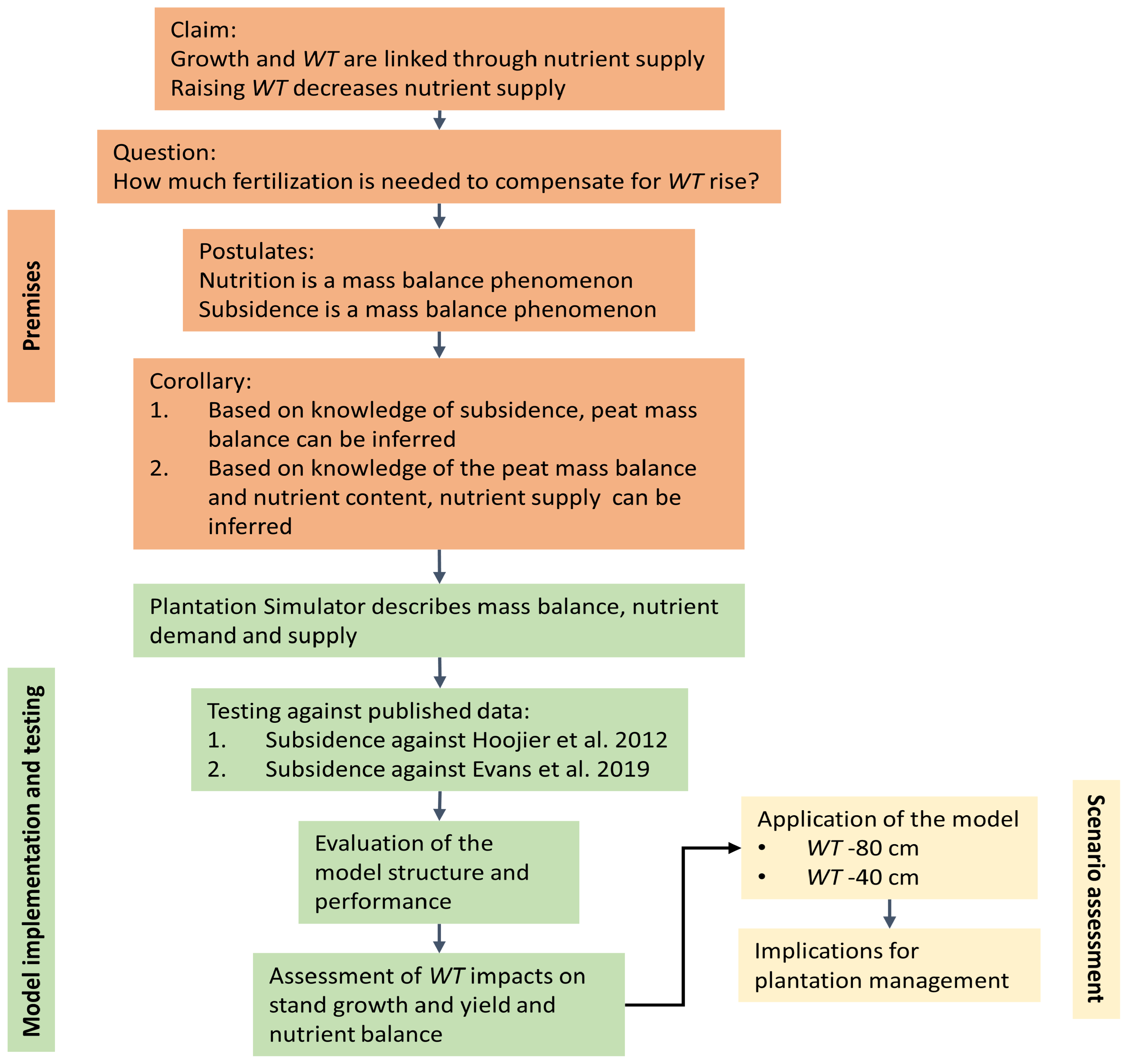
Acacia crassicarpa (Leguminosae) is a fast-growing, nitrogen-fixing tree that is the principal pulpwood plantation species grown on peat soils in SE Asia. It is tolerant of a wide range of soil types and suitable for low fertility sites [23]. The typical plantation rotation period between planting of tree seedlings to harvest, is four to five years, and a closed canopy develops at around 12 to 18 months. Tree height at harvest is in the range from 19 to 24 m. In order to provide suitable rooting conditions, peatland plantations are drained by a network of canals, typically 5 to 8 m wide and 500 to 800 m apart, and by smaller field drains. One dose of artificial P fertilizer is applied at the time of planting [24]. Weeding occurs several times before canopy closure and at two years of age any self-seeded or invasive tree species are removed from the plantation.

2.2. Study Outline

The Plantation Simulator is based on a mass balance (biomass, C, N, P, K) computation of drained tropical peatland. We explicitly account for organic matter produced by the plantation, returned to soil as litter, and decomposed and lost as CO₂ efflux to the atmosphere. The processes driving the mass balance are complex, and comprehensive experimental data for model validation are not available due to confidentiality of data owned by plantation companies. Therefore, the model is tested against published data and by filling the data gaps with required assumptions. First, the overall model structure is described (detailed description in Appendix A), then the model performance in mass balance calculation is shown against published subsidence data. Because the subsidence reports contain little information about the stand properties and dynamics, we used a Monte Carlo approach, deriving unknown site properties from a probability distribution and computing a large simulation set. The results of the simulation set were compared to available independent, published subsidence data sets from similar land use, climatic conditions and peat formations [5,9]. Subsidence is a suitable variable for model testing because it integrates input and output of organic matter through a long time period, whereas direct measurements of the C balance of tropical peatlands are limited to a very small number of shorter-term studies. After having demonstrated plausibility from the mass balance viewpoint, the nutrition simulation results were evaluated against known fertilization schemes. Thereafter, the model was applied for two WT schemes, and the nutritional consequences of the different WT were identified (Figure 1).

2.3. Overall Model Description

The Plantation Simulator describes an Acacia plantation as a system composed of tree stand, soil, nutrient, and hydrology modules (Figure 2). Basic plantation inventory data such as tree species, planting density, site index describing the growth potential of the site [25], and literature-derived parameters are required as inputs for the model. Aspects of the plantation management regime including weeding, and fertilization are given as input parameters to the simulation. The Plantation Simulator computes growth and yield of the Acacia stand, organic matter decomposition and stand nutrition and allows quantification of the impact of plantation management and drainage on these processes. A one-month time step is used. A recursive loop returns information concerning decision criteria, i.e., production, carbon and nutrient balance and peat subsidence, to the model user, thereby enabling adjustment of management procedures in support of improved production and environmental management practices (Figure 2). A detailed model description is provided in the Appendix A.

2.4. Deduction with Plantation Simulator

The key output of the Plantation Simulator is a detailed dynamic nutrient balance (Appendix A.5.3) of the Acacia stand. The balance contains N, P and K demand (Appendix A.5.1) and supply (Appendix A.5.2) as monthly values. Nutrient demand and supply are calculated independently; therefore, the results of growth and yield are conditional on nutrient supply: Following the Liebig’s law of the minimum, growth can occur only if enough resources are available. Using the nutrient balance, the plantation managers can identify which nutrient is needed and when and can construct a fertilization regime to sustain the maximal growth.

Nutrient demand (Appendix A.5.1) is calculated from stand growth (Appendix A.1.1) and litter production (Appendix A.2). Net nutrient demand is derived from nutrient concentrations and growth of Acacia biomass components: foliage, bark, branch, fis, coarse roots, and stem wood (Figure 3). Thereafter, the gross total nutrient demand is calculated as the sum of the net demand and the nutrients lost through monthly litterfall. The competing nutrient demand of weeds is calculated accordingly.

The Plantation Simulator accounts for the main nutrient sources: Retranslocation from senescing litter, atmospheric deposition, nutrient release from decomposition of stand and weed litter, coarse woody debris and peat, and nutrient dissolution from fertilizers. Leguminous atmospheric N-fixation is also considered for Acacia. Each component in the demand and supply can be followed separately, thereby facilitating distinction of the most important processes and detailed component-wise consideration of uncertainty. Nutrient balance is calculated as both cumulative and instantaneous monthly values. The cumulative balance is used if we can assume that all released nutrients are stored in the root zone and are available for plant uptake; whereas the instantaneous balance is valid under the assumption that only nutrients released in the current time step are available for uptake. Cumulative and instantaneous balances represent extreme ends of the uptake scenarios; therefore, interpretation of the results should rely on both balances. The cumulative and instantaneous nutrient balances (Appendix A.5.3) are calculated on an area-based nutrient supply implying that each square meter of the compartment is equally relevant as a nutrient source for a tree. This holds well for a mature plantation with a closed canopy but is not valid for the initial plantation stage when tree seedlings have small root systems. Therefore, we also calculate a tree-wise nutrient balance, which takes account of the area from which a tree can extract nutrients. This is dependent on the canopy size (Figure 4). After the canopy closure the tree-wise nutrient balance equals to the stand nutrient balance, but before the closure the tree-wise balance leads to nutrient deficiency more easily than the stand-wise nutrient balance.

2.5. Model Testing

We used the data presented by Hoojier et al. [5] and Evans et al. [9] to test the performance of the Plantation Simulator. Table 3 in Hoojier et al. [5] presents the mean and standard deviation of WT and subsidence from 21 Acacia crassicarpa sites located on peatlands in Riau, Indonesia. The paper contains, without a specified location, the mean and standard deviation of the peat bulk density, and a record that the bulk density increases by 45 kg m⁻³ in 15 years. Evans et al. [9] present a uniquely large dataset of peat subsidence with respect to mean WT (see Figure 2 in [9]). However, this paper does not contain information about the peat bulk density; we therefore derived the value for initial bulk density from older plantation reported in [5].

Neither of the studies give explicit information about the tree stand nor its development. We simulated the Acacia stand dynamics using the growth and yield model for Acacia mangium [26,27], assuming a constant rate of mortality, and adjusted the dominant height development. Classically the rotation length is set to the age when the mean annual increment (MAI) and the current annual increment (CAI) of the stand intersect. We adjusted the dominant height model parameter values so that they give a height of 21 m (typical height of harvestable stand) at the age of 5 years and produce an intersection of MAI and CAI between the ages of 4 and 5 years. The growth and yield model and its parameterization are presented in detail in the Appendix A.1.1 and Appendix A.1.2.

Nutrient demand and litter production depend on how trees allocate biomass to bark, branches, foliage, roots and stems as all these components have distinctively different nutrient contents. A full set of allometric equations for all these biomass components are not, to our knowledge, publicly available for Acacia crassicarpa. Therefore, we composed the allometric functions calculating the aboveground biomass function specially made for A. crassicarpa [28] and then assuming that biomass is distributed among the components as described by Krisnawati et al. [29] for A. mangium. A more detailed description of the procedure, the biomass equations and parameters are presented in Appendix A.2.

A Monte Carlo simulation set was conducted to fill the data gaps with plausible site and stand characteristics. We lifted parameter values from normal distribution with given mean and standard deviation (

Table 1. Mean and standard deviation (in brackets) of the parameters in the Monte Carlo simulations. Normal distributions were assumed for all variables except mortality rate, which was assumed to have a uniform distribution.

	Hoojier et al. [5]	Evans et al. [9]
Number of sites	21	210
Number of runs per site	50	50
Rotation length, yrs	5	5
Number of rotations	3	3
Site index	20 (3.5)	20 (3.5)
Mortality rate, stems month−1	range 1…20	range 1…20
Initial bulk density, kg m3	89 (18)	110 (22)
WT	as reported	as reported

). For mortality rate we assumed a uniform distribution. We ran the model for 15 yrs, i.e., three full rotations. A monthly WT record was generated from the reported mean WT and assuming 20% standard deviation from the mean with annual dry/wet season cycle [5]. Because each simulation starts from planting, all the stands at a given time point are of equal age, unlike in the measured subsidence dataset. Therefore, a random 10 yrs subset of the simulation results was taken to ensure that the results are independent of the stand age, and thus comparable to the reported field subsidence data. The simulated subsidence accounts for the peat surface elevation change resulting from the simulated decrease in soil organic matter stock, long-term compaction, and short-term shrinking and swelling caused by WT fluctuation. A detailed description of the subsidence calculation is given in the Appendix A.3.4. The overall ecosystem C balance was calculated as the C storage change in soil and the change in stand above-ground biomass C, excluding the commercially usable stems (Appendix A.3.5).

After demonstrated plausibility from the mass balance viewpoint we constructed the N, P and K balance for each simulation and identified the adequacy of nutrient supply with respect to the stand nutrient demand. The timing and quantity of nutrient deficiency was recorded, and the need for fertilization was identified. The effects of each of the input variables in the Monte Carlo simulation (site index, mortality rate, peat bulk density and mean WT) on the subsidence rate, P balance and C balance were assessed using frequency distribution plots.

2.6. Scenario Assessment

The parameterized and tested model was applied for two WT schemes which describe the effects of a change in WT from a mean depth of −0.80 m observed by Jauhiainen et al. [7] for Acacia plantation to a mean of −0.40 m, based on the Indonesian government regulation (SK.22/PPKL/PKG/PKL.0/7/2017). The nutritional consequences of raising the WT were identified. To cover different site and stand characteristics, we ran 200 simulations with varying site index, mortality rate and peat bulk density for low (mean WT−0.8 m) and high WT (mean WT−0.4 m) scenarios. Consequences for stand subsidence, C balance and fertilizer need were quantified.

3. Results

3.1. Testing the Mass Balance Using Published Subsidence Data

The Plantation Simulator successfully predicted both the mean and the range of the peat subsidence in an Acacia plantation, based on standard plantation water and stand management practices (Figure 5). The simulation set shows that the model satisfactorily covers the variation in the Hoojier et al. [5] dataset, which included detailed site-specific input data. However, the model missed the extremes in the Evans et al. [9] dataset, where considerably less input information was provided. In both cases, the mean subsidence was remarkably well predicted. In the simulation set the unknown site variables (site index, mortality rate and peat bulk density) were lifted from probability distributions, which propagates variation into the model target variables as described in Figure 6. Subsidence rate was correlated with WT and with initial peat bulk density. The good match between the measured and modelled subsidence provides a plausible basis for the nutrient balance calculation, because the nutrient dynamics in deep-peat sites depend on the same biogeochemical processes as the mass balance dynamics reflected by the subsidence.

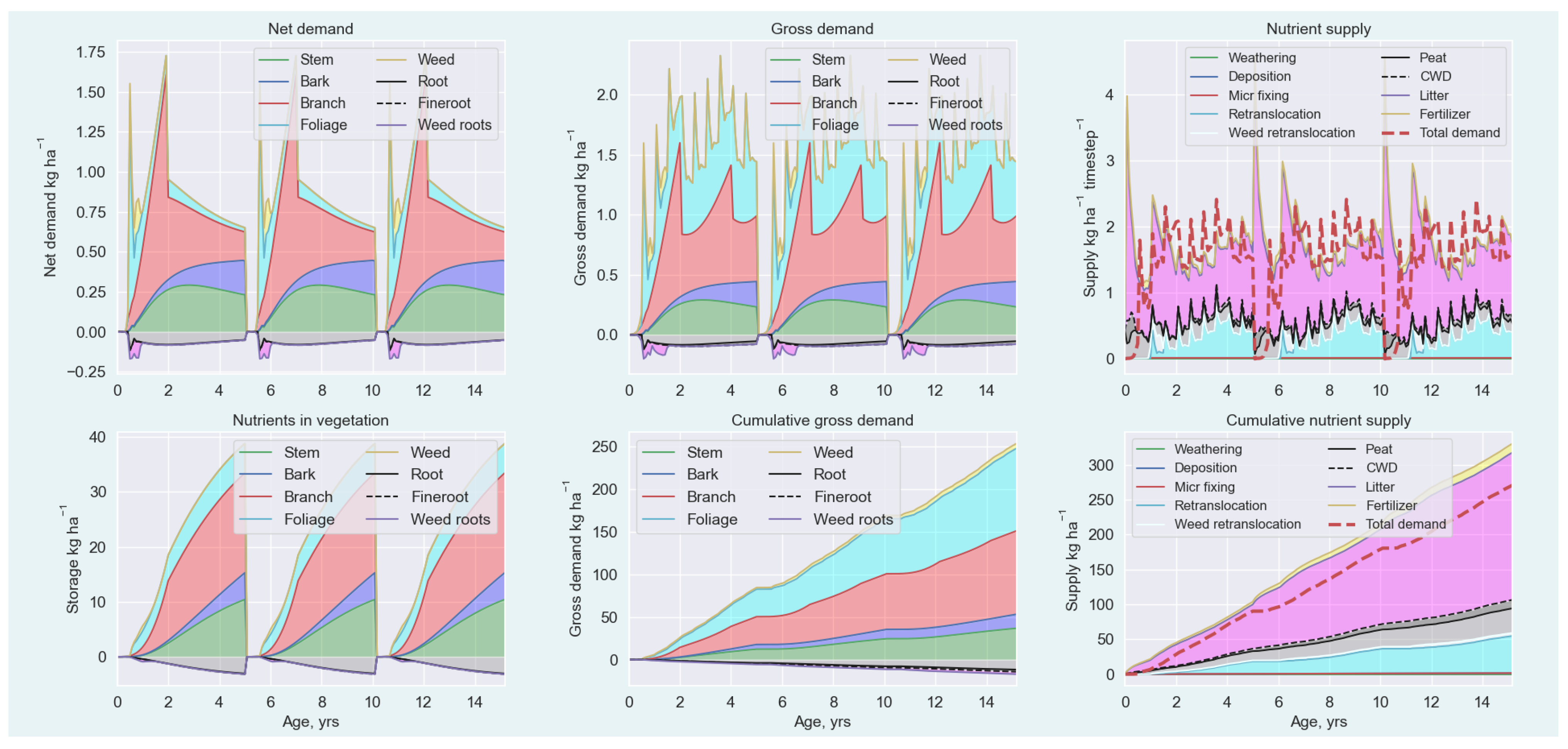
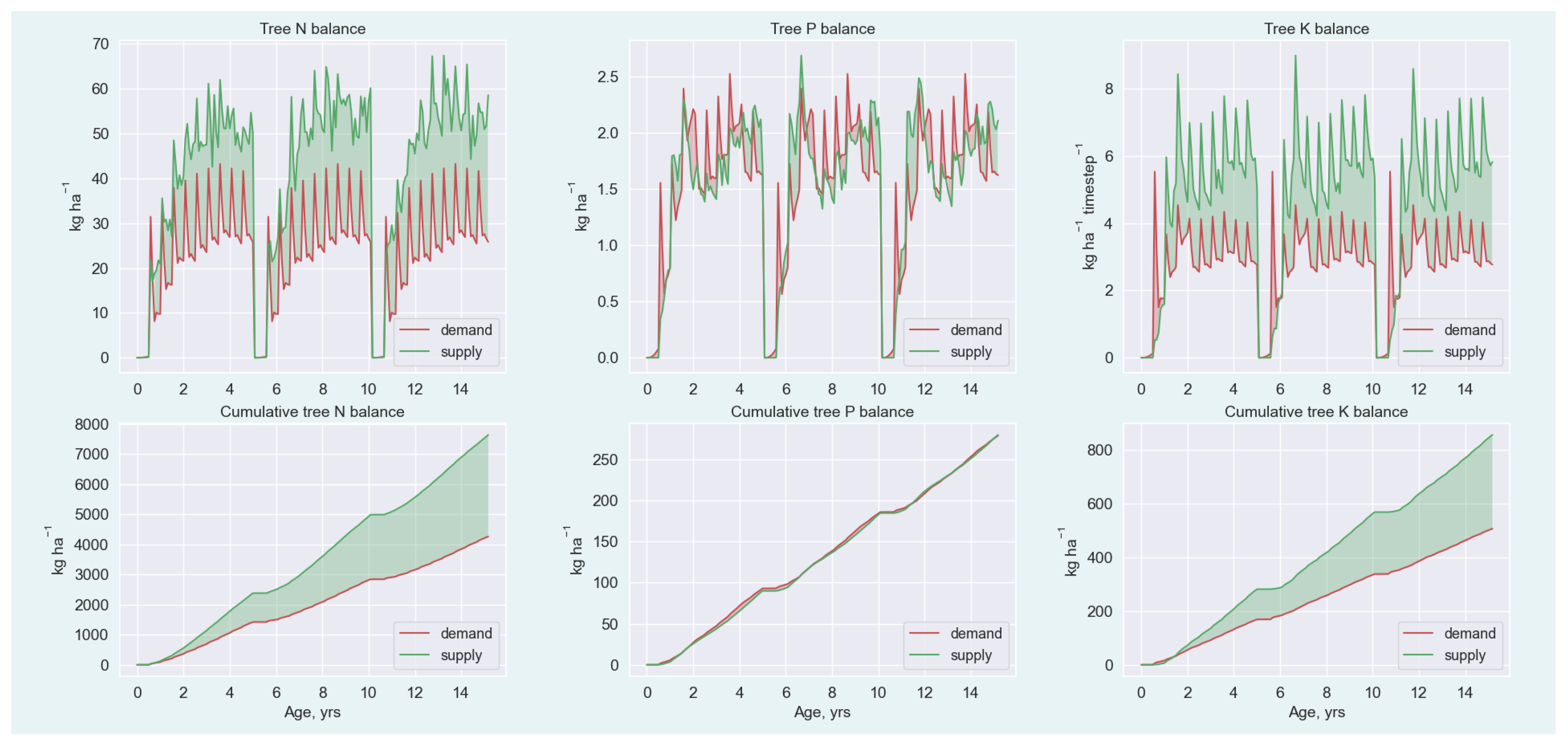
3.2. Nutrient and C Balances

Stand and tree-wise N, P and K balances were extracted from the Monte Carlo simulations based on the Evans et al. [9] dataset (Figure 7). The results indicate a large variation in the nutrient balances. With standard plantation management practices, N and K supply were mainly adequate for production of plantation biomass. In contrast, P supply is likely to be the growth limiting factor. On average, P demand and supply were equal but in half of the cases P balance was negative (Figure 7b,e). Site index, mortality rate and WT affected the P balance (Figure 6 e,f,h). Increasing nutrient demand with increasing site index led to a more negative P balance. The positive correlation between P balance and mortality rate indicates decreasing competition for nutrient resources with increasing mortality. However high mortality opens gaps in the stand and allows nutrient uptake by ground vegetation, which can depress P balance in the highest mortality rates (Figure 6f). Higher WT tended to have a negative impact on P balance but a positive impact on C balance (Figure 6h,l).

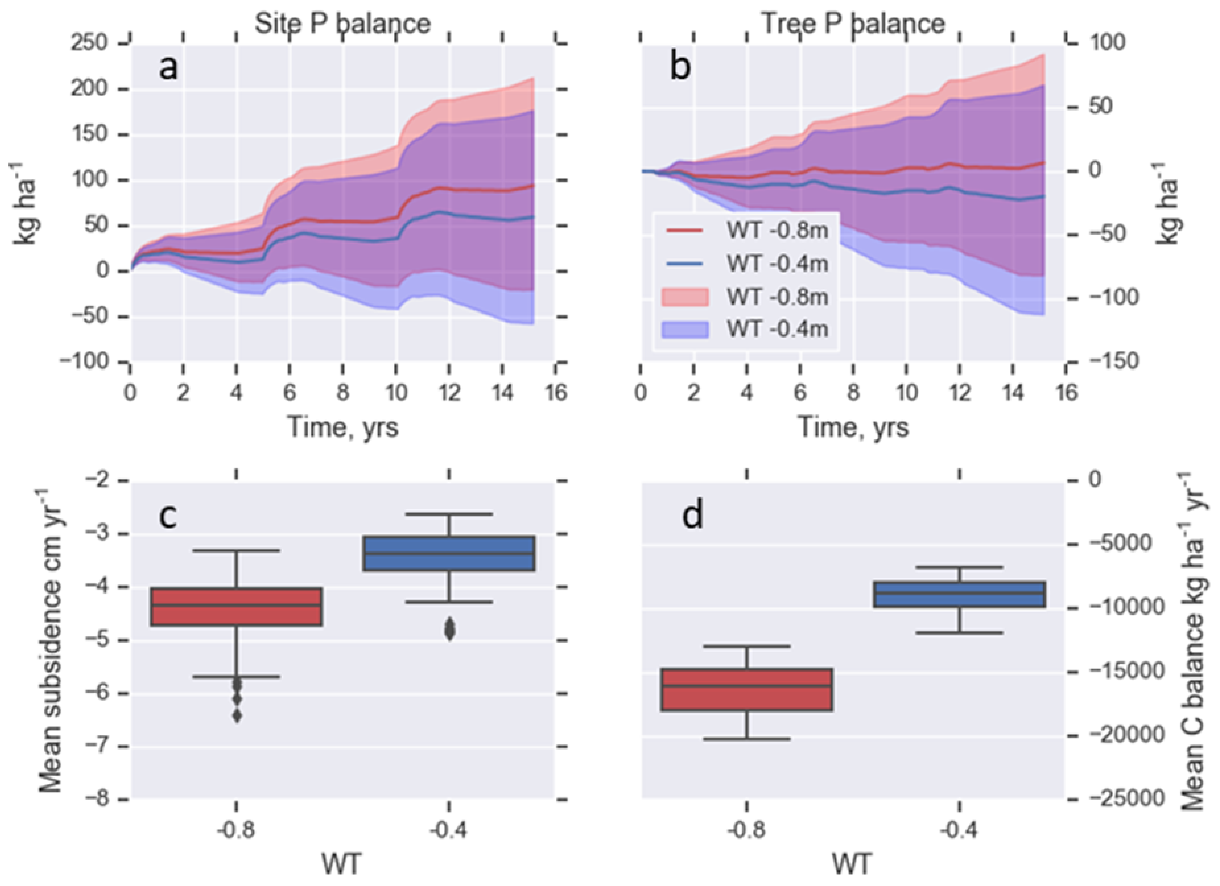
3.3. Scenario Assessment: Raising the Water Table

We applied the Plantation Simulator to identify the nutrient balance change caused by raising WT from a mean of −0.80 m to −0.40 m. Here we concentrate on P, because it was identified to be the main growth limiting nutrient. The cumulative stand-wise P balance remained positive, but decreased by 50 kg ha⁻¹. The tree-wise cumulative P balance changed from being marginally positive (5 kg ha⁻¹) to negative (−17 kg ha⁻¹), implying that the internal supply of P from peat mineralization and nutrient recycling would not be sufficient to achieve the rates of tree growth assumed in the simulation (Figure 8a,b). Under the −0.40 m scenario, it would therefore be necessary to close this nutritional gap, of an estimated 10 to 17 kg P ha⁻¹ rotation⁻¹, with increased fertilization. On the other hand, raising the WT reduced subsidence from 4.4 cm yr⁻¹ to 3.3 cm yr⁻¹ (Figure 8c), and reduced carbon loss from 17 to 9 Mg ha⁻¹ yr⁻¹ (Figure 8d).

4. Discussion

4.1. Need for a Simulation Model

Rates of nutrient consumption are high in tropical short rotation tree plantations, and there is a risk that this could lead to the long-term depletion of soil nutrient resources [24]. This risk is exacerbated for pulpwood plantations that are typically located on infertile soils, and better understanding of the nutrient balance of these systems is therefore needed [30]. Complete nutrient balance studies for tropical plantations are scarce, with most studies dealing only with single nutrients, and focused on mineral soil sites [24,31]. Nutritional issues in plantations growing on peatlands are therefore poorly understood. Subsidence rates in drained tropical peatlands are high, typically 3–5 cm yr⁻¹ [9]. Considering that plantation drainage depths are adjusted over time to maintain a constant WT relative to the peat surface, and that root layer thickness is constant, this continuously exposes “new” organic matter reservoirs to decomposition and nutrient release, but with a high environmental cost. Raising WT decreases peat oxidation and subsequently limits the organic matter decomposition and subsidence, but at the same time reduces the supply of nutrients from decomposing peat [22] which may lead to stand nutrient limitation.

Managing plantations on peat to balance this trade-off between stand productivity and environmental sustainability requires a holistic approach to nutrient management that considers both anthropogenic and natural processes, and the effects of plantation management on these. Therefore, nutrient management of a plantation should incorporate water management, fertilization, weeding, litter and slash management including debarking of harvested stems, and evaluation of nutrient export with harvested biomass (e.g., [30,32]). The Plantation Simulator incorporates these activities within an integrated biogeochemical model that makes visible the different nutrient sources, such as internal translocation of nutrients, circulation of nutrients from litter back to the stand, competition by weeds, and fertilization (see Figure 3). By linking multiple nutrient cycles the model can identify limiting nutrients for growth, helping to focus on nutrient management practices, as argued by Mendham and White [24], and to optimize fertilizer use in order to minimize the associated environmental and economic costs.

A further strength of the Plantation Simulator is that it provides a causal explanation for subsidence, extending empirical studies in which subsidence is predicted solely as a function of WT [5,7,9]. Therefore, it enables a search for optional management schemes connected to combinations of WT control, fertilization, slash management, planting density, and weeding that all affect the nutrient and mass balance and thus help to maximise stand productivity whilst minimizing subsidence and associated CO₂ emissions. Compared to other plantation models [23,24,25,26], Plantation Simulator succeeds to introduce critical characteristics of peatland plantation production into the simulation, such as P and K balance, the role of peat and other organic matter decomposition in the nutrient supply, and the specific the environmental problems, including subsidence and elevated C emissions.

4.2. Model Performance

In the test runs, the Plantation Simulator was able to replicate both the mean and the range of peat subsidence in a tropical pulpwood plantation. With the given range of inputs, the model produced subsidence rates ranging from 2.0 to 8.2 cm yr⁻¹. This covers the previously reported peat subsidence rates for tropical plantations [5,9,33,34]. According to experimental studies, the aboveground biomass in a mature A. crassicarpa stand can vary from 51 to 81 Mg ha⁻¹ [35] or 63 ± 8.3 Mg ha ⁻¹ [28]. Using the Plantation Simulator and applying the mean site index (21 m) and mortality rate (9 stems ha⁻¹ month⁻¹), we obtained a mean above ground biomass of 66 Mg ha⁻¹ at maturity, very close to the reported biomass values. The good fit between the observed and modelled subsidence and biomass accumulation suggest that the stand mass balance is plausibly described and allows us to proceed to an assessment of nutrient balances (Figure 1).

The Evans et al. [9] subsidence dataset represents stand mass balance under normal plantation management, where the mean WT was managed at −0.7 m during the monitoring period that extended up to 10 years. In the long run, site productivity reflects a balance between growth resource supply and demand; thus, the growth of biomass is scaled according to the supply of the minimum growth factor following Liebig’s law of the minimum [25]. Figure 7 clearly suggests that N and K supply are adequate, while P is growth limiting. P shortage was evident during the first three years of the rotation. This is likely due to the competition with weeds, small root systems in the early development of the stand, and a delay between litter fall and nutrient release from the stand litter [24,36]. This finding fits well with the current plantation fertilization practice, which has demonstrated the benefits of P fertilization at time of planting [24,30]. Bich et al. [37] emphasise the importance of P fertilization in Acacia plantations as it enhances microbial activity, decomposition rate, and microbial N fixation.

4.3. Scenario Assessment

When WT is raised, the model shows that nutrient supply from the decomposing peat is considerably reduced, and the stand growth finds, without compensating fertilization, a new equilibrium at lower growth level. In our scenarios, the mean WT was raised from −0.80 m (mean in [7]) to −0.4 m, reflecting recent Indonesian government regulations. The gap between the scenarios in P balance varied from 10 kg ha⁻¹ rotation⁻¹ to 17 kg ha⁻¹ rotation⁻¹ (Figure 8a,b). According to Mendham et al. [32] a universal P dose of 10 kg ha⁻¹ is recommended in the planting of A. mangium in South Sumatra. Assuming that a similar dose is applied to A. crassicarpa, this suggests that (at most) compensation of the raised WT would require a doubling of the current fertilization rate.

4.4. Uncertainty

Each module of the Plantation Simulator contains different levels of uncertainty. The growth and yield module (Appendix A.1.1) represents a traditional whole-stand model, where the stand growth is driven by H_dom and diameter distribution change. Even though currently tree-level growth and yield models are preferred due to their flexibility, stand level models are still suitable for modelling singe-species and even-aged stands [38], such as pulp wood plantations. In this application we could not use the experimentally derived growth and yield parameters for A. crassicarpa because of the confidentiality of plantation company data. Instead we modified parameter values using those reported for A. mangium [26,27] with the exception that the H_dom parameters ($b_{11}$ and $b_{12}$,

Table A1. Variables and parameters in the growth and yield module of the Plantation simulator.

Symbol	Description	Unit	Value
$N_{ini}$	Initial stocking	stems ha−1	1666
$S_I$	Site index	m at $A_{ind}$	17…25
$M_r$	Mortality rate	stems ha−1 yr−1	12…240
$N_s$	Stocking	stems ha −1	500…1666
A	Stand age	yrs	0…5
$H_{dom}$	Dominant height	m	0…25
G	Basal area	m2 ha−1	0…25
$d_{wmean}$	Weighted mean diameter	cm	0…25
$d_{dist}$	Diameter distribution	$N_s$ in diameter d	-
$A_{ind}$	Index age	yrs	5
d	Tree diameter	cm	0…40
h	Tree height	m	0…30
$b_{21}$	$H_{dom}$ parameter	-	0.5
$b_{22}$	$H_{dom}$ parameter	-	1.1
$b_{30}$	G parameter	-	−4.14724
$b_{31}$	G parameter	-	−2.07358
$b_{32}$	G parameter	-	0.99584
$b_{33}$	G parameter	-	0.62386
$b_w$	Diameter disrtibution parameter	-	Equation (A5)
$c_w$	Diameter disrtibution parameter	-	Equation (A6)
$b_{50}$	Diameter disrtibution parameter	-	0.00378
$b_{51}$	Diameter disrtibution parameter	-	1.06688
$b_{52}$	Diameter disrtibution parameter	-	0.09209
$b_{60}$	Diameter disrtibution parameter	-	1.49093
$b_{61}$	Diameter disrtibution parameter	-	−0.03053
$b_{80}$	Tree height parameter	-	−0.5929
$b_{81}$	Tree height parameter	-	−0.31894
$b_{82}$	Tree height parameter	-	1.48904
$b_{90}$	Tree height parameter	-	6.77843
$b_{91}$	Tree height parameter	-	−0.13929
$b_{92}$	Tree height parameter	-	0.2971
$b_{93}$	Tree height parameter	-	−0.72857
$b_{100}$	Tree height parameter	-	Equation (A8)
$b_{101}$	Tree height parameter	-	Equation (A9)
$b_{110}$	Tree volume parameter	-	−9.83466
$b_{111}$	Tree volume parameter	-	1.70518
$b_{112}$	Tree volume parameter	-	1.14496

) were adjusted so that the production scheme became realistic in terms of rotation time. While we are unable to rigorously evaluate how well these parameters fit for A. crassicarpa in the absence of direct observations, we did find that the simulation as a whole produced plausible results. Omitting the parameterization problem, the growth and yield module per se contains rather low uncertainty, as the growth is easily verifiable using standard plantation inventory data. Thereafter, the relevant parameters affecting mortality rate, height, basal area and diameter development, can be easily modified accordingly. This is typically the first step in the application of the Plantation Simulator.

Biomass models (Appendix A.2) are usually based on much smaller datasets than growth and yield models, because measurement of biomass components is laborious [38]. Therefore, uncertainty of the biomass module may be slightly higher than that in the growth and yield module, although the allometric relationships within two stands of the same species tend to be rather stable if the stand density is similar [25]. This is particularly true for plantations with controlled genetic material and standardized stand management practices. It is clear, however, that a species-specific additive biomass model that includes bark, branch, foliage, roots and stems for A. crassicarpa would improve the accuracy of the nutrient balance estimates.

Decomposition is an essential part of nutrient cycling [30], and a major source of nutrients in drained deep peat sites. Decomposition of organic matter is a complex phenomenon, where not only original substances decompose, but also new substances are generated [39]; therefore, process-based decomposition models typically have rather a large uncertainty if site-specific input data are limited [40]. The Plantation Simulator considers separately decomposition and storage for $CWD$ (Appendix A.3.1), stand litter (Appendix A.3.2) and peat (Appendix A.3.3). $CWD$ model [41] applies empirical approach where the decomposition rate depends on mean air temperature, stem diameter and initial wood density. Stand litter is decomposed using the mechanistic Romul model [42]. An empirical carbon emission function determined for Acacia plantations in tropical peatlands was used to estimate the total decomposition including all organic matter components [7]. To allocate decomposition to $CWD$, stand litter and peat, we subtracted the calculated C emissions of $CWD$ model and Romul model from the total C emission. The remaining emission represented the peat decomposition. This structure decreases uncertainty of the decomposition module as a whole, because it frames the total decomposition closely to the range observed by Jauhiainen et al. [7] for A. crassicarpa plantation on tropical peat and in the same area.

Nutrient demand module (Appendix A.5.1) contains less uncertainty than the nutrient supply module (Appendix A.5.2), because nutrient demand is closely related to stand development. A simulation with site index (21 m) and mortality rate (9 stems ha⁻¹ month⁻¹), shows that two thirds of the P uptake ends up in foliage and branches. This emphasizes the importance of leaving logging residues on site after harvesting [37]. In our application the litterfall rate is estimated based on the longevity of each biomass component, with parameters based on expert knowledge. The strength of this approach is that the litter production follows the growth and biomass component models and all components will eventually be transferred to litter. This narrows down the uncertainty range. Nutrient supply from the decomposing stand litter and from decomposing peat were the main sources of P supply contributing three quarters of the cumulative P supply during one rotation. The uncertainties in the decomposition models propagate to the nutrient supply estimates.

In this application C balance was calculated as a C storage change in soil and biomass, but omitting the contribution of stems, which are used for pulp production. Thus, the C balance includes biomass of weeds and unmerchantable parts of trees, and subsequently provides a C balance estimate coherent to our mass balance approach. The IPCC emission factors for tropical Acacia plantation on drained peatland are based on soil C storage change (−25 to −15 Mg CO₂-C ha⁻¹ yr⁻¹), equivalent to 15 to 25 Mg CO₂-C ha⁻¹ yr⁻¹ of emission [5,7,43,44]. In our estimates that account for the unmerchantable parts of trees, the balance varied between −20 and −10 Mg CO₂-C ha⁻¹ yr⁻¹ (Figure 6i) indicating a slightly smaller C source than the IPCC values. Using the Plantation Simulator and applying the mean site index (21 m), mortality rate (9 stems ha⁻¹ month⁻¹), and mean WT of −0.8 m, the C balance accounting only for soil Equation (A32) was −19 Mg CO₂-C ha⁻¹ yr⁻¹, omitting the stems Equation (A33)-14Mg CO₂-C ha⁻¹ yr⁻¹ and including the stems Equation (A34) −11 Mg CO₂-C ha⁻¹ yr⁻¹. The C balance estimates can be considered realistic, and therefore the Plantation Simulator can be a useful tool in producing more accurate net C emission estimates, because it takes into account the effect of stand properties, as well as stand and WT management. Future development of Plantation Simulator includes incorporation of hydrology, photosynthesis and net primary production modules to the model, and changing from stand-based to grid-based solution to facilitate simultaneous simulation of large areas.

References

1. Nichols, J.E.; Peteet, D.M. Rapid expansion of northern peatlands and doubled estimate of carbon storage. Nat. Geosci. 2019, 12, 917–921. [Google Scholar] [CrossRef]
2. Dargie, G.; Lewis, S.; Lawson, I.; Mitchard, E.; Page, S.; Bocko, Y.; Ifo, S. Age, extent and carbon storage of the central Congo Basin peatland complex. Nature 2017, 542, 86–90. [Google Scholar] [CrossRef]
3. Reddy, K.; Delaune, R. Biogeochemistry of Wetlands: Science and Applications; CRC Press: Boca Raton, FL, USA, 2008; pp. 1–781. [Google Scholar] [CrossRef]
4. Minkkinen, K.; Laine, J. Long-term effect of forest drainage on the peat carbon stores of pine mires in Finland. Can. J. For. Res. 1998, 28, 1267–1275. [Google Scholar] [CrossRef]
5. Hooijer, A.; Page, S.; Jauhiainen, J.; Lee, W.A.; Lu, X.X.; Idris, A.; Anshari, G. Subsidence and carbon loss in drained tropical peatlands. Biogeosciences 2012, 9, 1053–1071. [Google Scholar] [CrossRef] [Green Version]
6. Ojanen, P.; Minkkinen, K.; Alm, J.; Penttilä, T. Soil–atmosphere CO2, CH4 and N2O fluxes in boreal forestry-drained peatlands. For. Ecol. Manag. 2010, 260, 411–421. [Google Scholar] [CrossRef]
7. Jauhiainen, J.; Hooijer, A.; Page, S.E. Carbon dioxide emissions from an Acacia plantation on peatland in Sumatra, Indonesia. Biogeosciences 2012, 9, 617–630. [Google Scholar] [CrossRef] [Green Version]
8. Miettinen, J.; Shi, C.; Liew, S.C. Fire Distribution in Peninsular Malaysia, Sumatra and Borneo in 2015 with Special Emphasis on Peatland Fires. Environ. Manag. 2017, 60. [Google Scholar] [CrossRef] [PubMed]
9. Evans, C.D.; Williamson, J.M.; Kacaribu, F.; Irawan, D.; Suardiwerianto, Y.; Hidayat, M.F.; Laurén, A.; Page, S.E. Rates and spatial variability of peat subsidence in Acacia plantation and forest landscapes in Sumatra, Indonesia. Geoderma 2019, 338, 410–421. [Google Scholar] [CrossRef]
10. Nieminen, M.; Sallantaus, T.; Ukonmaanaho, L.; Nieminen, T.M.; Sarkkola, S. Nitrogen and phosphorus concentrations in discharge from drained peatland forests are increasing. Sci. Total. Environ. 2017, 609, 974–981. [Google Scholar] [CrossRef]
11. Konecny, K.; Ballhorn, U.; Navratil, P.; Jubanski, J.; Page, S.E.; Tansey, K.; Hooijer, A.; Vernimmen, R.; Siegert, F. Variable carbon losses from recurrent fires in drained tropical peatlands. Glob. Chang. Biol. 2016, 22, 1469–1480. [Google Scholar] [CrossRef] [Green Version]
12. Page, S.; Rieley, J.; Banks, C. Global and regional importance of the tropical peatland carbon pool. Glob. Chang. Biol. 2011, 17, 798–818. [Google Scholar] [CrossRef] [Green Version]
13. Miettinen, J.; Shi, C.; Liew, S.C. Land cover distribution in the peatlands of Peninsular Malaysia, Sumatra and Borneo in 2015 with changes since 1990. Glob. Ecol. Conserv. 2016, 6, 67–78. [Google Scholar] [CrossRef] [Green Version]
14. Wijedasa, L.; Jauhiainen, J.; Könönen, M.; Lampela, M.; Vasander, H.; Leblanc, M.C.; Evers, S.; Smith, T.; Yule, C.; Varkkey, H.; et al. Denial of long-term issues with agriculture on tropical peatlands will have devastating consequences. Glob. Chang. Biol. 2017, 23. [Google Scholar] [CrossRef] [PubMed] [Green Version]
15. Finér, L. Biomass and nutrient dynamics of Scots pine on a drained ombrotrophic bog. Finn. For. Res. Inst. Res. Pap. 1992, 420, 1–43. [Google Scholar]
16. Lauhanen, R.; Kaunisto, S. Effect of drainage maintenance on the nutrient status on drained Scots pine mires. Suo 1999, 50, 119–132. [Google Scholar]
17. Silvola, J. Effect of drainage and fertilization on carbon output and nutrient mineralization of peat. Suo 1988, 1–2, 27–37. [Google Scholar]
18. Wang, M.; Talbot, J.; Moore, T.R. Drainage and fertilization effects on nutrient availability in an ombrotrophic peatland. Sci. Total. Environ. 2018, 621, 1255–1263. [Google Scholar] [CrossRef]
19. Kaunisto, S.; Paavilainen, E. Nutrient stores in old drainage areas and growth of stands. Comminicationes Inst. For. Fenn. 1988, 145, 1–39. [Google Scholar]
20. Laiho, R.; Laine, J. Nitrogen and phosphorus stores in Peatlands drained for forestry in Finland. Scand. J. For. Res. 1994, 9, 251–260. [Google Scholar] [CrossRef]
21. Sarkkola, S.; Ukonmaanaho, L.; Nieminen, T.; Laiho, R.; Laurén, A.; Finér, L.; Nieminen, M. Should harvest residues be left on site in peatland forests to decrease the risk of potassium depletion? For. Ecol. Manag. 2016, 374, 136–145. [Google Scholar] [CrossRef]
22. Marwanto, S.; Watanabe, T.; Iskandar, W.; Sabiham, S.; Funakawa, S. Effects of seasonal rainfall and water table movement on the soil solution composition of tropical peatland. Soil Sci. Plant Nutr. 2018, 64, 386–395. [Google Scholar] [CrossRef]
23. Arnold, R.; Cuevas, E. Genetic variation in early growth, stem straightness and survival in Acacia crassicarpa, A. mangium and Eucalyptus urophylla in Bukbdnon province, Philippines. J. Trop. For. Sci. 2003, 15, 332–351. [Google Scholar]
24. Mendham, D.S.; White, D.A. A review of nutrient, water and organic matter dynamics of tropical acacias on mineral soils for improved management in Southeast Asia. Aust. For. 2019, 82, 45–56. [Google Scholar] [CrossRef] [Green Version]
25. Fabrika, M.; Pretzsch, H. Forest Ecosystem Analysis and Modelling; Technical University in Zvolen, Faculty of Forestry, Department of Forest Management and Geodesy: Zvolen, Slovakia, 2013; pp. 1–620. [Google Scholar]
26. Forss, E.; Gadow, K.; Saborowski, J. Growth models for unthinned Acacia mangium plantations in South Kalimantan, Indonesia. J. Trop. For. Res. 1996, 8, 449–462. [Google Scholar]
27. Forss, E.; Maltamo, M.; Saramäki, J. Static stand and tree characteristics model for Acacia mangium plantations. J. Trop. For. Sci. 1998, 10, 318–336. [Google Scholar]
28. Chen, Y.; Liu, Z.; Rao, X.; Wang, X.; Liang, C.; Lin, Y.; Zhou, L.; Cai, X.a.; Fu, S. Carbon Storage and Allocation Pattern in Plant Biomass among Different Forest Plantation Stands in Guangdong, China. Forests 2015, 6, 794–808. [Google Scholar] [CrossRef] [Green Version]
29. Krisnawati, H.; Kallio, M.; Kanninen, M. Acacia Mangium Willd.: Ecology, Silviculture and Productivity; Center for International Forestry Research: Bogor, Indonesia, 2011. [Google Scholar] [CrossRef]
30. Alvarado, A. Plant Nutrition in Tropical Forestry. In Tropical Forestry Handbook; Pancel, L., Köhl, M., Eds.; Springer: Berlin/Heidelberg, Germany, 2016; pp. 1113–1202. [Google Scholar]
31. Laclau, J.P.; Ranger, J.; Gonçalves, J.; Maquere, V.; Krusche, A.; M’Bou, A.; Nouvellon, Y.; Saint-Andre, L.; Jean-Pierre, B.; Piccolo, M.; et al. Biogeochemical cycles of nutrients in tropical Eucalyptus plantations: Main features shown by intensive monitoring in Congo and Brazil. For. Ecol. Manag. 2010, 259, 1771–1785. [Google Scholar] [CrossRef]
32. Mendham, D.S.; Hardiyanto, E.B.; Wicaksono, A.; Nurudin, M. Nutrient management of contrasting Acacia mangium genotypes and weed management strategies in South Sumatra, Indonesia. Aust. For. 2017, 80, 127–134. [Google Scholar] [CrossRef] [Green Version]
33. Othman, H.; Mohammed, A.; Mohamad Darus, F.; Harun, M.; Zambri, M. Best management practices for oil palm cultivati on peat: Ground water-table maintenance in relation to peat subsidence and estimation of CO2 emissions at Sessang, Sarawak. J. Oil Palm Res. 2011, 23, 1078–1086. [Google Scholar]
34. Couwenberg, J.; Hooijer, A. Towards robust subsidence-based soil carbon emission factors for peat soils in South-East Asia, with special reference to oil palm plantations. Mires Peat 2013, 12, 1–13. [Google Scholar]
35. Ardiansyah, M.; Rusdi, M.; Rosalina, U.; Boer, R. Biomass Estimation and Carbon Stock Calculation in the Industrial Forest Plantation of PT WKS Jambi Using Landsat Data. 2005. Available online: https://www.researchgate.net/profile/Muhammad-Rusdi/publication/279851174_Biomass_estimation_and_carbon_stock_calculation_in_the_industrial_forest_plantation_of_PT_WKS_Jambi_using_Landsat_data/links/559bf03408ae7f3eb4cee337/Biomass-estimation-and-carbon-stock-calculation-in-the-industrial-forest-plantation-of-PT-WKS-Jambi-using-Landsat-data.pdf (accessed on 1 March 2021).
36. Nambiar, S. Management of Soil, Nutrients and Water in Tropical Plantation Forests; ACIAR; CSIRO Australia; CIFOR Indonesia: Canberra, Australia; Bogor, Indonesia, 1997. [Google Scholar]
37. Van Bich, N.; Eyles, A.; Mendham, D.; Dong, T.L.; Ratkowsky, D.; Evans, K.J.; Hai, V.D.; Thanh, H.V.; Thinh, N.V.; Mohammed, C. Contribution of Harvest Residues to Nutrient Cycling in a Tropical Acacia mangium Willd. Plantation. Forests 2018, 9, 577. [Google Scholar] [CrossRef] [Green Version]
38. Weiskittel, A.; Hann, D.W.; Kershaw, J.A., Jr.; Vanclay, J.K. Forest Growth and Yield Modeling; John Wiley & Sons, Ltd.: Hoboken, NJ, USA, 2011; pp. 1–415. [Google Scholar]
39. Berg, B.; McClaugherty, C. Plant Litter. Decomposition, Humus Formation, Carbon Sequestration; Springer: Berlin/Heidelberg, Germany, 2003. [Google Scholar]
40. Hararuk, O.; Smith, M.J.; Luo, Y. Microbial models with data-driven parameters predict stronger soil carbon responses to climate change. Glob. Chang. Biol. 2015, 21, 2439–2453. [Google Scholar] [CrossRef] [PubMed]
41. Mackensen, J.; Bauhus, J.; Webber, E. Decomposition rates of coarse woody debris—A review with particular emphasis on Australian tree species. Aust. J. Bot. 2003, 51, 27–37. [Google Scholar] [CrossRef]
42. Chertov, O.; Komarov, A.; Nadporozhskaya, M.; Bykhovets, S.; Zudin, S. ROMUL—A model of forest soil organic matter dynamics as a substantial tool for forest ecosystem modeling. Ecol. Model. 2001, 138, 289–308. [Google Scholar] [CrossRef]
43. Basuki, S.; Munoz, C.P. Emission of CO2 and CH4 from plantation forest of Acacia crassicarpa on peatlands in Indonesia. In Proceedings of the 14th International Peat Congress, Stockholm, Sweden, 3–8 June 2012; pp. 1–7. [Google Scholar]
44. Warren, M.W.; Kauffman, J.B.; Murdiyarso, D.; Anshari, G.; Hergoualc’h, K.; Kurnianto, S.; Purbopuspito, J.; Gusmayanti, E.; Afifudin, M.; Rahajoe, J.; et al. A cost-efficient method to assess carbon stocks in tropical peat soil. Biogeosciences 2012, 9, 4477–4485. [Google Scholar] [CrossRef] [Green Version]
45. Bi, H.; Turner, J.; Lambert, M. Additive biomass equations for native eucalypt forest trees of temperate Australia. Trees 2004, 18, 467–479. [Google Scholar] [CrossRef]
46. Palviainen, M.; Finér, L. Decomposition and nutrient release from Norway spruce coarse roots and stumps—A 40-year chronosequence study. For. Ecol. Manag. 2015, 358, 1–11. [Google Scholar] [CrossRef]
47. Anonymous. Description and Manual of Romul. Available online: http://xxx.lanl.gov/abs/http://ecomodelling.ru/images/dles/en_romul_description_manual.pdf (accessed on 11 November 2020).
48. Camporese, M.; Ferraris, S.; Putti, M.; Salandin, P.; Teatini, P. Hydrological modeling in swelling/shrinking peat soils. Water Resour. Res. 2006, 42. [Google Scholar] [CrossRef] [Green Version]
Figure 1. Deduction chart of the study.
Forests 12 00312 g001
Figure 2. Structure of the Plantation Simulator. The plantation system (dark grey panel) accounts for growth and yield of the stand, water table and biogeochemical processes within the site, and returns target variable information to the management system. Target variables, i.e., current yield, nutrient status, carbon balance and subsidence rate are evaluated against decision criteria and the management practices can be adjusted to reach better production and environmental targets. Codes A1, A11, A12, etc. refer to chapters in the detailed model description in Appendix A.1, Appendix A.1.1, Appendix A.1.2, etc.
Forests 12 00312 g002
Figure 3. Example of a phosphorus balance of an Acacia stand. Stand P storage (lower left) is computed from the biomass components (bark, branch, foliage, stem, fis, coarse roots) and their nutrient concentrations. Net demand (upper left) is the monthly change in nutrient storage. Gross demand (upper middle) accounts for net uptake and the uptake that replaces the nutrients lost in litterfall. Cumulative gross demand (lower middle) shows that the stand needs P at an approximate rate of 280 kg ha−1 during three rotations (250 kg for above-ground components and 30 kg for the below-ground components shown below the X-axis). The instantaneous nutrient supply (upper right) shows how much P becomes available from internal retranslocation, atmospheric deposition, fertilizer dissolution and decomposition of litter, coarse woody debris and peat. The cumulative nutrient supply is shown in the lower right panel. The dotted red line in the rightmost panels indicates the total nutrient demand of the stand.
Forests 12 00312 g003
Figure 4. Tree-wise nutrient balance for N, P and K. The tree-wise nutrient balance allows us to consider available nutrient reservoirs within the reach of the root system before canopy closure. Therefore, even though the area-based nutrient balance would suggest an adequate nutrient supply, the individual tree might suffer deficiency. The red area between the supply and demand curves indicates deficiency.
Forests 12 00312 g004
Figure 5. Measured (range in purple, mean as dotted line) and modelled subsidence (range in blue, mean as solid black line).
Forests 12 00312 g005
Figure 6. Effect of site index (m at index age of 5 years) (a,e,i), mortality rate (stems ha−1 month−1) (b,f,j), peat bulk density (kg m−1) (c,g,k) and mean WT (cm, positive down) (d,h,l) on annual subsidence rate (cm yr−1) (row 1), tree–wise P balance (kg ha−1) (row 2) and site C balance (kg ha−1 yr−1, negative value indicating C source) (row 3). The figure was constructed from the Monte Carlo simulations using the Evans et al. [9] dataset.
Forests 12 00312 g006
Figure 7. N, P and K balance calculated based on standard plantation management practices, using data from the Evans et al. [9] dataset. The simulation period covers 15 years including three full rotations from planting to harvesting. The upper panels describe the instantaneous stand-wise N (a), P (b) and K (c) balance (difference between nutrient supply and demand), lower panels describe the cumulative tree-wise N (d), P (e) and K (f) balance. Negative values in all cases indicate that nutrient supply is smaller than the demand. The red area shows the range, and the solid black line shows the mean.
Forests 12 00312 g007
Figure 8. (a) Effects of alternative WT scenarios on stand P balance, (b) tree P balance, (c) annual subsidence and (d) C balance (negative value implies C source).
Forests 12 00312 g008