Abstract
The cooling and humidifying effects of urban aggregated green infrastructure can provide essential services for city ecosystems, regulating microclimates or mitigating the urban heat island effect. However, the optimal thresholds of plant community structure parameters for maximizing the associated cooling and humidifying effects remain unclear. In this paper, we use the method of dummy variable regression to measure plant communities in an urban aggregated green infrastructure. By examining the relationships between the cooling and humidifying effects and plant community structure parameters (i.e., canopy density, porosity, and vegetation type), we introduce optimal thresholds for the parameters. We find that canopy density has a significantly positive correlation with both cooling and humidifying effects, while porosity has a positive correlation with cooling and a negative one with humidifying. Different vegetation types have distinct influences on cooling and humidifying effects. When the canopy density is between 0.81 and 0.85 and the porosity is between 0.31 and 0.35, the cooling and humidifying effects of the plant communities reach their peak. Additionally, the greening coverage rate and spatial types of urban aggregated green infrastructure have influences on cooling and humidifying effects. The findings can help us to better understand the relationships between plant community structure parameters and their temperature regulation functioning for urban aggregated green infrastructure. This study provides guidelines and theoretical references for the plant configuration of future urban green spaces.
1. Introduction
The ongoing rapid urbanization has great potential to improve human development. However, urbanization can also lead to severe environmental problems, such as the Urban Heat Island (UHI) effect [1]. A progressive increase in the UHI effect has been observed in both large cities and medium-sized municipalities [2]. This phenomenon has become a widespread concern; thus, the necessity to solve the current problem is urgent. Over the last two decades, studies focusing on mitigating UHI effects have grown steadily [3,4]. These previous studies have shown that urban green infrastructure presents an important approach to mitigate the heat island effect.
In 1995, Forman systematically summarized the methods of landscape pattern optimization, focusing on the overall optimization of landscape pattern [5]. Aggregated green infrastructure includes multiple vegetation types (compared to distributed green infrastructure) and is better able to maintain and protect genetic diversity, providing sustainable ecosystem services. Distributed green infrastructure also has advantages, however, as it takes up less space and can be distributed throughout man-made landscapes, enhancing the landscape diversity and acting as temporary habitats or “stepping stones”. Therefore, the combination of aggregation and distribution is considered a highly irreplaceable landscape pattern for the overall layout. Furthermore, larger green spaces are, on average, cooler than the smaller ones; however, the relationship between size and the local cool-island intensity is likely non-linear. Cao reported that the cooling effect is more significant in large green patches [6], while smaller urban green spaces fail to mitigate “urban heat island” effects. Relevant studies have shown that the threshold value for urban green space with the “urban cold island” effect is 3 hectares, whereas parks smaller than 3 ha were more variable in their temperature, in comparison with their surroundings [7,8]. Therefore, urban green spaces can be divided into aggregated green infrastructure and distributed green infrastructure, according to this threshold. This classification method helps in the study of the correlation between urban green infrastructure scale and urban heat island effect.
Urban aggregated green infrastructure, such as parks of large size, can considerably mitigate the UHI effect through the cooling and humidifying effects exerted by plants [9,10,11,12,13,14,15]. The number of studies regarding the cooling and humidifying effects of plant communities during summer has increased in recent years, raising concerns regarding the following four themes: differences in the cooling and humidifying effects of various plant communities, contrasts in plant community structures, the variety of types of underlying surfaces, and diverse scales of urban green spaces [16]. It is well-known that trees can affect the air temperature and relative humidity through shading, transpiration, and evaporative cooling, so that the effects generated by green belts with trees, shrubs, and grass are more obvious than those of lawns [6,17]. The canopy density and leaf area indices are better for determining the cooling and humidifying effects from 9:00 to 12:00 AM [18]. However, the above research only focused on photosynthesis measurement, based on single leaves [19,20,21,22,23,24], and the actual measurement of environmental factors of green space [25,26,27,28,29], but lacked research on the quantitative relationships between plant community structure parameters and the aggregated green infrastructure [30,31]. Furthermore, most studies have only paid attention to the canopy density index. Three-dimensional research on the cooling effects of green space in vertical and horizontal directions is relatively rare.
Porosity is the projection from the vertical plane of plant community structure. However, at present, little is known about the relationships between the porosity and cooling and humidifying effects; even less is known about thresholds to maximize the cooling and humidifying effects [32]. Thus, we should not only pay attention to the canopy density of the plant community in aggregated green infrastructure, but also to its porosity and the spatial types of the site [33,34]. In this study, we introduce a method combining actual measurements from a plant community with dummy regression analysis, taking the Guishan green space as a typical site and focusing on nine greening vegetation types of the Mingwaiguo scenery zone in Nanjing. Based on structural parameters of the plant community (e.g., canopy density and porosity), we conducted real-time monitoring of the microenvironment temperature and relative humidity, and figured out the range of cooling and humidifying effects generated by the different communities. The detailed experimental steps are shown in Figure 1. This paper mainly answers the following two key questions: (1) What are the optimal thresholds of plant community structure parameters for aggregated green infrastructure, in order to maximize the cooling and humidifying effects? and (2) Which indicators affect the cooling and humidifying effects of the aggregated green infrastructure? In this study, we aim to provide a scientific reference for the vegetation allocation in aggregated green infrastructure construction, in order to reduce the urban heat island effect, and provide quantitative models for efficiency evaluation, in terms of alleviating the heat island effect through aggregated green infrastructure.
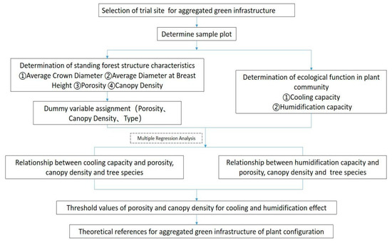
Figure 1.
Experimental method step diagram.
2. Materials and Methods
2.1. Location of Study Area
2.1.1. Study Area
Nanjing, located in the lower reaches of the Yangtze River Delta, has a subtropical monsoon climate, with an average annual rainfall of 117 days (2206.5 mm) and relative humidity of 76%. Its average annual temperature is 15.5 °C. The average temperature in January is 2.3 °C, while that in July is 25.3 °C. In 2015, the number of days that reached the second level of air quality was 235, with a passing rate of 64.4%, while the number of days that failed to reach the second level of air quality was 130. The primary pollution was PM 2.5. The Mingwaiguo scenery zone is the most important structural green space in Nanjing. Its green space layout reflects the characteristics of aggregate-with-outliers. The Guishan green space (coordinates: 118.905469° E, 32.096836° N–118.912763° E, 32.100553° N), with area of about 14 hectares, is located in the demonstration part of the Mingwaiguo scenery zone (Figure 2). The study area is a typical urban aggregated green infrastructure. Along with the construction of large and small Guishan, vegetation types like Magnolia grandiflora, Osmanthus fragrans, and Cerasus were planted in a large amount, with a greening coverage rate of more than 80% (Figure 3). Different types of vegetation form community structures of tree–shrub–herbage, tree–herbage, and different spatial types, such as open space, semi-open space, and closed space (Figure 4). The weather data measured in this area are basically consistent with those at the Nanjing National Benchmark Climate Station (coordinates: 118.910438° E, 31.935088° N).
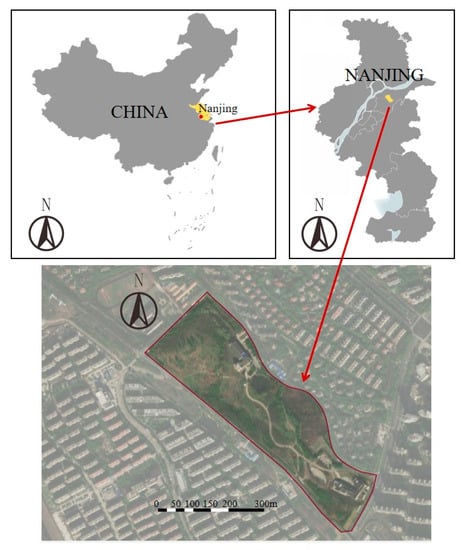
Figure 2.
Map showing the experimental plot area—Guishan—located in the demonstration part of Mingwaiguo scenery zone.
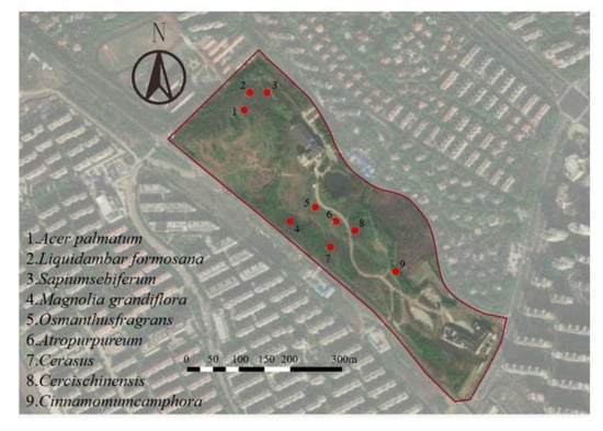
Figure 3.
Sample distribution map.
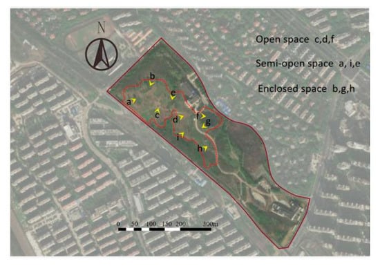
Figure 4.
Spatial type distribution map.
2.1.2. Sample Collection
We selected nine types of single plant communities, which had high representativeness and occurrence frequency in the Mingwaiguo scenery zone, and were of the same age and in good growing conditions. Experimental communities had similar surroundings with the same underlying surface—grass—on the corner, Ophiopogon japonicus, and weeds. The multiple tree species present had multiple characteristics, including tree shape, canopy size and the features of the tree leaves. Experimental design covering multiple tree species may complicate the variables. It is important to consider the impact of any potential confounding variables which may bias the estimation of the cooling and humidifying effects of a green infrastructure. Therefore, we chose eight individual tree species [35,36]. The below-forest vegetation coverage was 80–90%. The height of experimental communities was 5.0–6.5 m. The width was 50–70 m. The distance to vegetation edge was about 20–40 m. A 30 m × 30 m plot was selected for each community. In each plant community, nine measuring points were evenly selected in the east, west, north, and south directions in each sample. In addition, in order to ensure the environmental consistency of the control point and each community, the control point was set as bare ground close to the study area gate. The underlying ground of the control point was concrete, with a distance of 50 m to the experimental groups. To ensure the reliability and comparability of measured data, the selected communities had similar backgrounds, all away from water and artificial buildings, while people were accessible. The specific point allocation is shown in Figure 5:
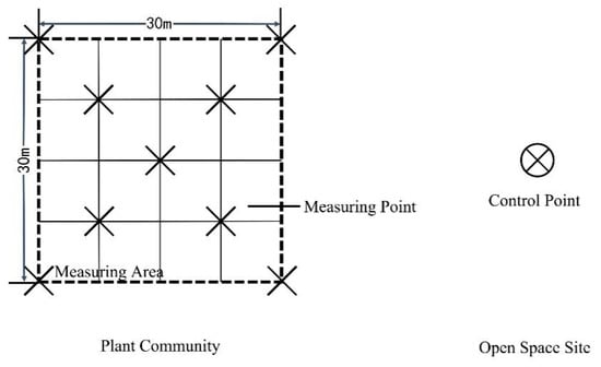
Figure 5.
Schematic diagram of measuring and control point allocation in the trial site.
2.2. Data Source
2.2.1. Time and Index of Measurement
To reduce the error caused by weather, we selected a typical sunny, hot summer afternoon (with no wind or only breeze, the highest temperature reached 41 °C). The study period was from 30 July 2016 to 5 August 2016. Within the regular sight-seeing time (8:00 AM–18:00 PM), measurements were conducted every two hours. A total of 315 groups of sample data were obtained. The indices of measurement included DBH (diameter at breast height), crown breadth, canopy density, porosity, temperature, and relative humidity. We defined the cooling and humidifying effects into the temperature difference and cooling rate, and relative humidity difference and humidification rate, respectively. The specific Equations (1)–(4) are as follows
where dTdiff (°C) is the temperature difference; T is the temperature of the test point; T0 is the temperature of the control point; dRHdiff (%) is the relative humidity difference; RH is the relative humidity of the test point; RH0 is the relative humidity of the control point; dTratio (%) is the cooling rate; and dRHratio (%) is the humidification rate.
dTdiff (°C) = T − T0
dRHdiff (%) = RH − RH0
dTratio (%) = (T0 − T)/T0
dRHratio (% )= (RH − RH0)/RH0
2.2.2. Measurement Methods
An NK4000 (Kestrel 4000, Boothwyn, Pennsylvania, PA, USA) portable weather station [37] was applied to measure the temperature and relative humidity of samples, with a measuring height of 1.5 m (the height at which humans are most sensitive to environmental factors). Every sample was measured three times at each test time, where the used measurement value was the average of the three values. The data of the average of DBH, crown breadth, tree height, and clear bole height were recorded at the sample spot, in order to understand the community structure and the associated indices.
Canopy density is the ratio of the sky sphere which is covered by the branches of trees when looking up at a given point in a woodland [38]. Porosity is the ratio of the projected area of transparent pores on the vertical plane of the forest edge to the total projected area of the forest belt on the vertical plane [39]. Canopy density and porosity were mainly measured by digital image processing. Single vegetation instances had relatively large area and different degrees of porosity at different positions. To better record the environmental difference at each experimental point, a Canon 650D camera (Canon, Tokyo, Japan) was applied to take photos of the vertical images. The porosity could be generated by calculating the ratio of the projected area of the transparent pores on the vertical plane of the image to the total projected area of the edge of the forest belt. The camera was maintained in a horizontal orientation 1.5 m from the ground and a fish-eye lens was attached to it, in order to take photos of the canopy (from underneath) at the nine measuring points of each community. The obtained hemispherical canopy digital images were processed and analyzed using the Adobe Photoshop CS6 software (Adobe Photoshop 13.0), thereby generating the canopy density of each sample [40,41]. The general situation of the communities is given in Table 1.

Table 1.
Survey of different vegetation types of trial site.
2.3. Dummy Variable Regression Model
The major factors that influence plant communities, in terms of relieving the heat island effect, include canopy density, porosity, vegetation types, etc. While these feature parameters have mutual effects, a traditional single scatter plot cannot comprehensively demonstrate the mutual effects of these variables. Therefore, the dummy variable model was employed in this paper, where we mainly used the function of describing the interactions among attribute variables [42,43]. A dummy variable, in essence, cannot be counted as a type of variable (e.g., a continuous or categorical variable). The dummy variable technology is used to transform polytomous variables into binary variables. After virtualization, this variable is regarded as an explanatory variable and applied in a regression model [44]. The advantage of this method is that multiple factors are included in the whole sample, which enlarges the sample size and reduces the experimental error.
We first quantified dummy variables (density, porosity, and vegetation types), constructed a segmented regression model, and built regression equations of temperature and humidity, respectively, using the structural parameters and vegetation types of the two communities. Then, a table of regression model results was generated for each measuring index, based on the associated dummy variable, in order to discern the optimal structural parameter range of communities that could perform different ecological functions.
According to the language of dummy variables, the average cooling and humidifying volume were defined as y, and the coupling regression equation of the performance value of each ecological function (i.e., cooling and humidifying volume) and the three independent variables could be built, accordingly. The Equation (5) is
where ai, bj, and ck are the coefficients of the independent variables vcdi, vpj, and typek, respectively, and vcd1, vp1, and type1 were set as control groups within the experimental points. As all dummy variables in the first group were valued 0, constant terms were regarded as the average of the first group.
Nine points were evenly and respectively selected in the nine chosen single-plant communities (selection method is shown in Figure 5). The canopy densities and porosities at these points varied. Part of the dummy variable model process involves dividing the independent variables into dummy variables, which is also convenient for finding their thresholds. The data generated at all trial points were classified into the following ranges (namely, dummy variables):
- (1)
- VCD: The measured concentration range of vcd was 0.60–0.95. This variable is an ordered categorical variable. Therefore, six dummy variables could be generated after quantification: vcd2 (canopy density 0.65–0.70), vcd3 (canopy density 0.71–0.75), vcd4 (canopy density 0.76–0.80), vcd5 (canopy density 0.81–0.85), vcd6 (canopy density 0.86–0.90), and vcd7 (canopy density 0.91–0.95);
- (2)
- VP: The measured concentration range of vp was 0.15–0.60. This variable is an ordered categorical variable. Therefore, six dummy variables could be generated after quantification: vp2 (porosity 0.26–0.30), vp3 (porosity 0.31–0.35), vp4 (porosity 0.36–0.40), vp5 (porosity 0.41–0.45), vp6 (porosity 0.46–0.50), and vp7 (porosity 0.51–0.60);
- (3)
- Type: There were nine types of plant in the trial site. This variable is an unordered variable that was equally distributed. Therefore, eight dummy variables could be generated after quantification: type2 (Cerasus), type3 (Acer palmatum), type4 (Liquidambar formosana), type5 (Sapium sebiferum), type6 (Osmanthus fragrans), type7 (Cercis chinensis), type8 (Cinnamomum camphora), and type9 (Atropurpureum).
3. Results
3.1. Regression Equation of Cooling Volume and Relevance Test
The cooling volume passed the F-test at the significance level of 1%. The regression results showed a highly significant difference (p < 0.01); while R2 = 0.88, demonstrating a relatively good whole regression fit.
Table 2 shows that the coefficients of canopy density were all significantly positive, demonstrating a positive relationship with cooling volume. The coefficients exhibited an increasing trend, indicating that an increase in canopy density may partially increase the positive influence on cooling volume. Canopy density exhibited a highly significant difference at the level of 1%, demonstrating that, along with the increase in canopy density (within a certain range), the temperature of vegetation communities and control bare ground had a larger difference, and the communities had a lower daily temperature and better cooling effect. All coefficients of porosity were positive, reflecting the positive influence of porosity on cooling volume. It exhibited a significant difference at the 10% level in the range of 0.26–0.35 and a highly significant difference in the range of 0.46–0.50, suggesting the largest impact on cooling effect in this range. The vegetation of L. formosana and C. chinensis had insignificant differences from M. grandiflora (the coefficient of Magnolia grandiflora was regarded as 0.000), while the cooling effects of Cerasus, A. palmatum, C. camphora, and Atropurpureum had highly significant differences (Figure 6).
Table 2.
Regression analysis on canopy density, porosity, vegetation types and cooling volume.
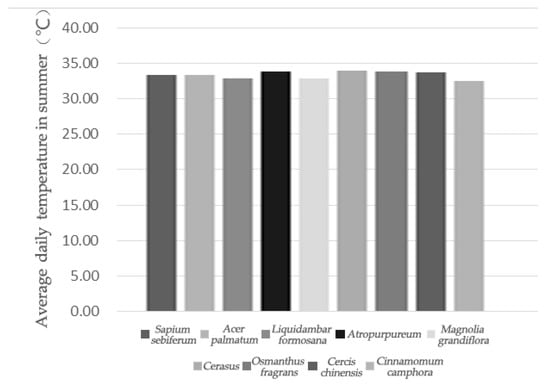
Figure 6.
Average daily temperature per unit green area of different pure forests in summer.
3.2. Regression Equation of Humidifying Volume and Relevance Test
Humidifying volume passed the F-test at a significance level of 1%, reaching a highly significant difference (p < 0.01); while R2 = 0.84, demonstrating a relatively good whole regression fit. Table 3 shows that the coefficient of the canopy density variable was positive, showing a positive relationship with humidifying volume, presenting significant relevance. The coefficient of the porosity variable was negative, showing a negative relationship with humidifying volume. This indicates that, in a certain range, the higher the porosity ratio of the community cross-section, the better the air circulation, thus leading to a worse humidifying effect; however, this exhibited relatively low significance. The p-value distribution of the vegetation type dummy variable in Table 3 indicates that the humidifying effects of O. fragrans, C. camphora, and Atropurpureum vegetation had no significant differences from M. grandiflora vegetation (the coefficient of M. grandiflora was regarded as 0.000). The average daily humidity capacity of each tree species is shown in Figure 7.
Table 3.
Regression analysis on canopy density, porosity, vegetation type, and humidifying volume.
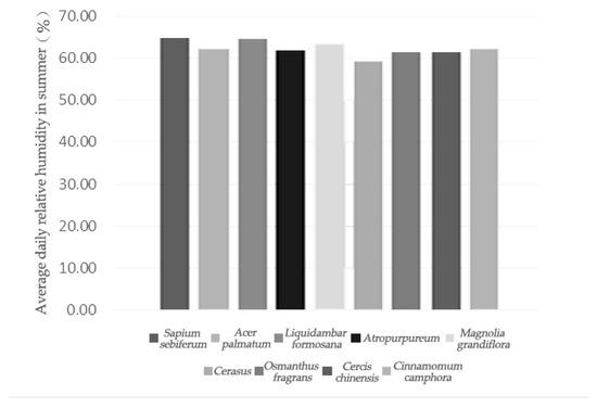
Figure 7.
Average daily humidity per unit green area of different pure forests in summer.
3.3. Average Analysis of Regression Model Based on Dummy Variables
Canopy density and porosity are common parameters for describing plant communities. In order to further examine the specific influence of different vegetation types on cooling and humidifying effects, as well as to figure out the optimal ranges of canopy density and porosity for vegetation, we compared the mean values of the two variable regression models.
3.3.1. Mean Value of Regression Model of Canopy Density, Porosity, and Cooling Volume
Table 4 shows that, for one range of porosity—apart from individual values—the increase in canopy density followed a general increasing trend of cooling volume, where the total cooling volume for relatively low canopy density was significantly lower than that for relatively high canopy density.
Table 4.
Mean values of the regression model of canopy density, porosity, and cooling volume.
Table 4 also demonstrates that, when the canopy density was higher than 0.9, the cooling volume exhibited a decreasing trend. This result indicates that, based on the influence of the outer environment and the growth features of vegetation, for communities within a certain measurement range, the higher canopy density of vegetation led to a higher cooling effect. However, overcrowded vegetation prevented air diffusion and circulation, thereby negatively influencing the cooling effect. In order to maintain the cooling volume at a relatively high level, the optimal range of canopy density was determined as 0.81–0.85, while the optimal range of porosity was 0.31–0.35.
3.3.2. Mean Value Results of Regression Model of Canopy Density, Porosity, and Humidifying Volume
Table 5 shows that, for one range of porosity—apart from individual values—the increase in canopy density followed a significantly increasing trend for humidifying volume, presenting a significant positive relationship with canopy density. The general humidifying volume at relatively low porosity was higher than that for relatively low porosity, exhibiting a certain negative influence on the humidifying effect. Therefore, to maintain humidifying volume at a relatively high level, the optimal range of canopy density was 0.81–0.85, while that of porosity was 0.31–0.35.
Table 5.
Mean values of regression model of canopy density, porosity, and humidifying volume.
3.3.3. Analysis on Threshold of Community Structure Parameters of the Aggregated Green Infrastructure
According to the above analyses, the optimal range of canopy density was 0.81–0.85, while that of porosity was 0.31–0.35, in order to keep the cooling and humidifying effects at relatively high levels. These results demonstrate that the urban aggregated green infrastructure can facilitate cooling and humidifying effects, which may serve to alleviate the urban heat island effect. Plant communities with high density and a complex structure had better cooling and humidifying effects. However, very high canopy density and very low porosity were not conducive to air circulation in the community, and so the heat emission was slow, resulting in a poor cooling effect for plants and no obvious humidifying effect. Therefore, the best cooling and humidifying effects of plant communities were obtained with the range of canopy density being 0.81–0.85 and that of porosity being 0.31–0.35.
4. Discussion
4.1. The Dummy Variable Method
At present, most experimental data—with respect to the cooling and humidifying of urban aggregated green infrastructure—were obtained by actual measurement or remote sensing. There may be experimental errors in the data acquisition or analysis, due to other factors that could not be adjusted. Thus, it is important to consider the impact of any potential confounding variables which may bias the estimate of the cooling effect of a green space. In this study, we attempted to solve the problem of determining the quantitative relationships of community parameters; therefore, we introduced the dummy variable model to define the optimal threshold, such that the abnormal factors were included in the overall sample, the data sample size was expanded, and the experimental error was reduced [45]. The application of virtual variable regression analysis in the relevant literature has mainly focused on natural plant communities and urban meteorological monitoring points [46,47,48]; for instance, virtual variables were used to analyze the dynamic effects of the Urban Haze control program [49], build single-tree biomass models [50,51], and to identify the differences in spectral response between two types of forest disturbances and their temporal dynamics [52]. As a typical urban aggregated green infrastructure plant community has a relatively small area, real-time monitoring at allocated points can be applied for data acquisition. In addition, due to the complicated surroundings and various vegetation types inherent in urban aggregated green infrastructure, the key advantage of using dummy variables is in reducing the interference of outer influence factors, in order to effectively classify and analyze the variables in the experiment. Therefore, the dummy variable regression analysis herein can be taken as a reference for future interdisciplinary ecological research.
4.2. Threshold Value of Plant Community Structure Parameters in the Aggregated Green Infrastructure
Many studies have shown that trees can affect the air temperature and relative humidity through shading, transpiration, and evaporative cooling. There has been some evidence that the cooling effect of a plant community increased with its canopy density, although it was not clear whether there was a better threshold or if there is a simple linear relationship. Our study results showed that the canopy density of urban aggregated green infrastructure had a significant positive correlation with cooling and humidifying, while the porosity had a positive correlation with cooling but a negative correlation with humidifying effect, respectively. These findings were similar to previous research results [18,53]. At present, most studies have focused on the correlations between canopy density, porosity, and cooling and humidifying, while few have paid attention to parameter thresholds [54,55]. Zhu reported that, when the canopy density reached 44%, the effect became significant. When the canopy density exceeded 67%, the effect was significant and stable [56]. In this paper, we further discussed the threshold values optimizing the effects of canopy density and porosity on the mitigation of heat island effect. By introducing dummy variables, the two community structure parameters—namely, porosity and canopy density—could be introduced into the model. Our results suggest that, when the canopy density is 0.81–0.85 and the porosity is 0.31–0.35, the effects of community cooling and humidifying are optimal. In conclusion, due to different performances in alleviating the heat island effect, as well as the different canopy densities and porosities of different communities, a comprehensive choice considering factors such as regional features, growing situations, community structure, and vegetation types could lead to a reasonable allocation of vegetation, in order to reduce the urban heat island effect and, further, reduce the influence of hot weather on the natural and living environment.
4.3. Effects of Plant Community Structure Parameters on Cooling and Humidifying in Aggregated Green Infrastructure
Previous studies on urban green infrastructure have mostly focused on the community complex [57,58,59]. Zhang et al. studied the cooling and humidifying effects of vegetation communities in Shanghai, and found that communities with more complicated structure, high canopy closure, large leaf area index, and high plant height had more significant cooling and humidifying effects [60]. Few detailed attempts have been made to directly understand the correlations between cooling and humidifying effects and urban aggregated green infrastructure. In this study, we assessed the urban aggregated green infrastructure, where our related results confirm previous studies. Previous studies in Beijing [17], Shenzhen [61], Osaka [62], and London [63] have concluded that the leaf area and canopy density indices have significant relevance for cooling and humidifying effects. Some studies have shown that aggregated green infrastructure with more than 50% hard cover and almost no arbor and shrub coverage may not have obvious cooling and/or humidifying effects. Therefore, canopy density is particularly important for promoting cooling and humidifying effects. In the aggregated green infrastructure, the overall greening coverage rate is usually more than 60% [6]. In this study, canopy density had a significant positive influence on both cooling and humidifying effects, while porosity had positive relevance to the cooling effect and negative relevance to the humidifying effect. This pattern may have been due to the cross-section of summer community having high porosity and good breathability, which is good for air circulation, thereby leading to a rapid decrease inf temperature. Outer air comes into the humid inner space and takes vapor away, thereby reducing the relative humidity of the community. Therefore, it is equally important to increase the complexity of the spatial types in aggregated green infrastructure [64]. Having a certain area or proportion of open space and water is conducive to the circulation of air, reducing the environmental temperature and achieving the purpose of collaborative cooling. As for future research, there is a strong need for multi-scale studies combining actual measurements with remote sensing, in order to improve the accuracy. Therefore, we suggest that a key line of future research is to explicitly investigate the distance- and size-dependence of the effects of green areas, allowing explicit bottom-up predictions of the effects of particular amounts and spatial arrangements of greening.
5. Conclusions
We applied a virtual variable regression model, reduced the mutual effect of various factors, and quantized the relationship equations of structural parameters of community parameters and vegetation types with cooling and humidifying effects. We also applied mean value tables, in order to determine the optimal ranges of canopy density and porosity, thus providing quantitative models for an efficiency evaluation system regarding alleviating the heat island effect by means of urban aggregated green infrastructure.
We showed that canopy density had significantly positive relationships with both cooling and humidifying effects, while porosity had a positive relationship with the cooling effect and a negative relationship with the humidifying effect. Different types of vegetation had different influences on cooling and humidifying effects. The cooling and humidifying effects of vegetation communities were optimal when the canopy density was in the range of 0.81–0.85 and the porosity was in the range of 0.31–0.35. This paper initially summarizes three characteristics which are key for urban aggregated green infrastructure: that the area is larger than three hectares, the spatial types should be diverse and complex, and the greening coverage rate should be more than 60%. This study provides a better understanding of how to handle the heat island effect, thereby improving human well-being.
Author Contributions
Conceptualization, J.W.; methodology, J.W. and Y.W.; software, H.L.; validation, J.W. and Y.W.; formal analysis, H.L.; investigation, J.W. and X.X.; resources, J.W.; data curation, H.L.; writing—original draft preparation, J.W.; writing—review and editing, H.L.; visualization, H.L.; supervision, J.W., X.X. and Y.W.; project administration, J.W., X.X. and Y.W.; funding acquisition, J.W. and Y.W. All authors have read and agreed to the published version of the manuscript.
Funding
This study supported by Shanghai Committee of Science & Technology Fund (No. 19DZ1203303) and National Natural Science Foundation of China (No.51978479), and supported by Jiangsu Committee of Science & Technology Fund (No. SBK2019044048) and National Natural Science Foundation of China (No.32001360).
Conflicts of Interest
The authors declare no conflict of interest.
References
- Lionel, S.V.; Madhumitha, J.; Harini, N. Effect of street trees on microclimate and air pollution in a tropical city. Urban For. Urban Green. 2013, 12, 408–415. [Google Scholar]
- Barbieri, T.; Despini, F.; Teggi, S. A multi-temporal analyses of land surface temperature using landsat-8 data and open source software: The case study of Modena. Sustainability 2018, 10, 1678. [Google Scholar] [CrossRef]
- Ariane, M.; Kathrin, H.; Anthony, J.B. Impact of urban form and design on mid-afternoon microclimate in Phoenix Local Climate Zones. Landsc. Urban Plan. 2014, 122, 16–28. [Google Scholar]
- Amani-Beni, M.; Zhang, B.; Xie, G.; Xu, J. Impact of urban park’s tree, grass and water body on microclimate in hot summer days: A case study of Olympic Park in Beijing, China. Urban For. Urban Green. 2018, 32, 1–6. [Google Scholar] [CrossRef]
- Richard, T.F. Some general principles of landscape and regional ecology. Landsc. Ecol. 1995, 10, 133–142. [Google Scholar]
- Cao, X.; Onishi, A.; Chen, J.; Imura, H. Quantifying the cool island intensity of urban parks using ASTER and IKONOS data. Landsc. Urban Plan. 2010, 96, 224–231. [Google Scholar] [CrossRef]
- Chang, C.R.; Li, M.H.; Chang, S.D. A preliminary study on the local cool-island intensity of Taipei city parks. Landsc. Urban Plan. 2007, 80, 386–395. [Google Scholar] [CrossRef]
- Wu, F.; Li, S.H.; Liu, J.M. Research on the relationship between urban green spaces of different areas and the temperature and humidity benefit. Chin. Landsc. Architect. 2007, 27, 71–74. [Google Scholar]
- Gudina, L.F.; Klaus, D.; Henrik, M. Efficiency of parks in mitigating urban heat island effect: An example from Addis Ababa. Landsc. Urban Plan. 2014, 123, 87–95. [Google Scholar]
- Zhang, B.; Xie, G.D.; Gao, G.X.; Yang, Y. The Cooling Effect of Urban Green Spaces As a study in Beijing, China. Build. Environ. 2014, 76, 37–43. [Google Scholar] [CrossRef]
- Jim, C.Y.; Chen, W.Y. Assessing the Ecosystem Service of Air Pollutant Removal by Urban Trees in Guangzhou (China). J. Environ. Manag. 2008, 88, 665–676. [Google Scholar] [CrossRef] [PubMed]
- Chen, L.; Xie, G.D.; Gai, L.Q.; Pei, S.; Zhang, C.-S.; Zhang, B.; Xiao, Y. Research on Noise Reduction Service of Road Green Spaces—A Case Study of Beijing. J. Nat. Resour. 2011, 26, 1526–1534. [Google Scholar]
- Xia, B.; Zhang, B.; Xie, G.D.; Zhang, C.Q. The Value-Added Effect of Park Green Space on Residential Property in Beijing. Resour. Sci. 2012, 34, 1347–1353. [Google Scholar]
- Gao, J.X.; Song, T.; Zhang, B.; Han, Y.W.; Gao, X.T.; Feng, C.Y. The Relationship Between Urban Green Space Community Structure and Air Temperature Reduction and Humidity Increase in Beijing. Resour. Sci. 2016, 38, 1028–1038. [Google Scholar]
- Gao, K.; Qin, J.; Song, K.; Hu, Y. Fallen Temperature Effects at Green Patches of Urban Residential Areas and Analysis of Its Influence Factors. J. Plant Resour. Environ. 2009, 18, 50–55. [Google Scholar]
- Li, Z.D.; Qin, Z. Influence of canopy structural characteristics on cooling and humidifying effects of Populus tomentosa community on calm sunny summer days. Landsc. Urban Plan. 2014, 127, 75–82. [Google Scholar]
- Han, H.J.; Zhou, Y.W. Cooling and Moisturizing Effect of Different Afforested Tree Species in July. J. Hebei Agric. Sci. 2007, 5, 28–30. [Google Scholar]
- Liu, J.M.; Li, S.H.; Yang, Z.F. Temperature and Humidity Effect of Urban Green Spaces in Beijing in Summer. Chin. J. Ecol. 2008, 27, 1972–1978. [Google Scholar]
- Qin, Z.; Li, Z.D. Impact of canopy structural characteristics on inner air temperature and relative humidity of Koelreuteria paniculata community in summer. Chin. J. Appl. Ecol. 2015, 26, 1634–1640. [Google Scholar]
- Leuning, R.; Hughes, D. A Multi-Angle Spectrometer for Automatic Measurement of Plant Canopy Reflectance Spectra. Remote Sens. Environ. 2015, 103, 236–245. [Google Scholar] [CrossRef]
- Kermavnar, J.; Marinsek, A. Evaluating Short-Term Impacts of Forest Management and Microsite Conditions on Understory Vegetation in Temperate Fir-Beech Forests: Floristic, Ecological, and Trait-Based Perspective. Forests 2019, 10, 909. [Google Scholar] [CrossRef]
- Aude, E.; Lawesson, J.E. Vegetation in Danish Beech Forests: The Importance of Soil, Microclimate and Management Factors, Evaluated by Variation Partitioning. Plant Ecol. 1998, 134, 53–65. [Google Scholar] [CrossRef]
- Sun, C.H.; Su, Y.X.; Han, L.S.; Wu, J.P.; Liu, L.Y.; Chen, X.Z.; Deng, Y.J.; Yang, H.Z.; Jiang, J.; Lin, H. The Simulation and Spatial-temporal variations of Atmospheric Rainfall Interception by Vegetation Canopies Based on MODIS LAI Data at the Basin Scale in the Guangdong Province from 2004 to 2016. Acta Ecol. Sin. 2020, 4040, 2252–2266. [Google Scholar]
- Bian, H.J.; Fu, H.M. Effects of Tree Canopy on the Concentration and Dry Deposition Velocity of Particles in Outdoors. J. Donghua Univ. Nat. Sci. 2019, 45, 924–937. [Google Scholar]
- Navarret, H.P.; Laffan, K. A Greener Urban Environment: Designing Green Infrastructure Interventions to Promote Citizens’ Subjective Well-Being. Landsc. Urban Plan. 2019, 109, 103618. [Google Scholar] [CrossRef]
- Aram, F.; Solgi, E. The Cooling Effect of Large-Scale Urban Parks on Surrounding Area Thermal Comfort. Energies 2019, 12, 3904. [Google Scholar] [CrossRef]
- Buijs, A.; Hansen, R. Mosaic Governance for Urban Green Infrastructure: Upscaling Active Citizenship from a Local Government Perspective. Urban For. Urban Green. 2019, 40, 53–62. [Google Scholar] [CrossRef]
- Sasaki, T.; Ishii, H. Evaluating Restoration Success of a 40-year-old Urban Forest in Reference to Mature Natural Forest. Urban For. Urban Green. 2018, 32, 123–132. [Google Scholar] [CrossRef]
- Qin, Z. Cooling and Humidifying Effects and Driving Mechanisms of Beijing Olympic Forest Park in Summer. Ph.D. Thesis, Beijing Forestry University, Beijing, China, 2016. [Google Scholar]
- Jansson, C.; Jansson, P.E.; Gustafsson, D. Near surface climate in an urban vegetated park and its surroundings. Theor. Appl. Climatol. 2007, 89, 185–193. [Google Scholar] [CrossRef]
- Chow, W.T.L.; Pope, R.L.; Martin, C.A.; Brazel, A.J. Observing and modeling the nocturnal park cool island of an arid city:Horizontal and vertical impacts. Theor. Appl. Climatol. 2011, 103, 197–211. [Google Scholar] [CrossRef]
- Yu, Z.W.; Yang, G.Y.; Jørgensen, G. Critical review on the cooling effect of urban blue-green space: A threshold-size perspective. Urban For. Urban Green. 2020, 49, 126630. [Google Scholar] [CrossRef]
- Sha, X.M. Effects of Seasonal Changes of Garden Plants on the Construction of Spatial Landscape Pattern. Mol. Plant Breed. 2018, 16, 3078–3084. [Google Scholar]
- Zhang, Z.J.; Zhang, Y.F.; Jin, L. Thermal comfort in interior and semi-open spaces of rural folk houses in hot-humid areas. Build. Environ. 2018, 128, 336–347. [Google Scholar] [CrossRef]
- Skoulika, F.; Santamouris, M.; Kolokotsa, D.; Boemi, N. On the thermal characteristics and the mitigation potential of a medium size urban park in Athens, Greece. Landsc. Urban Plan. 2014, 123, 73–86. [Google Scholar] [CrossRef]
- Jaganmohan, M.; Knapp, S.; Buchmann, C.M.; Schwarz, N. The bigger, the better? The influence of urban green space design on cooling effects for residential areas. J. Environ. Qual. 2016, 45, 134. [Google Scholar] [CrossRef]
- Zheng, J.J.; Zhang, J.L. Calculation on Microclimate Benefits Urban Green Space in Huanggang City. Hubei For. Sci. Technol. 2010, 3, 6–9. [Google Scholar]
- Wang, X.S.; Teng, M.J.; Zhou, Z.X. Canopy density effects on particulate matter attenuation coefficients in street canyons during summer in the Wuhan metropolitan area. Atmos. Environ. 2020, 240, 117739. [Google Scholar] [CrossRef]
- Zhu, J.J.; Matsuzaki, T.; Gonda, Y. Optical stratification porosity as a measure of vertical canopy structure in a Japanese coastal forest. For. Ecol. Manag. 2003, 173, 89–104. [Google Scholar] [CrossRef]
- Kong, F.; Yan, W.; Zheng, G.; Yin, H.; Cavan, G.; Zhan, W.; Zhang, N.; Cheng, L. Retrieval of three-dimensional tree canopy and shade using terrestrial laser scanning (TLS) data to analyze the cooling effect of vegetation. Agric. For. Meteorol. 2016, 217, 22–34. [Google Scholar] [CrossRef]
- Liu, X.H. Influence of Plantation Ecosystems on Atmospheric Particles Concentration in Beijing Region. Ph.D. Thesis, Beijing Forestry University, Beijing, China, 2016. [Google Scholar]
- Roh, H.J. Developing Cold Region Winter Weather Traffic Models and Testing Their Temporal Transferability and Model Specification. J. Cold Regions Eng. 2019, 33. [Google Scholar] [CrossRef]
- Xu, J.M. Study on Evaluation and Sustainable Utilization of the Wetlands in Yellow River Delta (Dongying). Ph.D. Thesis, Chinese Academy of Agricultural Sciences (CAAS), Beijing, China, 2001. [Google Scholar]
- Cao, Y.R. Analysis and Implementation of Virtual Variable Regression in SPSS. Stat. Decis. 2018, 34, 66–69. [Google Scholar]
- Mihai, F.V.; Philip, G.C. Microclimatic and spruce growth gradients adjacent to young aspen stands. For. Ecol. Manag. 2006, 221, 13–26. [Google Scholar]
- Tao, W.G.; Xu, B.; Liu, L.J.; Yabg, X.-C.; Qin, Z.-H. Yield Estimation Model for Different Utilization Status Grassland Based on Remote Sensing Data. Chin. J. Ecol. 2007, 3, 332–337. [Google Scholar]
- Xie, X.Q.; Xu, Y. Comprehensive Prediction about PM2.5 Concentrations in the Atmosphere. Electr. Power Technol. Environ. Protect. 2015, 2, 1–4. [Google Scholar]
- Liu, H.X.; Lu, Z.Y.; Jin, G.X.; Sun, G.P.; Wu, J.; Xu, L.J.; Xu, C.Y. The Influence of Canopy Structure on Comfort and Microclimate in Urban Forest in Summer in Beijing. J. Fujian Agric. For. Univ. Nat. Sci. Ed. 2018, 47, 736–742. [Google Scholar]
- Mao, X.Q.; Zhang, Q.Y. Evaluation of the effectiveness of “2 + 26” Cities’Haze Control Scheme: A case study of Shandong Province. China Popul. Resour. Environ. 2020, 30, 83–92. [Google Scholar]
- Shen, J.P.; Chen, D.S.; Sun, X.M. Modeling a single-tree biomass equation by seemingly unrelated regression and dummy variables with Larix kaempferi. J. Zhejiang A F Univ. 2019, 36, 877–885. [Google Scholar]
- Jin, J.; Wang, Q. Evaluation of Informative Bands Used in Different PLS Regressions for Estimating Leaf Biochemical Contents from Hyperspectral Reflectance. Remote Sens. 2019, 11, 197. [Google Scholar] [CrossRef]
- Martin, H.; Magda, J.; Jakub, L. Comparison of two types of forest disturbance using multitemporal Landsat TM/ETM+ imagery and field vegetation data. Remote Sens. Environ. 2009, 113, 835–845. [Google Scholar]
- Qin, Z.; Ba, C.B.; Li, Z.D. Effects of Different Plant Communities on Temperature Reduction and Humidity Increase in Beijing. Ecol. Sci. 2012, 5, 567–571. [Google Scholar]
- Emily, B.P.; McFadden, J.P. Influence of seasonality and vegetation type on suburban microclimates. Urban Ecosyst. 2010, 13, 443–460. [Google Scholar]
- Zhu, C.Y.; Ji, P.; Li, S.H. Effects of the Different Structure of Urban Green Belts on the Air Quality. J. Nanjing For. Univ. Nat. Sci. Ed. 2013, 1, 18–24. [Google Scholar]
- Zhu, C.Y.; Li, S.H.; Ji, P. Relationships between urban green belt structure and temperature-humidity effect. Chin. J. Appl. Ecol. 2011, 22, 1255–1260. [Google Scholar]
- Kabila, A.; Divine, O.A.; Kwadwo, A. Does green space matter? Public knowledge and attitude towards urban greenery in Ghana. Urban For. Urban Green. 2019, 46, 126462. [Google Scholar]
- Sarah, L.; Stephan, P.; Kumelachew, Y. Rethinking urban green infrastructure and ecosystem services from the perspective of sub-Saharan African cities. Landsc. Urban Plan. 2018, 180, 328–338. [Google Scholar]
- Bertrand, F.N.; Daniel, C.; Alexander, A.; Manfred, D. Urban Green Spaces Enhance Climate Change Mitigation in Cities of the Global South: The Case of Kumasi, Ghana. Procedia Eng. 2017, 198, 69–83. [Google Scholar]
- Zhang, M.L.; Qin, J.; Hu, Y.H. Effects of Temperature Reduction and Humidity Increase of Plant Communities in Shanghai. J. Beijing For. Univ. 2008, 2, 39–43. [Google Scholar]
- Zhang, Z.; Lv, Y.M.; Pan, H.T. Cooling and humidifying effect of plant communities in subtropical urban parks. Urban For. Urban Green. 2013, 12, 323–329. [Google Scholar] [CrossRef]
- Yuan, J.H.; Kazuo, E.; Craig, F. Is urban albedo or urban green covering more effective for urban microclimate improvement?: A simulation for Osaka. Sustain. Cities Soc. 2017, 32, 78–86. [Google Scholar] [CrossRef]
- Joseph, L.M.; Kieron, J.D.; Stefan, S. Influence of evaporative cooling by urban forests on cooling demand in cities. Urban For. Urban Green. 2019, 37, 65–73. [Google Scholar]
- Shashua-Bar, L.; Hoffman, M.E. Quantitative evaluation of passive cooling of the UCL microclimate in hot regions in summer, case study: Urban streets and courtyards with trees. Build. Environ. 2004, 39, 1087–1099. [Google Scholar] [CrossRef]
Publisher’s Note: MDPI stays neutral with regard to jurisdictional claims in published maps and institutional affiliations. |
© 2021 by the authors. Licensee MDPI, Basel, Switzerland. This article is an open access article distributed under the terms and conditions of the Creative Commons Attribution (CC BY) license (http://creativecommons.org/licenses/by/4.0/).