Statistical Unfolding Approach to Understand Influencing Factors for Taxol Content Variation in High Altitude Himalayan Region

Abstract

Taxol drugs can be extracted from various species of the taxaceae family. It is an alkaloid (metabolic product) used for the treatment of various types of cancer. Since taxol is a metabolic product, multiple aspects such as edaphic, biochemical, topographic factors need to be assessed in determining the variation in Taxol Content (TC). In this study, both sensor-based hyperspectral reflectance data and absorption-based indices were tested together for the development of an advanced statistical unfolding approach to understand the influencing factors for TC in high altitude Himalayan region. Seriation analysis based on permutation matrix was applied with complete linkage and a multi-fragment heuristic scaling rule along with the common techniques such as Principal Component Analysis (PCA) and correlation to understand the relationship of TC with various factors. This study also tested the newly developed taxol indices to rule out the possibility of overlapping of TC determining bands with the foliar pigment’s wavelengths in the visible region. The result implies that T. wallichiana with a high TC is found more in its natural habitat of deep forest, relating it indirectly to elevation in the case of the montane ecosystem. Taxol is the most varying parameter among the measured variables, followed by hyperspectral Taxol content (TC) indices such as TC 2, TC 5, and carotenoids, which suggests that the indices are well versed to capture variations in TC with elevation.

1. Introduction

Recent studies have shown that the turnover in tree species composition across edaphic and elevational gradients can be strongly correlated with the functional traits [1]. These factors affect plant growth via various means and can be used to characterize different ecosystems. The major determining components of vegetation include biochemical constituents that are central to their physiological form and function, along with water, chlorophyll, and accessory pigments, nitrogen, cellulose, starch, sugars, lignin, and protein. These are the mandatory parameters for describing the nutritional status of any tree of a particular ecosystem [2,3], while the secondary metabolites such as terpenes, sesquiterpenes, phytosterols, etc., are more useful to humans [4], which makes the plant economically valuable.

The majority of studies have been carried out to acknowledge and retrieve these determining variables and the effects on vegetation using various models and remote sensing techniques, but the relative effects of all these factors have not been addressed intricately with proper research findings [5]. The spatial and temporal variation of these properties offers great help in understanding and evaluating physiological conditions such as photosynthesis, evapotranspiration, secondary metabolites formation, and deriving plans for the conservation of the ecosystem [2,6]. Now, researchers are focusing on covariation trait studies to determine definite functional indicators for ecological and biodiversity conservation [7,8].

Taxus wallichiana Zucc. is a tree species that belongs to the family Taxaceae and is popularly known as the Himalayan yew, which is globally distributed in Europe, North America, North India, Pakistan, China, and Japan. In Asia, its variation and availability extend from Afghanistan through the great Himalayas to the Philippines, and it is widely distributed in countries such as Pakistan and India. Recently, it gained widespread attention on a global scale because its leaves and bark were found to be rich in taxol, which is a potential anti-cancerous drug [9]. Taxol is known to have first been isolated from the bark of Taxus brevifolia, and since then, taxol and related bioactive taxoids have been reportedly found in the various other species of the same genus Taxus. Due to the overexploitation of this group of species, it is currently endangered as per IUCN and on the verge of extinction. Moreover, several species are disappearing at an alarming rate mainly at higher altitudes due to over-harvesting, habitat destruction, and abrupt climate change [10,11]. Altitudinal variation influences the ecological factors and, thus, the ecosystem. Factors including soil nutrients, precipitation, and mean temperature directly or indirectly affect the secondary metabolite amount and biological activities of the plants [7].

The extraction and estimation of secondary metabolites such as TC are always expensive, time-consuming, and tedious. The non-destructive method of taxol estimation for conservation and planning becomes vital. A few researchers such as Kokaly et al. [1] have characterized the plant phenolics (another secondary metabolite) [12] to their hyperspectral signature at a 1660-nanometer wavelength. Phenolics are characterized using continuum removal, which is a technique used to isolate and analyze the features in reflectance spectra acquired using hyperspectral sensors. Hyperspectral remote sensing (HSR) is a new dimension of remote sensing with a higher number of band data in a continuous form that gives fine resolution to obtain detailed information on the object [13]. Many scientists have characterized different species in the same area using HSR [14]. Keystone species conservation is the next logical step that can be brought by HSR [15]. ‘Curse of dimensionality’ is the phrase used for high dimensional hyperspectral data. This problem can be remedied by indices used for the retrieval of a particular parameter. These indices are easy to use and require less time and a less sophisticated system to compute [16].

The canopy confounding variables such as foliar nitrogen, chlorophyll, cellulose, etc., are successfully estimated using vegetation indices when applied to remote sensing data. The spectral wavelengths region near 550 and 700 nm, as well as the red-edge region (680–780 nm), have been utilized for assessing chlorophyll by many researchers in hyperspectral remote sensing [17,18,19]. Wang et al. [20] estimated nitrogen accurately in cases of broadleaf, needle leaf, and mixed forests plots using Normalized Difference Nitrogen Index (NDNI) centered at 1510 nm. However, an indirect relationship occurs between nitrogen and chlorophyll that generates a correlation between Near InfraRed (NIR) reflectance (800–850 nm) and canopy foliar mass-based nitrogen concentration [21]. Similarly, reflectance in the visible wavelengths 400–700 nm is dominated by absorptions from foliar pigments [22]. Among the pigments, chlorophyll a and b have the strongest effect over absorption in the visible region, followed by carotenoids and anthocyanins [23]. Hence, more extensive research is required to characterize any metabolite apart from foliar pigments in the visible region.

In this study, an effort has been made to assess the efficiency of different hyperspectral indices developed to understand TC variations. It also included various statistical unfolding techniques such as covariation, correlation, and the extent of various edaphic, topographic, biochemical properties, and sensor-based indices values for understanding TC variations.

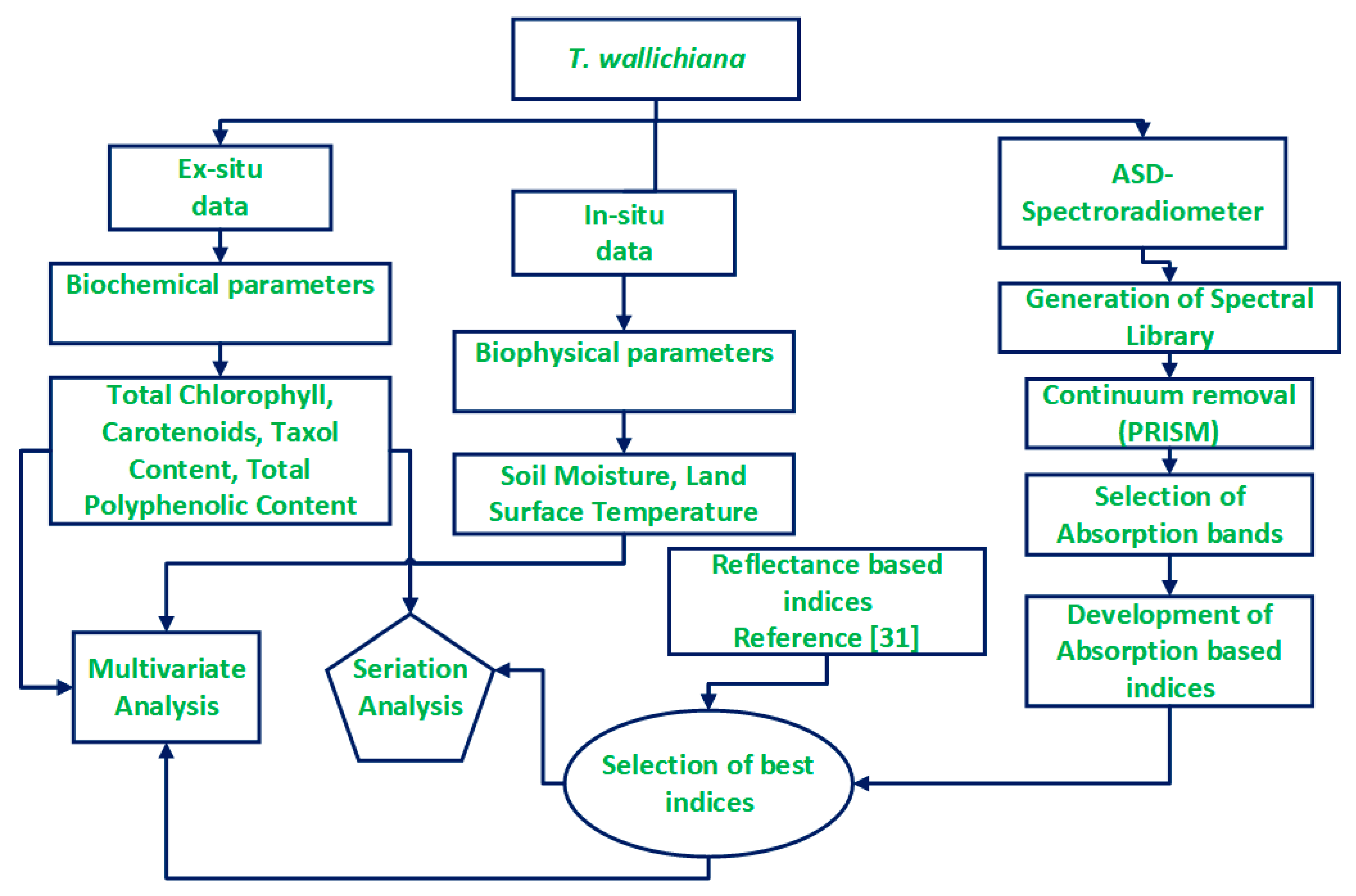
2. Materials and Methodology

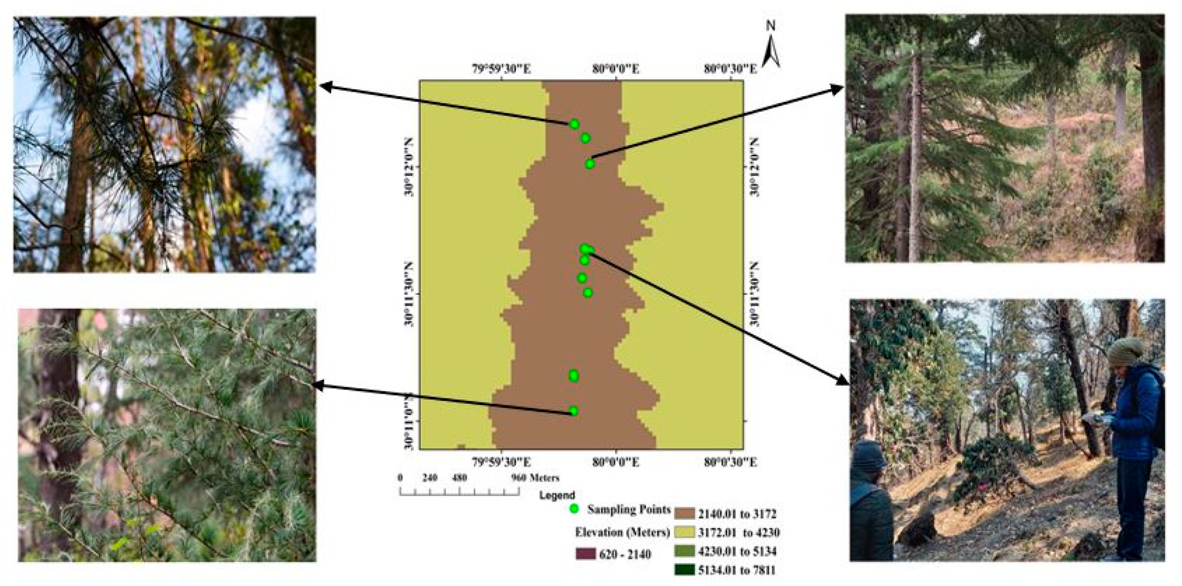
2.1. Study Area

Pindari glacier, which is situated in the Central Himalaya of Almora District of Uttaranchal state, was used as a study area for this research. Pindari glacier spread around the length of 5 km within an elevation range of 2400–3000 m. The climate of this region is categorized into the following three seasons: winters, summers, and monsoon. The long cold winter range from October to March with temperatures reaching below freezing point. In contrast, the maximum temperature seen in summers is around 30 °C. Mostly cloudy conditions exist throughout the monsoon months (June to September) because of the disturbances of western regions. The average annual rainfall is 930 mm, which mainly occurs during July and August [24]. Broadly, the area is divided into two climatic zones that could be categorized as (i) Lower montane zone: elevation range of 1800–2400 m above mean sea level (amsl), and (ii) Upper montane zone: elevation range of 2400–3000 m amsl. There is more precipitation in the upper zone and is more in terms of snowfall than showers [25]. The vegetation of the Pindari region comprises Pinus, Acer, Juglans, Cupressus, Quercus, Taxus, Berberis, and Rhododendron, which can be found around the region of Phurkia and the Pindari Glacier, as shown in Figure 1. This region is mostly covered by dense forests with high availability of medicinally important species [26,27,28]. The survey mainly focused on the collection of medicinally important species, i.e., Taxus wallichiana.

2.2. Sample and Radiometer Data Collection

The sample was collected on 26 September 2019 and 29 September 2019 at different locations along with a Global Positioning System (GPS) coordinate that varied between altitudes of 3039 and 2292 m in the Nanda Devi Biosphere Reserve (NDBR) in the state of Uttarakhand, which is located in the Western Himalayan Highland Biogeographic Zone. The samples were kept in a Ziploc bag for the next few hours. The samples collected were then crushed and stored in liquid nitrogen until the immediate analysis. Hence, all the values reported after analysis are represented in terms of fresh weight (FW).

The full range (350–2500 nm) FieldSpec spectroradiometer developed by Analytical spectral devices (ASD) was used to capture the spectral reflectance of the leaves and pre-processed using ViewSpecPro software Version 6.2 by Malvern Panalytical, Malvern, United Kingdom. ASD uses a fore-optic system to measure the spectral radiance and reflectance of any object. It distributes the signal via a fiber optic bundle to a fixed diffraction grating spectrometer. It uses three different types of detectors enabling a spectroradiometer to record the whole spectra from 350–2500 nm. Spectral reflectance is the part or a fraction of incident electromagnetic radiation that is reflected from any interface. The reflectance is plotted with a wavelength known as the reflectance spectrum or spectral reflectance curve, which is the end product of the device [29,30]. A Spectralon reference panel was used to optimize and adjust the sensitivity of the instrument.

2.3. Robustness of Indices

2.3.1. Reflectance Based Indices

A study was conducted on the Himalayan region for the development of the best Taxol indices [31]. Three different filtering techniques were applied, namely, Savitzky and Golay (S. Golay), Fast Fourier transformation, and Average Mean Filter, prior to feature selection. S. Golay uses simplified least-square-fit intricacy for smoothing. A mean filter takes the mean spectral value of nearest points within the considered window as the new value of the middle point of the window. The Fourier domain digital filter is a simple trapezoid characterized by four indices (N1, N2, N3, N4). Digital filtering is implemented simply by multiplying the Fourier domain signal by the appropriate filter function, that is, the signal points between N1 and N2 multiplied by y (value of the slope). The processed spectra after each filter application on T. wallichiana spectra were then applied with feature selection (first derivative). From the transformed spectra, the absorbance region at certain wavelengths was selected. The reflectance file of T. wallichiana spectra in text format, measured taxol content along with the wavelength selected were taken as inputs in the Automated Radiative Transfer Models Operator (ARTMO) model and the two band indices, suitable for TC estimation, were developed.

The indices developed using Average Mean smoothened wavelength, revealed a significant correlation with the measured taxol values. The five most appropriate taxol indices were selected which were developed by Average-Mean filtered wavelengths as listed in

Table 1. Selected Taxol indices from Gupta et al. where R is reflectance band [31].

SI No.	Reflectance Based Taxol Indices
1	TC 1 = (R426 − R421)/(R426 + R421)
2	TC 2 = (R415 − R421)/(R415 + R421)
3	TC 3 = (R601 − R608)/(R601 + R608)
4	TC 4 = (R421/R426)
5	TC 5 = (R415/R421)

.

Since taxol detection using hyperspectral data is not a phenomenon that has been explored much, all the wavelengths suggested by Gupta et al. [31] obtained from three different filtering techniques were considered. This was performed to rule out any possibilities of missing out even small absorption peaks that could indicate a taxol presence on hyperspectral data.

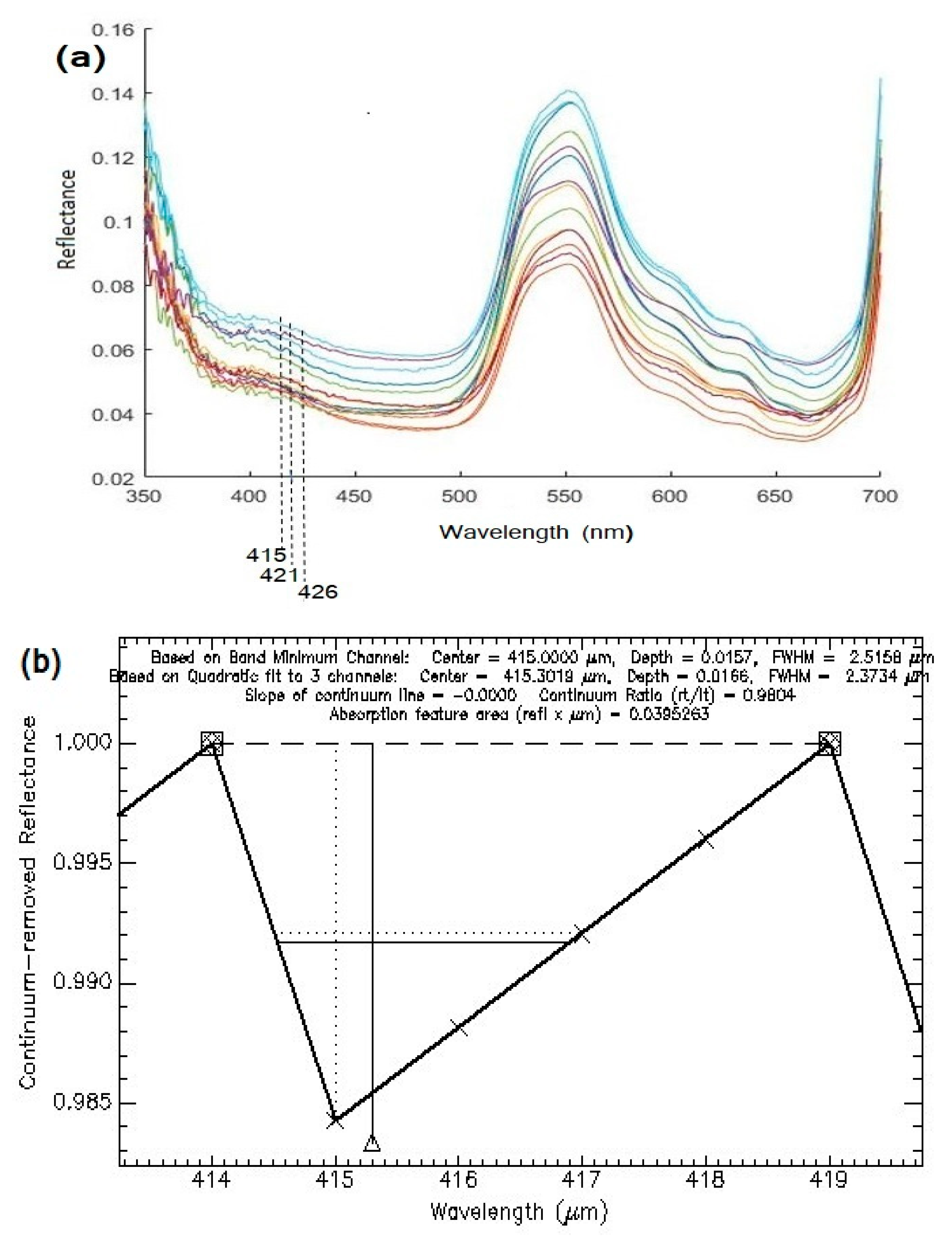
2.3.2. Absorption Based Indices

Continuum removal is referred to as baseline normalization and has been commonly used in laboratory infrared spectroscopy. This technique is an estimate of the other absorptions present in the spectrum. In that sense, continuum removal is most often performed on absorption features.

Continuum removal was applied to the selected absorption features. Continuum removal normalizes reflectance spectra in order to allow for a comparison of individual absorption features from a common baseline [32]. The continuum is a convex hull fitted over the top of a spectrum to connect the local spectrum maxima.

$$\mathrm{R}{\mathrm{c}}^{\prime }{}_{\left(\mathsf{\lambda }\mathrm{i}\right)}=\frac{{\mathrm{R}}_{\left(\mathsf{\lambda }\mathrm{i}\right)}}{{\mathrm{R}}_{\mathrm{c}}{}_{\left(\mathsf{\lambda }\mathrm{i}\right)}}$$

(1)

Here, in Equation (1), the continuum-removed reflectance is Rc′_(λi), the reflectance value is R_(λi) for each waveband in the absorption pit, and the reflectance level of the continuum line (convex hull) is R_{c (λi)} at the corresponding wavelength. The first and last spectral data values are on the hull and, therefore, the first and last values of the continuum removed spectrum is equal to 1. This process enhances the absorption pits’ output, whose values are between 0 and 1 [33]. Three variables were calculated from the continuum removed absorption features, viz. Continuum removed derivative reflectance (CRDR), band depths (BD), and band depth ratio (BDR). Collectively, this has been termed spectral feature analysis [34].

Processing Routines in IDL for Spectroscopy Measurements (PRISM) have the feature for automated spectral feature analysis [1]. Using this feature section option, the user can select the initial and final continuum endpoints on the spectrum to be analyzed. The PRISM software applies continuum removal to each spectrum separately and derives the spectral feature parameters (e.g., center, depth, width, area, etc.). PRISM performs continuum removal twice and gives the feature parameters as follows: (1) selection of start and endpoints; and (2) an automatically attuned set of continuum endpoints. PRISM searches for improved continuum endpoints on both sides of the absorption feature, by searching for nearby channels that have continuum-removed values higher than the initial endpoints. The new endpoint channels are referred to as the adjusted endpoints, as shown in Figure 2b. This software is added as an extension to ENVI 5.1 Aliso Viejo, CA, USA. This software can be downloaded from (https://pubs.usgs.gov/of/2011/1155/ accessed on 12 February 2021). This corresponding wavelength absorption feature area was used to develop absorption-based indices.

2.4. Soil Moisture and LST

The soil moisture (SM) and soil temperature are better known as Land Surface Temperature (LST). The in-situ measurements during sampling were carried out using Steven’s HydraGo instrument. HydraGo is a rugged SM sensor that measures the dielectric spectrum of the soil based on the ‘dielectric impedance’ at a 50 MHz radiofrequency (https://stevenswater.com/products/hydrago-s/ accessed on 12 February 2021). The reflected signals measure the soil dielectric permittivities that correspond to the SM and bulk soil electrical conductivity (EC). The device communicates wirelessly with the HydraMon app using Bluetooth. The app displays soil moisture content, temperature, conductivity, and dielectric permittivity for immediate viewing. The date and time of each measurement were recorded along with this measurement and the GPS location was measured using a handheld Garmin GPS receiver.

2.5. Determination of Chlorophyll (TCC), Total Phenolic Content (TPC), and Taxol Content (TC)

For the estimated total chlorophyll content (TCC), a crushed leaf sample was homogenized with 2 mL of acetone (80%) and then centrifuged for 10,000× rpm for 15 min at 4 °C. An amount of 0.5 mL of supernatant was taken from the main solution and mixed with 4.5 mL of acetone. The solution mixture was analyzed for chl. a, chl. b, and carotenoids using a spectrophotometer (Thermo scientific UV–Vis Spectrophotometer). The TPC in various plant samples was estimated using the Folin–Ciocalteu (F–C) colorimetric method. The plant leaf samples were added with 2 mL of ice-cold 95% (vol/vol) methanol and then were homogenized. The samples were kept in the dark for 48 hr. The samples were then centrifuged again (13,000× rpm for 5 min). To the 150 µL supernatant of this plant extract, 900 µL of distilled water was added, followed by 225 µL of F–C reagent, was added to the solution and it was permitted to stand still for 5 min at room temperature. Then, 1.125 mL of 2% sodium carbonate was added and mixed thoroughly. Along with the samples, the blank was also prepared without the supernatant plant extract but with the other entire constituent. The prepared samples and the blank were set aside in the dark for 15 min at room temperature. The absorbance of the samples and the blank were noted using a spectrophotometer @750 nm. The TPC was calculated with a standard curve based on gallic acid. The TPC results were expressed in milligrams of gallic acid equivalent (GAE) per gram fresh weight (FW) (mg GAE/g FW) [35,36].

For TC, 1 g of crushed leaves was deflated with hexane using sonication. The hexane portions were discarded, and aliquots of methanol were concentrated using a rotary evaporator, extracted in chloroform, then dried under reduced pressure using a rotary evaporator, and then re-dispersed in methanol (1 mL). Taxoid standard paclitaxel (Sigma, St. Louis, MI, USA) as used as a standard in HPLC for quantification. The working solution of paclitaxel was prepared from standard methanol. The UV-DAD scanned acquisitions of Taxol were performed at 230 nm. The percentage of Taxol was calculated using Equation (2) [37].

$$\mathrm{Taxol}(\%)\mathrm{Content}=\frac{\mathrm{Ar}{.}_{\mathrm{sample}}\times \mathrm{Conc}{.}_{\mathrm{std}.}\left(\raisebox{1ex}{$\mathrm{mg}$}\!\left/ \!\raisebox{-1ex}{$\mathrm{mL}$}\right.\right)}{\mathrm{Ar}{.}_{\mathrm{std}.}\ast 1000\times \mathrm{Conc}{.}_{\mathrm{sample}}\left(\raisebox{1ex}{$\mathrm{g}$}\!\left/ \!\raisebox{-1ex}{$\mathrm{mL}$}\right.\right)}\times 100$$

(2)

where Ar_std and Ar_sample are the areas under the peak associated with the standard or reference and sample taxoid, respectively, and Conc._sample and Conc._std are the concentrations of the sample and reference taxoid, respectively [37].

The standard methodology of collecting in-data and samples was followed as described earlier in Section 2.2 and Section 2.4. The samples of the plants underwent multiple tests (Section 2.5) for obtaining ex-situ data. The ASD spectroradiometer was used as an input to extract absorption values from the spectra of the T. wallichiana via PRISM software [31,32]. The absorption values were then used to develop two-band absorption indices. The measured taxol content along with selected bands, reflectance-based indices values, absorption-based indices values were subjected to Pearson correlation in R studio software Boston, MA, USA. It brings out the most suitable indices for taxol estimation. The measured TC along with the selected hyperspectral indices and ex-situ data were subjected to Pearson’s correlation to check their correlations. This step highlighted the correlation between the variable measured and the indices selected. Bartlett’s sphericity test was applied to the correlation matrix variables to test the assumption that variances are equal across groups. The elevation for the samples collected between 3039 and 2292 m was divided into three groups based on elevation, and One-way Analysis of Variance (ANOVA) was applied to test the significance of elevation with each set of parameters. ANOVA was followed by Scheffe’s test, which was applied to identify the significance of this difference among designated groups. PCA was done on SPSS Version 22 developed by IBM Armonk, New York, NY, USA. This further was applied to accomplish a significant reduction in the dimensionality of the original data set and bring the most varying variables to the foreground. Multivariate analysis was to highlighted the role of elevation and parameters for a suitable habitat for T. wallichiana. The flowchart depicting the methodology is shown in Figure 3.

3. Results and Discussion

3.1. Comparative Analysis between Indices, Selected Wavelengths, and Measured Taxol Content

The absorption indices were developed using two-band absorption values in different combinations. More than 84 absorption indices combinations were tested using the two bands. While these combinations were tried in the preliminary stage, it was observed that the indices utilizing the bands 415 and 670 nm outperformed any other indices developed utilizing other wavelengths. The indices with significant correlation are plotted in Figure 4, in what is known as a correlogram. A correlogram or Auto Correlation function is a visual way to show the serial correlation in data that change over time.

Figure 4 illustrates the correlation among all the possible absorption band values along with the absorption and reflectance indices values that showed a significant correlation with the taxol content. The absorbance wavelengths are represented with ‘x’ as a subscript and the absorption indices values are represented with ‘i’, while the reflectance-based indices are represented with TC. Figure 4 shows that the measured taxol content (Ob) showed the nearest positive correlation with reflectance-based indices TC 2 (r = 0.741) and TC5 (r = 0.742). The Ob values also showed a positive correlation with absorption indices Ni (r = 0.565) and Mi (r = 0.561), while a significant negative correlation was observed between Ob and Ri (r = 0.604) and Oi (r = −0.615). The parameters Si, Pi, and Qi also showed a significant positive correlation but the magnitude values were out of range; hence, they were discarded. In a general sense, the absorption-based indices showed a significant correlation, but the indices were more likely to capture the trend of the real values rather than quantifying near the measured taxol values. In contrast, the reflectance-based indices captured trends along with the magnitude of the real values. The reflectance-based indices (TC 2 and TC 5) showed the highest correlation to the measured taxol content (Ob). The wavelength absorption values that were found most closely to the Ob values were Bx and Dx, which are centered at 415 and 670 nm, respectively. The positive correlating factors to the Ob values were majorly allocated in the center of Figure 4, which implies that the difference between the modelled and observed values was found the least in terms of magnitude. The center region of the graph majorly consists of indices values, either reflectance-based or absorption-based. This highlights the fact that to exploit hyperspectral data, more techniques need to be explored to process the data. The correlation heat map as per [4] may indicate the metabolite signature on the spectra, but to make those data useful information, more techniques need to be implemented.

The absorption indices that show a significant correlation and a magnitude value within the range, as compared to the measured TC, are listed in

Table 2. Selected Taxol absorption-based indices where R is reflectance band.

SI No.	Absorption Based Taxol Indices
1	Ni = (R415 − R670)/(R415 + R670)
2	Mi = (R415 − R2272)/(R415 + 2272)
3	Ri = R670/R1181
4	Oi = R670/R975

. Since the reflectance-based indices outperformed any other indices and wavelengths, they were further considered for the next set of statistical operations along with other important variables.

3.2. Descriptive Statistics

The land surface temperature (LST) showed a slightly higher temperature at the low altitude of around 15.8 (°C) at an elevation of 2992 m. With the varying altitude, the temperature also changed. The samplings were conducted in the rainy season with the average LST recorded as 14.171 $\pm$ 1.002 (°C). By following the soil temperature, the soil moisture values show a mean value of 43.950 $\pm$ 5.500 (%). The final values show that the TC varied between 0 and 0.037 mg/g FW, with an average of 0.011 mg/g FW ± 0.012. The values of total phenolic content (TPC) ranged from 72.656 to 94.676 mg GAE/g FW, with an average value of 79.973 ± 6.418. The correlation concerning elevation for TPC was found to be 0.672, which is significant. This shows that the TPC shows a clear positive change with elevation (as in

Table 3. Pearson’s correlation matrix among edaphic parameters, topographic parameters, biochemical- and indices-generated parameters of Taxus wallichiana needles.

Variables	Elevation	SM	Taxol Content	TCC	Carotenoids	TPC	LST	TC 1	TC 2	TC 3	TC 4	TC 5
Elevation	1.000
SM	0.333	1.000
Taxol content	0.277	−0.478	1.000
TCC	−0.238	−0.340	0.186	1.000
Carotenoids	0.435	0.065	0.333	−0.162	1.000
TPC	0.658	0.516	−0.070	−0.438	0.001	1.000
LST	−0.445	−0.654	0.478	0.312	−0.080	−0.533	1.000
TC 1	0.789	0.192	0.495	0.087	0.456	0.380	−0.158	1.000
TC 2	0.372	−0.186	0.715	0.310	0.508	−0.116	0.401	0.656	1.000
TC 3	−0.393	−0.296	0.341	0.104	0.168	−0.543	0.536	−0.218	0.304	1.000
TC 4	0.782	0.188	0.497	0.090	0.454	0.379	−0.153	1.000	0.658	−0.219	1.000
TC 5	0.357	−0.191	0.715	0.313	0.504	−0.122	0.410	0.646	1.000	0.311	0.648	1.000

). It clearly shows that medicinal plants also carry phenolic content in them, which indirectly shows the redox properties that are responsible for their antioxidant properties. The p-value was 0.006, which is also less than 0.05. This clearly shows that there is not much of a significant difference among the TPC content values, but it does increase with the elevation. The total polyphenol content (TPC) has a positive correlation with elevation, while it shows a negative correlation with the temperature. TPC is not limited by ecosystem boundaries but limited by human interventions. TPC values do increase with elevation. The high TPC concentration reported in T. wallichiana suggests that the medicinal plant contains high antioxidant activity, which makes it more beneficial.

The total chlorophyll content (TCC) values vary from 2.013 to 4.194 mg/g. The average total chlorophyll concentration was found to be 3.541 ± 0.504. The correlation of total chlorophyll content with elevation came out to be insignificant. Similarly, the correlation between total chlorophyll and taxol was found to be insignificant. The values for carotenoids vary between 0.703 to 0.982 mg/g. The average carotenoid value came out to be 0.836 ± 0.087. This correlation between elevation and carotenoid was found to be insignificant (Table 3). The correlation between total chlorophyll and carotenoids was statistically insignificant. This inverse relationship between chlorophyll and carotenoid directs toward the inference that carotenoids increase in the senescence stage and chlorophyll is reported to be higher than carotenoids in the growing period in the case of many plants [38].

TPC shows a significant positive correlation with Soil Moisture (SM) of 0.516 and a significant negative correlation with LST. Soil Moisture shows an inverse relationship with LST, which is obvious as the temperature is the driving factor for water movement [39]. Here, the TPC relationship clearly indicates that TPC is affected by temperature [40].

The correlation matrix between the parameters of indices from TC 1 to TC 5 with elevation verifies the fact that the reflectance/albedo varies at different altitudes. This indicates that the indices developed for biochemical factors have the effect of altitude within them. Similarly, Mokarram et al. [41] have indicated that the vegetation growth is highest between the elevations of 1500 to 3000 m, with high values of the Normalized Difference Vegetation Index (NDVI), the Enhanced Vegetation Index (EVI), and the Difference Vegetation Index (DVI). It can be seen that TC 1 shows a clear relationship with TC 2 and TC 5 while TC 2 correlates with TC 4, but all these indices are probable indices for the same parameter, i.e., taxol. Hence, their mutual correlation is expected. Although, it is noticeable that TC 2 shows a perfect correlation with TC 5, and both TC 2 and TC 5 show the highest correlation with Taxol, which indicates that both the indices are useful in calculating Taxol content using hyperspectral reflectance data. TC 2 and TC 5 also show correlation with carotenoids, but the correlation cannot be considered significant. In the correlation matrix in Table 3, it can be seen that neither TC 2 nor TC 5 showed any significant correlation with any other foliar characteristic than taxol nor the taxol indices. This showed that the taxol indices developed using the wavelength of the visible region (415 and 421 nm) can be uniquely characterized for the same. Taxol did not show any significant correlation with elevation directly. Similar results were also obtained for taxol by Priyanka et al. After the application of ANOVA, the null hypothesis was accepted for soil moisture, total chlorophyll, near-surface temperature, taxol content, and carotenoids. The null hypothesis was rejected for TPC based on the Fcrit and p-value. The F values of 13.875 exceed the critical value of 3.88, which signifies that there is a difference among groups. Pairwise Scheffe’s showed that there is no statistical significance among the various classes for TPC based on elevation.

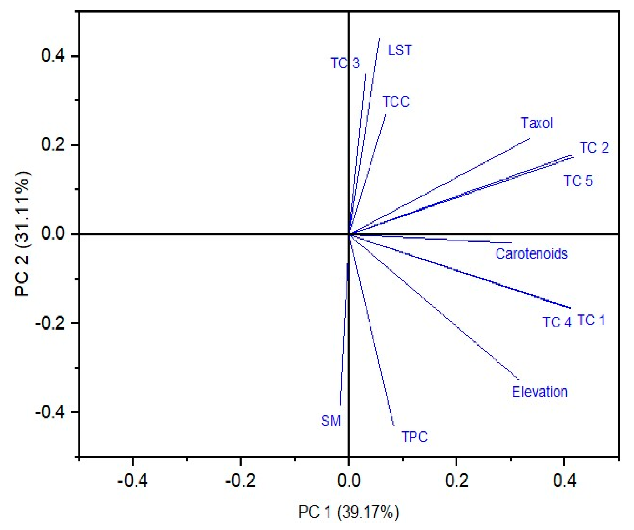
3.3. Multivariate Analysis

Bartlett’s sphericity test shows a calculated χ² = 243.932, which is greater than the critical value χ² = 22.362 (p = 0.05), thus the null hypothesis of equal variance among groups was rejected, indicating that PCA can accomplish a significant reduction in the dimensionality of the original data set [42]. To determine the principal component that explains the major attributes of T. wallichiana, PCA was applied, as shown in

Table 4. Loadings of experimental variables on the PCs for the combined data set of Taxus wallichiana (red indicates the most significant component).

Variables	PC 1	PC 2	PC 3
Elevation	0.684	0.630	−0.021
Soil Moisture (SM)	−0.036	0.743	0.179
Measured Taxol content (Taxol)	0.727	−0.417	0.009
Total Chlorophyll content (TCC)	0.147	−0.522	−0.697
Carotenoids	0.652	0.035	0.532
Total Polyphenolic Content (TPC)	0.179	0.828	0.036
Land Surface Temperature (LST)	0.122	−0.850	0.001
TC1	0.891	0.321	−0.205
TC2	0.902	−0.337	0.053
TC3	0.066	−0.700	0.512
TC4	0.891	0.317	−0.208
TC5	0.896	−0.347	0.055
Eigen Value	4.700	3.733	1.155
% Variance	39.17%	31.11%	9.63%
Cumulative % Variance	39.17%	70.28%	79.91%

and Figure 5.

PCA was performed on the combined (edaphic, topographic, and biochemical properties, and indices values) correlation matrix dataset in order to identify a condensed set of features that could capture and explain most of the variance in the data for T. wallichiana. The Scree plot and Table 4 highlight the factor loadings, eigenvalues, and variance described by each PC. According to the criteria set by [43], an eigenvalue greater than one was considered as a principal component. The factor loading of more than 0.650 was considered a contributing factor since the sample size was less than 100. PCA rendered three principal components with eigenvalues > 1, explaining almost 80.00% of the total variance of the data. The parameter PC 1, describing 39.17%, has strong positive factor loadings (>0.80) on TC 1, TC 2, TC 4, and TC 5. PC 1 also shows moderate loadings for the measured taxol content (>0.70) and elevation (>0.65), thus highlighting that taxol and elevation are the most varying variables among the measured parameters. In the case of T. wallichiana, the TC varies with age and seasons; hence, this variance is expected [44,45]. PC 2 explained 31.11% of the total variance and has moderate negative loading on LST. PC 2 also shows strong positive loading with TPC and SM. The loadings and scores of the first two PCs (PC1 and PC2) are plotted in Figure 5. The loadings plot (Figure 5) shows the distribution of all the parameters in the first (upper right) and fourth (lower right) quadrants. The factor loading lines joining the variables along with the length of the line passing through the origin in the plot of the factor loadings are indicative of the low and high contribution of the variables to the samples. The closeness of the lines of two variables signifies the strength of their mutual correlation, which was also adequately shown using a correlation matrix. The assemblage of TC, Carotenoids, elevation, TPC, and SM in the loadings plot suggests their significant mutual positive correlation.

3.4. Seriation Analysis

Generally, as the amount of medicinal compound is dependent upon numerous factors, it primarily involves elevation, temperature, and the ecosystem. Here, seriation was conducted to bring out the arrangement of various factors related to TC. The relationship becomes highly subjective but has some principal components that are commonly associated with biochemical parameters. The results of this study suggest that a landscape variable such as altitude is important in influencing other biochemical parameters as well as the secondary metabolites associated with the selected species. In order to analyze the data more clearly, the seriation plot and dendrogram were generated and are shown in Figure 6. The samples at every 50 m were pooled together as one sample. The objective functions during the iteration for the row and the column were obtained as 0.707 and 0.644, respectively, while the sum of all the pairwise distances in the neighboring rows (path length) was found to be 43.484 and the neighboring column (path length) was found to be 31.869. The Complete linkage rule was utilized for both the row and column, while the multi fragment heuristic (MF) scaling rule was used for tree seriation. The dissimilarity analysis used in seriation was based on the Euclidean distance measurement.

The seriation column matrix plot Cluster C4 contains TPC and SM, while cluster C5 contains carotenoids and elevation along with TC 1 (Index 1) and TC 4 (Index 4). This implies that the elevation, TPC, SM, and Carotenoids values show a relation with TC 1 and TC 4. This implies that elevation, due to the change in albedo, has a direct relationship with biochemical and edaphic properties. The C6 cluster contains TC3 (Index 3), LST, Taxol, TC 2 (Index 2), and TC 5 (Index 5). Carotenoids show a close relationship with both indices-generated values TC 4 and TC 3. Similarly, the Taxol content was found to be feeble with LST, but the correlation coefficient was insignificant to consider. The taxol content has a close correlation with TC 2 and TC 5 with good correlation values and does not relate to any other variable, even in the hierarchical sense. Hence, it can be said that TC 2 and TC 5 can only retrieve taxol, not any other common foliar pigment found in the visible region of electromagnetic spectra. The Total Chlorophyll Content (TCC) behaved as a runt. It consistently showed the same range values without being majorly affected by any other variable. The TCC is supposed to vary with the season, species, age of the plant, and forest type [46].

The samples S6, S8, S10, S4, S5, S3, and S9 are grouped in one cluster, C1, while cluster C2 includes samples S7, S12, S11, and S2. Samples S14 and S15 clustered together in C3. In Figure 6, several samples from cluster C1 were characterized with similar behavior. These samples were measured in-between altitudes of 2826 and 3003 m, which is also the dense region of the forest in the sampling area. Therefore, these samples must have a strong influence on the forest and its ecosystem. The samples clustered under C2 and C3 shared the same hierarchy, due to their presence either at the high or low altitude of the sampling elevation, which was marked by human intervention at the lower altitude or ecosystem change at the higher altitude.

4. Conclusions

The reflectance-based indices are more useful in quantifying taxol content using hyperspectral data. More techniques such as indices and algorithms need to be applied for the exploitation of hyperspectral data so that these data can be converted into useful information, as absorption bands at particular wavelengths are not providing any sufficient information to make the HSR data more useful. In the case of multispectral satellite data, absorption-based indices may be used to quantify the taxol content.

The result of statistical analysis suggests that the density of the forest determines the range of parameters measured, which, in the case of the montane ecosystem, is indirectly determined by elevation. Therefore, elevation along with aspect and slope in many respects determines the microclimate, and thus, plays an important role in foliar and edaphic properties in the case of the montane ecosystem. Chlorophyll does not show any significant change in a species under the same forest canopy therefore, it might be used as a health indicator at the canopy scale but cannot be used as an indicator to decide the number of secondary metabolites in the same species.

The relationship in the case of taxol with elevation suggests that the taxol content does not vary with elevation but is affected by temperature. It is the most varying variable among the measured variables, followed by elevation and carotenoids. The frequency of the plant becoming less near the edge of the ecosystem (ecotone) and the amount of taxol content in T. wallichiana near these regions was also low. Beyond 3100 m, more of a grassland ecosystem exists in the NDBR. The samples showing similar behavior in terms of parameters were found between elevations of 2800 to 3000 m in the NDBR. This region is characterized by dense forests in the NDBR. The T. wallichiana plant shows low taxol content near the timberline at Phurkia and near the point of human intervention at Khati (the last habitable point in the valley). This makes our understanding of this highly medicinal plant more refined. T. wallichiana with a high taxol content is found more in its natural habitat in the absence of human intervention and ecosystem change. Taxol indices TC 2 and TC 5, which were developed using visible range wavelengths (415 and 421 nm) of the hyperspectral data, have been related to the taxol content and not related with other foliar variables, which might be attempted in the future. This study can be expanded to other regions for taxol estimation, but the availability of ground hyperspectral data is a challenge. The canopy chemistry and its relationship with remote sensing hyperspectral data is a challenge, as there are thousands of compounds in the same species. The implementation of more sophisticated techniques applied with HSR holds the key to future research in canopy chemistry.

References

1. Kokaly, R.F.; Skidmore, A.K. Plant phenolics and absorption features in vegetation reflectance spectra near 1.66 μm. Int. J. Appl. Earth Obs. Geoinf. 2015, 43, 55–83. [Google Scholar] [CrossRef] [Green Version]
2. Lu, B.; He, Y.; Liu, H.H. Mapping vegetation biophysical and biochemical properties using unmanned aerial vehicles-acquired imagery. Int. J. Remote Sens. 2018, 39, 5265–5287. [Google Scholar] [CrossRef]
3. Peng, Y.; Zhang, M.; Xu, Z.; Yang, T.; Su, Y.; Zhou, T.; Wang, H.; Wang, Y.; Lin, Y. Estimation of leaf nutrition status in degraded vegetation based on field survey and hyperspectral data. Sci. Rep. 2020, 10, 1–12. [Google Scholar] [CrossRef] [PubMed] [Green Version]
4. Fine, P.V.; Salazar, D.; Martin, R.E.; Metz, M.R.; Misiewicz, T.M.; Asner, G.P. Exploring the links between secondary metabolites and leaf spectral reflectance in a diverse genus of Amazonian trees. Ecosphere 2021, 12, e03362. [Google Scholar] [CrossRef]
5. Hui, C. Carrying capacity, population equilibrium, and environment’s maximal load. Ecol. Model. 2006, 192, 317–320. [Google Scholar] [CrossRef]
6. Asner, G.P.; Martin, R.E. Conservation. Spectranomics: Emerging science and conservation opportunities at the interface of biodiversity and remote sensing. Glob. Ecol. 2016, 8, 212–219. [Google Scholar] [CrossRef] [Green Version]
7. Jugran, A.K.; Bahukhandi, A.; Dhyani, P.; Bhatt, I.D.; Rawal, R.S.; Nandi, S.K. Impact of altitudes and habitats on valerenic acid, total phenolics, flavonoids, tannins, and antioxidant activity of Valeriana jatamansi. Appl. Biochem. 2016, 179, 911–926. [Google Scholar] [CrossRef]
8. Díaz, S.; Kattge, J.; Cornelissen, J.H.; Wright, I.J.; Lavorel, S.; Dray, S.; Reu, B.; Kleyer, M.; Wirth, C.; Prentice, I.C. The global spectrum of plant form and function. Nature 2016, 529, 167–171. [Google Scholar] [CrossRef] [PubMed]
9. Nisar, M.; Khan, I.; Simjee, S.U.; Gilani, A.H.; Perveen, H. Anticonvulsant, analgesic and antipyretic activities of Taxus wallichiana Zucc. J. Ethnopharmacol. 2008, 116, 490–494. [Google Scholar] [CrossRef] [PubMed]
10. Shi, Q.W.; Kiyota, H. New natural taxane diterpenoids from Taxus species since 1999. Chem. Biodivers. 2005, 2, 1597–1623. [Google Scholar] [CrossRef] [PubMed]
11. Kumari, N.; Srivastava, A.; Dumka, U.C. A long-term spatiotemporal analysis of vegetation greenness over the Himalayan Region using Google Earth Engine. Climate 2021, 9, 109. [Google Scholar] [CrossRef]
12. Lin, D.; Xiao, M.; Zhao, J.; Li, Z.; Xing, B.; Li, X.; Kong, M.; Li, L.; Zhang, Q.; Liu, Y. An overview of plant phenolic compounds and their importance in human nutrition and management of type 2 diabetes. Molecules 2016, 21, 1374. [Google Scholar] [CrossRef]
13. Hill, J.; Buddenbaum, H.; Townsend, P.A. Imaging spectroscopy of forest ecosystems: Perspectives for the use of space-borne hyperspectral earth observation systems. Surv. Geophys. 2019, 40, 553–588. [Google Scholar] [CrossRef]
14. Shang, X.; Chisholm, L.A. Classification of Australian native forest species using hyperspectral remote sensing and machine-learning classification algorithms. IEEE J. Sel. Top. Appl. Earth Obs. Remote Sens. 2013, 7, 2481–2489. [Google Scholar] [CrossRef]
15. Anand, A.; Pandey, M.K.; Srivastava, P.K.; Gupta, A.; Khan, M.L. Integrating Multi-Sensors Data for Species Distribution Mapping Using Deep Learning and Envelope Models. Remote Sens. 2021, 13, 3284. [Google Scholar] [CrossRef]
16. Zarco-Tejada, P.J.; Morales, A.; Testi, L.; Villalobos, F. Spatio-temporal patterns of chlorophyll fluorescence and physiological and structural indices acquired from hyperspectral imagery as compared with carbon fluxes measured with eddy covariance. Remote Sens. Environ. 2013, 133, 102–115. [Google Scholar] [CrossRef]
17. Li, F.; Miao, Y.; Feng, G.; Yuan, F.; Yue, S.; Gao, X.; Liu, Y.; Liu, B.; Ustin, S.L.; Chen, X. Improving estimation of summer maize nitrogen status with red edge-based spectral vegetation indices. Field Crop. Res. 2014, 157, 111–123. [Google Scholar] [CrossRef]
18. Wu, C.; Niu, Z.; Tang, Q.; Huang, W. Estimating chlorophyll content from hyperspectral vegetation indices: Modeling and validation. Agric. For. Meteorol. 2008, 148, 1230–1241. [Google Scholar] [CrossRef]
19. Singh, P.; Srivastava, P.K.; Malhi, R.K.M.; Chaudhary, S.K.; Verrelst, J.; Bhattacharya, B.K.; Raghubanshi, A.S. Denoising AVIRIS-NG data for generation of new chlorophyll indices. IEEE Sens. J. 2020, 21, 6982–6989. [Google Scholar] [CrossRef]
20. Wang, Z.; Wang, T.; Darvishzadeh, R.; Skidmore, A.K.; Jones, S.; Suarez, L.; Woodgate, W.; Heiden, U.; Heurich, M.; Hearne, J. Vegetation indices for mapping canopy foliar nitrogen in a mixed temperate forest. Remote Sens. Environ. 2016, 8, 491. [Google Scholar] [CrossRef] [Green Version]
21. Ollinger, S.V.; Richardson, A.D.; Martin, M.E.; Hollinger, D.Y.; Frolking, S.E.; Reich, P.B.; Plourde, L.C.; Katul, G.G.; Munger, J.W.; Oren, R. Canopy nitrogen, carbon assimilation, and albedo in temperate and boreal forests: Functional relations and potential climate feedbacks. Proc. Natl. Acad. Sci. USA 2008, 105, 19336–19341. [Google Scholar] [CrossRef] [PubMed] [Green Version]
22. Fernandes, M.R.; Aguiar, F.C.; Silva, J.M.; Ferreira, M.T.; Pereira, J.M. Spectral discrimination of giant reed (Arundo donax L.): A seasonal study in riparian areas. ISPRS J. Photogramm. Remote Sens. 2013, 80, 80–90. [Google Scholar] [CrossRef]
23. Hennessy, A.; Clarke, K.; Lewis, M.J.R.S. Hyperspectral classification of plants: A review of waveband selection generalisability. Remote Sens. 2020, 12, 113. [Google Scholar] [CrossRef] [Green Version]
24. Pandey, S.K.; Singh, A.K.; Hasnain, S. Grain-size distribution, morphoscopy and elemental chemistry of suspended sediments of Pindari Glacier, Kumaon Himalaya, India. Hydrol. Sci. J. 2002, 47, 213–226. [Google Scholar] [CrossRef] [Green Version]
25. Saxena, K.; Maikhuri, R.; Rao, K.; Nautiyal, S. Assessment Report: Nanda Devi Biosphere Reserve, Uttarakhand, India as a Baseline for Further Studies Related to the Implementation of Global Change in Mountain Regions (GLOCHAMORE) Research Strategy; Assessment Report; UNESCO, New Delhi Office: New Delhi, India, 2010. [Google Scholar]
26. Joshi, S.; Upreti, D.K. Lichenometric studies in vicinity of Pindari Glacier in the Bageshwar district of Uttarakhand, India. Curr. Sci. 2010, 99, 231–235. [Google Scholar]
27. Singh, R.; Kumar, S.; Kumar, A. Climate change in Pindari region, Central Himalaya, India. In Climate Change, Glacier Response, and Vegetation Dynamics in the Himalaya; Springer: Berlin/Heidelberg, Germany, 2016; pp. 117–135. [Google Scholar]
28. Joshi, S.; Upreti, D.; Das, P. Lichen diversity assessment in Pindari glacier valley of Uttarakhand, India. Geophytology 2011, 41, 25–41. [Google Scholar]
29. Mac Arthur, A.; MacLellan, C.J.; Malthus, T. The fields of view and directional response functions of two field spectroradiometers. IEEE Trans. Geosci. Remote Sens. Environ. 2012, 50, 3892–3907. [Google Scholar] [CrossRef]
30. Srivastava, P.K.; Malhi, R.K.M.; Pandey, P.C.; Anand, A.; Singh, P.; Pandey, M.K.; Gupta, A. Revisiting hyperspectral remote sensing: Origin, processing, applications and way forward. In Hyperspectral Remote Sensing; Elsevier: Amsterdam, The Netherlands, 2020; pp. 3–21. [Google Scholar]
31. Gupta, A.; Singh, P.; Srivastava, P.K.; Pandey, M.K.; Anand, A.; Chandra Sekar, K.; Shanker, K. Development of hyperspectral indices for anti-cancerous Taxol content estimation in the Himalayan region. Geocarto Int. 2021, 1–14. [Google Scholar] [CrossRef]
32. Kokaly, R.F. Investigating a physical basis for spectroscopic estimates of leaf nitrogen concentration. Remote Sens. Environ. 2001, 75, 153–161. [Google Scholar] [CrossRef]
33. Schmidt, K.; Skidmore, A. Exploring spectral discrimination of grass species in African rangelands. Int. J. Remote Sens. 2001, 22, 3421–3434. [Google Scholar] [CrossRef]
34. Schmidt, K.; Skidmore, A. Spectral discrimination of vegetation types in a coastal wetland. Remote Sens. Environ. 2003, 85, 92–108. [Google Scholar] [CrossRef]
35. Kamboj, A.; Gupta, R.; Rana, A.; Kaur, R. Application and analysis of the Folin Ciocalteu method for the determination of the total phenolic content from extracts of Terminalia bellerica. Eur. J. Biomed. Pharm. Sci. 2015, 2, 201–215. [Google Scholar]
36. Gupta, A.; Lamba, P.; Gupta, D.; Verma, D. Medicinal Evaluation of different flowers from Asteraceae Family. Bull. Environ. Sci. Res. 2019, 8, 10–14. [Google Scholar]
37. Shanker, K.; Negi, A.S.; Chattopadhyay, S.K.; Sashidhara, K.; Kaur, T.; Gupta, M.; Agrawal, P.; Misra, A. Determination of paclitaxel, 10-DAB, and related taxoids in Himalayan Yew using reverse phase HPLC. J. Herbs Spices Med. Plants 2008, 13, 25–44. [Google Scholar] [CrossRef]
38. Croft, H.; Chen, J.; Wang, R.; Mo, G.; Luo, S.; Luo, X.; He, L.; Gonsamo, A.; Arabian, J.; Zhang, Y. The global distribution of leaf chlorophyll content. Remote Sens. Environ. 2020, 236, 111479. [Google Scholar] [CrossRef]
39. Cuo, L.; Zhang, Y.; Bohn, T.J.; Zhao, L.; Li, J.; Liu, Q.; Zhou, B. Frozen soil degradation and its effects on surface hydrology in the northern Tibetan Plateau. J. Geophys. Res. Atmos. 2015, 120, 8276–8298. [Google Scholar] [CrossRef] [Green Version]
40. Ghaderpour, E.; Ben Abbes, A.; Rhif, M.; Pagiatakis, S.D.; Farah, I.R. Non-stationary and unequally spaced NDVI time series analyses by the LSWAVE software. Int. J. Remote Sens. 2020, 41, 2374–2390. [Google Scholar] [CrossRef]
41. Mokarram, M.; Sathyamoorthy, D. Modeling the relationship between elevation, aspect and spatial distribution of vegetation in the Darab Mountain, Iran using remote sensing data. Modeling Earth Syst. Environ. 2015, 1, 1–6. [Google Scholar] [CrossRef]
42. Vorapongsathorn, T.; Taejaroenkul, S.; Viwatwongkasem, C. A comparison of type I error and power of Bartlett’s test, Levene’s test and Cochran’s test under violation of assumptions. Songklanakarin J. Sci. Technol. 2004, 26, 537–547. [Google Scholar]
43. Singh, K.P.; Malik, A.; Sinha, S.; Singh, V.K.; Murthy, R.C. Estimation of source of heavy metal contamination in sediments of Gomti River (India) using principal component analysis. Water Air Soil Pollut. 2005, 166, 321–341. [Google Scholar] [CrossRef]
44. Nadeem, M.; Rikhari, H.; Kumar, A.; Palni, L.; Nandi, S. Taxol content in the bark of Himalayan Yew in relation to tree age and sex. Phytochemistry 2002, 60, 627–631. [Google Scholar] [CrossRef]
45. Yang, L.; Zheng, Z.-S.; Cheng, F.; Ruan, X.; Jiang, D.-A.; Pan, C.-D.; Wang, Q. Seasonal dynamics of metabolites in needles of Taxus wallichiana var. mairei. Molecules 2016, 21, 1403. [Google Scholar] [CrossRef] [PubMed] [Green Version]
46. Li, Y.; He, N.; Hou, J.; Xu, L.; Liu, C.; Zhang, J.; Wang, Q.; Zhang, X.; Wu, X. Factors influencing leaf chlorophyll content in natural forests at the biome scale. Front. Ecol. Evol. 2018, 6, 64. [Google Scholar] [CrossRef] [Green Version]
Figure 1. Sampling locations of T. wallichiana in Nanda Devi Biosphere Reserve.
Forests 12 01726 g001
Figure 2. Spectral feature analysis (a) sectional view of the spectra highlighting small dip (b) dip (feature) center position with feature depth and width highlighted after application of continuum removal for a single sample spectrum.
Forests 12 01726 g002
Figure 3. Flowchart for methodology opted for the current work.
Forests 12 01726 g003
Figure 4. Pearson’s correlation between the selected wavelength represented as ‘x’ as a subscript, absorption indices represented with ‘i’ as a subscript, and measured TC represented as ‘Ob’.
Forests 12 01726 g004
Figure 5. Loading plot of Principal Component Analysis for Taxus wallichiana.
Forests 12 01726 g005
Figure 6. Seriation Analysis of the samples.
Forests 12 01726 g006