Environment Status Estimation of the Forest Communities Based on Floristic Surveys in the Mordovia State Nature Reserve, Russia

Abstract

Environmental scales include species responsive to changes in environmental conditions. The present paper aims to apply floristic survey data to reveal environmental conditions in habitats studied in the Mordovia State Nature Reserve, European Russia. In total, 161 square plots were established within a selected forest area. In each plot, all species were registered to conduct a further analysis. Then, average values of six environmental factors were calculated based on the Tsyganov environmental scale. Contour maps were created for four factors to demonstrate spatial changes through the study area. All study pots were assigned to seven habitat types during the field surveys. To test the correctness of the determined classification, a principal component analysis was performed based on Tsyganov’s environmental factors. Additionally, PERMANOVA was used to test the correctness of the habitat distinguishing. The results demonstrate that differences in environmental conditions among the majority (mires, coniferous forests, broadleaved forests, mixed forests) of the distinguished habitats are statistically significant, except for water bodies, forest gaps and roads, which have no significant differences in environmental factors compared with other habitats. We assume that this is caused by the very small sampling size for these habitat types. To obtain correct results, each habitat group should be represented by at least 3–4% samples of the whole sampling set. The main conclusion represents a simple way to assess the habitat environmental status based on floristic data. Based on Tsyganov’s environmental factors, the spatial distribution of only plant specialists can be recognised well. The allocation of plant generalists is impossible based on the proposed approach. Finally, the correctness of habitat classification based on dominated plants is well-testable using environmental conditions found on these sites. We also recommend the use of the here applied approach in plant ecology studies in the subzone of coniferous–deciduous forests of Eastern Europe.

1. Introduction

Populations of plants are distributed regarding habitat conditions [1]. Depending on the environmental conditions, plant abundance and distribution, as well as the structure and floristic composition of plant communities, vary considerably [2,3,4,5]. Climatic and edaphic factors strongly influence the structure and composition of the vegetation cover [6,7,8,9]. Among them, the impact of climatic factors is most considerable at large scales [10], while habitat characteristics play an important role at a local scale [2,11,12,13]. Environmental factors related to the heterogeneity of small-scale landscapes (e.g., light availability and soil properties) are well-suited for studies at a local scale [14].

Environmental and phytogeographical gradients form the base of most vegetation classifications. They are used for the developing and functioning of various environmental scales [15,16,17,18,19]. Among them, interval-based environmental scales characterise synecological preferences of plants [16,19]. Tsyganov’s [16] scale is well-suitable for use in the zone of coniferous–broadleaved forests of European Russia [20,21]. Such environmental scales serve as a highly suitable tool for understanding a habitat’s environmental status (e.g., climatic, soil and illumination conditions), especially if any direct measurements are impossible or difficult [22,23]. In such a way, plant species are useful for indicating and mapping the gradients of the habitat’s environmental conditions based on the presence of a set of plant species using a phytoindication approach. This could be especially important when encountering an area preferred by certain threatened plants, which are generally specialists, usually typical for specific and sometimes harsh environments.

In this paper, we aim to use floristic survey data to evaluate the habitat environmental conditions in a model area in the centre of European Russia (the Mordovia State Nature Reserve). The main objectives are (i) to evaluate the relationships between plant dominant-based habitats and their environmental conditions based on Tsyganov’s [16] scale and (ii) to find a suitable way for analysing the spatial distribution of environment factor gradients based on the floristic composition of the studied plots. We hypothesise that the joint use of environmental factor gradients could be useful in encountering areas occupied by certain indicator plant species.

2. Materials and Methods

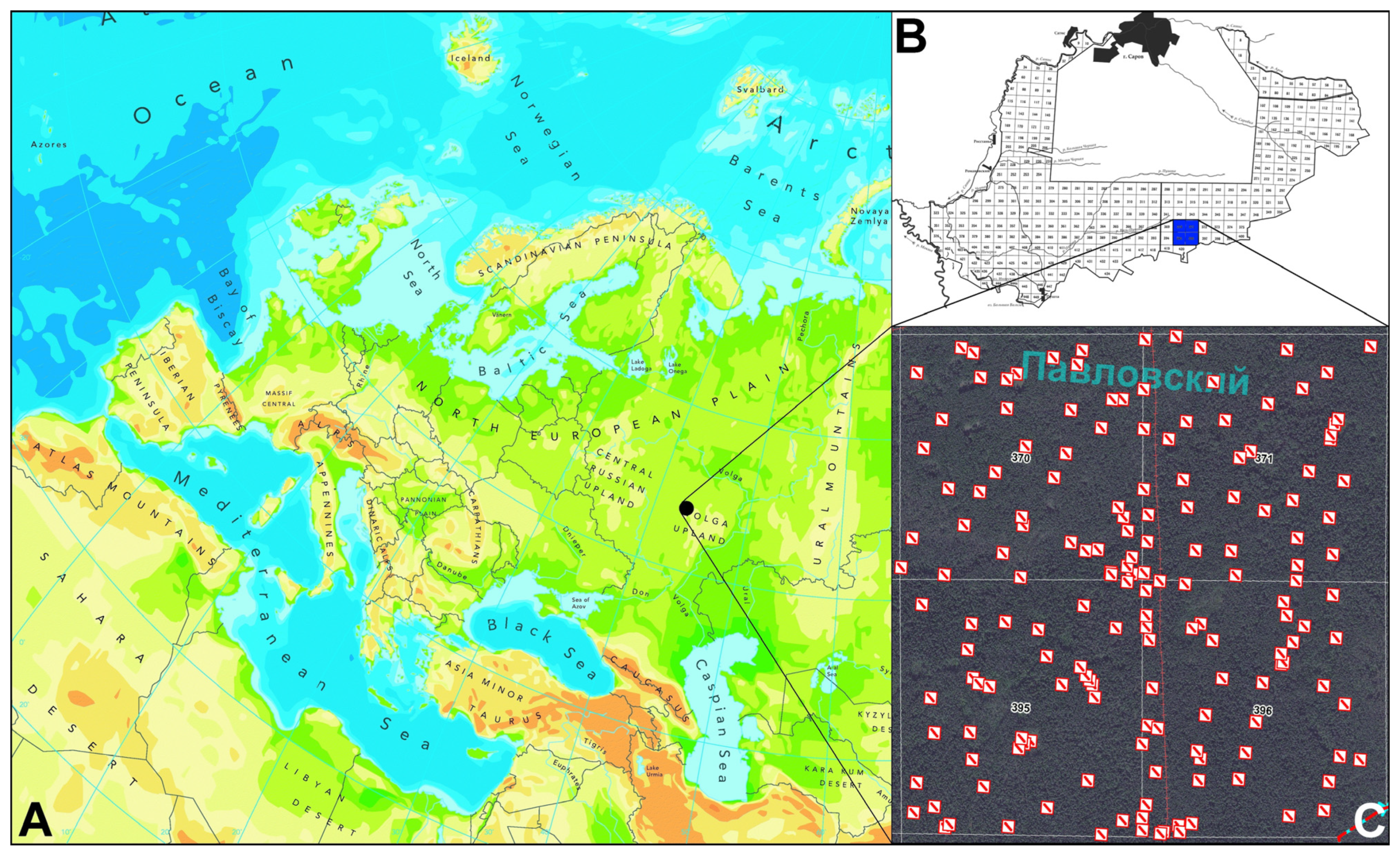
2.1. Study Area

The field surveys were conducted in the Mordovia State Nature Reserve (Figure 1). This area is located near the southern boundary of the taiga zone (54.70–54.93° N; 43.07–43.60° E; up to 190 m a.s.l.) in the centre of European Russia. Its area is 321.62 km². The soils are mainly sandy, with different podsolisation degrees [24]. The annual precipitation is 406.6–681.3 mm. The mean annual air temperature is 4.7 °C [25]. Forests cover 89.3% of the total area. Pinus sylvestris L. (hereafter—pine) is the main species forming forests. Betula pendula Roth (hereafter—birch) has the second rank in the forest-covering area. Tilia cordata Mill. (hereafter—linden) forests are situated in the north of the protected area. Quercus robur L. (hereafter—oak) forests cover small areas in the western part of the Mordovia State Nature Reserve. Picea abies (L.) H.Karst (hereafter—spruce) forests are situated mainly in floodplains of rivers and streams, covering a relatively small area [26]. Forests damaged by a wildfire in 2010 are dominated by young deciduous trees (Betula pendula and rarer Populus tremula L. and Alnus glutinosa (L.) Gaertn) [3].

2.2. Field Sampling

In this study, we selected four nearby forest compartments (numbers 370, 371, 395, 396) in the south of the Mordovia State Nature Reserve (Figure 1). The studied territory had an area of 4.61 km², selected because it represents, generally, the typical vegetation in the Mordovia State Nature Reserve, dominated mainly by pine forests. The field surveys were carried out in 2017–2020, when 161 100-m² study plots were randomly arranged (Figure 1). Among them, three plots (with the size of 2 m Ч 50 m) were established along the forest road to test whether they differed from the adjacent plots in the forest communities. Noteworthy, data from forest compartment 396 were previously partially published [20] to test the proposed approach at a small scale. Then, these data were supplemented by additional surveys, with further investigation of other (370, 371, 395) forest compartments.

In each study plot, the plant composition was investigated for conducting the analysis. Vascular plants were classified according to the Raunkiaer’s [27] life-form classification. Among bryophytes, we considered dominant terrestrial species only. The habitats were classified based on dominating plant communities as follows: coniferous forests (with at least 80% of coniferous trees in the canopy), mixed forests (mature forests, where the canopy density of either broadleaved or coniferous trees occupying at least 30%, but maximum 70%), broadleaved forests (with at least 80% of broadleaved trees in the canopy), mires, water bodies (formed in karst funnels), forest gaps (represented by cutting sites or glades existing for a long time). The number of studied plots classified to each habitat is given in

Table 1. The assignment of studied plots to each of the habitat types recognised.

Habitat	Number of Studied Plots	Proportion, %
Coniferous forests	117	72.7
Mires	20	12.4
Broadleaved forests	11	6.8
Mixed forests	7	4.3
Roads	3	1.9
Forest gaps	2	1.2
Water bodies	1	0.6

.

2.3. Data Analysis and Visualisation

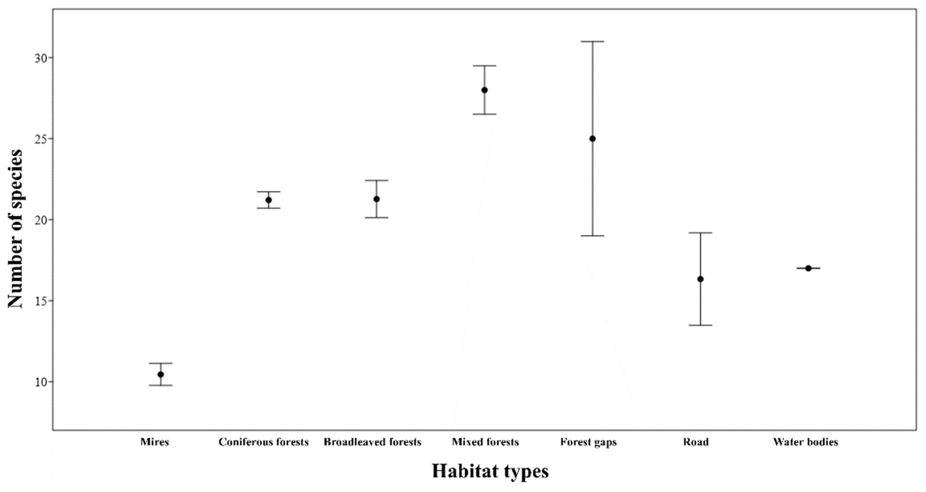
To analyse the obtained data, we, advisedly, avoided using the environmental scales of Ellenberg [17] or Landolt [18], because they were both developed in and for Central Europe. Therefore, to apply them to the Mordovia State Nature Reserve, a correction factor was needed, but it is currently absent for the study area located in Eastern Europe. To obtain the average values (measured in scale scores) of the used environmental factors for each plot, we used the Tsyganov [16] environmental scale. In contrast to the Ellenberg point scale, the Tsyganov scale demonstrates an interval (range) over which individual plant species show a predilection for environmental conditions (soil richness, light availability, soil moisture, etc.). Tsyganov [16] scale was developed in the subzone of coniferous–broadleaved forests in European Russia, where the study area was located. As mentioned above, on this scale, each factor was represented by score (gradation) values associated with survival intervals of plants. This meant that each plant species was characterised by the range of its survival, which could be identified for certain factors. In the here presented study, we used environmental factors related to the habitat illumination and soil parameters based on the Tsyganov [16] scale, namely, habitat shading (LC), moisture of soils (HD), nitrogen availability in soils (NT), pH (acidity) of soils (RC), trophicity of soils (TR) and soil moisture variability (FH). On each study plot, the average values of environmental factors were calculated as a mean of the total set of species found there. Calculations were performed using the following formula, taking into account environmental factor values of all species found in each studied plot:

$$mEFV=\frac{(x_1^{\min }+x_2^{\min }+\dots +x_n^{\min })+(x_1^{\max }+x_2^{\max }+\dots +x_n^{\max })}{2n},$$

where:

mEFV = average environmental factor value;

$x_n^{\min }$ = the minimal score value of a certain factor for n plant species;

$x_n^{\max }$ = the maximal score value of a certain factor for n plant species;

n = the number of certain plant species in the floristic list obtained in the study plot.

To encounter the probable indicator plant species based on the Tsyganov [16] scale, we checked the total number of plant species found in the study area. Then, we found taxa with the narrowest score intervals between maximal and minimal values of environmental factors [16] (pp. 135–184). One more criterion was the 5% frequency of occurrence. Taking into account that 161 plots were analysed, such species had to have been found on at least eight study plots. As a result, we chose Eriophorum vaginatum L., typical for habitats extremely poor in nutrients. Among plants of broadleaved forests, we selected Pulmonaria obscura Dumort., typical for broadleaved forests rich in nutrients [28]. Their locations were compared with the distribution of the environment factor gradients in the study area.

To visualise the distribution of gradients of the used environmental factors, we used relevant contour maps applied as background images in the software “Surfer” v. 11 [29]. We interpolated contour maps using the method of kriging through the default linear variogram. We used obtained average values of environmental factors as variable Z. Concerning the four selected environmental factors (habitat shading, moisture of soils, nitrogen availability of soils and soil acidity (pH)), contour maps were overlapped using a 70% opacity. To highlight the most extreme (black vs. white) areas, we increased the picture contrast by 50% with a decrease in brightness by 50%.

We performed a statistical analysis using MS Excel 2007 (Redmond, WA: Microsoft Press, Chicago, IL, USA) and PAST 4.07 [30]. The principal component analysis (PCA) was used to reveal the major environmental factors influencing the spatial arrangement of the study plots. For the interpretation, average values (in scores) of these factors on the established plots were plotted onto a PCA ordination diagram as supplementary environmental data. A one-way permutational multivariate analysis of variance (PERMANOVA) was applied to test the differences in environmental conditions among the distinguished habitat types based on values of Tsyganov [16]. We tested its significance based on 9999 unrestricted permutations of raw data.

3. Results

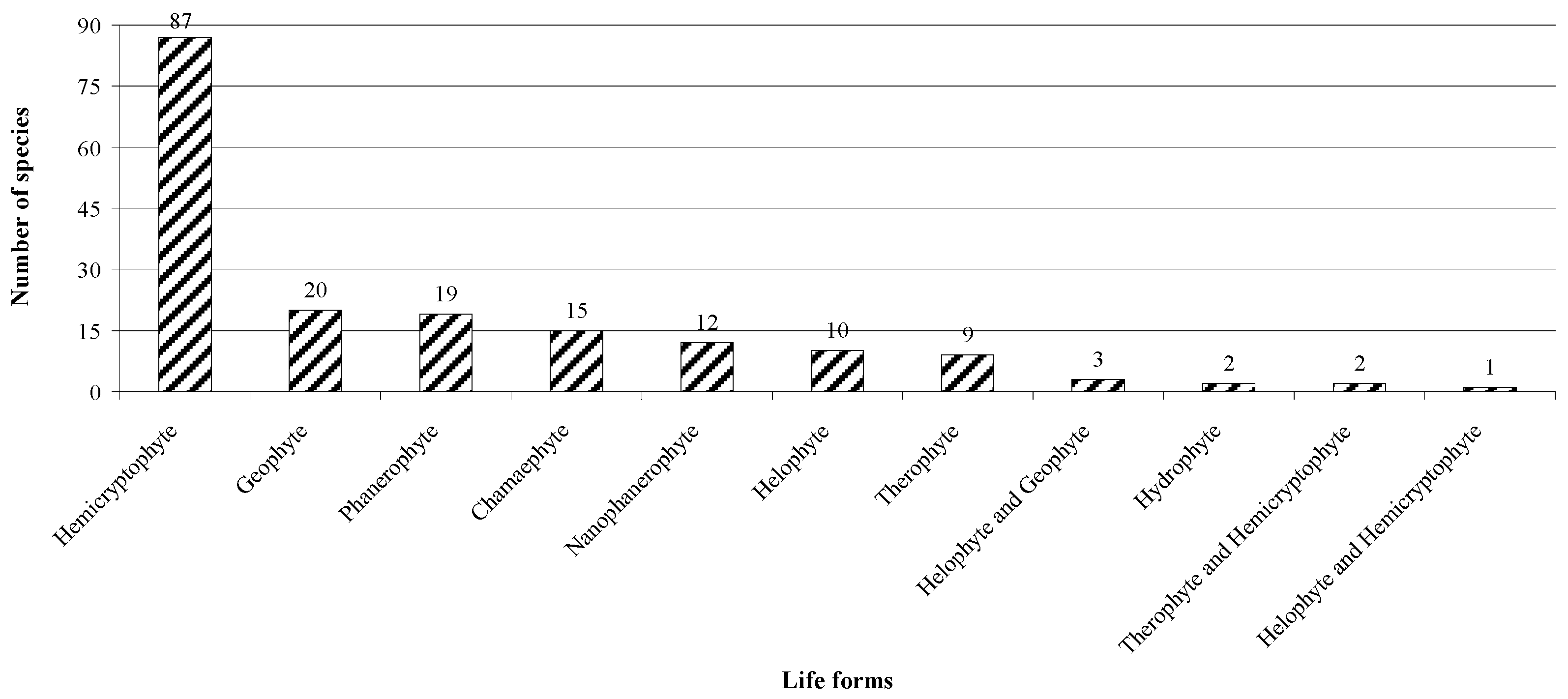
3.1. Vascular Plant Flora of the Study Area

During 2017–2020, we registered 180 vascular plant species, belonging to 128 genera and 53 families, on the 161 study plots arranged regularly in four forest compartments of the Mordovia State Nature Reserve, European Russia (Table S1 in Supplementary Materials). The families richest in species were Poaceae (19 species, which meant 10.6% of the whole flora), Cyperaceae (18 species; 10.0%), Asteraceae (15 species; 8.3%), Rosaceae (12 species; 6.7%) and Ericaceae (10 species; 5.6%). The biomorphological analysis of the vascular plant flora according to the Raunkiaer [27] classification demonstrated the predominance of hemicryptophytes (87 species) and, in a lesser degree of geophytes (20 species), representing the herb layer in the studied forest communities (Figure 2). A considerable number of plants species was presented by phanerophytes (19 species) and nanophanerophytes (12 species), forming, respectively, the canopy layer and understory layer in the forest communities of the Mordovia State Nature Reserve.

We evaluated the number of plant species in the specified habitat types. Figure 3 shows that the lowest number of species was found in mires (10.5 ± 0.7 species), followed by forest roads (16.3 ± 2.8 species) and a single water body (17 species). Intermediate positions had both pure coniferous (21.2 ± 10.5 species) and pure broadleaved (21.3 ± 1.1 species) forests. By combining the properties of both above-mentioned forest types, mixed forests were characterised by the highest (28.0 ± 1.5 species) number of species. A similar value of taxonomic richness (25.0 ± 6.0 species) was found in forest gaps, where features of both forests and open habitats (such as grasslands) were combined.

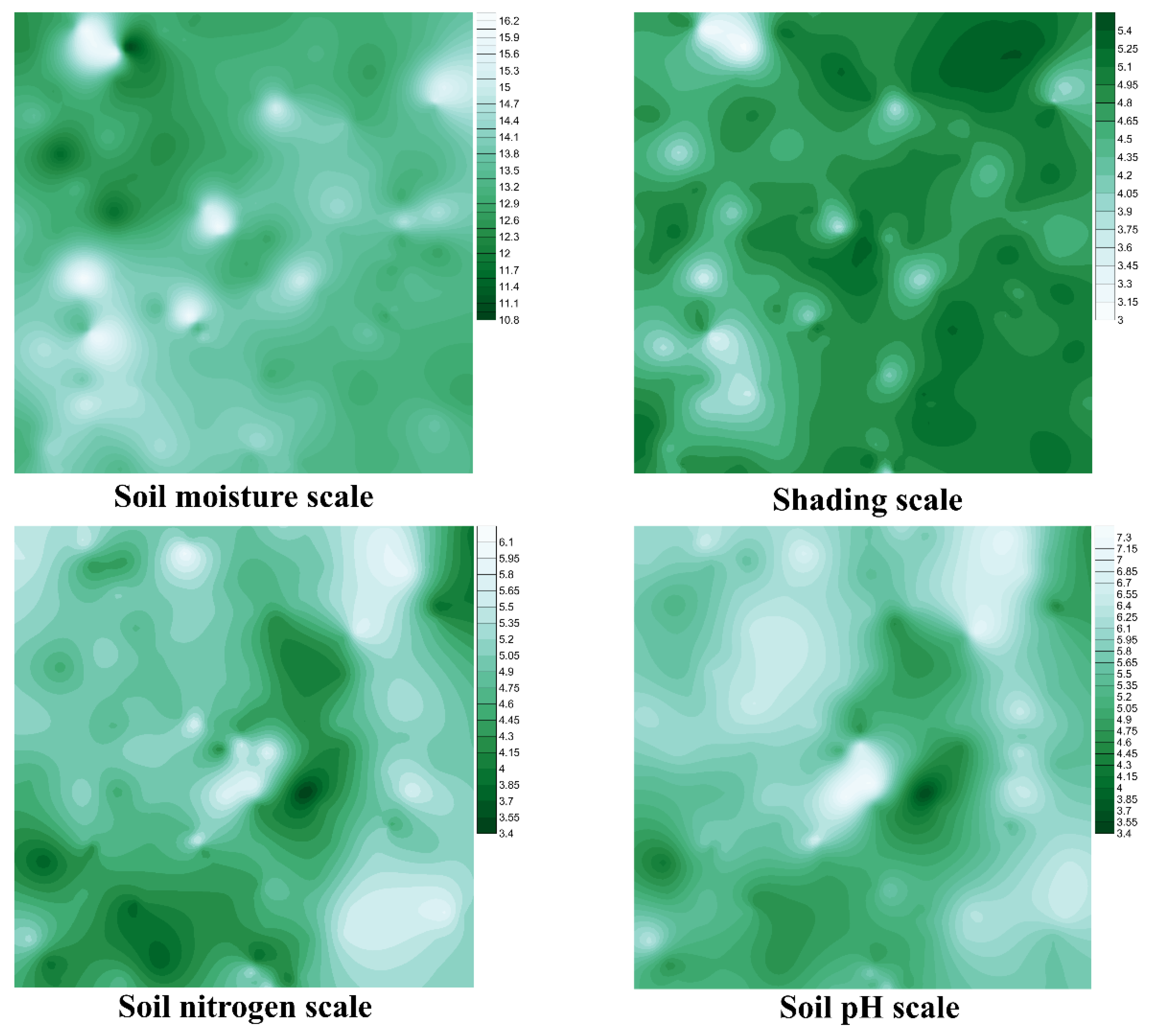
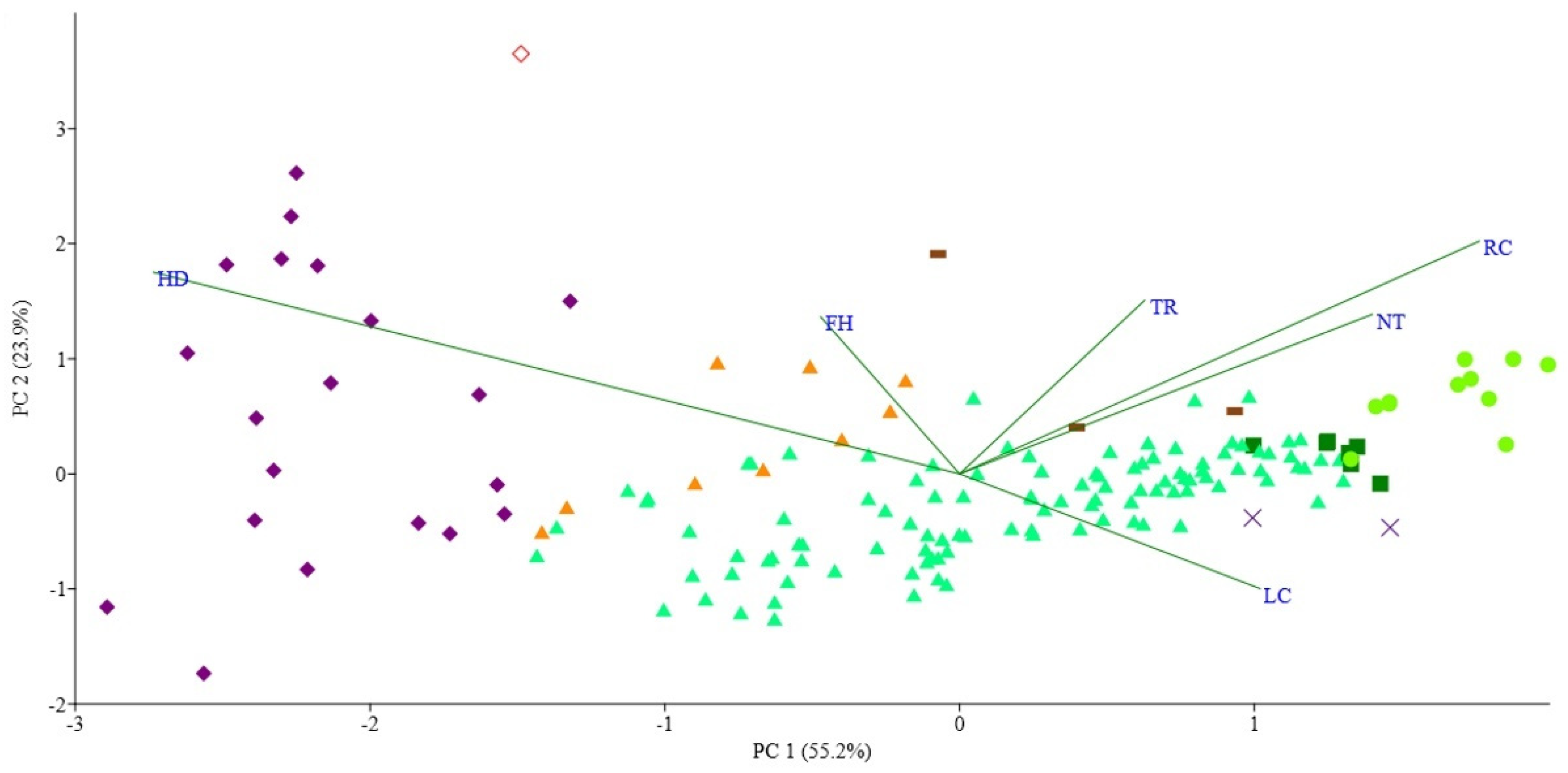
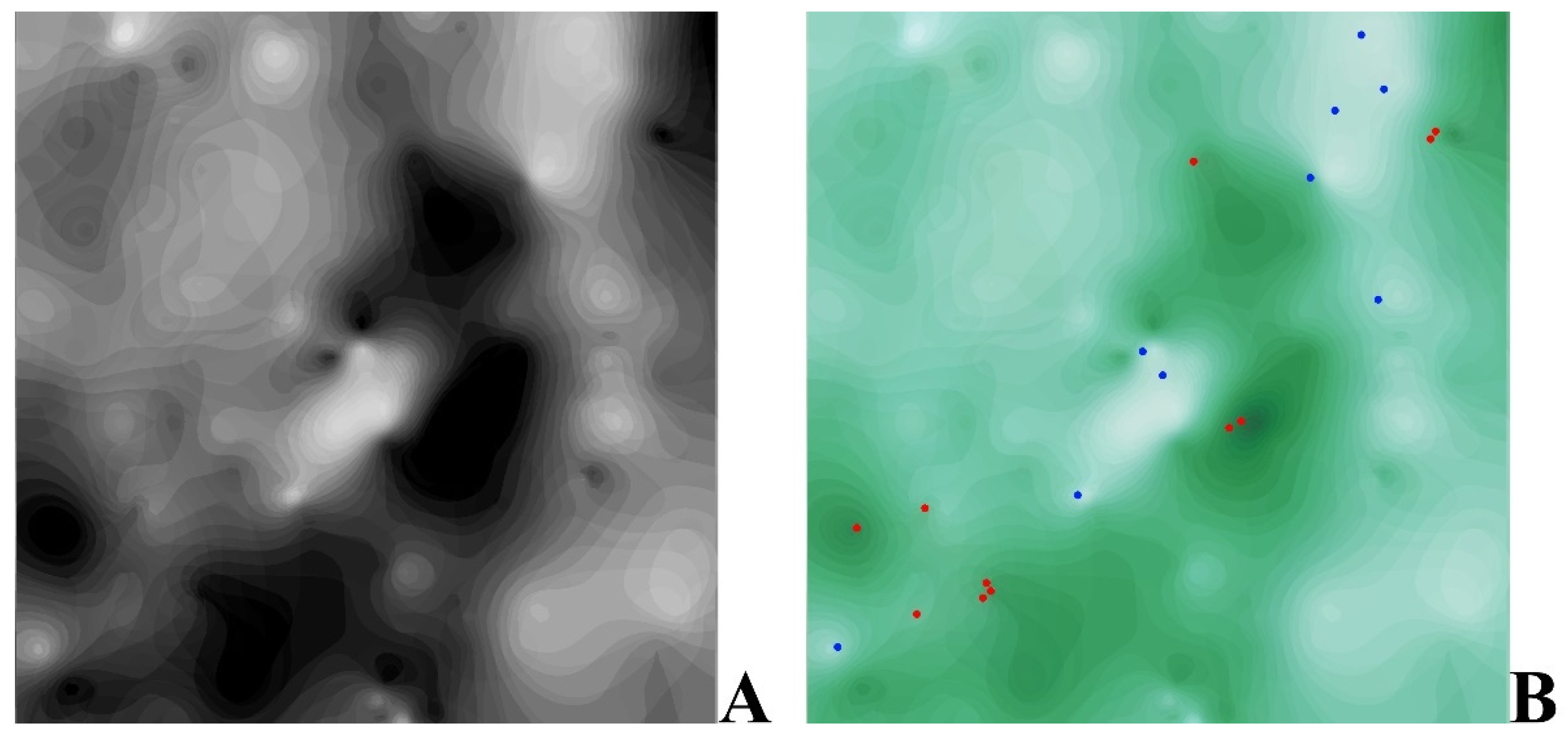
3.2. Plant-Environment Relationships Based on the Tsyganov Scale

For testing our assignment of study plots to habitat types, the principal component analysis was conducted based on values of six environmental factors according to Tsyganov [16]. All study plots were arranged in accordance with values of the used environmental factors (Figure 4). It was obvious that the soil moisture had a considerable influence on the arrangement of study plots. Mires and the only water body were most distinguished from the other habitats. We could see the transition from the most moisturised mires on poor soils to spruce–pine and pine forests, then to mixed forests and, finally, to the shadiest broadleaved forests on the richest soils. The three “road”-classified study plots were, generally, located near the group of coniferous forests. This was caused by the road’s location within the pine forest massif in the study area, while the presence of some weeds and meadow plants (Table S1 in Supplementary Material) slightly distinguished this group from coniferous forest plots. Consisting of both nemoral and boreal plant species (Table S1 in Supplementary Material), mixed forests represented a transitional group between coniferous and broadleaved forests in Figure 4. On the other hand, broadleaved forests were relatively well-distinguished, as they were the shadiest plant communities on the richest soils with high values of both pH and nitrogen amounts. Forest gaps were also well-separated due to a higher illumination than adjacent coniferous and mixed forests.

PERMANOVA confirmed the relatively correct distinguishing of habitat types. The analysis demonstrated significant (p < 0.050) differences based on six selected Tsyganov [16] environment factors (Figure 4). Exceptions were such pairs as: water bodies—forest gaps (p = 0.329); water bodies—mixed forests (p = 0.123); water bodies—broadleaved forests (p = 0.084); water bodies—roads (p = 0.254); forest gaps—roads (p = 0.096).

Based on the calculated average values of environmental factors obtained for each study plot, we prepared gradient maps of the four environmental factors (Figure 5). They showed variations in the gradients of the mean environmental factor values through the study area (Figure 5). We could see more or less illuminated and/or wet areas that corresponded to differences in habitat conditions and, accordingly, the composition of plant species.

We combined the four maps showing the spatial distribution of the used environmental factor gradients. Hence, areas of the greatest overlap of all obtained maps were produced (Figure 6A). The consequent treatment (see Material and Methods) had highlighted areas with certainly extreme (pure white vs. pure black colours) conditions. Then, we added the locations of the selected plants (Eriophorum vaginatum vs. Pulmonaria obscura) to the untreated map (Figure 6B).

Figure 6B shows that blue dots (Pulmonaria obscura locations) were confined to white and light green areas. These sites were covered by the shadiest plant communities placed on the richest soils with a lower moisture amount. These areas referred, mainly, to broadleaved or rarer mixed forests. On the other hand, red dots (Eriophorum vaginatum locations) were confined to dark green areas (Figure 6B). These sites were characterised by the highest habitat illumination, as well as most acidic and moisturised soils with the lowest amount of available nitrogen. These areas referred to Sphagnum mires.

4. Discussion

Although the studied territory was situated at the boundary of forest-steppe and forest zones, the analysis of the vascular plant flora demonstrated its boreal features reflected in the high position of Cyperaceae and Ericaceae in the spectrum of families. In contrast to the floras of many administrative regions in the River Volga basin in European Russia [31], the flora of the study area was similar to the taiga flora type [32,33]. This coincided with the results of the biomorphological analysis, which demonstrated a high predominance of hemicryptophytes with high proportions of phanerophytes, nanophanerophytes and chamaephytes. Our results coincided with similar studies conducted in boreal regions of Europe [33,34].

The classification of study plots according to habitat types demonstrated a clear separation of mires in terms of the species number. Such a low species richness is typical for Sphagnum mires [35], while these habitats are important “islands” for some threatened species [36,37]. Therefore, the discovery and conservation of these habitats are crucial to protect populations of threatened species, many of which are specialists. The only water body had a species composition of aquatic and peatland plants. Therefore, the species richness was considerably higher than in mires. However, the vegetation succession of karst funnels seemed to lead to a mire formation in the future [38]. In contrary to the two previous habitat types, forest communities, mainly, consisted of generalists. These habitats were represented by the highest species richness in the studied territory (Figure 3). This finding coincided with [39,40], demonstrating a higher species richness of mixed forests in comparison with pure coniferous or deciduous forests. Despite the small sampling size of the forest gap type, the average species richness was relatively high. We assumed that the increase in the sampling size would decrease the standard deviation value (Figure 3) with the same high species richness. Our assumption was based on the knowledge that forest gaps are characterised by a higher species richness due to the combination of both light-adapted and shade-tolerant plants [41]. The road habitat type was characterised by a decrease in species number in comparison with adjacent forest communities due to an anthropogenic load. It resulted in the appearance of some light-adapted species, such as Achillea millefolium L. and Plantago major L. Despite of this fact, differences in species composition in these sites did not considerably influence the environmental conditions of habitats [20].

These floristic results coincided with results of the principal component analysis based on Tsyganov’s [16] environmental factors. The spatial distribution of study plots along gradients of three factors (habitat shading, moisture of soils and nitrogen availability of soils) was in agreement with the results of other studies [13,20,21]. Although the habitat types seemed to be clearly distinguished in Figure 4, PERMANOVA did not allow us to conclude on the correct separation of water bodies, forest gaps and roads. However, the only water body included in the study was far separated from the other study plots in Figure 4. Based on our experience and some methodological studies [42,43], we assumed that the insignificance of differences with other habitat types was based on the small sampling size of the above-mentioned habitat types. Due to the well-fitted sampling of broadleaved forests in our study, we guessed that each group should be represented by at least 3–4% of the entire number of samples (here, study plots) in the dataset. Our assumption could be proved as a result of a further increase in the number of study plots classified as forest gaps, water bodies and forest roads.

The obtained contour maps of gradients of the four studied environmental factors showed remarkable similarities. In general, the values of all environmental factors changed simultaneously through the study area. Such co-ordinated changes in environmental conditions were expressed in the formation of clearly delineated plant communities (habitat types) [44]. However, the highest probability of plant location identification was characterised for habitats with environmental conditions atypical for the study area. In our research, such habitats were broadleaved forests and mires, which was confirmed by their distinct position in Figure 4. Therefore, based on the combined counter maps (Figure 6A), we could conditionally identify areas where Pulmonaria obscura and Eriophorum vaginatum could be discovered. In this connection, even if Pulmonaria obscura had not been found in other suitable areas (such as white and light green areas in the upper left part of Figure 6B), this would not mean that P. obscura was absent there. This species could have either just been overlooked during the investigation or did not yet penetrate these areas. This was correct too for other plant species that allowed us to provide prospects for the further monitoring of certain plant distributions in suitable areas.

However, based on the applied approach, we could not find areas suitable for casual plant species (e.g., weeds or alien plants), if they did not form weed-dominated plant communities. In intact or almost undisturbed habitats, the weed presence could be determined only by using floristic surveys. Under such conditions, this approach was suitable for species specialists growing in habitats with specific environmental conditions (e.g., aquatic habitats, oligotrophic wetlands).

5. Conclusions

The obtained results of floristic surveys allowed us to determine environmental conditions in the study area at the southern border of the taiga zone, European Russia. Based on the environmental scales of Tsyganov [16], the spatial distribution of only plant specialists could be recognised well, being indicators of environmental conditions. The allocation of plant generalists was impossible based on this approach. The correctness of the habitat distinguishing based on dominated plant species was well-testable using environmental conditions revealed for these sites. However, a too small sampling size per habitat did not allow us to determine clear conclusions. Each group should be represented by at least 3–4% samples of the whole sampling set.

The development of a detailed contour map of environmental factors for the entire protected area would allow (i) to obtain complete data on the distribution of plant species in the Mordovia State Nature Reserve, (ii) to build distribution maps of environment factor gradients of the protected area and (iii) to, finally, compose conclusions on possible locations of plant species specialists in the Mordovia State Nature Reserve. We also proposed the use of the applied approach in plant ecology studies in the subzone of coniferous–deciduous forests of Eastern Europe.

References

1. Pottier, J.; Dubuis, A.; Pellissier, L.; Maiorano, L.; Rossier, L.; Randin, C.F.; Vittoz, P.; Guisan, A. Climate and species assembly predictions. Glob. Ecol. Biogeogr. 2013, 22, 52–63. [Google Scholar] [CrossRef]
2. John, R.; Dalling, J.W.; Harms, K.E.; Yavitt, J.B.; Stallard, R.F.; Mirabello, M.; Hubbell, S.P.; Valencia, R.; Navarrete, H.; Vallejo, M.; et al. Soil nutrients influence spatial distributions of tropical tree species. Proc. Natl. Acad. Sci. USA 2007, 104, 864–869. [Google Scholar] [CrossRef] [Green Version]
3. Khapugin, A.A.; Vargot, E.V.; Chugunov, G.G. Vegetation recovery in fire-damaged forests: A case study at the southern boundary of the taiga zone. For. Stud. 2016, 64, 39–50. [Google Scholar] [CrossRef] [Green Version]
4. Lennon, J.J.; Beale, C.M.; Reid, C.L.; Kent, M.; Pakeman, R.J. Are richness patterns of common and rare species equally well explained by environmental variables? Ecography 2011, 34, 529–539. [Google Scholar] [CrossRef]
5. Popov, S.Y.; Makukha, Y.A. Distribution patterns of Ptilium crista-castrensis (Bryophyta, Hypnaceae) in the East European Plain and Eastern Fennoscandia. Nat. Conserv. Res. 2019, 4, 93–98. [Google Scholar] [CrossRef]
6. Dubuis, A.; Rossier, L.; Pottier, J.; Pellissier, L.; Vittoz, P.; Guisan, A. Predicting current and future spatial community patterns of plant functional traits. Ecography 2013, 36, 1158–1168. [Google Scholar] [CrossRef]
7. Gebremedihin, K.M.; Birhane, E.; Tadesse, T.; Gbrewahid, H. Restoration of degraded drylands through exclosures enhancing woody species diversity and soil nutrients in the highlands of Tigray, Northern Ethiopia. Nat. Conserv. Res. 2018, 3, 1–20. [Google Scholar] [CrossRef]
8. Khan, W.; Khan, S.M.; Ahmad, H.; Ahmad, Z.; Page, S. Vegetation mapping and multivariate approach to indicator species of a forest ecosystem: A case study from the Thandiani sub Forests Division (TsFD) in the Western Himalayas. Ecol. Indic. 2016, 71, 336–351. [Google Scholar] [CrossRef]
9. Pajunen, A.M.; Kaarlejärvi, E.M.; Forbes, B.C.; Virtanen, R. Compositional differentiation, vegetation-environment relationships and classification of willow-characterized vegetation in the western Eurasian Arctic. J. Veg. Sci. 2010, 21, 107–119. [Google Scholar] [CrossRef]
10. Jarema, S.I.; Samson, J.; McGill, B.J.; Humphries, M.M. Variation in abundance across a species’ range predicts climate change responses in the range interior will exceed those at the edge: A case study with North American beaver. Glob. Chang. Biol. 2009, 15, 508–522. [Google Scholar] [CrossRef]
11. Cui, B.S.; Zhai, H.J.; Dong, S.K.; Chen, B.; Liu, S.L. Multivariate analysis of the effects of edaphic and topographical factors on plant distribution in the Yilong lake basin of Yun-Gui Plateau, China. Can. J. Plant. Sci. 2009, 89, 209–219. [Google Scholar] [CrossRef]
12. Potts, M.D.; Ashton, P.S.; Kaufman, L.S.; Plotkin, J.B. Habitat patterns in tropical rain forests: A comparison of 105 plots in northwest Borneo. Ecology 2002, 83, 2782–2797. [Google Scholar] [CrossRef]
13. Seregin, A.P. Further east: Eutrophication as a major threat to the flora of Vladimir Oblast, Russia. Environ. Sci. Pollut. Res. 2014, 21, 12883–12897. [Google Scholar] [CrossRef] [PubMed]
14. Smirnova, O.V.; Lugovaya, D.V.; Prokazina, T.S. Model Reconstruction of Restored Taiga Forest Cover. Biol. Bull. Rev. 2013, 3, 493–504. [Google Scholar] [CrossRef]
15. Ramenskiy, L.G.; Tsatsenkin, I.A.; Chijikov, O.N.; Antipin, N.A. Ecological Evaluation of Natural Grasslands by the Use of Vegetation Cover; Selkhozgiz: Moscow, Russia, 1956. (In Russian) [Google Scholar]
16. Tsyganov, D.N. Phytoindication of Ecological Regimes in the Mixed Coniferous-Broad-Leaved Forest Subzone; Nauka: Moscow, Russia, 1983. (In Russian) [Google Scholar]
17. Ellenberg, H.; Weber, H.E.; Düll, R.; Wirth, V.; Werner, W. Zeigerwerte von Pflanzen in Mitteleuropa, 3, durch gesehene Aufl. Scr. Geobot. 2001, 18, 1–261. [Google Scholar]
18. Landolt, E.; Bäumler, B.; Erhardt, A.; Hegg, O.; Klötzli, F.; Lämmler, W.; Nobis, M.; Rudmann-Maurer, K.; Schweingruber, F.H.; Theurillat, J.P.; et al. Ecological Indicator Values and Biological Attributes of the Flora of Switzerland and the Alps; Haupt: Bern, Switzerland, 2010. [Google Scholar]
19. Didukh, Y.P. The Ecological Scales for the Species of Ukrainian Flora and Their Use in Synphytoindication; Phytosociocentre: Kyiv, Ukraine, 2011. [Google Scholar]
20. Khapugin, A.A. Benefits from visualization of environmental factor gradients: A case study in a protected area in central Russia. Rev. Chapingo Ser. Cienc. For. Y Del Ambient. 2019, 25, 383–398. [Google Scholar] [CrossRef]
21. Priputina, I.; Zubkova, E.; Shanin, V.; Smirnov, V.; Komarov, A. Evidence of plant biodiversity changes as a result of nitrogen deposition in permanent pine forest plots in central Russia. Ecoscience 2014, 21, 286–300. [Google Scholar] [CrossRef]
22. Gusev, A.P. Specific features of early stages of progressive succession in an anthropogenic landscape: An example from southeastern Belarus. Russ. J. Ecol. 2009, 40, 160–165. [Google Scholar] [CrossRef]
23. Khapugin, A.A. Hieracium sylvularum (Asteraceae) in the Mordovia State Nature Reserve: Invasive plant or historical heritage of the flora? Nat. Conserv. Res. 2017, 2, 40–52. [Google Scholar] [CrossRef] [Green Version]
24. Kuznetsov, N.I. The conditions of existence and main features of the vegetation cover structure on the territory of Mordovia State Reserve. 1939 year. Proc. Mordovia State Nat. Reserve 2014, 12, 79–195. (In Russian) [Google Scholar]
25. Bayanov, N.G. Climate changes of the northwest of Mordovia during the period of existence of the Mordovia Reserve according to the meteorological observations in Temnikov. Proc. Mordovia State Nat. Reserve 2015, 14, 212–219. [Google Scholar]
26. Tereshkin, I.S.; Tereshkina, L.V. Vegetation of the Mordovia Reserve. Successive series of the successions. Proc. Mordovia State Nat. Reserve 2006, 7, 186–287. (In Russian) [Google Scholar]
27. Raunkiaer, C. The Life Forms of Plant and Statistical Plant Geography; Clarendon Press: Oxford, UK, 1934. [Google Scholar]
28. Marinšek, A.; Čarni, A.; Šilc, U.; Manthey, M. What makes a plant species specialist in mixed broad-leaved deciduous forests? Plant Ecol. 2015, 216, 1469–1479. [Google Scholar] [CrossRef]
29. Golden Software Inc. Surfer Mapping System. v. 11.1.719 Software. USA, 2012. Available online: http://www.goldensoftware.com/products/surfer/ (accessed on 1 August 2021).
30. Hammer, Ø.; Harper, D.A.T.; Ryan, P.D. PAST: Paleontological statistics software package for education and data analysis. Palaeontol. Electron. 2001, 4, 9. [Google Scholar]
31. Ivanova, A.V.; Kostina, N.V.; Rozenberg, G.S.; Saksonov, S.V. Family ranges of the flora of the Volga River Basin territory. Bot. Zhurnal 2016, 101, 1042–1055. (In Russian) [Google Scholar]
32. Khokhryakov, A.P. Taxonomic spectra and their role in comparative floristics. Bot. Zhurnal 2000, 85, 1–11. (In Russian) [Google Scholar]
33. Talbot, S.S.; Talbot, S.L.; Schofield, W.B. Vascular flora of Izembek National Wildlife Refuge, Westernmost Alaska Peninsula, Alaska. Rhodora 2006, 108, 249–293. [Google Scholar] [CrossRef]
34. Demina, G.V.; Zakirov, A.R. Floristic characterization of the territory adjacent to the “Gray Heron Colony” protected area. EurAsian J. BioSci. 2018, 12, 227–231. [Google Scholar]
35. Ingerpuu, N.; Vellak, K.; Kukk, T.; Pärtel, M. Bryophyte and vascular plant species richness in boreo-nemoral moist forests and mires. Biodivers. Conserv. 2001, 10, 2153–2166. [Google Scholar] [CrossRef]
36. Hájek, M.; Hájková, P.; Apostolova, I.; Horsák, M.; Plášek, V.; Shaw, B.; Lazarova, M. Disjunct Occurrences of Plant Species in the Refugial Mires of Bulgaria. Folia Geobot. 2009, 44, 365–386. [Google Scholar] [CrossRef]
37. Khapugin, A.A.; Ruchin, A.B. Red Data Book vascular plants in the Mordovia State Nature Reserve, a Protected Area in European Russia. Wulfenia 2019, 26, 53–71. [Google Scholar]
38. Mazei, Y.A.; Tsyganov, A.N.; Bobrovsky, M.V.; Mazei, N.G.; Kupriyanov, D.A.; Gałka, M.; Rostanets, D.V.; Khazanova, K.P.; Stoiko, T.G.; Pastukhova, Y.A.; et al. Peatland Development, Vegetation History, Climate Change and Human Activity in the Valdai Uplands (Central European Russia) during the Holocene: A Multi-Proxy Palaeoecological Study. Diversity 2020, 12, 462. [Google Scholar] [CrossRef]
39. Jobidon, R.; Cyr, G.; Thiffault, N. Plant species diversity and composition along an experimental gradient of northern hardwood abundance in Picea mariana plantations. For. Ecol. Manag. 2004, 198, 209–221. [Google Scholar] [CrossRef]
40. Barbier, S.; Gosselin, F.; Balandier, P. Influence of tree species on understory vegetation diversity and mechanisms involved—A critical review for temperate and boreal forests. For. Ecol. Manag. 2008, 254, 1–15. [Google Scholar] [CrossRef]
41. Hammond, M.E.; Pokorny, R.; Dobrovolný, L.; Friedl, M.; Hiitola, N. Effect of gap size on tree species diversity of natural regeneration–case study from Masaryk training forest school enterprise Křtiny. J. For. Sci. 2020, 66, 1–14. [Google Scholar] [CrossRef]
42. Hackshaw, A. Small studies: Strengths and limitations. Eur. Respir. J. 2008, 32, 1141–1143. [Google Scholar] [CrossRef]
43. Ajay, S.; Micah, B. Sampling techniques and determination of sample size in applied statistics research: An overview. Int. J. Econ. Commer. Manag. 2014, 2, 1–22. [Google Scholar]
44. Vahdati, F.B.; Mehrvarz, S.S.; Dey, D.C.; Naqinezhad, A. Environmental factors–ecological species group relationships in the Surash lowland-mountain forests in northern Iran. Nord. J. Bot. 2017, 35, 240–250. [Google Scholar] [CrossRef]
Figure 1. The position of 161 study plots in Europe (A), in the Mordovia State Nature Reserve (B) and the studied forest compartments (C). (Source of the modified map of Europe: http://www.eea.europa.eu/legal/copyright (accessed on 15 August 2021)).
Forests 12 01475 g001
Figure 2. Groups of life forms of plant species classified according to Raunkiaer [27].
Forests 12 01475 g002
Figure 3. The mean number (whiskers show standard error) of plant species per habitat type in the study area (Mordovia State Nature Reserve, European Russia).
Forests 12 01475 g003
Figure 4. Ordination diagram of the principal component analysis (PCA) of study plots in the Mordovia State Nature Reserve, European Russia. Symbols: purple diamonds—mires; red empty diamonds—water bodies; triangles—coniferous forests (orange—spruce–pine forests; green—pine forests); green squares—mixed forests; green dots—broadleaved forests; dashes—roads; ×—Forest gaps. Environmental factors: LC = habitat shading; HD—moisture of soils; NT—nitrogen availability of soils; RC—acidity (pH) of soils; TR—trophicity of soils; FH—soil moisture variability. To obtain environmental gradients, average values of environmental factors were plotted onto the principal component analysis ordination diagram as supplementary environmental variables.
Forests 12 01475 g004
Figure 5. Interpolated maps of the spatial gradient distribution of the four environmental factors. Score scales at the right side of each map show values of environmental factors according to Tsyganov’s [16] environmental scales.
Forests 12 01475 g005
Figure 6. The four combined maps showing the spatial distribution of average environmental factor values (A) and the same in combination with locations of Eriophorum vaginatum (red dots) and Pulmonaria obscura (blue dots) in the selected forest compartments (B).
Forests 12 01475 g006