Unmanned Aerial System and Machine Learning Techniques Help to Detect Dead Woody Components in a Tropical Dry Forest


Abstract
1. Introduction
2. Materials and Methods
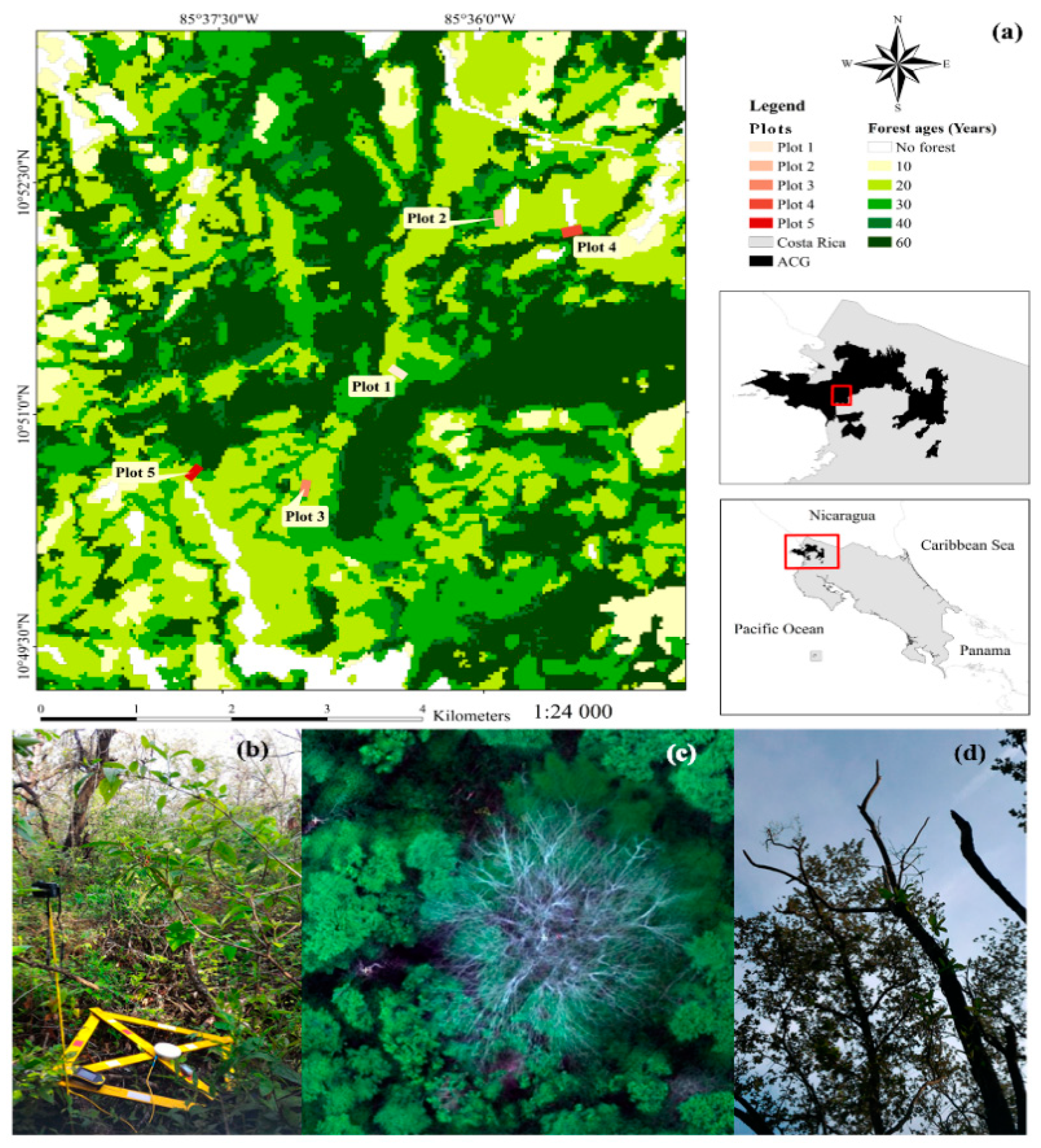
2.1. Study Site
2.2. Field Acquisition
2.3. Data Preprocessing
2.3.1. Radiometric Correction and Mosaicking
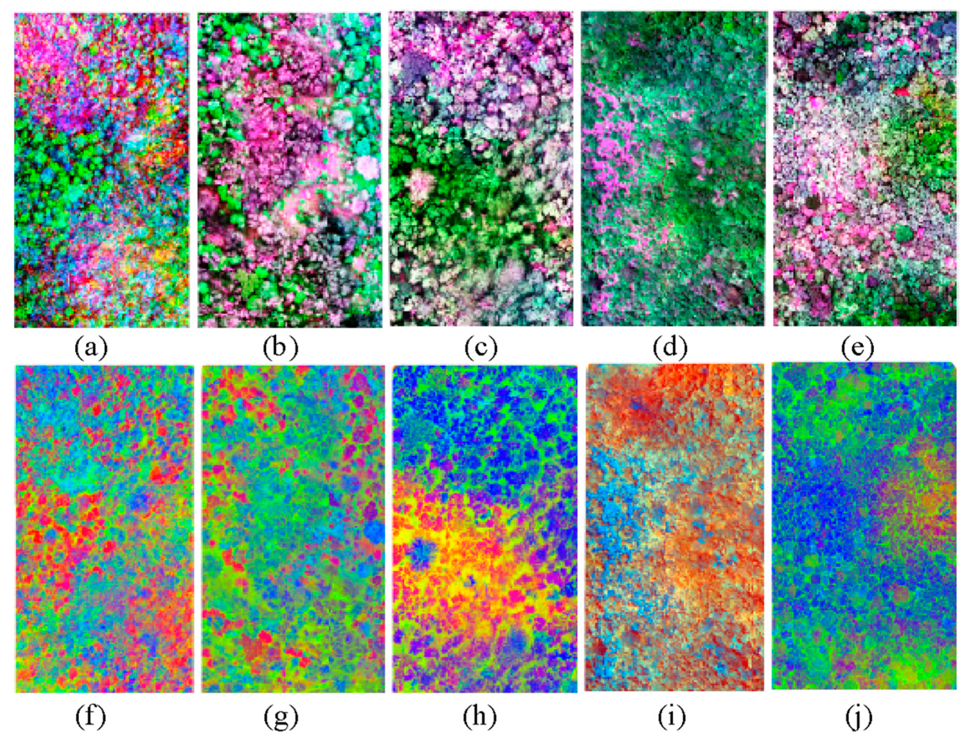
2.3.2. Data Reduction and Transformation
2.4. Classification Models
2.5. Creation of Training and Validation Datasets
2.6. Implementation of Classification Models
2.7. Model Validation
2.8. Differences in the Spatial Coverage of the Dead Woody Components between Plots
3. Results
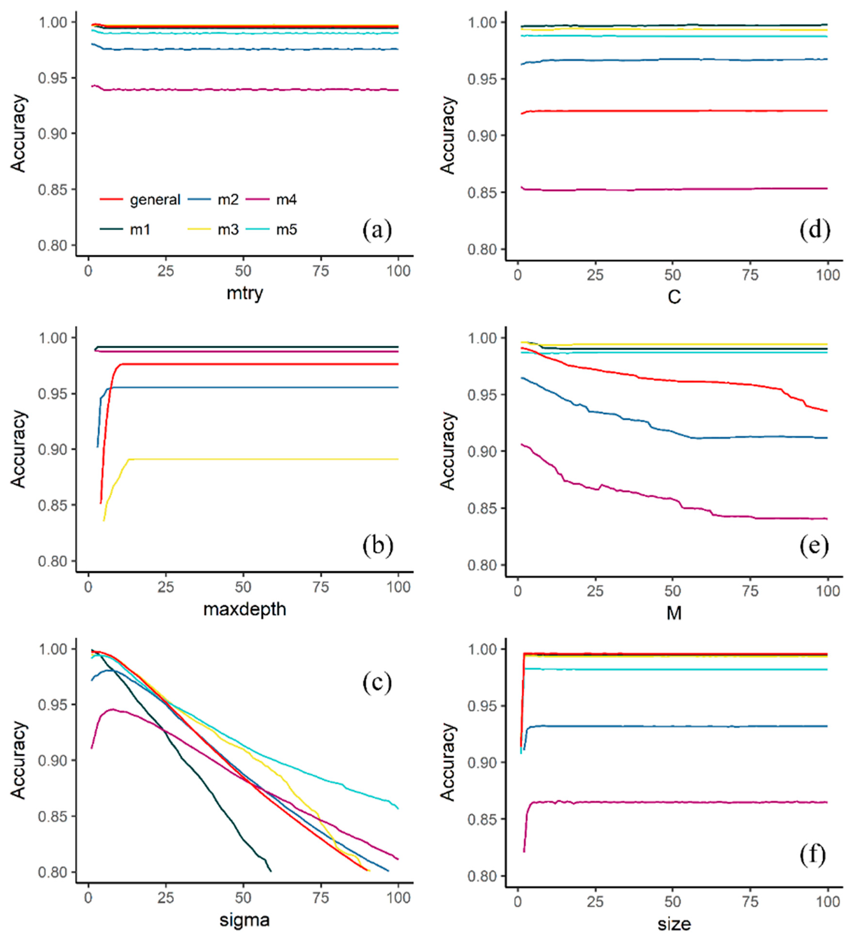
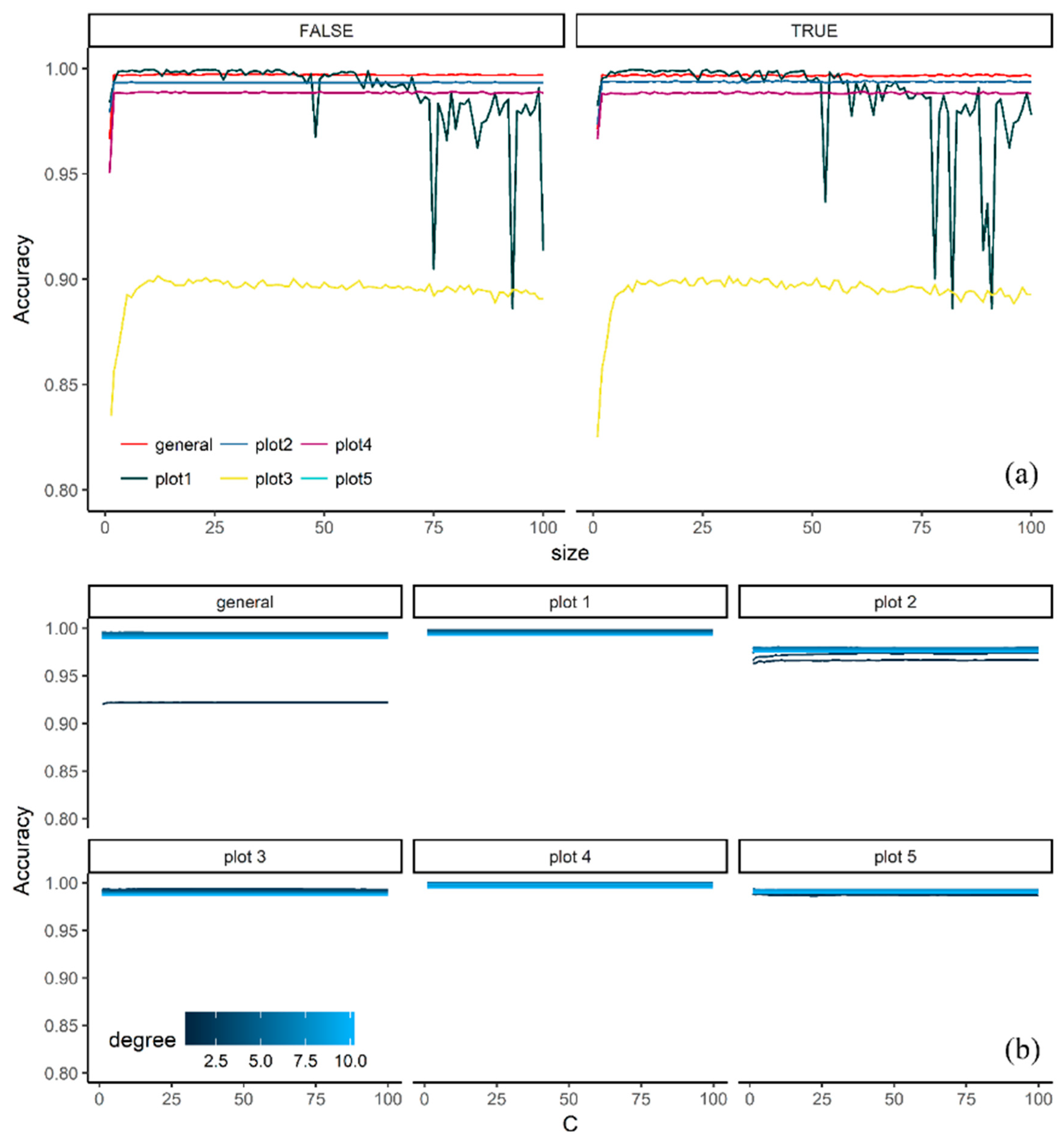
3.1. Effect of Tuning Parameters on the Accuracy Values
3.2. Model Selection
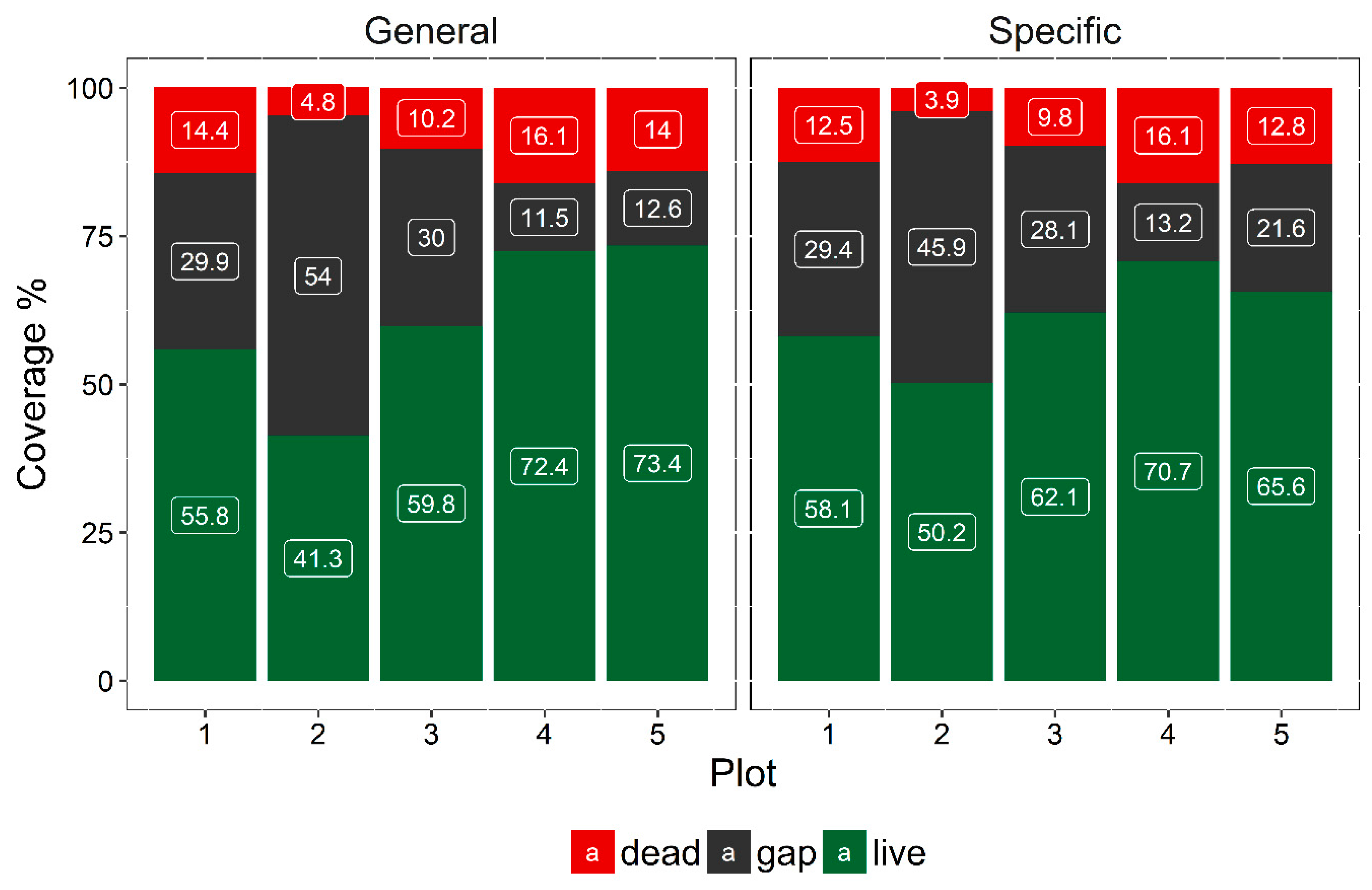
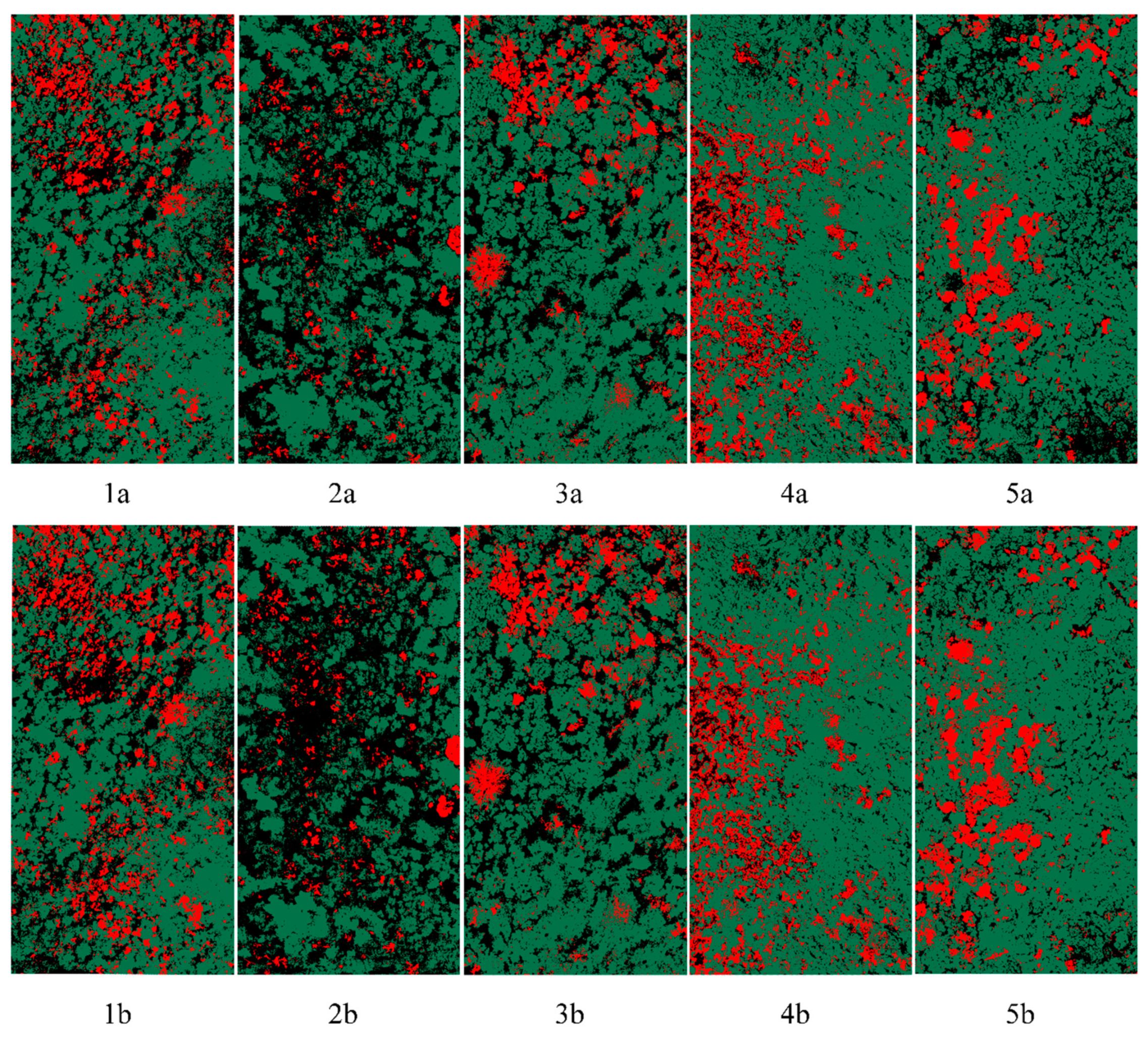
3.3. Extent of Dead Woody Components
4. Discussion
4.1. Effect of Tuning Parameters on the Accuracy Values and Performance of Selected Models
4.2. Extension of Dead Woody Components
4.3. Dead Woody Components and Their Ecological Implications
4.4. The Influence of Enviromental Conditions and Time in Accuracy of Remotely Sensed Data at Tropical Dry Forests
5. Conclusions
Author Contributions
Funding
Acknowledgments
Conflicts of Interest
References
- Masson-Delmotte, V.; Zhai, P.; Pörtner, H.-O.; Roberts, D.; Skea, J.; Calvo, E.; Priyadarshi, B.; Shukla, R.; Ferrat, M.; Haughey, E.; et al. Climate Change and Land: An IPCC Special Report on Climate Change, Desertification, Land Degradation, Sustainable Land Management, Food Security, and Greenhouse Gas Fluxes in Terrestrial Ecosystems; IPCC: Geneva, Switzerland, 2019. [Google Scholar]
- Seager, R.; Ting, M.; Held, I.; Kushnir, Y.; Lu, J.; Vecchi, G.; Huang, H.P.; Harnik, N.; Leetmaa, A.; Lau, N.C.; et al. Model projections of an imminent transition to a more arid climate in southwestern North America. Science 2007, 316, 1181–1184. [Google Scholar] [CrossRef] [PubMed]
- Sterl, A.; Severijns, C.; Dijkstra, H.; Hazeleger, W.; Jan van Oldenborgh, G.; van den Broeke, M.; Burgers, G.; van den Hurk, B.; Jan van Leeuwen, P.; van Velthoven, P. When can we expect extremely high surface temperatures? Geophys. Res. Lett. 2008, 35, L14703. [Google Scholar] [CrossRef]
- Poorter, L.; Bongers, F.; Aide, T.M.; Almeyda Zambrano, A.M.; Balvanera, P.; Becknell, J.M.; Boukili, V.; Brancalion, P.H.S.; Broadbent, E.N.; Chazdon, R.L.; et al. Biomass resilience of Neotropical secondary forests. Nature 2016, 530, 211–214. [Google Scholar] [CrossRef] [PubMed]
- McDowell, N.; Pockman, W.T.; Allen, C.D.; Breshears, D.D.; Cobb, N.; Kolb, T.; Plaut, J.; Sperry, J.; West, A.; Williams, D.G.; et al. Mechanisms of plant survival and mortality during drought: Why do some plants survive while others succumb to drought? New Phytol. 2008, 178, 719–739. [Google Scholar] [CrossRef] [PubMed]
- Clark, D.A. Are Tropical Forests an Important Carbon Sink? Reanalysis of the Long-Term Plot Data. Ecol. Appl. 2002, 12, 3. [Google Scholar] [CrossRef]
- Williams, A.P.; Allen, C.D.; Macalady, A.K.; Griffin, D.; Woodhouse, C.A.; Meko, D.M.; Swetnam, T.W.; Rauscher, S.A.; Seager, R.; Grissino-Mayer, H.D.; et al. Temperature as a potent driver of regional forest drought stress and tree mortality. Nat. Clim. Chang. 2013, 3, 292–297. [Google Scholar] [CrossRef]
- Zeppel, M.J.B.; Anderegg, W.R.L.; Adams, H.D. Forest mortality due to drought: Latest insights, evidence and unresolved questions on physiological pathways and consequences of tree death. New Phytol. 2013, 197, 372–374. [Google Scholar] [CrossRef]
- Rowland, L.; da Costa, A.C.L.; Galbraith, D.R.; Oliveira, R.S.; Binks, O.J.; Oliveira, A.A.R.; Pullen, A.M.; Doughty, C.E.; Metcalfe, D.B.; Vasconcelos, S.S.; et al. Death from drought in tropical forests is triggered by hydraulics not carbon starvation. Nature 2015, 528, 119–122. [Google Scholar] [CrossRef]
- McDowell, N.; Allen, C.D.; Anderson-Teixeira, K.; Brando, P.; Brienen, R.; Chambers, J.; Christoffersen, B.; Davies, S.; Doughty, C.; Duque, A.; et al. Drivers and mechanisms of tree mortality in moist tropical forests. New Phytol. 2018, 219, 851–869. [Google Scholar] [CrossRef]
- Bretfeld, M.; Ewers, B.E.; Hall, J.S. Plant water use responses along secondary forest succession during the 2015-2016 El Niño drought in Panama. New Phytol. 2018, 219, 885–899. [Google Scholar] [CrossRef]
- Maxwell, A.E.; Warner, T.A.; Fang, F. Implementation of machine-learning classification in remote sensing: An applied review. Int. J. Remote Sens. 2018, 39, 2784–2817. [Google Scholar] [CrossRef]
- Ghamisi, P.; Plaza, J.; Chen, Y.; Li, J.; Plaza, A.J. Advanced Spectral Classifiers for Hyperspectral Images: A review. IEEE Geosci. Remote Sens. Mag. 2017, 5, 8–32. [Google Scholar] [CrossRef]
- Plaza, A.; Benediktsson, J.A.; Boardman, J.W.; Brazile, J.; Bruzzone, L.; Camps-Valls, G.; Chanussot, J.; Fauvel, M.; Gamba, P.; Gualtieri, A.; et al. Recent advances in techniques for hyperspectral image processing. Remote Sens. Environ. 2009, 113, S110–S122. [Google Scholar] [CrossRef]
- Li, W.; Cao, S.; Campos-Vargas, C.; Sanchez-Azofeifa, A. Identifying tropical dry forests extent and succession via the use of machine learning techniques. Int. J. Appl. Earth Obs. Geoinf. 2017, 63, 196–205. [Google Scholar] [CrossRef]
- Vargas-Sanabria, D.; Campos-Vargas, C. Sistema multi-algoritmo para la clasificación de coberturas de la tierra en el bosque seco tropical del Área de Conservación Guanacaste, Costa Rica. Rev. Tecnol. Marcha 2018, 31, 58. [Google Scholar] [CrossRef]
- Kuhn, M.; Johnson, K. Applied Predictive Modeling; Springer: New York, NY, USA, 2013; ISBN 978-1-4614-6848-6. [Google Scholar]
- Atkinson, P.M.; Tatnall, A.R.L. Introduction Neural networks in remote sensing. Int. J. Remote Sens. 1997, 18, 699–709. [Google Scholar] [CrossRef]
- Kamilaris, A.; Prenafeta-Boldú, F.X. Deep learning in agriculture: A survey. Comput. Electron. Agric. 2018, 147, 70–90. [Google Scholar] [CrossRef]
- Friedl, M.A.; Brodley, C.E. Decision tree classification of land cover from remotely sensed data. Remote Sens. Environ. 1997, 61, 399–409. [Google Scholar] [CrossRef]
- Belgiu, M.; Drăguţ, L. Random forest in remote sensing: A review of applications and future directions. ISPRS J. Photogramm. Remote Sens. 2016, 114, 24–31. [Google Scholar] [CrossRef]
- Mountrakis, G.; Im, J.; Ogole, C. Support vector machines in remote sensing: A review. ISPRS J. Photogramm. Remote Sens. 2011, 66, 247–259. [Google Scholar] [CrossRef]
- Sanchez-Azofeifa, A.; Antonio Guzmán, J.; Campos, C.A.; Castro, S.; Garcia-Millan, V.; Nightingale, J.; Rankine, C. Twenty-first century remote sensing technologies are revolutionizing the study of tropical forests. Biotropica 2017, 49, 604–619. [Google Scholar] [CrossRef]
- Anderson, K.; Gaston, K.J. Lightweight unmanned aerial vehicles will revolutionize spatial ecology. Front. Ecol. Environ. 2013, 11, 138–146. [Google Scholar] [CrossRef]
- Li, W.; Campos-Vargas, C.; Marzhahn, P.; Sanchez-Azofeifa, A. On the estimation of tree mortality and liana infestation using a Deep self-encoding network. Int. J. Appl. Earth Obs. Geoinf. 2018, in press. [Google Scholar] [CrossRef]
- Arroyo-Mora, J.; Kalacska, M.; Inamdar, D.; Soffer, R.; Lucanus, O.; Gorman, J.; Naprstek, T.; Schaaf, E.; Ifimov, G.; Elmer, K.; et al. Implementation of a UAV–Hyperspectral Pushbroom Imager for Ecological Monitoring. Drones 2019, 3, 12. [Google Scholar] [CrossRef]
- Marzahn, P.; Flade, L.; Sanchez-Azofeifa, A. Spatial Estimation of the Latent Heat Flux in a Tropical Dry Forest by Using Unmanned Aerial Vehicles. Forests 2020, 11, 604. [Google Scholar] [CrossRef]
- Yuan, X.; Laakso, K.; Marzahn, P.; Sanchez-Azofeifa, G.A. Canopy temperature differences between liana-infested and non-liana infested areas in a neotropical dry forest. Forests 2019, 10, 890. [Google Scholar] [CrossRef]
- Calvo-Alvarado, J.; Jiménez-Rodríguez, C.; Calvo-Obando, A.; Marcos do Espírito-Santo, M.; Gonçalves-Silva, T. Interception of Rainfall in Successional Tropical Dry Forests in Brazil and Costa Rica. Geosciences 2018, 8, 486. [Google Scholar] [CrossRef]
- Sun, C.; Cao, S.; Sanchez-Azofeifa, G.A. Mapping tropical dry forest age using airborne waveform LiDAR and hyperspectral metrics. Int. J. Appl. Earth Obs. Geoinf. 2019, 83, 101908. [Google Scholar] [CrossRef]
- Sánchez-Azofeifa, A.; Guzmán-Quesada, J.A.; Vega-Araya, M.; Campos-Vargas, C.; Durán, S.; DSouza, N.; Gianoli, T.; Portillo-quintero, C.; Sharp, I. Can terrestrial laser scanners (TLSs) and hemispherical photographs predict tropical dry forest succession with liana abundance ? Biogeosciences 2017, 14, 977–988. [Google Scholar] [CrossRef]
- Hilje, B.; Calvo-Alvarado, J.; Jiménez-Rodríguez, C.; Sánchez-Azofeifa, A. Tree Species Composition, Breeding Systems, and Pollination and Dispersal Syndromes in Three Forest Successional Stages in a Tropical Dry Forest in Mesoamerica. Trop. Conserv. Sci. 2015, 8, 76–94. [Google Scholar] [CrossRef]
- Kalacska, M.; Sanchez-Azofeifa, G.A.; Calvo-Alvarado, J.C.; Quesada, M.; Rivard, B.; Janzen, D.H. Species composition, similarity and diversity in three successional stages of a seasonally dry tropical forest. For. Ecol. Manag. 2004, 200, 227–247. [Google Scholar] [CrossRef]
- Cao, S.; Yu, Q.; Sanchez-Azofeifa, A.; Feng, J.; Rivard, B.; Gu, Z. Mapping tropical dry forest succession using multiple criteria spectral mixture analysis. ISPRS J. Photogramm. Remote Sens. 2015, 109, 17–29. [Google Scholar] [CrossRef]
- Kalacska, M.; Arroyo-Mora, J.P.; Soffer, R.; Leblanc, G. Quality Control Assessment of the Mission Airborne Carbon 13 (MAC-13) Hyperspectral Imagery from Costa Rica. Can. J. Remote Sens. 2016, 42, 85–105. [Google Scholar] [CrossRef]
- Smith, G.M.; Milton, E.J. The use of the empirical line method to calibrate remotely sensed data to reflectance. Int. J. Remote Sens. 1999, 20, 2653–2662. [Google Scholar] [CrossRef]
- Bastin, J.-F.; Barbier, N.; Couteron, P.; Adams, B.; Shapiro, A.; Bogaert, J.; De Cannière, C. Aboveground biomass mapping of African forest mosaics using canopy texture analysis: Toward a regional approach. Ecol. Appl. 2014, 24, 1984–2001. [Google Scholar] [CrossRef] [PubMed]
- Bovik, A.C.; Clark, M.; Geisler, W.S. Multichannel texture analysis using localized spatial filters. IEEE Trans. Pattern Anal. Mach. Intell. 1990, 12, 55–73. [Google Scholar] [CrossRef]
- Wolpert, D.H. On the Connection between In-sample Testing and Generalization Error. Complex Syst. 1992, 6, 47–94. [Google Scholar]
- Efron, B.; Tibshirani, R. Estimating the error rate of a prediction rule. J. Am. Stat. Assoc. 1983, 78, 316–331. [Google Scholar] [CrossRef]
- Miltiadou, M.; Campbell, N.D.F.; Gonzalez, S.; Brown, T.; Grant, M.G. Detection of dead standing Eucalyptus camaldulensis without tree delineation for managing biodiversity in native Australian forest. Int. J. Appl. Earth Obs. Geoinf. 2018, 67, 135–147. [Google Scholar] [CrossRef]
- Castelvecchi, D. Can we open the black box of AI? Nature 2016, 538, 20–23. [Google Scholar] [CrossRef] [PubMed]
- Meddens, A.J.H.; Hicke, J.A.; Vierling, L.A. Evaluating the potential of multispectral imagery to map multiple stages of tree mortality. Remote Sens. Environ. 2011, 115, 1632–1642. [Google Scholar] [CrossRef]
- Garrity, S.R.; Allen, C.D.; Brumby, S.P.; Gangodagamage, C.; McDowell, N.G.; Cai, D.M. Quantifying tree mortality in a mixed species woodland using multitemporal high spatial resolution satellite imagery. Remote Sens. Environ. 2013, 129, 54–65. [Google Scholar] [CrossRef]
- Greenwood, S.; Ruiz-Benito, P.; Martínez-Vilalta, J.; Lloret, F.; Kitzberger, T.; Allen, C.D.; Fensham, R.; Laughlin, D.C.; Kattge, J.; Bönisch, G.; et al. Tree mortality across biomes is promoted by drought intensity, lower wood density and higher specific leaf area. Ecol. Lett. 2017, 20, 539–553. [Google Scholar] [CrossRef] [PubMed]
- Bennett, A.C.; Mcdowell, N.G.; Allen, C.D.; Anderson-Teixeira, K.J. Larger trees suffer most during drought in forests worldwide. Nat. Plants 2015, 1, 1–5. [Google Scholar] [CrossRef] [PubMed]
- Wullschleger, S.D.; Hanson, P.; Todd, D. Transpiration from a multi-species deciduous forest as estimated by xylem sap flow techniques. For. Ecol. Manag. 2001, 143, 205–213. [Google Scholar] [CrossRef]
- Phillips, O.L.; Vésquez Martínez, R.; Arroyo, L.; Baker, T.R.; Killeen, T.; Lewis, S.L.; Malhi, Y.; Monteagudo Mendoza, A.; Neill, D.; Núñez Vargas, P.; et al. Increasing dominance of large lianas in Amazonian forests. Nature 2002, 418, 770–774. [Google Scholar] [CrossRef]
- Wright, S.J.; Calderón, O.; Hernandéz, A.; Paton, S. Are Lianas increasing in importance in Tropical Forests? A 17-year record from Panama. Ecology 2004, 85, 484–489. [Google Scholar] [CrossRef]
- Schnitzer, S.A. A Mechanistic Explanation for Global Patterns of Liana Abundance and Distribution. Am. Nat. 2005, 166, 262–276. [Google Scholar] [CrossRef]
- Lai, H.R.; Hall, J.S.; Turner, B.L.; van Breugel, M. Liana effects on biomass dynamics strengthen during secondary forest succession. Ecology 2017, 98, 1062–1070. [Google Scholar] [CrossRef]
- Tobin, M.F.; Wright, A.J.; Mangan, S.A.; Schnitzer, S.A. Lianas have a greater competitive effect than trees of similar biomass on tropical canopy trees. Ecosphere 2012, 3, art20. [Google Scholar] [CrossRef]
- Miura, T.; Huete, A.R. Performance of three reflectance calibration methods for airborne hyperspectral spectrometer data. Sensors 2009, 9, 794–813. [Google Scholar] [CrossRef] [PubMed]
- Song, C.; Woodcock, C.E. Monitoring Forest Succession with Multitemporal Landsat Images: Factors of Uncertainty. IEEE Trans. Geosci. Remote Sens. 2003, 41, 2557–2567. [Google Scholar] [CrossRef]
- Kalacska, M.; Sanchez-azofeifa, G.A.; Rivard, B.; Caelli, T. Ecological fingerprinting of ecosystem succession: Estimating secondary tropical dry forest structure and diversity using imaging spectroscopy. Remote Sens. Environ. 2005, 108, 82–96. [Google Scholar] [CrossRef]


| Plot | Secondary Succession | Description |
|---|---|---|
| 1 | Intermediate-intermediate | Forest patch contiguous to an old-grown forest patch and surrounded by early forests. The soils in this patch are shallow, with large exposures of volcanic rocks. |
| 2 | Early-intermediate | Forest composed of patches of grasses, shrubs, small deciduous trees and clusters of Quercus oleoides (white oak tree). |
| 3 | Intermediate-intermediate | Forest with two vegetation layers. The first layer encompasses deciduous tree species that reach a maximum height of 15 m. The second layer is below the canopy, composed of more shade-tolerant evergreen species and juveniles of many species. There is a high liana infestation. |
| 4 | Early-early | Forest patch with a low recovery located next to a firebreak. There is a high abundance of grasses, shrubs, small trees and large gaps. The maximum height of the trees is approximately 6–8 m. There is a high abundance of Madero negro (Gliricidia sepium), silk cotton tree (Cochlospermum vitifolium and), Yayo (Rehdera trinervis), as well as sun-loving heliophytes. |
| 5 | Intermediate-intermediate | Forest patch surrounded only by similar successional stages. This area was intensively used as cattle pasture during the Hacienda epochs from the 1600s to 1960. |
| Model | Acron. | Parameters | Avail. Values | Plot | Gen | ||||
|---|---|---|---|---|---|---|---|---|---|
| 1 | 2 | 3 | 4 | 5 | |||||
| Support Vector Machines with Linear Kernel | SVML | cost | c(1:100) | 55 | 56 | 19 | 1 | 3 | 62 |
| Support Vector Machines with Polynomial Kernel | SVMP | degree | c(1:10) | 3 | 4 | 1 | 6 | 5 | 5 |
| scale | seq(1,10,100) | 1 | 1 | 1 | 1 | 1 | 1 | ||
| C | c(1:100) | 2 | 10 | 14 | 6 | 1 | 24 | ||
| Support Vector Machines with Radial Kernel | SVMR | C | seq(1,10,100) | 1 | 6 | 1 | 8 | 3 | 2 |
| sigma | c(0.5:100) | 1 | 1 | 1 | 1 | 1 | 1 | ||
| Random Forest | RF | mty | c(1:100) | 1 | 1 | 60 | 2 | 4 | 2 |
| Conditional Inference Tree | CIT | maxdepth | c(1:100) | 3 | 9 | 4 | 16 | 2 | 13 |
| mincriterion | c(0.01:0.99) | 0.01 | 0.01 | 0.01 | 0.01 | 0.01 | 0.01 | ||
| C4.5-Like Trees | C45T | C | c(0.05:1) | 0.05 | 0.05 | 0.05 | 0.05 | 0.05 | 0.05 |
| M | c(1:100) | 1 | 1 | 3 | 1 | 1 | 1 | ||
| Gradient Boosting Machines | GMB | n.trees | c(1:100) | 56 | 97 | 31 | 97 | 97 | 96 |
| interaction.depth | c(1:10) | 10 | 10 | 6 | 10 | 1 | 10 | ||
| shrinkage | seq(0.1,0.5) | 0.1 | 0.1 | 0.1 | 0.1 | 0.1 | 0.1 | ||
| n.minobsinnode | c(5,7,10) | 10 | 10 | 5 | 5 | 5 | 10 | ||
| Neural Network | NNET | size | c(1:100) | 3 | 8 | 5 | 13 | 2 | 4 |
| decay | c(0.5:0.1) | 0.5 | 0.5 | 0.5 | 0.5 | 0.5 | 0.5 | ||
| Averaged Neural Network | ANNT | size | c(1:100) | 16 | 41 | 62 | 12 | 33 | 28 |
| decay | seq(0.01, 0.1, 0.5) | 0.01 | 0.01 | 0.01 | 0.01 | 0.01 | 0.01 | ||
| bag | seq(T, F) | T | T | T | T | T | T | ||
| Deep Neural Network | DNET | layer1 | c(1:10) | 3 | 10 | 7 | 4 | 2 | 10 |
| layer2 | c(1:10) | 1 | 8 | 9 | 5 | 10 | 6 | ||
| layer3 | c(0:10) | 8 | 2 | 0 | 1 | 0 | 6 | ||
| hidden_dropout | seq(0, 0.1) | 1 | 1 | 1 | 1 | 1 | 0 | ||
| visible_dropout | seq(0, 0.01) | 0 | 0 | 0 | 1 | 0 | 0 | ||
| Model | Accuracy | Kappa | Time (s) | |||
|---|---|---|---|---|---|---|
| Average | Stdev | Average | Stdev | Average | Stdev | |
| ANNT | 0.968 | 0.035 | 0.955 | 0.05 | 69,307.83 | 20,306.71 |
| CIT | 0.958 | 0.036 | 0.948 | 0.047 | 173.88 | 119.46 |
| C45T | 0.967 | 0.032 | 0.95 | 0.045 | 373.78 | 56.68 |
| DNET | 0.915 | 0.005 | 0.955 | 0.021 | 4970.45 | 3550.2 |
| GMB | 0.957 | 0.023 | 0.97 | 0.031 | 2839.38 | 2195.19 |
| NNET | 0.955 | 0.054 | 0.94 | 0.075 | 9271.34 | 5272.409 |
| RF | 0.98 | 0.02 | 0.958 | 0.034 | 1523.25 | 989 |
| SVML | 0.95 | 0.056 | 0.938 | 0.069 | 595.57 | 1066.37 |
| SVMP | 0.977 | 0.024 | 0.972 | 0.031 | 8188.28 | 11,149.98 |
| SVMR | 0.982 | 0.021 | 0.977 | 0.024 | 4689.92 | 8735.64 |
| Degree Of Freedom (Df) | Sum Sq | Mean Sq | F Value | Pr (>F) | |
|---|---|---|---|---|---|
| ML Model | 9 | 1.370 | 4.667 | 150.000 | 0.000 |
| Residuals | 50 | ||||
| Accuracy Level | |||||
| ML Model | 9 | 0.009 | 0.001 | 0.886 | 0.004 |
| Residuals | 50 | 0.058 | 0.001 | ||
| Kappa Level | |||||
| ML Model | 9 | 0.009 | 0.001 | 0.484 | 0.879 |
| Residuals | 50 | 0.106 | 0.002 | ||
| Time Level | |||||
| ML Model | 9 | 23851 | 2650094356 | 40.132 | 0.000 |
| Residuals | 50 | 33017 | 66034978 | ||
| Accuracy | ||||||||||||
|---|---|---|---|---|---|---|---|---|---|---|---|---|
| ML Model | ANNT | CIT | C45T | DNET | GMB | NNET | RF | SVML | SVMP | SVMR | Means | Group |
| ANNT | 0 | 0.01 | 0.002 | 0.023 | 0.2 | 0.013 | 0.003 | 0.018 | 0.695 | 0.003 | 0.97 | 1 |
| CIT | 1 | 0 | 1 | 0.013 | 0.995 | 0.003 | 0.983 | 0.008 | 0.995 | 0.972 | 0.96 | 1 |
| C45T | 1 | 0.005 | 0 | 0.022 | 1 | 0.012 | 1 | 0.017 | 1 | 0.999 | 0.97 | 1 |
| GMB | 0.004 | 0.018 | 0.01 | 0.032 | 0 | 0.022 | 1 | 0.027 | 0 | 1 | 0.94 | 2 |
| DNET | 0.972 | 1 | 0.983 | 0 | 0.003 | 1 | 0.747 | 1 | 0.839 | 0.695 | 0.95 | 2 |
| NNET | 1 | 1 | 1 | 0.01 | 0.983 | 0 | 0.956 | 0.005 | 0.983 | 0.936 | 0.96 | 1 |
| RF | 0.012 | 0.022 | 0.013 | 0.035 | 0.003 | 0.025 | 0 | 0.03 | 0.003 | 1 | 0.98 | 1 |
| SVML | 0.995 | 1 | 0.004 | 0.005 | 0.936 | 1 | 0.002 | 0 | 0.003 | 0.003 | 0.95 | 2 |
| SVMP | 0.008 | 0.018 | 0.01 | 0.032 | 1 | 0.022 | 1 | 0.027 | 0 | 1 | 0.98 | 1 |
| SVMR | 0.013 | 0.023 | 0.015 | 0.037 | 0.005 | 0.027 | 0.002 | 0.032 | 0.005 | 0 | 0.98 | 1 |
| Time | ||||||||||||
| ML Model | ANNT | CIT | C45T | DNET | GMB | NNET | RF | SVML | SVMP | SVMR | Means | Group |
| ANNT | 0 | 69,133.95 | 68,934.05 | 64,337.38 | 66,468.45 | 60,036.5 | 67,784.59 | 68,712.26 | 61,119.55 | 64,617.92 | 69,307.83 | 3 |
| CIT | 0 | 0 | 1 | 0.989 | 1 | 0.643 | 1 | 1 | 0.786 | 0.993 | 173.88 | 1 |
| C45T | 0 | 199.898 | 0 | 0.992 | 1 | 0.671 | 1 | 1 | 0.809 | 0.995 | 373.78 | 1 |
| DNET | 0 | 4796.568 | 4596.67 | 0 | 2131.068 | 0.995 | 3447.202 | 4374.878 | 0.999 | 280.532 | 4970.45 | 2 |
| GMB | 0 | 2665.5 | 2465.602 | 1 | 0 | 0.93 | 1316.133 | 2243.81 | 0.978 | 1 | 2839.38 | 2 |
| NNET | 0 | 9097.455 | 8897.557 | 4300.887 | 6431.955 | 0 | 7748.088 | 8675.765 | 1083.05 | 4581.418 | 9271.33 | 2 |
| RF | 0 | 1349.367 | 1149.468 | 0.999 | 1 | 0.816 | 0 | 927.677 | 0.915 | 1 | 1523.24 | 1 |
| SVML | 0 | 421.69 | 221.792 | 0.995 | 1 | 0.701 | 1 | 0 | 0.833 | 0.997 | 595.57 | 1 |
| SVMP | 0 | 8014.405 | 7814.507 | 3217.837 | 5348.905 | 1 | 6665.038 | 7592.715 | 0 | 3498.368 | 8188.28 | 2 |
| SVMR | 0 | 4516.037 | 4316.138 | 1 | 1850.537 | 0.992 | 3166.67 | 4094.347 | 0.999 | 0 | 4689.91 | 2 |
| Df | Sum Sq | Mean Sq | F Value | Pr (>F) | |
|---|---|---|---|---|---|
| Plots | 4 | 1.29E-29 | 3.23E-30 | 3.296 | 0.046 |
| Residuals | 2 | 1.96E-30 | 9.81E-31 |
| Plot | 1 | 2 | 3 | 4 | 5 | Mean | Group |
|---|---|---|---|---|---|---|---|
| 1 | 0.000 | 9.100 | 3.450 | 0.089 | 0.050 | 13.45 | a |
| 2 | 0.000 | 0.000 | 0.004 | 0.000 | 0.000 | 4.35 | c |
| 3 | 0.034 | 5.650 | 0.000 | 0.003 | 0.036 | 10 | b |
| 4 | 2.650 | 11.750 | 6.100 | 0.000 | 2.700 | 16.1 | a |
| 5 | 1.000 | 9.050 | 3.400 | 0.083 | 0.000 | 13.4 | a |
© 2020 by the authors. Licensee MDPI, Basel, Switzerland. This article is an open access article distributed under the terms and conditions of the Creative Commons Attribution (CC BY) license (http://creativecommons.org/licenses/by/4.0/).
Share and Cite
Campos-Vargas, C.; Sanchez-Azofeifa, A.; Laakso, K.; Marzahn, P. Unmanned Aerial System and Machine Learning Techniques Help to Detect Dead Woody Components in a Tropical Dry Forest. Forests 2020, 11, 827. https://doi.org/10.3390/f11080827
Campos-Vargas C, Sanchez-Azofeifa A, Laakso K, Marzahn P. Unmanned Aerial System and Machine Learning Techniques Help to Detect Dead Woody Components in a Tropical Dry Forest. Forests. 2020; 11(8):827. https://doi.org/10.3390/f11080827
Chicago/Turabian StyleCampos-Vargas, Carlos, Arturo Sanchez-Azofeifa, Kati Laakso, and Philip Marzahn. 2020. "Unmanned Aerial System and Machine Learning Techniques Help to Detect Dead Woody Components in a Tropical Dry Forest" Forests 11, no. 8: 827. https://doi.org/10.3390/f11080827
APA StyleCampos-Vargas, C., Sanchez-Azofeifa, A., Laakso, K., & Marzahn, P. (2020). Unmanned Aerial System and Machine Learning Techniques Help to Detect Dead Woody Components in a Tropical Dry Forest. Forests, 11(8), 827. https://doi.org/10.3390/f11080827