Article

A Deep Learning Approach for Calamity Assessment Using Sentinel-2 Data

1
Esri Deutschland, Department Science and Education, Ringstr. 7, 85402 Kranzberg, Germany
2
Department of Forestry, Weihenstephan-Triesdorf University of Applied Science, Hans-Carl-von-Carlowitz-Platz 3, 85354 Freising, Germany
3
HessenForst, Europastraße 10-12, 35394 Gießen, Germany
*
Author to whom correspondence should be addressed.
Forests 2020, 11(12), 1239; https://doi.org/10.3390/f11121239
Submission received: 23 October 2020 / Revised: 9 November 2020 / Accepted: 20 November 2020 / Published: 24 November 2020
(This article belongs to the Section Forest Inventory, Modeling and Remote Sensing)

Abstract

:
The number of severe storm events has increased in recent decades due to climate change. These storms are one of the main causes for timber loss in European forests and damaged areas are prone to further degradation by, for example, bark beetle infestations. Usually, manual mapping of damaged areas based on aerial photographs is conducted by forest departments. This is very time-consuming and therefore automatic detection of windthrows based on active and passive remote sensing data is an ongoing research topic. In this study we evaluated state-of-the-art Convolutional Neural Networks (CNNs) in combination with Geographic Information Systems (GIS) for calamity assessment. The study area is in in the northern part of Hesse (Germany) and was covered by twelve Sentinel-2 scenes from 2018. Labels of damaged areas from the Friedericke storm (18 January 2018) were provided by HessenForst. We conducted several experiments based on a custom U-Net setup to derive the optimal architecture and input data as well as to assess the transferability of the model. Results highlight the possibility to detect damaged forest areas using Sentinel-2 data. Using a binary classification, accuracies of more than 92% were achieved with an Intersection over Union (IoU) score of 46.6%. The proposed workflow was integrated into ArcGIS and is suitable for fast detection of damaged areas directly after a storm and for disaster management but is limited by the deca-meter spatial resolution of the Sentinel-2 data.

1. Introduction

There has been a clearly increasing trend of storm events during the previous decades [1,2,3,4]. The most notable storms in Europe were Vivian and Wiebke in 1990, Lothar in 1999 and Kyrill in 2007 [3]. They caused severe infrastructure damage in many European countries and had a heavy impact on forests. Winter storms are considered as the main source of damage (50%) within all unplanned logging [5]. Scientists assume that by the end of the century the damage caused by storms in forests will double or even quadruple [1], mostly due to climate change [3,6].
A common indirect effect of storms are bark beetle infestations that spread around the damaged areas. The direct correlation between bark beetle reproduction and storm damage was identified by Forster and Meier [7]. The authors show that storms are the second most important cause for the reproduction of bark beetle populations, especially the European spruce bark beetle (Ips typographus L.). Other studies also indicate that bark beetle proliferation is strongly favored by scattered wood, especially in spring e.g., Seidl and Rammer [8]. To minimize the risk of bark beetles, rapid removal of deadwood is of utter importance for forest management [7].
Besides forest and biodiversity protection, economic considerations play an important role for forest management as the price of timber for affected tree species (e.g., spruce) has deteriorated significantly after major storm events. This is due to the decreased quality [9], but also to oversupply [1,10]. While larger operations have certain safeguards against falling prices because of long-term contracts, smaller operations are more affected.
Thus, a rapid response aims at minimizing economic risks for forest owners and is in accordance with the sustainable development goals (SDGs) of the United Nations (UN)—particularly the goals 13 and 15. While Goal 13 aims at directly combatting the effects of climate change, one aspect of Goal 15 is the sustainable use of forests and the prevention of degradation [11].
A rapid response is often hindered as the extent and location of damage are not known right after the storm and time goes by until, for example, a flight campaign provides aerial images [12]. Initial information is, thus, mainly based on subjective, terrestrial, time-consuming estimates or surveys [12]. Remote sensing using satellites with a high temporal resolution is becoming increasingly important in damage assessment and there exist numerous studies about change detection based on such data and a brief overview will be given in the following [12,13].
Generally, two types of sensors are used and sometimes combined: active sensors such as synthetic aperture radar (SAR) and airborne laser scanning (ALS) and passive sensors, which are mostly multispectral images obtained from airborne systems or satellites.
Using L-band space-born SAR [14,15,16,17], they conducted studies for windthrow detection in southern Sweden. Their goal was to detect forest areas affected by wind or insect damage. The Bavarian Forest National Park in south-eastern Germany was chosen as the test area. Depending on the date of recording and the environmental conditions, the accuracies achieved were 69–84% [14]. In a similar study on airborne polarimetric S-band SAR by Ningthoujam et al. [18], accuracies of 70% were reached at a spatial resolution of 6 m and 63% at a resolution of 20 m. The algorithm used was a maximum likelihood classifier. A more recent study on rapid windthrow detection focusing on Sentinel-1 C-band VV and VH polarization data obtained accuracies of 85% for area-wide windthrow and 50% for scattered windthrow [19]. The test sites were in two mixed temperate forests in Switzerland and Northern Germany. Another study carried out by Nyström et al. [20] in a hemi-boreal forest in southern Sweden showed accuracies of up to 82% for trees above 27 m. For the detection of damaged trees, the change between digital elevation models from high density (65 points/m2) ALS data was used [20]. In two other studies a combination of active and passive sensor data was utilized. With this approach Honkavaara et al. [13] achieved 100% accuracy for test plots with more than ten lying logs at a study area in Finland. Test plots with minor damage and low damage were correctly predicted as damaged by 52% and 36% respectively based on change detection using digital surface models (DSMs) [13]. While Honkavaara et al. [13] used high-altitude photogrammetric imagery in combination with ALS, Mokroš et al. [21] highlights the use of ALS and unmanned aerial systems (UAS) with accuracies of 85%.
Data from passive sensors can be used for damage assessment in an object-based approach such as described by Duan et al. [22], Chehata et al. [23] and Chehata et al. [24], or in a pixel-based classification as presented in the studies by Haidu et al. [25] and Zhu et al. [26] or a combination of both methods [27]. Object-based approaches are more suitable for detecting objects consisting of several pixels in high-resolution data [23,27,28]. Duan et al. [22], for example, describe a single trunk detection method based on high-resolution UAV data with an accuracy of 92.5%.
Deca-meter satellite data is more suited for monitoring tasks such as forest disturbance on a larger scale including a pixel-based time-series approach using Landsat data presented by Zhu et al. [26]. Similarly, Haidu et al. [25] was able to detect scattered windthrows in the Vosges Mountains with an accuracy of 86% based on Landsat data. Furthermore, Chehata et al. [23] and Chehata et al. [24] describe a nearly automated approach based on unsupervised multitemporal classification resulting in an accuracy of 87.2. Sentinel-2 data was used by Einzmann et al. [27] in a two-step approach, which detected both extensive and small-scale windthrow. In a first step, they used an object-oriented approach for the detection of larger areas. In a second step, the recognition of small areas was done on a pixel level. An accuracy of over 90% was achieved for areas larger than 0.5 ha.
As time is a crucial factor for forest management, the combination of temporally high-resolution data such as Sentinel-2 that is freely available, and highly efficient algorithms from computer vison have a high potential to improve previous approaches. Studies based on deep-learning approaches for windthrow detection are still sparse and used very high-resolution images (0.2–3 m) with overall accuracies of 92% [29] and 86% [30]. To the authors knowledge, there exist no deep-learning studies on calamity assessment based on deca-meter multispectral data, such as Sentinel-2 data of the Copernicus program. In the present study we close this gap by providing extensive experiments on data from the storm Friedericke.
2. Study Area and Data

2.1. Study Area

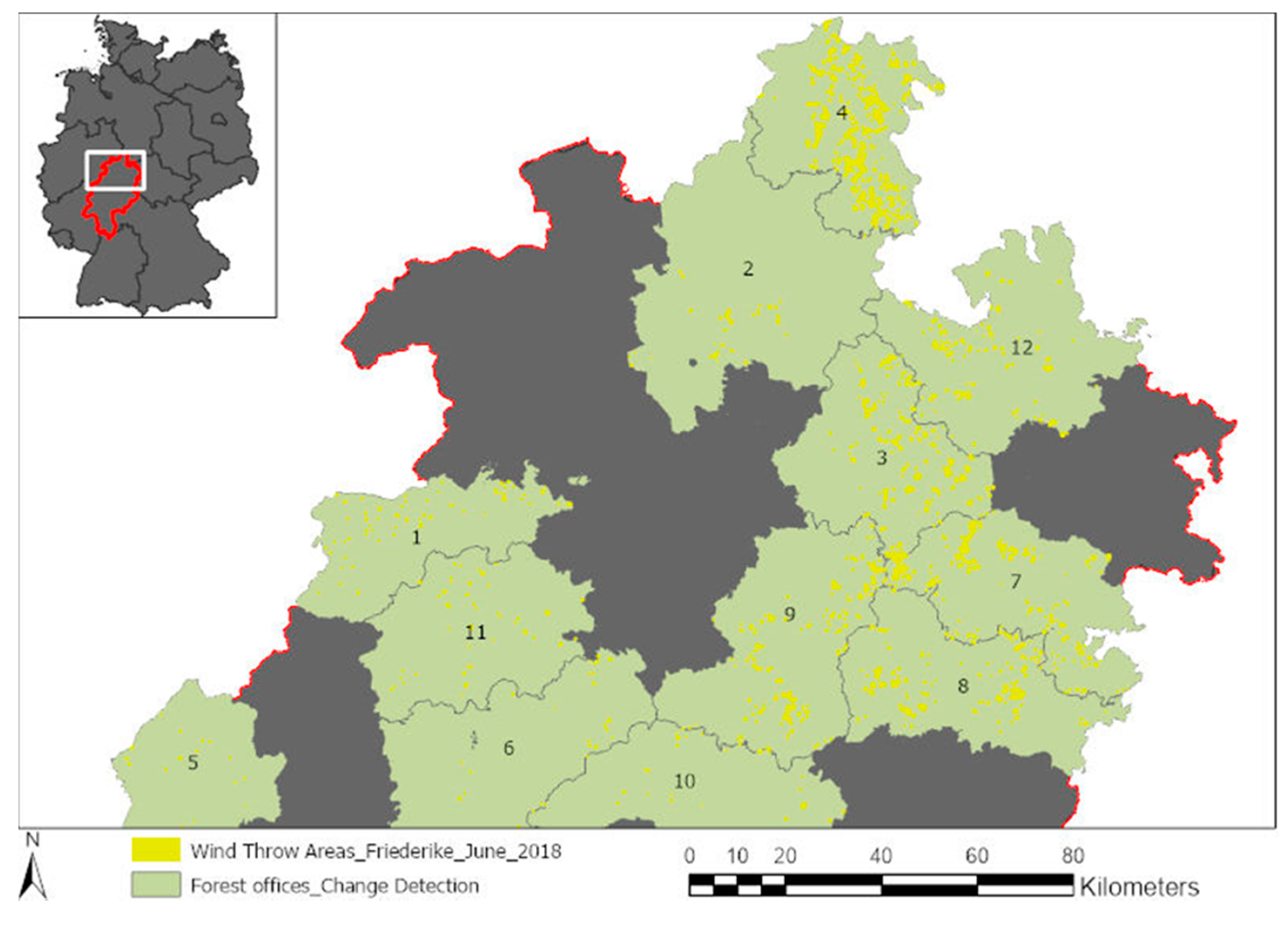
Our study area is the Hessian state forest in the federal state of Hesse, Germany (Figure 1). The total area of Hesse is 21,115 km2 [31] of which 39.8% [32]/42.3% [33] is forest area, that can be divided into 38.2% state forest (state), 36.3% corporate forest, 24.5% private forest and 1.1% state forest (federal) [33].
The region is dominated by deciduous trees (Table 1) with 58% hardwoods in the state forest. Coniferous trees only constitute 42% of the area. Beech trees (Fagus sylvatica L.) have the highest percentage of the tree species composition with about 35%. The second most important tree species of the deciduous wood is oak (Quercus sp. L.) with 10%. Other broadleaf tree species include maples (Acer sp. L.), ashes (Fraxinus excelsior L.), lime trees (Tilia sp. L.), birches (Betula sp. L.), alders (Alnus glutinosa L.), hornbeams (Carpinus betulus L.), willows (Salix sp. L.), poplar (Populus sp. L.), walnut trees (Juglans sp. L.) and species of the Prunus (L.) genus. They account for approx. 13%.
Among the coniferous trees, spruce (Picea abies L., 21%) is the most abundant tree species, followed by pine (Pinus sylvestris L., 11%).The rest consists of other coniferous species such as Douglas fir (Pseudotsuga menziesii Mirb.), larch (Larix sp. Mill.) or fir (Abies alba Mill.).

2.2. Digital Orthophotos

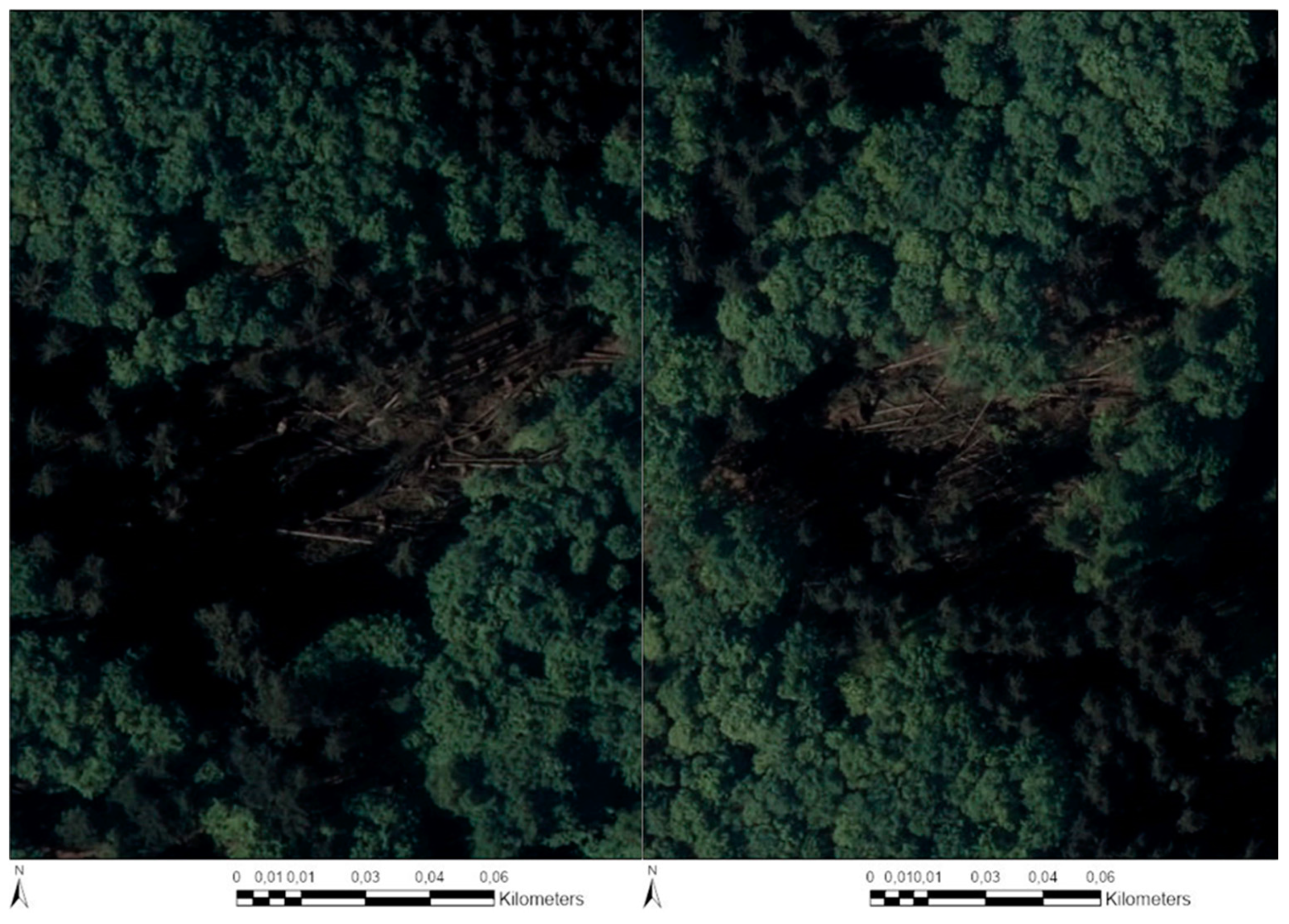
Digital ortho photographs (DOPs) from June/July 2018 (after the storm Friederike) with a spatial resolution of 20 cm were created by the State Surveying Office of Hesse (= HVBG = Hessische Verwaltung für Bodenmanagement und Geoinformation). They consist of 4 bands: red, green, blue and an intensity band (RGBI). Each image had a tile size of 10,000 × 10,000 pixels. The data was used for intensive pre-processing of the labels (see Section 3) and for a qualitative assessment of the final results.

2.3. Labels

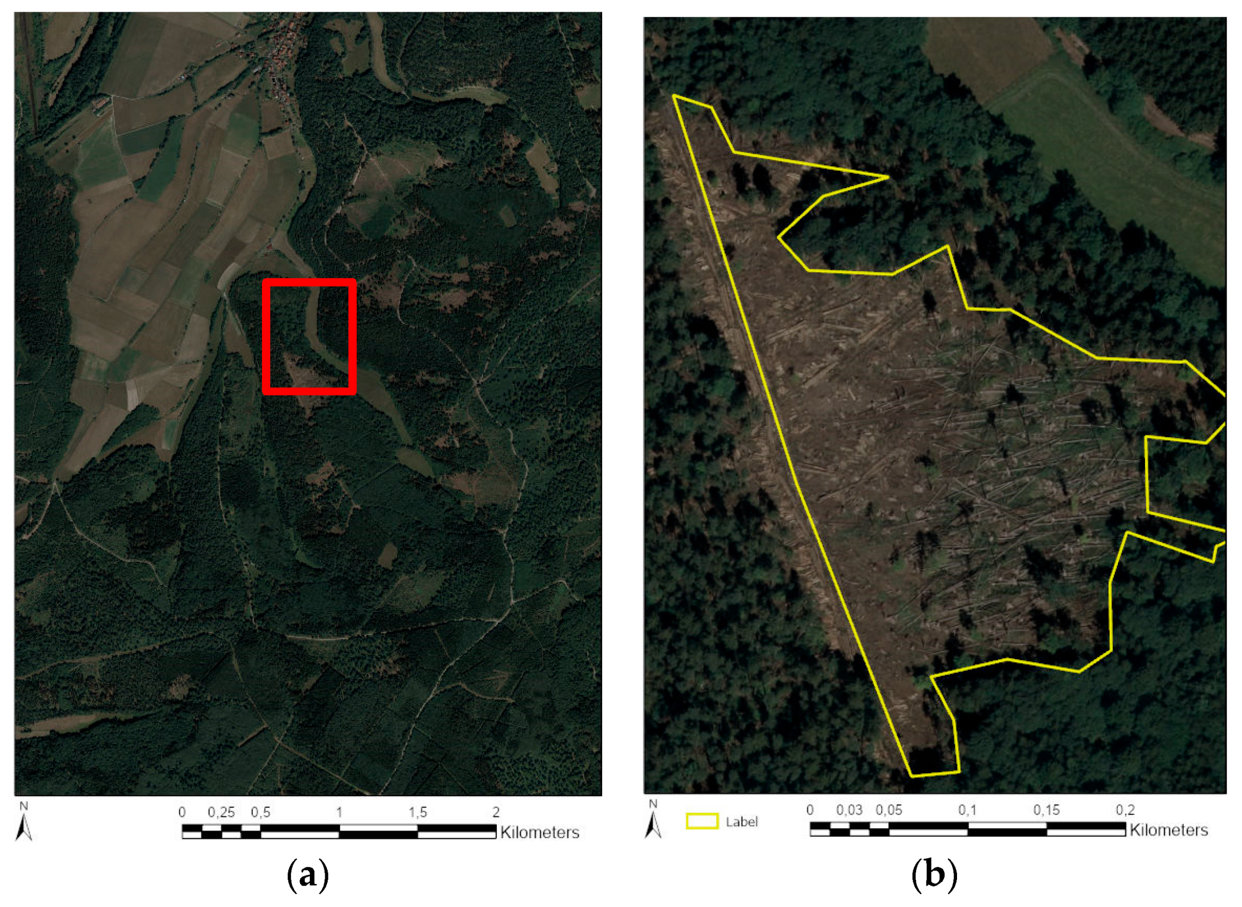
Labels were obtained from a change detection carried out by the GIS Analysis department at HessenForst based on the orthophotos (Figure 2)
The data only covers a limited area in the northern part of the federal State of Hesse (see Figure 1), which does not include all HessenForst operations, but only Frankenberg (1), Wolfhagen (2) Melsungen (3), Reinhardhagen (4), Herbron (5), Kirchhain (6), Rotenburg (7), Bad Hersfeld (8), Neukirchen (9), Romrod (10), Burgwald (11) and Hess. Lichtenau (12). One reason is that the storm caused most damage there, another is that no other data was available at that time. Labels do not include any private, communal forest areas or forest areas managed by the Federal Forestry Office.
In total, there were 1599 labels of varying size. These ranged from very small patches of 0.1054 ha to extensive damaged areas of 34.5428 ha. Areas smaller than 0.1 ha were not included in the analysis by the GIS Analysis department.

2.4. Sentinel-2 Data

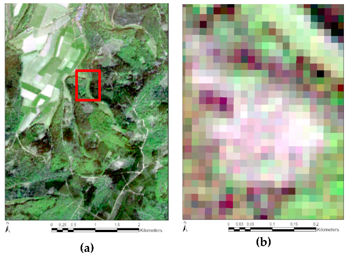
Thirty-two Level-2A Sentinel-2 scenes were acquired via the Copernicus Open Access Hub. Each image has an extent of 100 × 100 km, at a spatial resolution of 10 m, 20 m, and 60 m. The granules are provided in the UTM/WGS84 projection. All images are from a time period after the storm with April 2018 being the latest date and were selected in a way to obtain areal coverage with a minimum of cloud cover (Table 2). Figure 3 shows an example for a cloud-free Sentinel-2 image containing damaged areas.
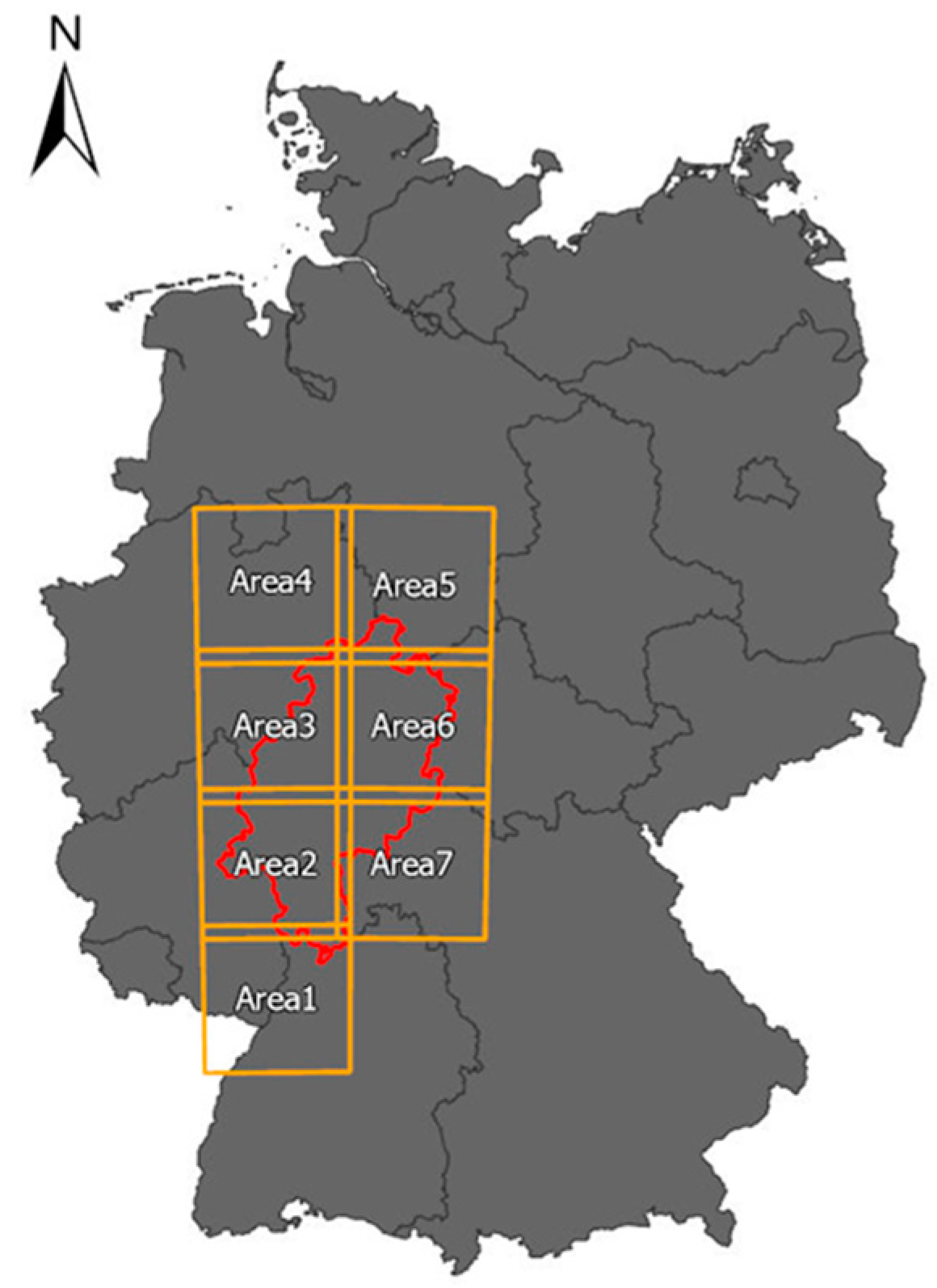
In order to cover the entire area of Hesse, seven sections of the Sentinel data were required (see Figure 4). The data was divided into seven areas for model training, validation and testing (see Section 3).

3. Methods

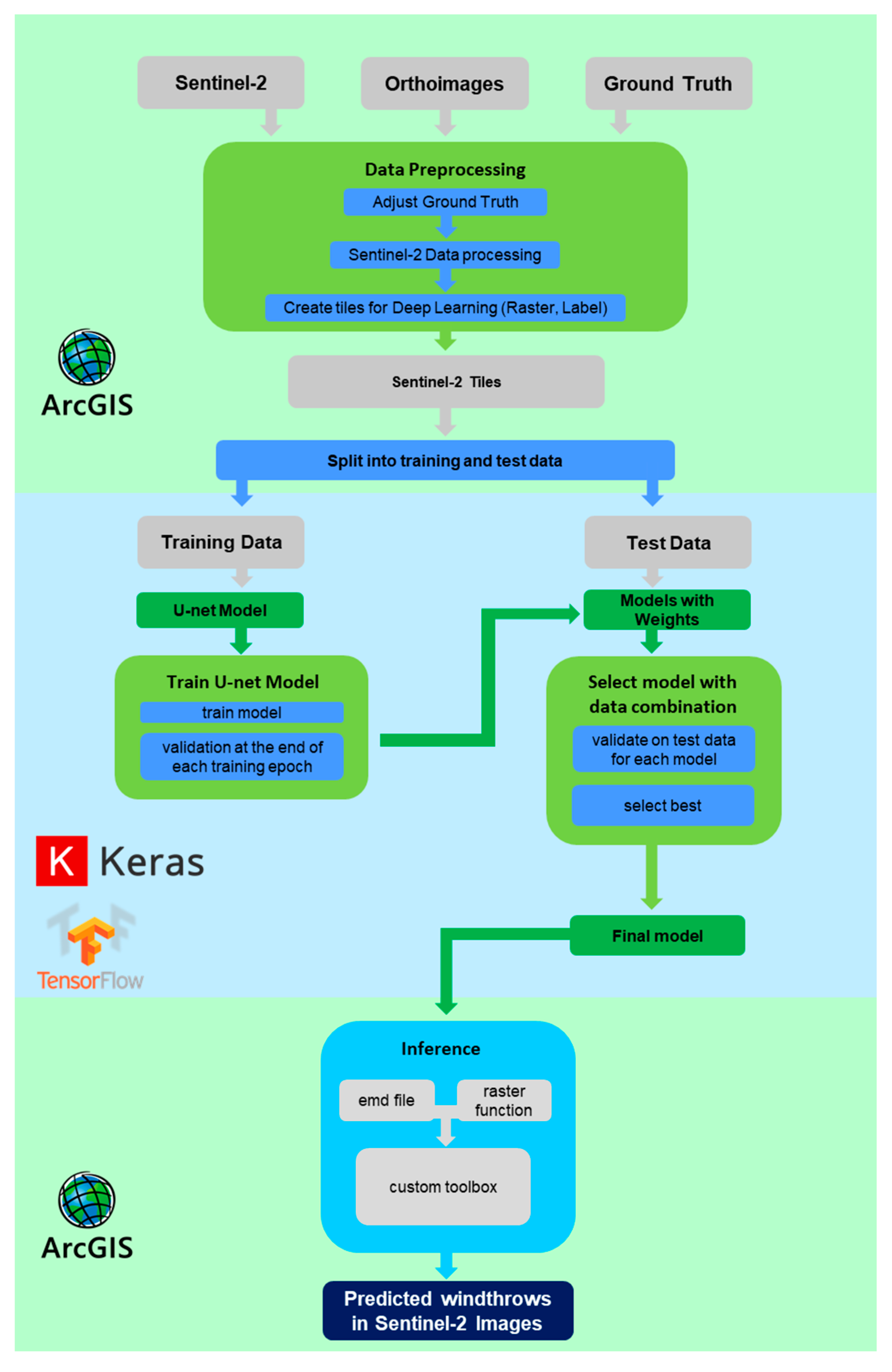
The complete workflow is shown in Figure 5 and will be described in the following sections.

3.1. Preprocessing

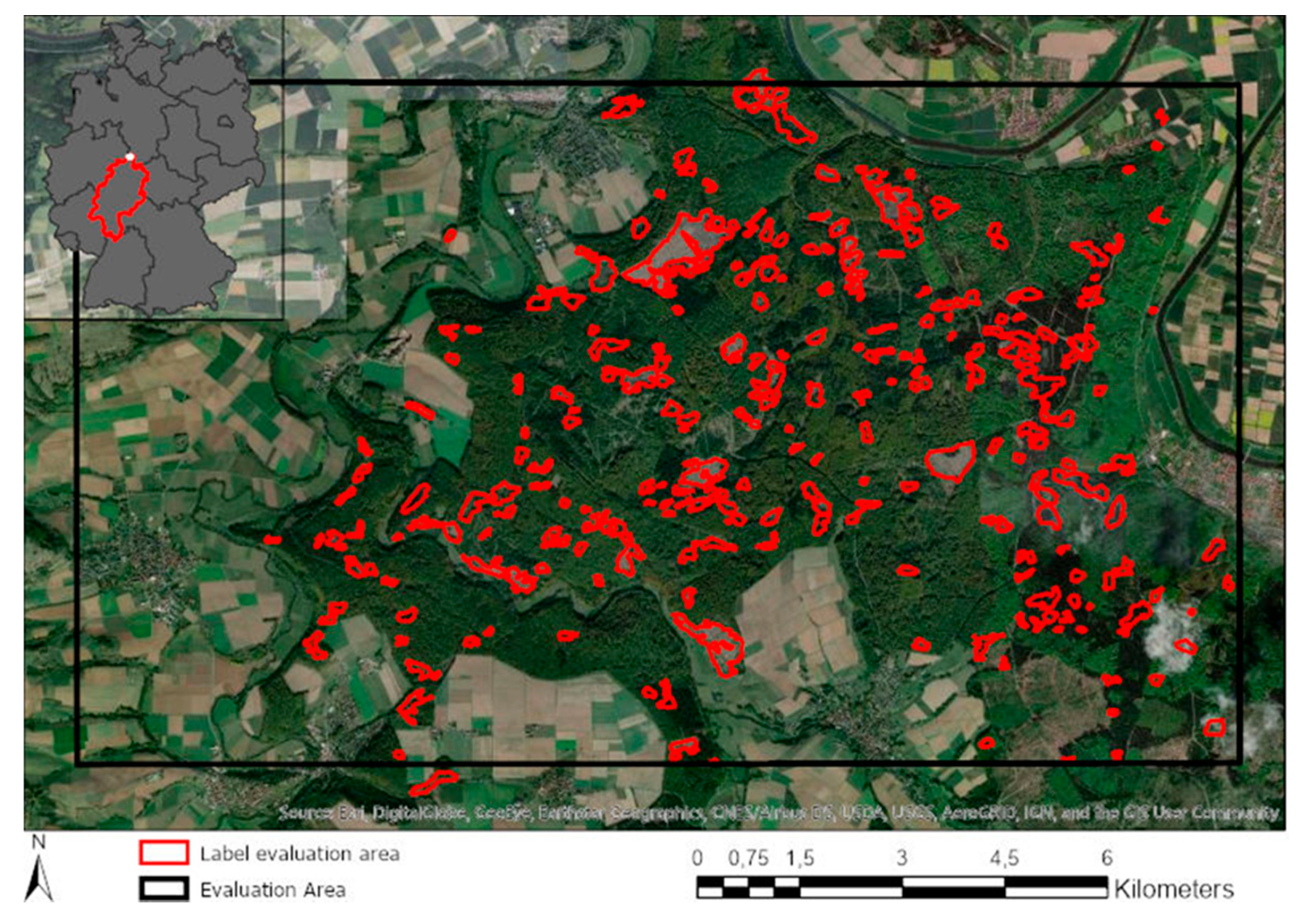
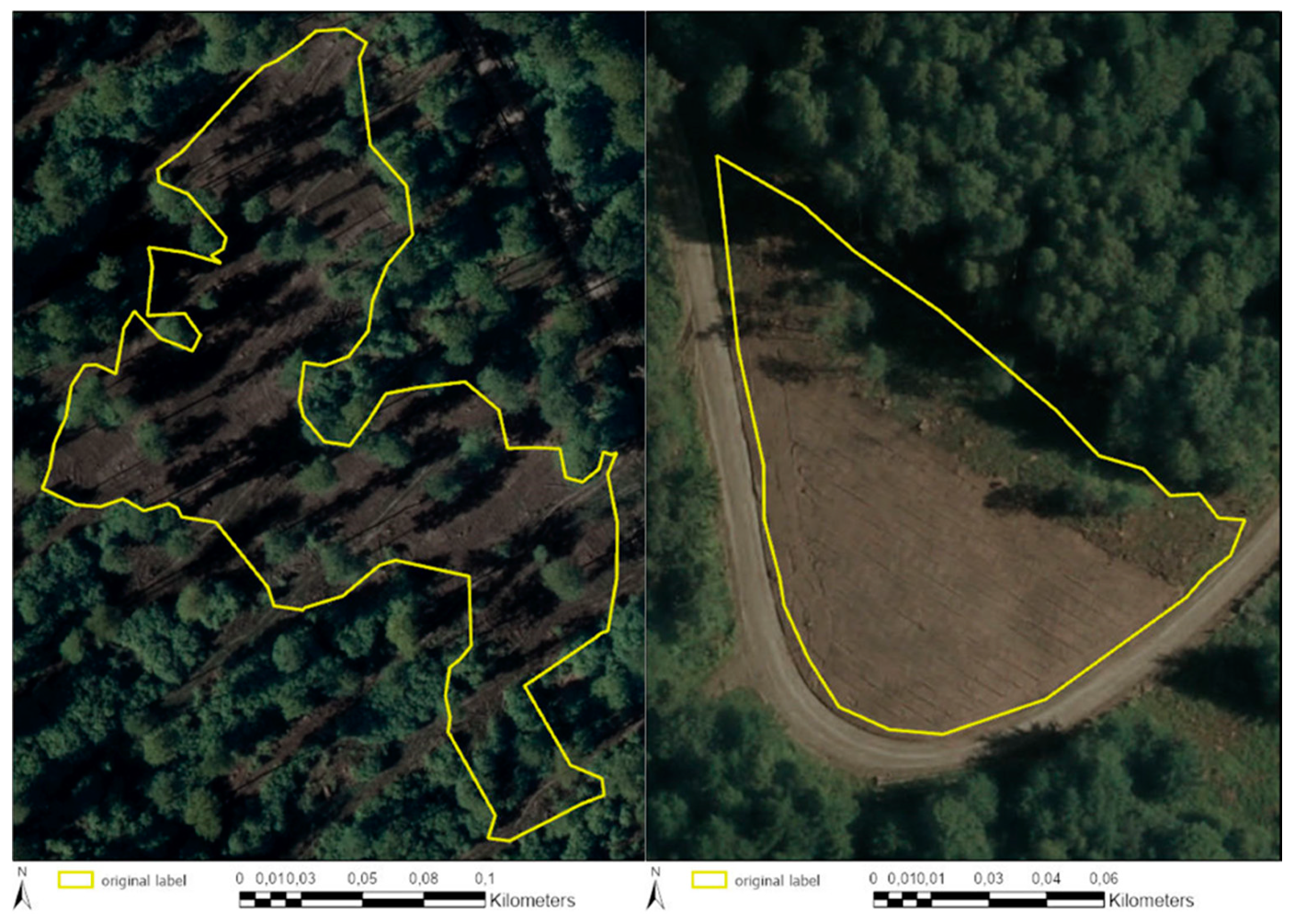
As the provided labels—also called ground truth in the field of remote sensing—were not consistent, we used the DOPs for a profound revision. In particular, shadowy forest edges were corrected extensively. Furthermore, for part of Area5, besides the revision, a complete digitization of previously not digitized damaged areas was carried out to create a reference area for final accuracy assessment. This was necessary as the original labels do not contain private forests and were sometimes not complete (see Figure 6).
Area3, Area5 and Area6 contain most of the labels provided and the respective 12 Sentinel-2 images (Table 2) were selected for modelling. The Level-2A data is already corrected for atmospheric disturbance but had to be cropped to remove artefacts and some clouds. Furthermore, only the 10 m and 20 m bands were used and had to be stacked and resampled to a common spatial resolution of 10 m.
The corrected data (Sentinle-2 and corresponding labels) were then exported as RCNN masks using the Export Training Data for Deep Learning Toolbox in ArcGIS Pro as input for the model. We selected three different tile sizes for our experiments (Table 3). Depending on the tile size, the ratio between damage and no damage changes and leads to different values of class imbalance (Table 3).
The exported dataset was split into training data (Area3 and 6) and testing data (Area5). Area5 contains ca. 17% of the labels and is representative for the study area and therefore well-suited for obtaining representative test metrics.
The tiles were uploaded to a virtual machine (VM) at the Leibniz Supercomputing Centre (LRZ). The utilized single node system, running under Ubuntu 18.04 LTS, consisted of a CPU with 16 cores, 240 GB of RAM, a NVIDIA Tesla P100 PCIe with 16 GB and an 800 GB PCIe SSD.
At the VM Image Normalization was used to reduce the value differences of the 16-bit integer image labels. The individual pixel values were normalized to a value between 0 and 1 as 32-bit floating-point numbers for all channels. Additionally, geometric data augmentation was used to increase the amount of data and to enhance the robustness of the model. Three basic augmentation methods were used: 90° rotation, horizontal flip and vertical flip leading to an eightfold increase of the data.

3.2. Model Implementation

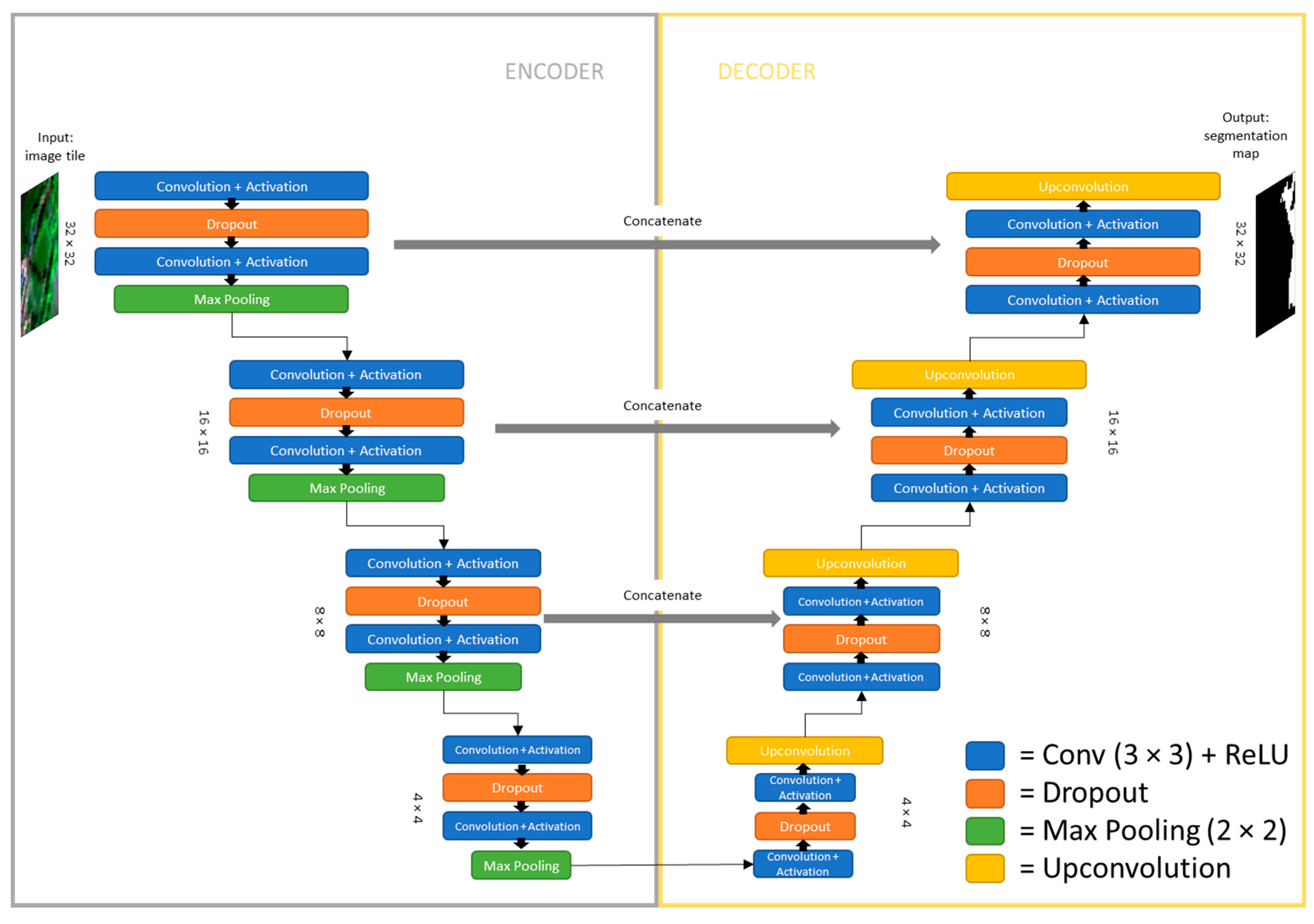
For the model implementation, a modified U-Net [34] architecture was used as it only requires a relatively small data set compared to other architectures like VGG19 or DeepLab. It was originally developed for medical image segmentation and is getting quite popular in the field of remote sensing. The architecture learns in an end-to-end setting and includes an encoder (feature extractor). In the encoding path, a large number of feature maps with reduced dimensionality are produced while the decoding path is used to produce segmentation maps (same size as input) by up-convolutions. Figure 7 shows our final implementation of the architecture. To compensate the class imbalance in our data, we used a Weighted Binary Cross Entropy loss function (see Equation (1)), which increases the impact of the error of one class compared to others by adding weights (w1, w2) to the equation. As an optimizer, we used a modification of stochastic gradient descent, the Adam optimizer (see Equation (2)) [35].
L = 1 N i = 1 N [ y i log ( y ^ i ) w 1 + ( 1 y i ) log ( 1 y ^ i ) w 2 ]
w ( t + 1 ) = w ( t ) μ m ^ w ν ^ w + ϵ m ^ w = m w t + 1 1 β 1 t + 1           ν ^ w = v w t + 1 1 β 2 t + 1 m w t + 1 = β 1 m w t + ( 1 β 1 ) w L ( t ) v w t + 1 = β 2 v w t + ( 1 β 2 ) ( w L ( t ) ) 2

3.3. Evaluation Metrics

One of the most common metrics for measuring the performance of neural networks is the accuracy (Equation (3)). However, due to high class imbalance between the damaged and non-damaged pixel (see Table 3) the metric on its own is not adequate. Therefore, we also report the Intersection over Union (IoU) (Equation (4)), which shows how many pixels are correctly classified as damage compared to the sum of actual and classified damaged pixels and is better suited to assess the model performance in our setting. The prediction of the Network is an image scaled between 0 and 1 (pseudo-probability) and is converted to a binary classification by setting a threshold. For validation, the threshold was chosen at the maximum value for the IoU.
A c c u r a c y =   T P + T N T P + T N + F P + F N
I o U =   T P T P + F P + F N
TP = true positive; TN = true negative; FP = false positive; FN = false negative.

3.4. Postprocessing Geoprocessing Tool

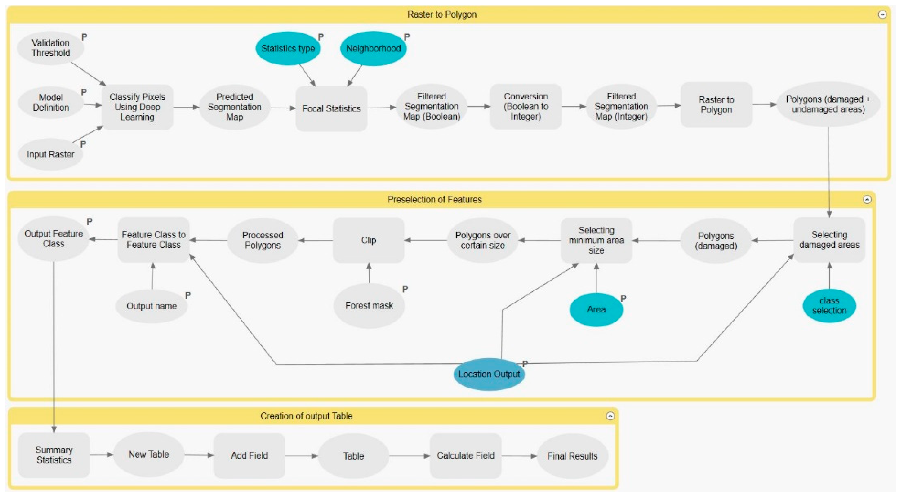
Trained models can be loaded into the tool “Classify Pixels Using Deep Learning” using an emd file that holds some metadata with respect to the model as well as a custom Python function. As some post-processing helps to improve the final product, model builder was used to create a post-processing chain (Figure 8). This includes statistical smoothing, elimination of very small areas and the conversion to polygons with calculated affected areas. The statistics to be used as well as the size of the minimum area are parameters that can be chosen by the analyst.

3.5. Experiments

We used an iterative approach for developing the best model structure as well as the appropriate input data. As we can only compare different settings when only changing one parameter while keeping all other parameters fixed, this required several experiments: For hyperparameters we tested the input tile size, the learning rate as well as the model depth. Additionally we performed tests with respect to the input data itself as the model can either be trained on all data or after applying a mask to only train on the state forest areas as well as on all 10 bands or just the ones containing most information.
The initial parameters were selected based on the model of Deigele et al. [30], who achieved best results in a similar setting (learning rate 0.001, batch size 20, model depth (8,16,32,64,128)). In the following we will briefly describe each experiment:
  • Tile size: Using the above specified settings we tested for tile sizes of 32 × 32, 64 × 64, 128 × 128 and 256 × 256.
  • Learning rate: Using the same settings as in experiment one and a tile size of 32 × 32 different learning rates were tested: 0.1 to 0.0001. A very small learning rate means that the model needs to very long to train, but a big learning rate might cause the model to not converge.
  • Reducing the tiles to areas within the state forest of Hesse: Using the provided mask we tested to train the model, on this area only, as we can exclude private forests that are not labelled, as well as other landcover types. This also means that the number of tiles is reduced and depends on the tile size that was changed during the experiment (the bigger the tile size, the less data).
  • Input spectral bands: To estimate the redundant data in the Sentinel-2 images a Principal Component Transformation (PCA) was conducted. We found that most information was contained in the first two PCs, indicating that using all bands for modelling might not be necessary. Thus, we used only the 10 m spectral bands as those were shown by other studies e.g., Wessel et al. [36] to be the most important ones for forest applications such as tree classification and are, due to the higher spatial resolution, also more appropriate for feature extraction. This experiment was conducted with tile sizes of 32 and 64.
  • Testing and Transfer study: The model with the highest accuracy in the previous experiments was then tested on an unseen area, a part of Area5 (see Section 3.1).

4. Results

4.1. Results from Experiments

Results for all experiments described in the previous section are presented in the same order and were evaluated using the IoU accuracy metric as well as the computation time.
Experiment 1 dealt with evaluating the effect of variable tile sizes and the results are summarized in Table 4 for 15 and 30 epochs of training. A tile size of 32 × 32 gave best results but required most computational time. A smaller tile size results in more training samples which might improve the model.
Results from experiment 2 investigating the learning rate are shown in Table 5. We see the best performance at a rate of 0.001 which is in accordance with other studies in deep learning. At a very high learning rate, the model fails to learn while smaller learning rates might require more epochs than the 15 chosen for the experiment to get better.
Results of the last experiment with respect to the model parameters are shown in Table 6. We tested different depths as well as numbers of convolutions per block. The best results were achieved in a setting of (64,32,16,8) while the model with most parameters, (512,256,512,256,512), shows a significant decrease in the IoU as the model runs into severe overfitting on the training data.
Having found the most suitable hyperparameters, experiment 3 aimed at investigating different data inputs and results are summarized in Table 7. The best results were achieved using a small tile size of 32 × 32 as was to be expected due to the reduction of the area to only the state forest, and thus the decrease in training samples (35,297 vs. 16,852). We also see that the IoU is not as good as the model trained on all the data (previous experiments).
With respect to dimension reduction (experiment 4) using only the four 10 m bands, we found results to be slightly inferior to a setting using all bands (Table 8). This indicates that the information contained in the 20 m bands is contributing to the model and therefore all bands will be used in the final model.
Finally, the model with the best values of all previous experiments (tile size 32 × 32, learning rate 0.001, model depth (64,32,16,8)) was trained and tested on all of the data and used for the transfer study in Area5 (experiment 5). The model was trained for 50 epochs to see when overfitting occurs (Table 9, Figure 9). After four epochs the model was trained best, after that, the validation loss decreased and indicated slight overfitting. The final accuracy for testing is 93% while the IoU is 0.45. For the evaluation area, the accuracy is almost the same while the IoU is slightly better with 0.47. This indicates that the model detects damage that is not labelled as the labels were significantly improved for a part of Area5 (compare section study area).

4.2. Inference Using the New Geoprocessing Tool and Qualitative Assessment of the Results

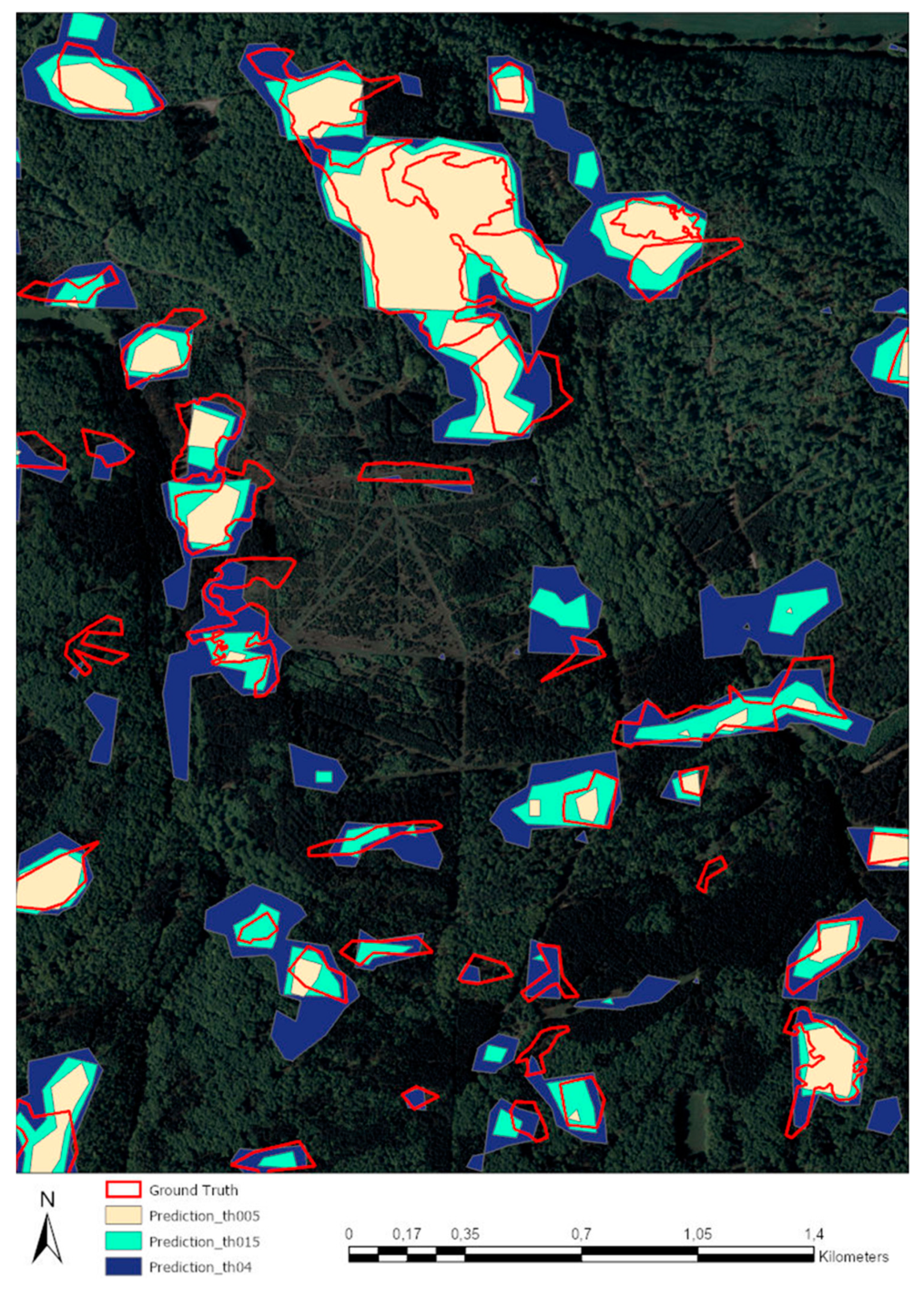
The inference for the best model was calculated in ArcGIS Pro for Area5 using our custom toolbox using circular statistics (median, Units type = Cell, Radius = 1), a batch size of 1 and 0 padding. As the tool allows the user to set the threshold that converts the prediction into a binary classification, we tested three different thresholds to compare the resulting predictions (not only the threshold that maximizes the IoU parameter). The thresholds used were 0.15 (best IoU), 0.4 and 0.05. Figure 10 shows a representative subset of this area with all three predictions overlain on the high-resolution orthophotos. The visual comparison shows the trade-off between finding all damaged areas but having healthy forest included in the damaged class vs. not detecting all damage but having less false positives. The threshold of 0.15 achieves best overall results and is closest to the damaged area calculated from the labels (312.10 ha vs. 133.02 ha at a threshold of 0.05, 266.15 ha at a threshold of 0.15 and 540.74 ha at a threshold of 0.4).
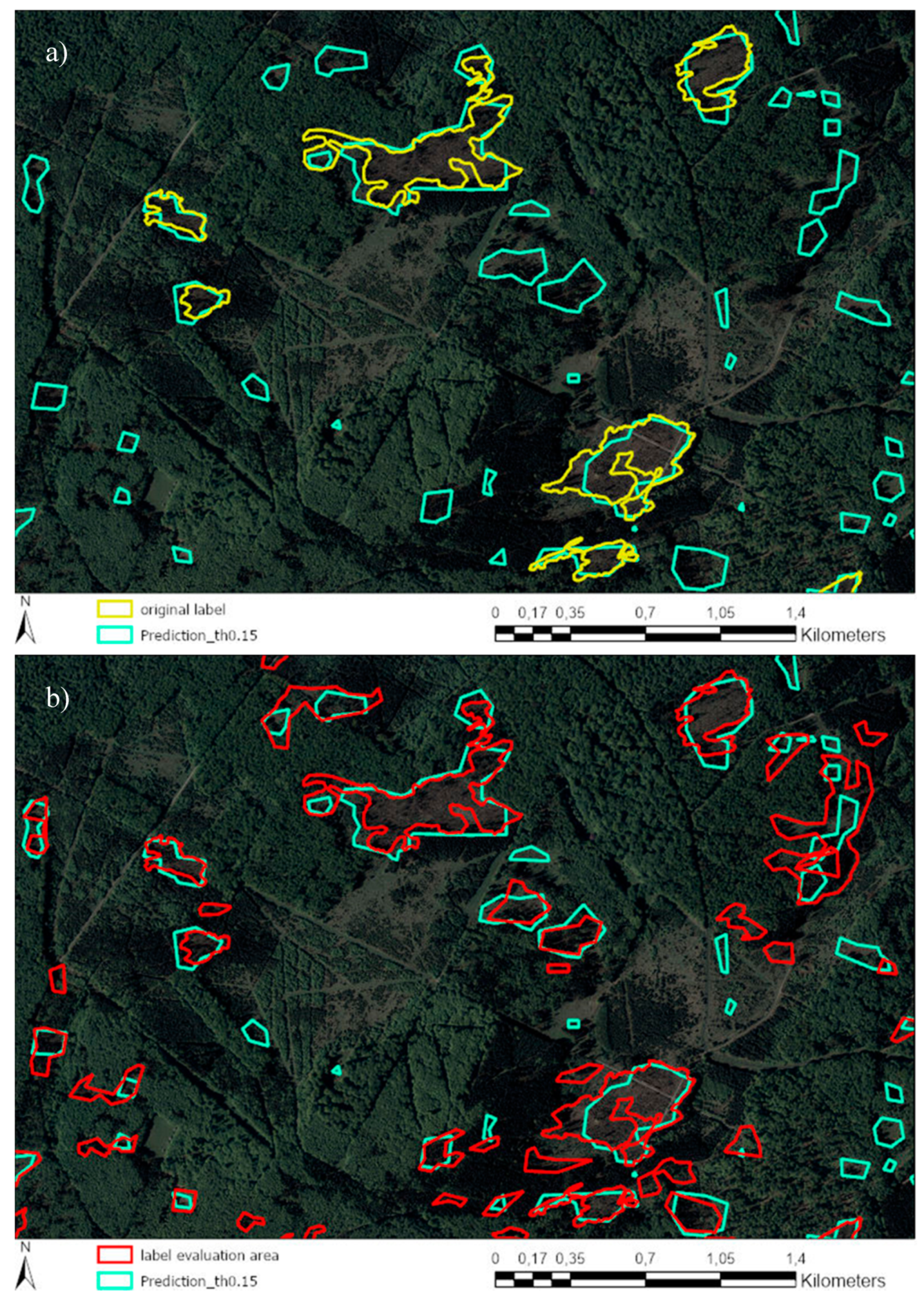
As described in the data section, all labels for the evaluation in Area5 were extensively revised. To assess the impact of the inaccurate and incomplete labels, we compared the old vs. the revised labels and the predictions resulting from the model (Figure 11). This gives some insights about how the model behaves and is capable to generalize while learning on faulty labels.
While all previously labelled damage was identified by the model, additional areas were also detected as damage. Compared to the revised set of labels, we find that part of the additional predictions is actual damage and only few predictions are wrong. This indicates that the model trains reasonably well even on inaccurate and incomplete labels.
Looking more closely at some of the predicted areas that do not match labels, we find that some of the false positives are actually windthrows that were overlooked in the revision (Figure 12a,b) while others are wrong predictions (Figure 12c,d) in areas of harvesting activities or no recognizable damage at all. After a detailed examination of all areas in the evaluation area that did not have any labels, we estimate that ca. 43% were correctly identified as storm damage. Most of the other areas were timber harvesting measures.

5. Discussion

Results highlight the potential of Sentinel-2 data and Deep Learning for rapid damage assessment but also show several problems with respect to the data and other limitations involved. In the following we will discuss the results, and also limitations of the methods and compare them to other approaches.

5.1. Discussion of the Results and Limitations of the Approach

The overall accuracy of 93% and IoU of 0.47 are quite good for a first damage assessment but cannot compete with other results achieved using deep learning in the computer vision community. In the following we will discuss the problems involved in the data, especially the labels from HessenForst.
To begin with, the dataset was a very small one, with the labels consisting of 1599 digitized polygons equivalent to 11,310 tiles when exporting at a size of 32 × 32 (that gave best results). Even after data augmentation the number of tiles (90,480) is small compared to, for example, ca. 14 million samples contained in the ImageNet dataset [37]. This was the reason for choosing U-Net in the first place as it is better suited for smaller datasets. The second limitation is due to a problem that is known as incomplete and inaccurate labelling as defined by Zhou et al. [38] with respect to weakly supervised learning. The first term refers to an incomplete set of labels as was the case in our setting due to the missing labels from the private forests as well as missing labels for overseen damaged areas and areas smaller than 0.1ha that were not digitized at all (compare Figure 13). The latter term refers to the bad quality of the labels (compare Figure 14) that was not perfect even after extensive pre-processing and corrections. This was the reason to create good labels for the evaluation area in the Sentinel section Area5 that was used for testing. Even though deep learning architectures tend to better generalize than traditional algorithms, these problems affect the quality of the predictions significantly and suggest that better labels would be needed to improve results and to make the model more robust.
Another problem is a difference between labels and the size of the damaged area immediately after the storm on the Sentinel data due to, for example, immediate removal of adjacent trees to prevent bark beetle infection. This can potentially lead to further learning on inaccurate data. Figure 15 shows an example for a forested area in the Sentinel image that was already cut down at the time of the DOP collection and thus labelling.
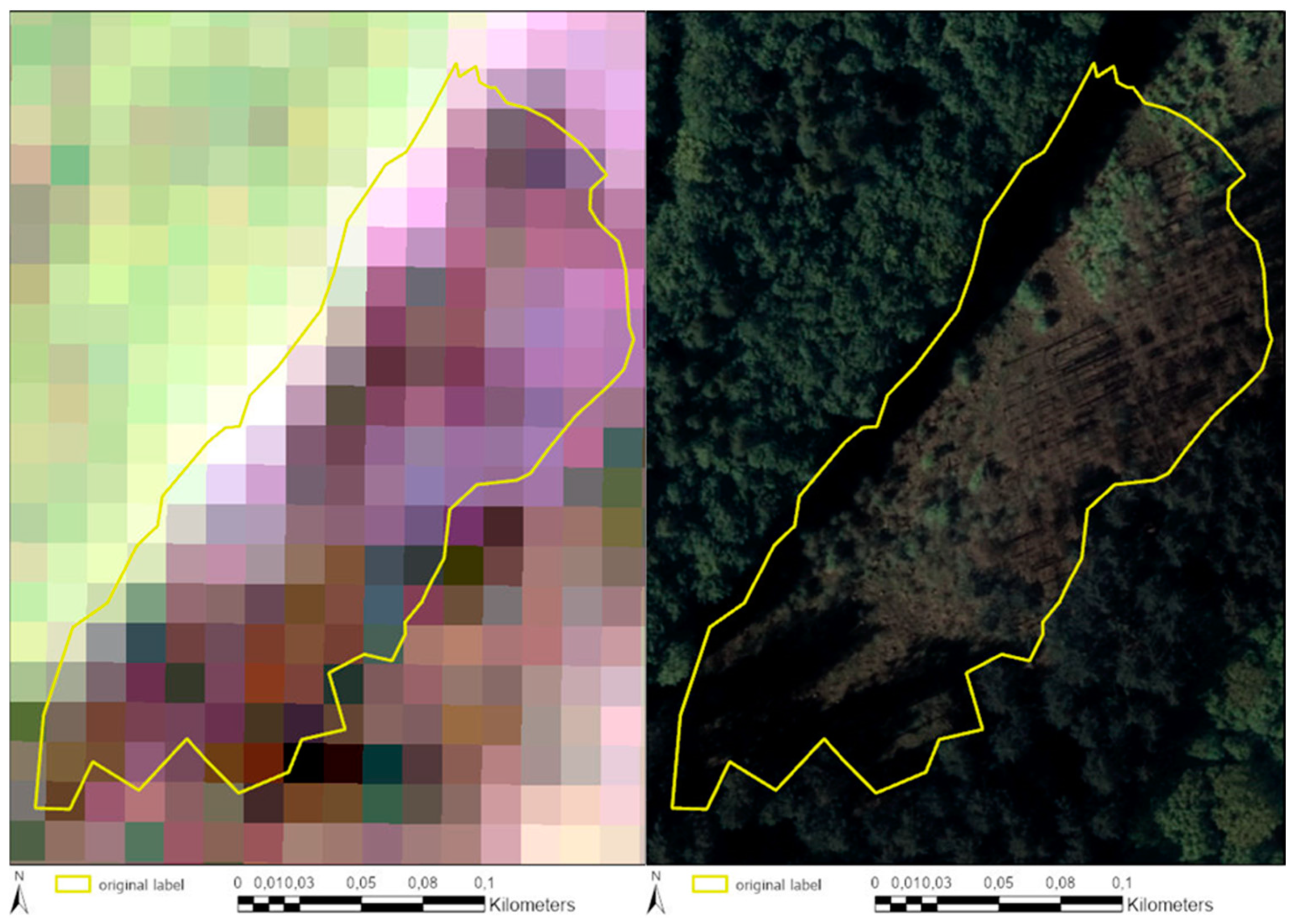
Besides problems arising from inaccurate and incomplete labelling, there are also limitations with respect to the Sentinel-2 input data. While the data is freely available and the acquisition of images is, in an ideal case, every five days, getting appropriate image coverage can take some time due to cloud cover. In our case, this was three months (compare Table 2). Furthermore, the spatial resolution of 10 m or 20 m is a big limitation compared to high-resolution DOPs. Features like fallen trees are not visible at that resolution and mapping can therefore only delineate damaged areas on a much coarser level than using DOPs (compare Figure 16).
With respect to changing the input data, we found that results for only including state forests are worse than for including the whole area (Table 4). A model trained only on the forest will result in a prediction with lots of artefacts in urban and rural areas as the network has never seen these features before. Such an approach is only suitable if a forest mask is available and all artefacts can be removed in a clipping operation. Another approach would be to include more classes in the problem, but this would require a lot of labelling work. Similarly, using a reduced number of bands also resulted in slightly worse predictions even though results from only using the four 10 m bands can almost compare to using all bands. This is in agreement with the findings of Wessel et al. [36] who found the 10 m bands to be most useful for tree species classification.

5.2. Comparison to Other Remote Sensing Methods

A comparison of this work with other studies is difficult because of the limitations discussed above and the different sensors used. Nevertheless, in the following we give a comparison to other approaches and evaluate the respective advantages and disadvantages.
One of the biggest differences of the presented method to other approaches based on change detection is that the latter approaches always require two images, before and after the storm e.g., [15,19,23] while CNNs only require a post-storm image. This is due to the nature of CNNs as efficient feature extractors while change detection relies on finding differences between images from different times of collection. This allows the application of CNNs in areas where no pre-storm data is available which might be an advantage for forest agencies.
In comparison to approaches based on active systems, radar data is not dependent on meteorological influences. However, studies by Eriksson et al. [17] and Ningthoujam et al. [18] indicate that the spatial resolution of SAR images is crucially important. Eriksson et al. [17] postulate that a spatial resolution of less than 10 m is recommended for good damage detection. Ningthoujam et al. [18] also show that a finer spatial resolution leads to better results (6 m = 70%; 20 m = 63%). This is in agreement with our findings using Sentinel-2 data with a maximum spatial resolution of 10 m compared to previous works by Deigele et al. [30] working on DOPs and PlanetScope data (3 m). Nevertheless, our results are slightly better in terms of accuracy than results of Ningthoujam et al. [18], Tanase et al. [14] (92.5% vs. 84%) or Rüetschi et al. [19] (92.5% vs. 85%). However, note that due to class imbalance issues this is not a good metric compared to the IoU. Scattered windthrow caused poorer results on average than areal windthrow in the study of [19], whereas this work showed that even smaller damaged areas could be successfully detected.
A comparison to methods using ALS that allows the detection of lying trunks [3,20,21] due to the high spatial resolution, is more difficult. Honkavaara et al. [13], for example, achieved an accuracy of 100% for larger damaged areas (m2) while the accuracy for smaller areas was reduced to half.
In comparison to studies using passive sensors, the accuracies are strongly dependent on the chosen method and spatial resolution. While Zhu et al. [26] achieved better results with LANDSAT data and a pixel-based method (92.5% vs. 95%), Haidu et al. [25] was only able to achieve an accuracy of 86% for scattered windthrow following a “dark object” approach by Huang et al. [39] in combination with a Disturbance Index and the image classification of before and after the storm. With respect to object-based approaches, the studies of Chehata et al. [23] (92.5% vs. 87.8%) and Duan et al. [22] (92.5% vs. 92.5%) are comparable with the results of this work. However, Duan et al. [22] used high-resolution UAS data for their analysis, making a direct comparison of biased accuracies. With a combination of a pixel-based approach for small areas and an object-based approach for the detection of larger areas, Einzmann et al. [27] achieved an overall accuracy of 90%, which is similar to our results.
The results of Hamdi et al. [29] and Deigele et al. [30], who also used CNNs but on high-resolution DOPs and PlanetScope data are superior to our results (IoU of 0.67 and 0.73 (DOP), 0.55 (Planet) respectively compared to 0.46 in this study), however the data is not freely available and might be expensive.

6. Conclusions and Outlook

We could show that deep learning approaches based on Sentinel-2 data are suitable for detecting major calamities caused by windthrow and subsequent bark beetle damage. As Sentinel-2 data is freely available, this can help forest management in an early stage of disaster management. Results, however, are inferior to results from high spatial resolution data. The study also highlights the importance of accurate and complete labels for training the model. This means that damage documentation in different forest departments needs to be standardized to create comprehensive data for training a model capable of generalizing well.
As the approach is still novel in forestry, we hope that this kind of data will be available in the future to further assess these methods for efficient forest management. The integration of the models into the ArcGIS Platform allows a complete workflow from damage detection and post-processing to the coordination of fieldwork and the use of mobile applications for documentation in the forest. The authors see a great potential in AI-based approaches in remote sensing that is still somewhat hindered by the problems involved in weakly supervised learning.

Author Contributions

Conceptualization, M.B., M.W. and D.S.; Writing original-draft, D.S. and M.B. All authors have read and agreed to the published version of the manuscript.

Funding

This research received no external funding.

Acknowledgments

We would like to thank HessenForst for providing the data for this study. Furthermore, we thank Esri Germany for providing the necessary resources for this study.

Conflicts of Interest

The authors declare no conflict of interest.

References

  1. Gardiner, B.; Blennow, K.; Carnus, J.M.; Fleischer, P.; Ingemarsson, F.; Landmann, G.; Lindner, M.; Marzano, M.; Nicoll, B.; Orazio, C.; et al. Destructive Storms in European Forests: Past and Forthcoming Impacts. 2010. Available online: https://ec.europa.eu/environment/forests/pdf/STORMS%20Final_Report.pdf (accessed on 3 February 2020).
  2. Seidl, R.; Schelhaas, M.-J.; Rammer, W.; Verkerk, P.J. Increasing forest disturbances in Europe and their impact on carbon storage. Nat. Clim. Chang. 2014, 4, 806–810. [Google Scholar] [CrossRef] [PubMed] [Green Version]
  3. Chirici, G.; Bottalico, F.; Giannetti, F.; Del Perugia, B.; Travaglini, D.; Nocentini, S.; Kutchartt, E.; Marchi, E.; Foderi, C.; Fioravanti, M.; et al. Assessing forest windthrow damage using single-date, post-event airborne laser scanning data. For. Int. J. For. Res. 2018, 91, 27–37. [Google Scholar] [CrossRef] [Green Version]
  4. Forzieri, G.; Pecchi, M.; Girardello, M.; Mauri, A.; Klaus, M.; Nikolov, C.; Rüetschi, M.; Gardiner, B.; Tomaštík, J.; Small, D.; et al. A spatially explicit database of wind disturbances in European forests over the period 2000–2018. Earth Syst. Sci. Data 2020, 12, 257–276. [Google Scholar] [CrossRef] [Green Version]
  5. Mölter, T.; Schindler, D.; Albrecht, A.; Kohnle, U. Review on the Projections of Future Storminess over the North Atlantic European Region. Atmosphere 2016, 7, 60. [Google Scholar] [CrossRef] [Green Version]
  6. Fink, A.H.; Brücher, T.; Ermert, V.; Krüger, A.; Pinto, J.G. The European storm Kyrill in January 2007: Synoptic evolution, meteorological impacts and some considerations with respect to climate change. Nat. Hazards Earth Syst. Sci. 2009, 9, 405–423. [Google Scholar] [CrossRef] [Green Version]
  7. Forster, B.; Meier, F. Sturm, Witterung und Borkenkäfer. Risikomanagement im Forstschutz; Merkblatt für die Praxis No. 44. 2010. Available online: https://www.dora.lib4ri.ch/wsl/islandora/object/wsl%3A9138/datastream/PDF/view (accessed on 5 April 2020).
  8. Seidl, R.; Rammer, W. Climate change amplifies the interactions between wind and bark beetle disturbances in forest landscapes. Landsc. Ecol. 2017, 32, 1485–1498. [Google Scholar] [CrossRef] [PubMed] [Green Version]
  9. Hanewinkel, M.; Peyron, J.L. The economic impact of storms. In Living with Storm Damage to Forests What Science Can Tell Us; Gardiner, B., Schuck, A., Schelhaas, M.-J., Orazio, C., Blennow, K., Nicoll, B., Eds.; European Forest Institute: Joensuu, Finland, 2013; pp. 55–63. [Google Scholar]
  10. Fuhrer, J.; Beniston, M.; Fischlin, A.; Frei, C.; Goyette, S.; Jasper, K.; Pfister, C. Climate Risks and Their Impact on Agriculture and Forests in Switzerland. Clim. Chang. 2006, 79, 79–102. [Google Scholar] [CrossRef] [Green Version]
  11. UN. Sustainable Development Goals: Sustainable Development Knowledge Platform. Available online: https://sustainabledevelopment.un.org/?menu=1300 (accessed on 6 April 2020).
  12. Seitz, R.; Straub, C. »FastResponse«—Die Schnelle Antwort Nach Dem Sturm, LWF Aktuell No. 4. 2017. Available online: https://www.lwf.bayern.de/mam/cms04/informationstechnologie/dateien/a115_fast_response_seitz.pdf (accessed on 5 April 2020).
  13. Honkavaara, E.; Litkey, P.; Nurminen, K. Automatic Storm Damage Detection in Forests Using High-Altitude Photogrammetric Imagery. Remote Sens. 2013, 5, 1405–1424. [Google Scholar] [CrossRef] [Green Version]
  14. Tanase, M.A.; Aponte, C.; Mermoz, S.; Bouvet, A.; Le Toan, T.; Heurich, M. Detection of windthrows and insect outbreaks by L-band SAR: A case study in the Bavarian Forest National Park. Remote Sens. Environ. 2018, 209, 700–711. [Google Scholar] [CrossRef]
  15. Fransson, J.E.S.; Walter, F.; Blennow, K.; Gustavsson, A.; Ulander, L.M.H. Detection of storm-damaged forested areas using airborne CARABAS-II VHF SAR image data. IEEE Trans. Geosci. Remote Sens. 2002, 40, 2170–2175. [Google Scholar] [CrossRef]
  16. Fransson, J.E.S.; Pantze, A.; Eriksson, L.E.B.; Soja, M.J.; Santoro, M. Mapping of wind-thrown forests using satellite SAR images. In Proceedings of the 2010 IEEE International Geoscience & Remote Sensing Symposium, Honolulu, HI, USA, 25–30 July 2010; IEEE: Piscataway, NJ, USA, 2010; pp. 1242–1245, ISBN 978-1-4244-9565-8. [Google Scholar]
  17. Eriksson, L.E.B.; Fransson, J.E.S.; Soja, M.J.; Santoro, M. Backscatter signatures of wind-thrown forest in satellite SAR images. In Proceedings of the IEEE International Geoscience and Remote Sensing Symposium, Munich, Germany, 22–27 July 2012; IEEE: Piscataway, NJ, USA, 2012; pp. 6435–6438, ISBN 978-1-4673-1159-5. [Google Scholar]
  18. Ningthoujam, R.; Tansey, K.; Balzter, H.; Morrison, K.; Johnson, S.; Gerard, F.; George, C.; Burbidge, G.; Doody, S.; Veck, N.; et al. Mapping Forest Cover and Forest Cover Change with Airborne S-Band Radar. Remote Sens. 2016, 8, 577. [Google Scholar] [CrossRef] [Green Version]
  19. Rüetschi, M.; Small, D.; Waser, L. Rapid Detection of Windthrows Using Sentinel-1 C-Band SAR Data. Remote Sens. 2019, 11, 115. [Google Scholar] [CrossRef] [Green Version]
  20. Nyström, M.; Holmgren, J.; Fransson, J.E.S.; Olsson, H. Detection of windthrown trees using airborne laser scanning. Int. J. Appl. Earth Obs. Geoinf. 2014, 30, 21–29. [Google Scholar] [CrossRef]
  21. Mokroš, M.; Výbošťok, J.; Merganič, J.; Hollaus, M.; Barton, I.; Koreň, M.; Tomaštík, J.; Čerňava, J. Early Stage Forest Windthrow Estimation Based on Unmanned Aircraft System Imagery. Forests 2017, 8, 306. [Google Scholar] [CrossRef] [Green Version]
  22. Duan, F.; Wan, Y.; Deng, L. A Novel Approach for Coarse-to-Fine Windthrown Tree Extraction Based on Unmanned Aerial Vehicle Images. Remote Sens. 2017, 9, 306. [Google Scholar] [CrossRef]
  23. Chehata, N.; Orny, C.; Boukir, S.; Guyon, D.; Wigneron, J.P. Object-based change detection in wind storm-damaged forest using high-resolution multispectral images. Int. J. Remote Sens. 2014, 35, 4758–4777. [Google Scholar] [CrossRef]
  24. Chehata, N.; Orny, C.; Boukir, S.; Guyon, D. Object-based forest change detection using high resolution satellite images. Int. Arch. Photogramm. Remote Sens. Spat. Inf. Sci. 2011, XXXVIII-3/W22, 49–54. [Google Scholar] [CrossRef] [Green Version]
  25. Haidu, I.; Furtuna, P.R.; Lebaut, S. Detection of old scattered windthrow using low cost resources. The case of Storm Xynthia in the Vosges Mountains, 28 February 2010. Open Geosci. 2019, 11, 492–504. [Google Scholar] [CrossRef]
  26. Zhu, Z.; Woodcock, C.E.; Olofsson, P. Continuous monitoring of forest disturbance using all available Landsat imagery. Remote Sens. Environ. 2012, 122, 75–91. [Google Scholar] [CrossRef]
  27. Einzmann, K.; Immitzer, M.; Böck, S.; Bauer, O.; Schmitt, A.; Atzberger, C. Windthrow Detection in European Forests with Very High-Resolution Optical Data. Forests 2017, 8, 21. [Google Scholar] [CrossRef] [Green Version]
  28. Blaschke, T. Object based image analysis for remote sensing. ISPRS J. Photogramm. Remote Sens. 2010, 65, 2–16. [Google Scholar] [CrossRef] [Green Version]
  29. Hamdi, Z.M.; Brandmeier, M.; Straub, C. Forest Damage Assessment Using Deep Learning on High Resolution Remote Sensing Data. Remote Sens. 2019, 11, 1976. [Google Scholar] [CrossRef] [Green Version]
  30. Deigele, W.; Brandmeier, M.; Straub, C. A Hierarchical Deep-Learning Approach for Rapid Windthrow Detection on PlanetScope and High-Resolution Aerial Image Data. Remote Sens. 2020, 12, 2121. [Google Scholar] [CrossRef]
  31. Statistisches Bundesamt. Bodenfläche nach Nutzungsarten und Bundesländern. Available online: https://www.destatis.de/DE/Themen/Branchen-Unternehmen/Landwirtschaft-Forstwirtschaft-Fischerei/Flaechennutzung/Tabellen/bodenflaeche-laender.html (accessed on 19 February 2020).
  32. Statistisches Bundesamt. 30% der Fläche in Deutschland Sind Wald, Pressemitteilung Nr. 12; Statistisches Bundesamt: Wiesbaden, Germany, 2019.
  33. Thünen-Institut. Waldfläche [ha] nach Land und Eigentumsart Filter: Jahr=2012. 2012. Available online: https://bwi.info (accessed on 19 February 2020).
  34. Ronneberger, O.; Fischer, P.; Brox, T. U-Net: Convolutional Networks for Biomedical Image Segmentation. 2015. Available online: http://arxiv.org/pdf/1505.04597v1 (accessed on 27 January 2020).
  35. Kingma, D.P.; Ba, J. Adam: A Method for Stochastic Optimization. 2014. Available online: http://arxiv.org/pdf/1412.6980v9 (accessed on 27 January 2020).
  36. Wessel, M.; Brandmeier, M.; Tiede, D. Evaluation of Different Machine Learning Algorithms for Scalable Classification of Tree Types and Tree Species Based on Sentinel-2 Data. Remote Sens. 2018, 10, 1419. [Google Scholar] [CrossRef] [Green Version]
  37. ImageNet. Available online: http://www.image-net.org/ (accessed on 24 March 2020).
  38. Zhou, Z.-H. A brief introduction to weakly supervised learning. Natl. Sci. Rev. 2018, 5, 44–53. [Google Scholar] [CrossRef] [Green Version]
  39. Huang, C.; Song, K.; Kim, S.; Townshend, J.R.G.; Davis, P.; Masek, J.G.; Goward, S.N. Use of a dark object concept and support vector machines to automate forest cover change analysis. Remote Sens. Environ. 2008, 112, 970–985. [Google Scholar] [CrossRef]
Figure 1. Study area. Green areas show the regions included in the change detection: Frankenberg (1), Wolfhagen (2), Melsungen (3), Reinhardhagen (4), Herbron (5), Kirchhain (6), Rotenburg (7), Bad Hersfeld (8), Neukirchen (9), Romrod (10), Burgwald (11) and Hess. Lichtenau (12), while yellow areas show the labels of the storm that caused damage in these regions. Grey areas were not included in the provided labels.
Forests 11 01239 g001
Figure 2. Digital orthophotos used in the project: (a) Example for an image with windthrows. (b) Close up view of the image shown on the left with a partially processed windthrow and corresponding label from the change detection (red square).
Forests 11 01239 g002
Figure 3. Sentinel-2 data used in the project: (a) Example for a Sentinel-2 section with damage. (b) Close-up view of a windthrow in the Sentinel-2 images with a spatial resolution of 10 m (red square in a).
Forests 11 01239 g003
Figure 4. Outlines of the seven sentinel sections with the names assigned to each section.
Forests 11 01239 g004
Figure 5. Workflow of the complete process, divided into three steps for preprocessing, training and postprocessing.
Forests 11 01239 g005
Figure 6. Completely revised evaluation area in the Area5 section of the Sentinel data in northern Hesse with all previously not included damaged areas.
Forests 11 01239 g006
Figure 7. Design of our custom U-Net architecture for 32 × 32 pixels.
Forests 11 01239 g007
Figure 8. Model of the created toolbox in ArcGIS Pro.
Forests 11 01239 g008
Figure 9. Visualization of the training process in TensorBoard over 50 epochs for the loss (orange line = train loss; blue line = val loss) and the mean IoU (orange line = train mean IoU; blue line = val mean IoU) with indicated early stopping point (red line).
Forests 11 01239 g009
Figure 10. Predictions of the final model using different thresholds on a subset of the evaluation area (Digital ortho photographs (DOP) in the background).
Forests 11 01239 g010
Figure 11. Comparison of the prediction with the original and revised labels with a DOP in the background (a) Prediction (turquoise) compared to the original label (yellow). (b) Prediction (turquoise) in comparison to the revised labels (red) of the evaluation area.
Forests 11 01239 g011
Figure 12. Examples of false positives that are true positives (a,b) and false positives that are either due to harvesting (c) or undisturbed forest (d).
Forests 11 01239 g012
Figure 13. Example of small damaged areas as shown in the DOP surrounded by healthy stands that were initially not labeled by HessenForst.
Forests 11 01239 g013
Figure 14. Example for inaccurate labels. Areas that were not damaged by the storm but rather other activities, such as timber harvesting (left) or earthworks (right).
Forests 11 01239 g014
Figure 15. Area labelled as damaged, which still has a tree stand on the sentinel sections but has already been partially cleared on the DOP.
Forests 11 01239 g015
Figure 16. Comparison of the original label (left) with the predicted area (right) based on the spatial resolution of the Sentinel-2 data.
Forests 11 01239 g016
Table 1. Tree species composition of the state forest area in Hesse (HessenForst 2018).
Deciduous Trees∑ =58%Coniferous Trees∑ =42%
tree speciesoakbeecho. deciduous treessprucepineo. coniferous trees
composition10%35%13%21%11%10%
Table 2. Available data in the time period chosen for this study. (× = data available).
Area1Area2Area3Area4Area5Area6Area7
24 April 2018×
20 April 2018×××××××
18 April 2018 ××
12 April 2018 ×
10 April 2018 ××××
8 April 2018 ××
7 April 2018×× ×××
2 April 2018×
21 March 2018 ××
11 March 2018 ×
1 March 2018 × ×
24 February 2018 × ×
14 February 2018××
Table 3. Display of the damaged pixels in the exported tiles based on the size.
Exported Tile SizeUndamaged Pixel in %Damaged Pixel in %
32 × 3292.017.99
64 × 6496.463.54
128 × 12898.071.93
256 × 25699.240.76
Table 4. Results from experiment 1: Effect of different tile sizes. Green background color indicates the best result, while red background highlights the worst result.
15 Epochs30 Epochs
Tile SizeMax IoUMax IoUØ Seconds/Epoch
32 × 320.3960.382625
64 × 640.3380.332424
128 × 1280.2850.284388
256 × 2560.3020.248559
Table 5. Results from experiment 2: Effect of different learning rate. Green background color indicates the best result, while red background highlights the worst result.
Learning RateMax IoUØ Seconds/Epoch
0.1 *0.096582
0.01 **0.107567
0.0010.401550
0.00010.351555
0.000010.317590
* loss and mean Intersection over Union (IoU) are not changing during training. ** loss stagnates but means that IoU is decreasing while training.
Table 6. Results from experiment 2: Different model depth and convolution blocks. Green background color indicates the best result, while red background highlights the worst result.
Model DepthMax IoUØ Seconds/Epoch
8,16,32,64,1280.401550
128,64,32,16,80.368621
8,16,32,64,128,2560.370728
256,128,64,32,16,80.360706
8,16,32,640.398462
64,32,16,80.435471
32,16,80.419434
64,32,160.424447
16,8,16,8,160.409647
512,256,512,256,5120.3171233
Table 7. Results from experiment 3: Using only tiles from the state forest. Green background color indicates the best result, while red background highlights the worst result.
15 Epochs30 Epochs
Tile SizeMax IoUMax IoUØ Seconds/Epoch
32 × 320.3630.370316
64 × 640.2700.29796
128 × 1280.2080.18222
Table 8. Results from experiment 4: Training on only 4 bands with two different tile sizes. Green background color indicates the best result, while red background highlights the worst results.
15 Epochs30 Epochs
Tile SizeMax IoUMax IoUØ Seconds/Epoch
32 × 320.3540.321322
64 × 64s0.2630.26794
Table 9. Results of the final two tests on the provided test areas in max IoU for four epochs. Green background color indicates the best results for IoU and accuracy.
Test AreaMax IoUMax Acc
full Area50.4490.927
evaluation area 0.4660.925
Publisher’s Note: MDPI stays neutral with regard to jurisdictional claims in published maps and institutional affiliations.