Economic and Environmental Optimization of the Forest Supply Chain for Timber and Bioenergy Production from Beetle-Killed Forests in Northern Colorado

Abstract

Harvesting mountain pine beetle-infested forest stands in the northern Colorado Rocky Mountains provides an opportunity to utilize otherwise wasted resources, generate net revenues, and minimize greenhouse gas (GHG) emissions. Timber and bioenergy production are commonly managed separately, and their integration is seldom considered. Yet, degraded wood and logging residues can provide a feedstock for bioenergy, while the sound wood from beetle-killed stands can still be used for traditional timber products. In addition, beneficial greenhouse gas emission (GHG) savings are often realized only by compromising net revenues during salvage harvest where beetle-killed wood has a relatively low market value and high harvesting cost. In this study we compared Sequential and Integrated decision-making scenarios for managing the supply chain from beetle-killed forest salvage operations. In the Sequential scenario, timber and bioenergy production was managed sequentially in two separate processes, where salvage harvest was conducted without considering influences on or from bioenergy production. Biomass availability was assessed next as an outcome from timber production managed to produce bioenergy products. In the Integrated scenario, timber and bioenergy production were managed jointly, where collective decisions were made regarding tree salvage harvest, residue treatment, and bioenergy product selection and production. We applied a multi-objective optimization approach to integrate the economic and environmental objectives of producing timber and bioenergy, and measured results by total net revenues and total net GHG emission savings, respectively. The optimization model results show that distinctively different decisions are made in selecting the harvesting system and residue treatment under the two scenarios. When the optimization is fully economic-oriented, 49.6% more forest areas are harvested under the Integrated scenario than the Sequential scenario, generating 12.3% more net revenues and 50.5% more net GHG emission savings. Comparison of modelled Pareto fronts also indicate the Integrated decision scenario provides more efficient trade-offs between the two objectives and performs better than the Sequential scenario in both objectives.

1. Introduction

The recent mountain pine beetle (Dendroctonus ponderosae Hopkins, MPB) epidemic has affected massive areas of forest in North America [1]. Between the years 1996 and 2013, Colorado severely suffered from MPB infestations, and more than 1.38 million ha of forest land were affected [2]. Landowners and local communities suffered enormous economic costs due to degradation in wood quality [3], reductions in timber production [4], and the loss of long-term stability of wood supply in the region [5]. Negative influences are also reported on non-timber values, including landscape preference [6], recreation [7], and housing depreciation in the outbreak areas [8].

Environmental impacts include increased tree mortality that weakens forest ecosystem services [9], affects wildlife species population and habitat [10], and alters forest fuel structure and fire behavior [11,12]. Dead trees negatively contribute to climate change [13], and become a net source of carbon as they decay.

Salvage harvest of dead trees provides an opportunity to utilize forest resources otherwise wasted, contributing to the economies of rural areas and local wood product industries. It is estimated that beetle-killed logs can still yield 10%–20% of the value of healthy logs, depending on extent of damage [14]. Prestemon et al. [15] reported there are 0.56 billion m³ of dead timber available for salvage across 8.22 million ha in 12 western states. This represents a significant amount of revenue for affected landowners to mitigate their economic losses. Alternatively, use of salvage timber can reduce carbon emissions from decaying wood in the infested forests [16]. Replacing non-renewable resource processing with less energy-intensive manufacturing necessary to produce wood products is another benefit to using dead beetle-killed wood [17,18]. Timber products can also serve as carbon storage while in use [19], can substitute fossil fuels as energy feedstock [20], or continue to preserve carbon in the landfill at the end of its service life [21].

In addition to timber production, degraded wood and logging residues (e.g., tree tops, branches and non-merchantable parts) are by-products of salvage harvesting, and can serve as feedstock for bioenergy production [22]. Salvaged trees might fail to meet the quality of lumber or pulp and paper production due to wood degradation over time, especially when salvage harvest has been significantly delayed [23]. This can lead to a large amount of biomass residue and potential high-quality bioenergy feedstock with high ratio of woody composition and low moisture content [24]. Further utilizing salvage trees for bioenergy production avoids costs and emissions of greenhouse gas and particulate matter associated with open pile burning [25,26]. Woody debris pile burning is often required to reduce the risks of fire, and to prepare harvest sites for regeneration [27,28]. Bioenergy production also reduces society’s heavy dependence on fossil fuels and contributes to climate change mitigation [29,30].

Because MPB-infested stands often have high harvesting costs due to complicated stand conditions [31] and low product values due to wood defects [32], timber salvage often has a narrow profit margin, and may be unprofitable in some forest areas [15]. In addition, the high costs of comminution and transportation of biomass have been obstacles to the wide utilization of beetle-killed wood for bioenergy [33]. Although producing timber and bioenergy products from beetle-killed forests can potentially reduce GHG emissions, environmental benefits are sometimes considered unaffordable. Understanding the trade-offs between economic and environmental benefits of beetle-kill resource utilization is important to effective decision-making on salvage harvest operations and supply chain management.

To achieve sound forest supply chain management, mathematical optimization is frequently used to support the decision-making process [34,35]. If there is only one stakeholder managing all resources in the forest supply chain, bioenergy can be treated as a by-product from timber production and included as part of the optimization [36,37,38]. However, in a fragmented supply chain, collaborative decision making among multiple stakeholders becomes challenging.

Previous studies have exclusively dealt with either timber products [39,40] or bioenergy feedstocks [41,42]. Links between production of the two products have yet to be thoroughly investigated. Such a gap is caused by the fact that timber production is at much greater scales in amounts and values than bioenergy production, with the latter having a minimal influence on the former. As a result, timber supply chain studies sometimes neglect treatment of biomass residues [34,43,44]. Bioenergy supply chain studies [45,46] often assume biomass residues become available at the landing in a ready-to-use form and at no cost.

The timber and bioenergy production decision-making processes are made separately and sequentially. Barriers to producing and utilizing forest biomass for bioenergy include the technical and economic feasibility of biomass feedstock logistics, often limited in comparison to conventional silvicultural treatments and harvesting methods. When utilizing MPB-infested forest resources where lower timber product values and a higher proportion of biomass residues occur, cooperation between timber and bioenergy production requires strengthening to enhance the economic feasibility of forest salvage utilization. Integrating timber and bioenergy production in planning may improve the performance of the entire forest supply chain network.

In recent years, an increasing number of studies have adopted the multi-objective optimization (MOO) technique [47] to evaluate the environmental impacts of the biomass supply chain, in addition to its economic performance [48,49]. The economic objective is often formulated to minimize operation costs [50,51], or to maximize net revenues [52,53,54]. Environmental objectives are addressed using a variety of criteria, e.g., Eco-indicator 99, IMPACT 2002+, and the carbon footprint [52,53,55]. Minimizing product life cycle GHG emissions via the Life Cycle Assessment (LCA) [56] has been used most frequently, due to interests in mitigating climate change [50,51,57].

Cambero et al. [58] argued that minimizing GHG emissions does not guarantee maximum environmental benefits when considering the substitution effect of wood products. Maximizing the net GHG emission savings is a more appropriate environmental objective for the optimization model. Similarly, Sacchelli et al. [54] optimized the environmental performance as maximizing the total carbon emissions avoided by combustion of renewable resources.

So far, most studies have presumed timber and bioenergy products to be carbon-neutral under sustainable forest management (i.e., zero carbon emissions). The amount of carbon released from biomass sources (i.e., biogenic carbon) is assumed to be captured by plants during regrowth [59]. However, this assumption has been questioned because it does not consider forest regrowth to be a much longer process compared to immediate emissions such as those from burning [60,61]. A deficiency between carbon emission and sequestration creates carbon debt [62], requiring a payback period to offset [63].

Evidence further shows that carbon benefits of timber and bioenergy products greatly depend on the accounting method applied to quantify biogenic carbon [64,65], and the carbon neutrality assumption may need to be revaluated [66]. One proposal is to use an indicator of global warming potential, biogenic carbon ($GW{P}_{bio}$), based on regional forest growth, rotation length, time horizon, and other factors. Effects of biogenic carbon relative to fossil carbon [66,67] may be a helpful measure. As carbon accounting is critical in evaluating trade-offs between revenues and carbon benefits, it is useful to include a carbon accounting method to assist decision-making for salvaging MPB-attacked forests.

In this study, we compared two decision-making scenarios for timber and bioenergy production from beetle-killed forests: Sequential scenario and our proposed Integrated scenario. We applied a multi-objective optimization approach to evaluate the economic and environmental objectives (i.e., net revenues and net GHG emission savings) of the entire forest supply chain, from the stump to the mill or processing facility, while taking into account options in the upstream timber harvesting and residue management operations. We showed the potential improvement to achieve both economic and environmental objectives when the timber and bioenergy supply chains are integrated and managed simultaneously. Biogenic carbon is accounted for by a series of $GW{P}_{bio}$ values to fully investigate the carbon benefits of forest salvage utilization, the trade-offs between economic and environmental objectives, and their influence on forest supply chain management decisions.

2. Problem Statement

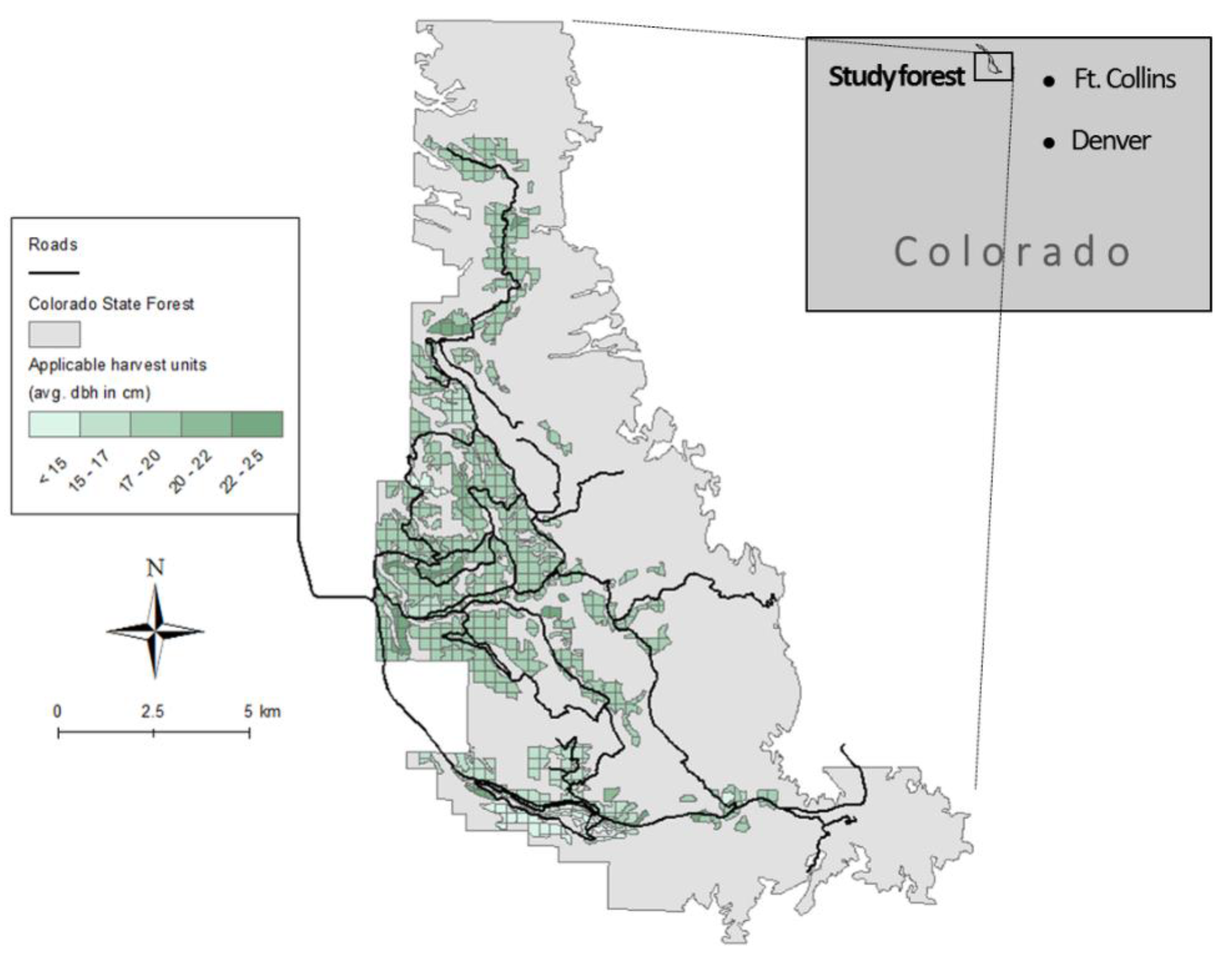
In the Colorado State Forest in northern Colorado, lodgepole pine stands have been heavily impacted by the MPB outbreak since 2008 [68] (Figure 1). Our study site, which is the 3400-ha lodgepole pine forest, has an average mortality rate of 47.3%. It is located on relatively flat terrain with a stand density of 865 trees ha⁻¹ and a basal area of 34.6 m² ha⁻¹. The average tree diameter at breast height (dbh) is 22.4 cm, and the average tree height is 19.6 m. A ground-based clearcut has been a common salvage harvest practice in this area due to the high mortality rate [69]. After accounting for slope and skidding distance, a total of 627 harvest units in average size of 5.4 ha were identified as operationally feasible areas for salvage harvest [70]. Depending on the small-end diameter and defects, three log products, saw logs, post and pole, and firewood, are produced and sold to a timber mill (45 km away) based on oven dry weight. Logging residues for bioenergy alternatives [71] considered in this study include hog fuels (a biomass power plant 238 km away), wood pellets (a pellet plant 45 km away), and biochar (mobile pyrolysis equipment on-site).

The supply chain network of forest salvage utilization consists of a timber supply chain (TSC) and a bioenergy supply chain (BSC), where each operation is associated with a cost and GHG emission. TSC revenues and GHG savings are achieved through end product use (Figure 2). In the TSC, lop-and-scatter (LS) and whole-tree harvesting (WT) are the primary harvesting systems, and employ the same set of equipment. The distinct feature of LS is that delimbers delimb and buck trees to logs at the stump. While processed logs are brought to the landing by a skidder, logging residues are dispersed over the harvest unit and left on the forest floor (i.e., not economical to collect). By comparison, whole trees are transported in WT by a skidder and processed by delimbers at the landing, where slash piles are accumulated as part of timber harvesting [72].

In addition to the two existing systems, a whole-tree harvesting with sorting (WTwS) system can be deployed to include a sorting procedure in the delimbing process of the WT system [73]. WTwS separates and sorts biomass from slash piles, facilitating production of high-quality feedstock. Tree tops left from saw log processing and delimbed small diameter trees can be separated and sorted by size with minimal contamination from dirt. The overall cost of timber harvesting is increased compared to that of WT, but high-value bioenergy products increase revenue.

At completion of the salvage harvest, trees in unharvested units and the scattered logging residues that remain in LS units are left to decay and emit GHG as carbon sources. Forest residues and sorted biomass from WT and WTwS harvested units, respectively, can be further utilized in the BSC for bioenergy production. Pellets and biochar production normally require homogenous sized, less contaminated feedstock, which can be produced through chipping sorted biomass with a chipper. In contrast, forest residues from WT harvest units contain a wide range of woody materials (e.g., tops, limbs and chunks) and high amounts of soil contamination, limiting options for comminution to grinding for low-quality feedstock products (i.e., hog fuels) [74]. For use in pellet or biochar production we assume a screening process is required after grinding to reduce contamination content and improve feedstock quality [75]. After comminution, produced feedstock is transported to the selected bioenergy facility to manufacture bioenergy products. Unutilized forest residues should be burned as part of harvest unit cleanup and disposal management.

Timber harvesting and biomass utilization in the study region are conducted by different stakeholders (i.e., timber and bioenergy producers), and the landowner works separately with TSC and BSC stakeholders. Harvest decisions are made to optimize TSC performance without considering impacts on or from a BSC, despite salvage harvest effects on biomass feedstock amount and form. In addition, biomass utilization affects the residue disposal management.

After the salvage harvest, biomass availability is assessed and managed for bioenergy production to optimize performances of the BSC. Disposal of unutilized biomass residue remains a responsibility of the TSC. This sequential decision-making process is the Sequential scenario that lacks cooperation between the TSC and BSC, neglecting interaction between the two supply chains that may lead to suboptimal outcomes when their performances are combined and evaluated.

We hypothesize that an Integrated scenario, where the TSC and BSC are managed jointly, can utilize the beetle-killed forest resource most efficiently, and may benefit both timber and bioenergy production. This scenario represents a fully communicated and cooperative supply chain network where the landowner works collectively with timber and bioenergy producers to optimize the performance of the overall supply chain of forest products.

3. Methods

3.1. Mathematical Model

We combined multi-objective optimization (MOO) with mixed integer linear programming (MILP) to optimize the economic and environmental objectives of the forest supply chain under the Sequential and Integrated scenarios. The economic objective was measured by net revenues ($NR$) and the environmental objective was measured by the net GHG emission savings ($NS$). Instead of a single solution optimizing both objectives, MOO produces a set of Pareto optimal solutions, where in each solution, one objective cannot be improved without sacrificing the other objective [76]. $NR$ and $NS$ values calculated from the solution set constructed the Pareto front which showed the trade-offs between the two objectives [47]. In model formulation, the Sequential and Integrated scenarios shared the same variables, parameters (

Table 1. Optimization model nomenclature.

Sets
$I$	Set of harvest unit $i$
$S$	Set of harvesting systems $s$
$T$	Set of logging residue treatments $t$
$C$	Set of comminution methods $c$
$L$	Set of log products $l$
$K$	Set of bioenergy feedstocks $k$
$P$	Set of bioenergy products $p$
Parameters
(1) General
$m_{i,l}^{Log}$	Available log product $l$ at harvest unit $i$ in oven dry metric ton (odt)
$m_i^{Res}$	Available logging residues at harvest unit $i$ (odt)
$a_i$	Area of harvest unit $i$ (ha)
$d_i^{Log}$	Distance between harvest unit $i$ and the timber mill (km)
$d_{i,p}^{Feed}$	Distance between harvest unit $i$ and the bioenergy product $p$ facility (km)
$GW{P}_{bio}^{decay}$	GWP factor of biogenic carbon emission from biomass decaying
$GW{P}_{bio}^{burn}$	GWP factor of biogenic carbon emission from biomass burning
(2) Economic
$c_i^{Admin}$	Salvage harvest administration cost ($/ha)
$c_{i,s}^{Log,har}$	Cost of salvage harvest using system $s$ at unit $i$ ($/odt)
$c_l^{Log,trans}$	Transportation cost of log type $l$ ($/odt*km)
$r_l^{Log}$	Revenue of delivered log product $l$ ($/odt)
$c^{Res,burn}$	Cost of burning logging residues on site ($/ha)
$c_c^{Res,com}$	Cost of comminuting logging residues with method $c$ ($/odt)
$c_k^{Feed,trans}$	Transportation cost of residue feedstock $k$ ($/odt*km)
$r_{k,p}^{Feed}$	Revenue of using feedstock $k$ for bioenergy product $p$ ($/odt)
(3) Environmental
$e_{i,s}^{Log,har}$	Greenhouse gas (GHG) emissions of salvage harvest using system $s$ at unit $i$ (kg CO2 eq/odt)
$e_l^{Log,trans}$	Transportation GHG emissions of log type $l$ (kg CO2 eq/odt*km)
$s_l^{Log}$	GHG emission savings of log product $l$ (kg CO2 eq/odt)
$e^{decay}$	GHG emissions o biomass decay on site (kg CO2 eq/odt)
$e^{burn}$	GHG emissions of burning logging residues on site (kg CO2 eq/odt)
$e_c^{Res,com}$	GHG emissions of comminuting logging residues with method $c$ (kg CO2 eq/odt)
$e_k^{Feed,trans}$	Transportation GHG emissions of residue feedstock $k$ (kg CO2 eq/odt*km)
$s_{k,p}^{Feed}$	GHG emission savings of using feedstock $k$ for bioenergy product $p$ (kg CO2 eq/odt)
Decision Variables
(1) Continuous variables
$x_{i,l}^{Log}$	Amount of log type $l$ produced at harvest unit $i$
$x_i^{Res}$	Amount of logging residues produced at harvest unit $i$
$x_{i,k}^{Feed}$	Amount of residue feedstock $k$ produced at harvest unit $i$
$x_{i,k,p}^{Feed}$	Amount of residue feedstock $k$ used to produce bioenergy product $p$ at harvest unit $i$
(2) Integer variables
$y_{i,s}$	Binary:1, if harvest unit $i$ is harvested using system $s$; 0, otherwise
$z_{i,t}$	Binary:1, if logging residues at harvest unit $i$ are processed by treatment $t$; 0, otherwise
$v_{i,c}$	Binary:1, if logging residues at harvest unit $i$ are comminuted by method $c$; 0, otherwise
$u_c$	Binary:1, if comminution method $c$ is used; 0, otherwise

) and constraints, but differed in the solution procedures that simulate the distinctive decision-making processes of the two planning strategies.

Net revenues and net GHG emission savings of the TSC ($N{R}_{TSC}$ and $N{S}_{TSC}$) and BSC ($N{R}_{BSC}$ and $N{S}_{BSC}$) are summarized (Equations (1)–(4)); the results are used to construct objective functions in MOO models of the Sequential and Integrated strategies. $N{R}_{TSC}$ is calculated by using log sale revenues to subtract log stumpage costs, harvesting costs, residue burning costs, and log transportation costs (Equation (1)). Correspondingly, $N{S}_{TSC}$ is calculated by using log product GHG emission savings to subtract harvesting emissions, log transportation emissions, unharvested forest decay emissions, residue decay emissions, and residue burning emissions (Equation (2)). $N{R}_{BSC}$ is calculated by using bioenergy sale revenues to subtract machine move-in costs, residue comminution costs, feedstock transportation costs, and bioenergy product manufacturing costs (Equation (3)). $N{S}_{BSC}$ is calculated by using bioenergy GHG emission savings to subtract GHG emissions from residue comminution, feedstock transportation, bioenergy, and product manufacturing (Equation (4)).

$$\begin{array}{l}N{R}_{TSC}={{\displaystyle \sum }}_{i\in I}{{\displaystyle \sum }}_{l\in L}{x}_{i,l}^{Log}\times r_l^{Log}-{{\displaystyle \sum }}_{i\in I}{a}_i\times c_i^{Admin}-{{\displaystyle \sum }}_{i\in I}{{\displaystyle \sum }}_{s\in S}{{\displaystyle \sum }}_{l\in L}{m}_{i,l}^{Log}\times y_{i,s}\times c_{i,s}^{Log,har}\\ -c^{burn}\ast {{\displaystyle \sum }}_{i\in I}{a}_i\ast z_{i,burn}-{{\displaystyle \sum }}_{i\in I}{{\displaystyle \sum }}_{l\in L}{x}_{i,l}^{Log}\ast d_i^{Log}\ast c_l^{Log,trans}\end{array}$$

(1)

$$\begin{array}{l}N{S}_{TSC}={{\displaystyle \sum }}_{i\in I}{{\displaystyle \sum }}_{l\in L}{x}_{i,l}^{Log}\times s_l^{Log}-{{\displaystyle \sum }}_{i\in I}{{\displaystyle \sum }}_{s\in S}{{\displaystyle \sum }}_{l\in L}{m}_{i,l}^{Log}\times y_{i,s}\times e_{i,s}^{Log,har}\\ -GW{P}_{bio}^{decay}\times e^{decay}\times {{\displaystyle \sum }}_{i\in I}\left(\left({{\displaystyle \sum }}_{l\in L}{m}_{i,l}^{Log}+m_i^{Res}\right)\left(1-{{\displaystyle \sum }}_{s\in S}{y}_{i,s}\right)+m_i^{Res}\times z_{i,decay}\right)\\ -GW{P}_{bio}^{burn}\times e^{burn}\times {{\displaystyle \sum }}_{i\in I}{m}_i^{Res}\times z_{i,burn}-{{\displaystyle \sum }}_{i\in I}{{\displaystyle \sum }}_{l\in L}{x}_{i,l}^{Log}\times d_i^{Log}\times e_l^{Log,trans}\end{array}$$

(2)

$$\begin{array}{l}N{R}_{BSC}={{\displaystyle \sum }}_{i\in I}{{\displaystyle \sum }}_{p\in P}{{\displaystyle \sum }}_{k\in K}{x}_{i,k,p}^{Feed}\times r_{k,p}^{Feed}-u^{Res}\times c^{Move}-{{\displaystyle \sum }}_{i\in I}{{\displaystyle \sum }}_{c\in C}{m}_i^{Res}\times v_{i,c}\times c_c^{Res,com}\\ -{{\displaystyle \sum }}_{i\in I}{{\displaystyle \sum }}_{k\in K}{x}_{i,k}^{Feed}\times d_{i,p}^{Feed}\times c_k^{Feed,trans}\end{array}$$

(3)

$$\begin{array}{l}N{S}_{BSC}={{\displaystyle \sum }}_{i\in I}{{\displaystyle \sum }}_{p\in P}{{\displaystyle \sum }}_{k\in K}{x}_{i,k,p}^{Feed}\times s_{k,p}^{Feed}-u^{Res}\times e^{Move}-{{\displaystyle \sum }}_{i\in I}{{\displaystyle \sum }}_{c\in C}{m}_i^{Res}\times v_{i,c}\times e_c^{Res,com}\\ -{{\displaystyle \sum }}_{i\in I}{{\displaystyle \sum }}_{k\in K}{x}_{i,k}^{Feed}\times d_i^{Feed}\times e_k^{Feed,trans}\end{array}$$

(4)

Each harvest unit $i$ can be harvested only one time by one of the available harvesting systems (Equation (5)). The amount of each log type $l$ produced equals the available amount from that unit if the unit is harvested (Equation (6)).

$${\displaystyle \sum }_{s\in S}{y}_{i,s}\le 1\forall i\in I$$

(5)

$$x_{i,l}^{Log}={\displaystyle \sum }_{s\in S}{y}_{i,s}\times m_{i,l}^{Log}\forall l\in L,i\in I$$

(6)

If a unit is harvested by the LS system, logging residues are left on-site to decay (Equation (7)). If logging residues are burned, the unit should be harvested by the WT system (Equation (8)). If logging residues are used for bioenergy production, the unit should be either harvested by the WT or WTwS system (Equation (9)).

$$z_{i,decay}=y_{i,ls}\forall i\in I$$

(7)

$$z_{i,burn}\le y_{i,wt}\forall i\in I$$

(8)

$$z_{i,use}\le y_{i,wt}+y_{i,wtws}\forall i\in I$$

(9)

If no logging residues on each harvest unit are utilized, none of the comminution methods should be chosen. Otherwise, one comminution method should be chosen to process logging residues (Equation (11)). Specifically, the chipping method can only be used at units harvested by the WTwS system, while grinding only or grinding with screening can be used at units harvested by the WT system (Equations (11) and (12)). For the entire forest site, if logging residues from any unit are processed by a comminution equipment, this equipment need to be deployed to the site (Equation (13)).

$${\displaystyle \sum }_{c\in C}{v}_{i,c}=z_{i,use}\forall i\in I$$

(10)

$$v_{i,chip}=y_{i,wtws}\forall i\in I$$

(11)

$$v_{i,grind}+v_{i,gws}\le y_{i,wt}\forall i\in I$$

(12)

$$\left|I\right|\ast u_c\ge {\displaystyle \sum }_{i\in I}{v}_{i,c}\forall c\in C$$

(13)

Low-quality feedstock is produced from the comminution process, e.g., grinding operation and high-quality feedstock is produced from chipping or grinding with screening operations (Equations (14) and (15)). The total amount of feedstock used for all bioenergy products equals the available feedstock in each type (Equation (16)).

$$x_{i,low}^{Feed}=m_i^{Res}\times v_{i,grind}\forall i\in I$$

(14)

$$x_{i,high}^{Feed}=m_i^{Res}\times \left(v_{i,gws}+v_{i,chip}\right)\forall i\in I$$

(15)

$$x_{i,k}^{Feed}={\displaystyle \sum }_{p\in P}{x}_{i,k,p}^{Feed}\forall k\in K,i\in I$$

(16)

Lastly, Equations (17) and (18) show variable type constraints for continuous and binary variables for the MOO model.

$$x_{i,l}^{Log},x_i^{Res},x_{i,k,p}^{Feed},x_{i,k}^{Feed}\in R_{+}\forall l\in L,k\in K,i\in I,p\in P$$

(17)

$$y_{i,s},z_{i,t},u_c,v_{i,c}\in \left\{0,1\right\}\forall t\in T,c\in C,i\in I$$

(18)

We compared the Sequential and Integrated scenarios in managing the supply chain of salvaging beetle-killed stands in the Colorado State Forest. The Sequential scenario was simulated by sequentially optimizing the TSC and BSC in two steps: an evaluation of their individual performances, and then combining the performance of the two solutions for an overall solution quality (Figure 3). The Integrated scenario was simulated by simultaneously optimizing the overall performance of the two supply chains (Figure 4). Details of the modeling and evaluation procedures follow.

3.1.1. Sequential Scenario

Step 1: This step mimics the process where harvesting operations at the TSC are conducted without consideration for residue utilization at the BSC. First, the TSC MOO model is solved with objective functions to maximize $N{R}_{TSC}^{\prime }$ and $N{S}_{TSC}^{\prime }$ (Equations (19) and (20)), subject to constraints in Equations (5)–(7),(17),(18) and (21)–(24). $N{R}_{TSC}^{\prime }$ and $N{S}_{TSC}^{\prime }$ are not the final TSC net revenues and net GHG emission savings. They are estimated values where logging residues from all WT harvested units are to be burnt. Due to lack of cooperation between the TSC and BSC, when the infested forest is managed for salvage harvest, it is unknown whether logging residues from WT harvested units are to be used for bioenergy production or not. $N{R}_{TSC}^{\prime }$, $N{S}_{TSC}^{\prime }$, and $z_{i,burn}^{\prime }$ are used to conservatively estimate TSC performances where piled logging residues are treated as wastes (Equation (23)), and account for costs and GHG emissions associated with burning. In the absence of cooperation with bioenergy production, timber production would not use WTwS system for salvage harvest (Equation (24)) because it is always more expensive than the WT system.

The outputs of TSC MOO model are solutions for timber production showing trade-offs between $N{R}_{TSC}^{\prime }$ and $N{S}_{TSC}^{\prime }$. For each solution, harvesting decisions are used as inputs to the BSC MOO model, indicating availabilities of logging residues at harvest units.

$$Economicobjective:MaximizeN{R}_{TSC}^{\prime }$$

(19)

$$Environmentalobjective:MaximizeN{S}_{TSC}^{\prime }$$

(20)

where

$$\begin{array}{l}N{R}_{TSC}^{\prime }={{\displaystyle \sum }}_{i\in I}{{\displaystyle \sum }}_{l\in L}{x}_{i,l}^{Log}\times r_l^{Log}-{{\displaystyle \sum }}_{i\in I}{a}_i\times c_i^{Admin}-{{\displaystyle \sum }}_{i\in I}{{\displaystyle \sum }}_{s\in S}{{\displaystyle \sum }}_{l\in L}{m}_{i,l}^{Log}\times y_{i,s}\times c_{i,s}^{Log,har}\\ -c^{burn}\times {{\displaystyle \sum }}_{i\in I}{a}_i\times z_{i,burn}^{\prime }-{{\displaystyle \sum }}_{i\in I}{{\displaystyle \sum }}_{l\in L}{x}_{i,l}^{Log}\times d_i^{Log}\times c_l^{Log,trans}\end{array}$$

(21)

$$\begin{array}{l}N{S}_{TSC}={{\displaystyle \sum }}_{i\in I}{{\displaystyle \sum }}_{l\in L}{x}_{i,l}^{Log}\times s_l^{Log}-{{\displaystyle \sum }}_{i\in I}{{\displaystyle \sum }}_{s\in S}{{\displaystyle \sum }}_{l\in L}{m}_{i,l}^{Log}\times y_{i,s}\times e_{i,s}^{Log,har}\\ -GW{P}_{bio}^{decay}\times e^{decay}\times {{\displaystyle \sum }}_{i\in I}\begin{array}{c}\left(\left({{\displaystyle \sum }}_{l\in L}{m}_{i,l}^{Log}+m_i^{Res}\right)\left(1-{{\displaystyle \sum }}_{s\in S}{y}_{i,s}\right)+m_i^{Res}\times z_{i,decay}\right)\end{array}\\ -GW{P}_{bio}^{burn}\times e^{burn}\times {{\displaystyle \sum }}_{i\in I}{m}_i^{Res}\times z_{i,burn}^{\prime }-{{\displaystyle \sum }}_{i\in I}{{\displaystyle \sum }}_{l\in L}{x}_{i,l}^{Log}\times d_i^{Log}\times e_l^{Log,trans}\end{array}$$

(22)

$$z_{i,burn}^{\prime }=y_{i,wt}\forall i\in I$$

(23)

$$y_{i,wtws}=0\forall i\in I$$

(24)

Step 2: This step mimics the process of assessing availabilities of logging residues post-harvest, determination by the landowner whether to process residues for bioenergy production, what bioenergy pathway to choose, and how much feedstock to produce. Corresponding to each solution from the TSC MOO model, the BSC MOO model is solved with objective functions to maximize $N{R}_{BSC}$ and $N{S}_{BSC}$ (Equations (25) and (26)), subject to constraints in Equations (3),(4) and (8)–(18). In the BSC MOO model, $y_{i,wt}$ and $y_{i,wtws}$ in Equations (8) and (9) are not variables. They are input values read from the TSC solution. The outputs of the BSC MOO model are solutions for bioenergy production showing trade-offs between $N{R}_{BSC}$ and $N{S}_{BSC}$ based on the residue availability from the input TSC solution. Because each TSC solution represents a new situation of residue availability, a new Pareto front is generated in the BSC MOO model.

$$Economicobjective:MaximizeN{R}_{BSC}$$

(25)

$$Environmentalobjective:MaximizeN{S}_{BSC}$$

(26)

Step 3: Based on timber production and biomass utilization decisions made from Steps 1 and 2, $N{R}_{TSC}$ and $N{S}_{TSC}$ (Equations (1) and (2) are calculated and combined with $N{R}_{BSC}$ and $N{S}_{BSC}$ to obtain $N{R}_{FSC}$ and $N{S}_{FSC}$ (Equations (27) and (28). In this step, every Step 1 TSC solution corresponds to a Step 2 BSC Pareto solution set.

$$N{R}_{FSC}=N{R}_{TSC}+N{R}_{BSC}$$

(27)

$$N{S}_{FSC}=N{S}_{TSC}+N{S}_{BSC}$$

(28)

3.1.2. Integrated Scenario

The integrated forest supply chain (FSC) MOO model is solved with objective functions to maximize $N{R}_{FSC}$ and $N{S}_{FSC}$ (Equations (29) and (30)), subject to constraints Equations (1), (18), (27) and (28). This scenario mimics the process that timber and bioenergy production are jointly managed during the decision-making process to optimize the overall economic and environmental performances of the forest supply chain. The outputs of the FSC MOO model are solutions for timber and bioenergy production showing trade-offs between $N{R}_{FSC}$ and $N{S}_{FSC}$.

$$Economicobjective:MaximizeN{R}_{FSC}$$

(29)

$$Environmentalobjective:MaximizeN{S}_{FSC}$$

(30)

3.2. Solution Procedure

In order to solve MOO models, we applied the augmented ε-constraint (AUGMECON) method [77], which was developed based on the widely used ε-constraint method [76]. During the solution process, a MOO model is first reformulated as single objective problems and solved to obtain the bounds of each objective. Then, one objective is selected and the others are transformed into additional constraints. The new single-objective optimization problem is solved iteratively, where in each iteration the right-hand side of an objective converted constraint is changed with a user-specified step-size of ε value. The AUGMECON method improves the ε-constraint method in the sense that it uses lexicographic optimization to identify objective bounds. Slack variables are added to objective converted constraints and the final objective function to avoid the production of weakly Pareto optimal solutions [77].

In our bi-objective MOO models, after identifying bounds of each objective through single objective optimization, the environmental objective was converted to the additional ε-constraint, and the economic objective was used as the objective function during the iterative optimization process. In the Sequential scenario, the TSC MOO model in Step 1 consisted of 2526 constraints, 3135 binary variables, and 1896 continuous variables, and the BSC MOO model in Step 2 consisted of 4413 constraints, 3766 binary variables, and 1896 continuous variables. A set of 50 Pareto-optimal points was generated from the TSC MOO model and corresponding to each TSC solution a set of three Pareto-optimal points was generated in the BSC MOO model.

In the Integrated scenario, the FSC MOO model consisted 6942 constraints, 5647 binary variables, and 3794 continuous variables, and a set of 50 Pareto-optimal points was generated. All MOO models were formulated in Python 2.7 and solved by the MIP solver CPLEX 12.6.3 on a computer with an Intel 3.40 GHz processor and 16 GB memory. Solution time for the Sequential and Integrated scenarios totaled 264 and 629 seconds, respectively.

We used 0.1 and 0.32 for $GW{P}_{bio}^{decay}$ and $GW{P}_{bio}^{burn}$ to discount the global warming potential [56] of biogenic carbon relative to fossil carbon [78]. Other process parameters and product data used in MOO models are provided in

Table 2. Forest production process parameters.

Unit Process	Criteria	Value	Assumptions and References
Timber Harvesting
Administration	Cost	$494.21/ha	Sale preparation, environmental analysis, and harvest monitoring costs at $200/acre [79].
Salvage Harvest	Cost	$21.51–122.66/odt	Harvesting costs and GHG emissions for each system at each unit are estimated based on She et al. [69].
	Emission	9.74–55.90 kg CO2-eq/odt
Residue Treatment
Chipping	Cost	$18.14/odt	A chipper processes logging residues [80,81].
	Emission	12.14 kg CO2-eq/odt
Grinding	Cost	$/22.81odt	A grinder processes clearcut roundwood logging residues without screening [75].
	Emission	16.19 kg CO2-eq/odt
Grinding with Screening	Cost	$48.45/odt	A grinder processes clearcut roundwood logging residues with screening [75].
	Emission	35.81 kg CO2-eq/odt
Burn	Cost	$200/ha	Burning logging residues on site [82,83].
	Emission	1740 kg CO2-eq/odt
Decay	Emission	1580 kg CO2-eq/odt	Scattered residues decay on forest floor [83].
Residue Transportation
Log	Cost	$0.1735/odt*km	Two-way transportation with log truck payload of 26.7 t. Cost is $2.52/mile and fuel economy is 5.1 mile/gallon [84].
	Emission	0.1695 kg CO2-eq/odt*km
Feedstock	Cost	$0.2038/odt*km	Two-way transportation with chip van payload of 22.7 t. Cost is $0.2038/km and fuel economy is 1.98 km/L [85,86].
	Emission	0.2183 kg CO2-eq/odt*km

and

Table 3. Timber and bioenergy product details.

Product	Criteria	Value	Assumptions and References
Timber
Saw Log	Revenue	$81.53/odt	Lumber has a recovery ratio of 0.46 [87] and substitutes steel stud [19].
	Savings *	1125.12 kg CO2-eq/odt
Post and Pole	Revenue	$58.70/odt	Pole is used as fences and stores carbon during service life [19].
	Savings	705.13 kg CO2-eq/odt
Firewood	Revenue	$48.92/odt	Firewood is combusted in a fireplace for domestic heating, substituting natural gas [88].
	Savings	389.31 kg CO2-eq/odt
Residue Utilization
Low-Quality Feedstock (hog fuels)	Revenue	$55.10/odt	Hog fuel combusted in a boiler to generate electricity, substituting coal [86].
	Savings	1107.23 kg CO2-eq/odt
High-Quality Feedstock (pellets)	Revenue	$70.00/odt	Pellet combusted in a pellet stove for domestic heating, substituting natural gas [88].
	Savings	203.17 kg CO2-eq/odt
High-quality Feedstock (biochar and syngas)	Revenue	$43.43/odt	Pyrolysis outputs contain 17.5% biochar and 82.5% syngas [89], which are used as soil amendments and to generate electricity, respectively.
	Savings	983.72 kg CO2-eq/odt

* Greenhouse gas emission savings.

. The detailed estimation process of all parameters can be found in Appendix A.

4. Results

4.1. Salvage Harvest and Residue Treatment in the Sequential Scenario

In the Sequential scenario, TSC solutions are sorted (x-axis) according to the environmental objective (i.e., $N{S}_{TSC}^{\prime }$) in the TSC MOO model (Figure 5). Only LS and WT systems are used for salvage harvesting in all TSC MOO model solutions and logging residues are either decayed, burnt, or used for hog fuels in BSC MOO model solutions. The maximum $N{R}_{TSC}^{\prime }$ solution leads to 919.35 ha of forest area being harvested (93% by LS and 7% by WT), resulting in a production of 84.76 thousand (M) odt of timber products (63% saw logs, 22% post and pole, and 15% firewood).

When the TSC MOO model focuses more on the environmental objective, a higher $N{S}_{TSC}^{\prime }$ needs to be satisfied as the additional ε-constraint during the optimization process. LS harvested areas increase while WT harvested areas remain relatively constant. These WT areas eventually also switch to the LS system gradually, as the environmental objective further increases and the entire forest stand is harvested by LS where the maximum $N{S}_{TSC}^{\prime }$ solution is obtained at 203.67 M odt of timber products (52% saw logs, 27% post and pole, and 20% firewood) produced from 3070.43 ha of harvested forest area.

As for bioenergy production, the maximum $N{R}_{TSC}^{\prime }$ solution results in 12.89 odt of residues from LS harvested units that are left to decay, and 1.07 odt of residues from WT harvested units that are available for further utilization. The residues from WT units then become inputs to the BSC MOO model. The maximum $N{R}_{BSC}$ solution results in all residues being burnt on site, because no bioenergy pathway is economically feasible given the form and amount of available logging residues. The maximum $N{S}_{BSC}$ solution results in all residues being utilized for hog fuels because they are the most GHG emission-saving bioenergy product. A compromise solution, achieving the average $N{S}_{BSC}$ of the previous two solutions, results in 0.53 odt of residues being burnt, and 0.54 odt residues being utilized.

As the TSC MOO model focuses more on the environmental objective, residue decay amount increases, while residue available for bioenergy production remains relatively constant. Depending on the ε-constraint in the BSC MOO model, residues are fully burnt, fully utilized for hog fuels, and partially burnt and partially utilized in the maximum $N{R}_{BSC}$, the maximum $N{S}_{BSC}$, and the compromise solutions, respectively. Corresponding to the maximum $N{S}_{TSC}^{\prime }$ solution, no residues are available for further utilization, and all BSC solutions lead to zero burning or hog fuel production.

4.2. Salvage Harvest and Residue Treatment in the Integrated Scenario

In the Integrated scenario, FSC solutions are sorted (x-axis) according to the environmental objective (i.e., $N{S}_{FSC}$) in the FSC MOO model (Figure 6). The maximum $N{R}_{FSC}$ solution leads to 1375.45 ha harvested (24% by LS, 57% by WT, and 19% by WTwS) and 109.78 M odt of timber products produced (59% saw logs, 24% post and pole, and 17% firewood). As the optimization shifts from maximizing $N{R}_{FSC}$ to maximizing $N{S}_{FSC}$, a higher $N{S}_{FSC}$ needs to be satisfied as the additional ε-constraint during the optimization process. As a result, LS harvested areas increase while WTwS harvested areas remain constant at first; but, both change to the WT system when the $N{S}_{FSC}$ is high enough. WT harvested areas increase throughout the whole process, either from harvesting previously unharvested areas or switching the harvest system at previously LS or WTwS harvested areas, until WT takes over the entire forest area of 3070.43 ha in the maximum $N{S}_{FSC}$ solution.

For residue treatment at the BSC, no residue burning operations are ever chosen. The maximum $N{R}_{FSC}$ solution leads to 4.97 M odt of residues being left to decay and 13.30 M odt being used for pellet production (for comminution, 3.96 M odt are chipped and 9.34 M odt are ground and screened). As the optimization focuses more on maximizing $N{S}_{FSC}$, residue decay amount increases first then decreases to zero, following the trend of LS harvested areas. Residue utilization amount increases because the WT system is applied to larger areas, providing greater amounts of logging residues available for bioenergy production. There is a transition in the bioenergy production from pellets (the most profitable product) to hog fuels (the most GHG emission saving product). The maximum $N{S}_{FSC}$ solution utilizes 34.68 M odt of residues for hog fuel production.

4.3. Net Revenues and GHG Emission Savings in the Sequential and Integrated Scenarios

The Sequential and Integrated scenarios produce distinctive results when either the economic or environmental objective is used for optimization (

Table 4. Single objective optimization under the Sequential and Integrated scenarios. MM = million.

Scenario	Sequential		Integrated	Sequential		Integrated
Solution	$\mathit{M}\mathit{a}\mathit{x}\mathit{N}{\mathit{R}}_{\mathit{T}\mathit{S}\mathit{C}}^{\prime }$		$\mathit{M}\mathit{a}\mathit{x}\mathit{N}{\mathit{R}}_{\mathit{F}\mathit{S}\mathit{C}}$	$\mathit{M}\mathit{a}\mathit{x}\mathit{N}{\mathit{S}}_{\mathit{T}\mathit{S}\mathit{C}}^{\prime }$		$\mathit{M}\mathit{a}\mathit{x}\mathit{N}{\mathit{S}}_{\mathit{F}\mathit{S}\mathit{C}}$
	$\mathit{M}\mathit{a}\mathit{x}\mathit{N}{\mathit{R}}_{\mathit{B}\mathit{S}\mathit{C}}$	$\mathit{M}\mathit{a}\mathit{x}\mathit{N}{\mathit{S}}_{\mathit{B}\mathit{S}\mathit{C}}$		$\mathit{M}\mathit{a}\mathit{x}\mathit{N}{\mathit{R}}_{\mathit{B}\mathit{S}\mathit{C}}$	$\mathit{M}\mathit{a}\mathit{x}\mathit{N}{\mathit{S}}_{\mathit{B}\mathit{S}\mathit{C}}$
$N{R}_{TSC}$ (MM $)	1.29	1.31	1.18	0.11	0.11	−0.32
$N{R}_{BSC}$ (MM $)	0	−0.03	0.27	0	0	−0.53
$N{R}_{FSC}$ (MM $)	1.29	1.28	1.45	0.11	0.11	−0.85
$N{S}_{TSC}$ (MM t CO2-eq)	73.36	73.96	108.21	224.76	224.76	230.42
$N{S}_{BSC}$ (MM t CO2-eq)	0	1.11	2.21	0	0	36.08
$N{S}_{FSC}$ (MM t CO2-eq)	73.36	75.07	110.42	224.76	224.76	266.50

). In the Sequential scenario, maximizing $N{R}_{TSC}^{\prime }$ in the TSC MOO model and $N{R}_{BSC}$ in the BSC MOO model generates 1.29 and 0 million (MM) dollar in net revenues with 73.36 and 0 MM t CO₂-eq GHG emission savings from the TSC and BSC, respectively. Maximizing $N{R}_{TSC}^{\prime }$ from the TSC and $N{S}_{BSC}$ from the BSC generates 1.31 and −0.03 million (MM) dollars in net revenues with 73.96 and 1.11 MM t CO₂-eq GHG emission savings from the TSC and BSC, respectively.

The increased $N{R}_{TSC}$ and decreased $N{R}_{BSC}$ in the second solution are shown because the TSC does not need to burn logging residues on-site, and the BSC has to utilize them. When performances of TSC and BSC are combined, $N{R}_{FSC}$ and $N{S}_{FSC}$ of these two solutions are 1.29 MM dollars with 73.36 MM t CO₂-eq GHG emission savings and 1.28 MM dollars with 75.07 MM t CO₂-eq GHG emission savings. In the Integrated scenario, maximizing $N{R}_{FSC}$ results in $N{R}_{TSC}$, $N{R}_{BSC}$, and $N{R}_{FSC}$ being 1.18, 0.27, and 1.45 MM dollars, respectively, and $N{S}_{TSC}$, $N{S}_{BSC}$, $N{S}_{FSC}$ being 108.21, 2.21, and 110.42 MM t CO₂-eq GHG, respectively.

Maximizing $N{S}_{TSC}^{\prime }$ in the TSC MOO model in the Sequential scenario results in 0.11 MM dollars in net revenues with 224.76 MM t CO₂-eq GHG emission savings at the TSC. This corresponds to the solution where the entire forest is harvested by the LS system and no logging residues are available for the BSC to utilize. As a result, maximizing $N{R}_{BSC}$ or $N{S}_{BSC}$ leads to the same outputs, where 0 net revenues and 0 GHG emission savings are achieved at the BSC. In the Integrated scenario, maximizing $N{S}_{FSC}$ results in $N{R}_{TSC}$, $N{R}_{BSC}$, and $N{R}_{FSC}$ values being −0.32, −0.53, and −0.85 MM dollars, respectively, and $N{S}_{TSC}$, $N{S}_{BSC}$, and $N{S}_{FSC}$ values being 230.42, 36.08, and 266.50 MM t CO₂-eq GHG, respectively.

In the Sequential scenario, given the same TSC solution, the three BSC solutions only show small differences due to the small amount of residue available for bioenergy production (Figure 7). After combining TSC and BSC performances, the resulting three curves are not very distinct in terms of trade-offs between $N{R}_{FSC}$ and $N{S}_{FSC}$. The Pareto front from the Integrated scenario lies above all curves of the Sequential scenario and provides a wider range of trade-offs between $N{R}_{FSC}$ and $N{S}_{FSC}$. For both scenarios, trade-off curves have negative slopes because the two objectives, $N{R}_{FSC}$ and $N{S}_{FSC}$, are conflicting and cannot be improved at the same time.

When the optimization emphasizes the economic objective, a small compromise in $N{R}_{FSC}$ causes significant improvements in $N{S}_{FSC}$. When the optimization is skewed toward the environmental objective, a much greater sacrifice has to be made in $N{R}_{FSC}$ to obtain a small increase in $N{S}_{FSC}$.

5. Discussion

5.1. Fully Economic-Oriented or Environmental-Oriented Solutions

When MOO models are fully economic-oriented (i.e., maximizing $N{R}_{TSC}^{\prime }$ and $N{R}_{BSC}$ in the Sequential scenario and maximizing $N{R}_{FSC}$ in the Integrated scenario), 49.6% more forest areas (i.e., 456.1 ha) are harvested in the Integrated scenario (Figure 5 and Figure 6), generating 12.3% more $N{R}_{FSC}$ (i.e., 0.16 MM dollars) and 50.5% more $N{S}_{FSC}$ (i.e., 37.06 MM t CO₂-eq) than those in the Sequential scenario (Table 4). The distribution of the produced log products shows that the additional harvested areas are composed of the harvest units with lower saw log proportion, indicating cooperation between the TSC and BSC results in the salvage harvest being economically feasible in larger harvest units. When MOO models are fully environmental-oriented (i.e., maximizing $N{S}_{TSC}^{\prime }$ and $N{S}_{BSC}$ in the Sequential scenario and maximizing $N{S}_{FSC}$ in the Integrated scenario), the entire beetle-infested forest is harvested under both scenarios. The Integrated scenario utilizes all logging residues for hog fuel production and achieves 18.6% greater $N{S}_{FSC}$ (i.e., 41.74 MM t CO₂-eq), but results in a loss of 0.96 MM $ in $N{R}_{FSC}$ compared to the Sequential scenario solution.

While the fully environmental-oriented solutions may be economically prohibitive for practical implementations, operations following fully economic-oriented solutions are commonly practiced. In the current salvage harvest in Colorado State Forest, timber salvage and residue utilization are managed by the landowner as two separate operations with economic feasibility being the main consideration for either operation, similar to the fully economic-oriented solution in the Sequential scenario. During the salvage harvest, although the WT system can be less expensive than the LS system when the skidding distance is short, the extra burning cost disfavors its application [68]. Without knowing whether residues are to be utilized, the landowner has preferred the LS system for salvage harvest, because it is easy to implement and more economical for slash management [90]. This suboptimal decision may lead to higher harvesting cost at the TSC and a small amount of residues in undesirable form for bioenergy production in the BSC. Consequently, only a small portion of infested forests are harvested, and no bioenergy products are produced from logging residues.

In this study, the fully economic-oriented solutions clearly demonstrate that the Integrated scenario outperforms the Sequential scenario in both $N{R}_{FSC}$ and $N{S}_{FSC}$. Our analysis confirms that the BSC generates net revenues and GHG emission savings at a much smaller scale than the TSC. However, timber production should still be managed together with bioenergy production to prepare residues in a desirable form for bioenergy production and avoid on-site pile burning. The joint management in the TSC and BSC, through an integrated decision-making process, results in quite distinct decisions in salvage harvest and residue utilization (Figure 6) compared to those in the Sequential scenario (Figure 5). The integrated solution promotes more efficient use of logging residues and benefits the landowner both economically and environmentally.

5.2. Trade-Offs between $N{R}_{FSC}$ and $N{S}_{FSC}$

As the ε-constraint sets a higher environmental objective, harvest areas increase in both scenarios, but the difference in harvest system selection is apparent. The Sequential scenario favors the LS system to avoid residue burning (Figure 5), while the Integrated scenario favors WT and WTwS systems to facilitate bioenergy production (Figure 6). As a result, logging residue availability and utilization is limited in the Sequential scenario (Figure 5), whereas the utilized residue amount increases and bioenergy production switches from the most profitable product (i.e., pellets) to the most GHG-saving product (i.e., hog fuels) in the Integrated scenario.

In terms of trade-offs between $N{R}_{FSC}$ and $N{S}_{FSC}$ (Figure 7), all three curves of the Sequential scenario are completely dominated [91] by the Pareto front of the Integrated scenario. For any solution from the Sequential scenario, there always exists at least one solution from the Integrated scenario that outperforms in both $N{R}_{FSC}$ and $N{S}_{FSC}$. Therefore, the Integrated scenario has proven strictly better than the Sequential scenario.

5.3. Impact of Carbon Accounting on Trade-Offs Between $N{R}_{FSC}$ and $N{S}_{FSC}$

Carbon accounting has a strong influence on evaluating the GHG emission savings of timber and bioenergy products. Because the estimation of carbon sequestration (e.g., biomass growth, soil carbon pool, land use changes) is site-specific, the exact values of GHG emission savings provided by woody products are often uncertain [59]. The assumption of carbon neutrality of all biogenic sources appears to be inappropriate and has raised debate especially on how to account for carbon emissions from burning woody materials [61,67,88].

We explored different $GW{P}_{bio}^{burn}$ values when solving the MOO models to assess the influence of carbon accounting on trade-offs between $N{R}_{FSC}$ and $N{S}_{FSC}$ (Figure 8). GHG emissions from biomass burning are treated equivalently to biomass decay emissions when $GW{P}_{bio}^{burn}$ equals 0.1, and equivalently to fossil carbon when $GW{P}_{bio}^{burn}$ equals 1.0. The results show a significant difference in the Pareto fronts when different $GW{P}_{bio}^{burn}$ values are used for GHG accounting. As $GW{P}_{bio}^{burn}$ increases from 0.1 to 1, the maximum $N{R}_{FSC}$ in the Sequential and Integrated scenarios do not change because economic features of timber and bioenergy products remain the same. However, the maximum $N{S}_{FSC}$ of the two scenarios decrease drastically because carbon benefits of timber and bioenergy products are considered much smaller. Trade-offs between $N{R}_{FSC}$ and $N{S}_{FSC}$ become more apparent with low $GW{P}_{bio}^{burn}$ cases than high $GW{P}_{bio}^{burn}$ cases.

Greater economic compromises should be made to obtain the same environmental improvement with high $GW{P}_{bio}^{burn}$. In addition, the $GW{P}_{bio}^{burn}$ also affects the bioenergy product produced. If $GW{P}_{bio}^{burn}$ equals 0.1 or 0.32, i.e., burning woody biomass has small global warming potential relative to emitting fossil carbon, substituting coal with hog fuels is the most GHG emission saving pathway, and is selected to achieve high $N{S}_{FSC}$. In contrast, if $GW{P}_{bio}^{burn}$ equals 1, i.e, there is no difference between burning woody biomass and emitting fossil carbon, producing biochar to preserve carbon is the most GHG emission saving pathway, and is selected to achieve high $N{S}_{FSC}$.

Given the same $GW{P}_{bio}^{burn}$ value, the Integrated scenario always outcompetes the Sequential scenario, shown by the dominating relationship of the two trade-off curves [91]. This is because cooperation between the TSC and BSC in the Integrated scenario avoids residue burning and facilitates bioenergy production, regardless of the $GW{P}_{bio}^{burn}$ value. However, as $GW{P}_{bio}^{burn}$ increases from 0.1 to 1, the gap shrinks between trade-off curves, indicating a decreasing difference in trade-offs between $N{R}_{FSC}$ and $N{S}_{FSC}$ of the two scenarios. This is because higher $GW{P}_{bio}^{burn}$ decreases the amount of carbon benefits of timber and bioenergy products; therefore, the gain in $N{S}_{FSC}$ is not as significant as in the low $GW{P}_{bio}^{burn}$ case.

5.4. Study Limitations and Practical Implications

The mathematical programming models presented in this study are deterministic, and the production processes were modeled based on the average performance data, which can widely vary in practice depending on vegetation, terrain and operational conditions [92]. In addition, as components of a supply chain are often interdependent, a change in performance of one component may cause a series of effects along the supply chain, affecting the overall system performance [93,94]. Our models did not account for these variations of system performance. Our models also did not consider any temporal changes in beetle-killed stands such as log degradation and possible harvest cost increase over time [3,23,95,96]. Uncertainties and information gaps still remain on how MPB-infested stands change over time and how these changes affect salvage operations and product recovery. Our models can be refined when more information becomes available on dynamic variations in system performance and temporal changes in beetle-killed stands.

Despite the model limitations, our comparison between the Sequential and Integrated scenarios highlights the differences in supply chain performances of the two scenarios and potential benefits from integrating bioenergy production with timber harvest when salvage utilizing beetle-killed forests. Our study analyzes different management strategies focusing on the effective use of forest resources post natural disturbances with existing infrastructure and locally available facilities. This could be particularly helpful for small to medium scale forest decision-makers and stakeholders who are unable to make large capital investments but seek for opportunity for an efficiency gain in timber and bioenergy production. Case-specific data and practical management constraints, such as opening size limit, should be considered, when applicable, for a successful implementation of the Integrated scenario in real-world applications.

6. Conclusions

Salvage harvesting of beetle-kill trees in northern Colorado provides an opportunity to mitigate economic losses and produce carbon benefits. Our multi-objective optimization analysis shows that the Integrated scenario representing joint management for timber and bioenergy production can enhance the economic feasibility of forest salvage utilization, while simultaneously increasing GHG emission savings. When the optimization is fully economic-oriented, the Integrated scenario tends to harvest more forest areas and produce more bioenergy products than the Sequential scenario, generating greater total net revenues and GHG emission savings from timber and bioenergy production. A comparison of Pareto fronts indicates the Integrated scenario offers more efficient trade-offs between $N{R}_{FSC}$ and $N{S}_{FSC}$ and always outperforms the Sequential scenario in both objectives, regardless of the carbon accounting scheme. From the landowner’s perspective, the Integrated scenario generates more profits and requires less monetary sacrifice than the Sequential scenario for the same GHG emission savings.

References

1. Barry, P.; Duda, J.; Garrison, K.; Lockwood, R.; Mason, L.; Matthews, S.; Mueller, K.; Reader, T.; West, D. 2017 Report on the Health of Colorado’s Forests: Meeting the Challenge of Dead and At-Risk Trees; Colorado State Forest Service: Fort Collins, CO, USA, 2018; p. 28. [Google Scholar]
2. Duda, J.; Lockwood, R.; Mason, L.; Matthews, S.; Mueller, K.; West, D. 2015 Report on the Health of Colorado’s Forests: 15 Years of Change; Colorado State Forest Service: Fort Collins, CO, USA, 2016; p. 32. [Google Scholar]
3. Lewis, K.; Thompson, D. Degradation of Wood in Standing Lodgepole Pine Killed by Mountain Pine Beetle. Wood Fiber Sci. 2011, 43, 130–142. [Google Scholar]
4. Romme, W.H.; Knight, D.H.; Yavitt, J.B. Mountain Pine Beetle Outbreaks in the Rocky Mountains: Regulators of Primary Productivity? Am. Nat. 1986, 127, 484–494. [Google Scholar] [CrossRef]
5. Corbett, L.J.; Withey, P.; Lantz, V.A.; Ochuodho, T.O. The economic impact of the mountain pine beetle infestation in British Columbia: Provincial estimates from a CGE analysis. Forestry 2015, 89, 100–105. [Google Scholar] [CrossRef]
6. Arnberger, A.; Ebenberger, M.; Schneider, I.E.; Cottrell, S.; Schlueter, A.C.; von Ruschkowski, E.; Venette, R.C.; Snyder, S.A.; Gobster, P.H. Visitor Preferences for Visual Changes in Bark Beetle-Impacted Forest Recreation Settings in the United States and Germany. Environ. Manag. 2018, 61, 209–223. [Google Scholar] [CrossRef] [PubMed]
7. Rosenberger, R.S.; Bell, L.A.; Champ, P.A.; White, E.M. Estimating the economic value of recreation losses in Rocky Mountain National Park due to a mountain pine beetle outbreak. West. Econ. Forum. 2013, 12, 31–39. [Google Scholar]
8. Price, J.I.; McCollum, D.W.; Berrens, R.P. Insect infestation and residential property values: A hedonic analysis of the mountain pine beetle epidemic. For. Policy Econ. 2010, 12, 415–422. [Google Scholar] [CrossRef]
9. Dhar, A.; Parrott, L.; Heckbert, S. Consequences of mountain pine beetle outbreak on forest ecosystem services in western Canada. Can. J. For. Res. 2016, 46, 987–999. [Google Scholar] [CrossRef] [Green Version]
10. Saab, V.A.; Latif, Q.S.; Rowland, M.M.; Johnson, T.N.; Chalfoun, A.D.; Buskirk, S.W.; Heyward, J.E.; Dresser, M.A. Ecological consequences of mountain pine beetle outbreaks for wildlife in western North American forests. For. Sci. 2014, 60, 539–559. [Google Scholar] [CrossRef]
11. Hicke, J.A.; Johnson, M.C.; Hayes, J.L.; Preisler, H.K. Effects of bark beetle-caused tree mortality on wildfire. For. Ecol. Manag. 2012, 271, 81–90. [Google Scholar] [CrossRef]
12. Harvey, B.J.; Donato, D.C.; Turner, M.G. Recent mountain pine beetle outbreaks, wildfire severity, and postfire tree regeneration in the US Northern Rockies. Proc. Natl. Acad. Sci. USA 2014, 111, 15120–15125. [Google Scholar] [CrossRef] [Green Version]
13. Kurz, W.A.; Dymond, C.C.; Stinson, G.; Rampley, G.J.; Neilson, E.T.; Carroll, A.L.; Ebata, T.; Safranyik, L. Mountain pine beetle and forest carbon feedback to climate change. Nature 2008, 452, 987–990. [Google Scholar] [CrossRef] [PubMed]
14. Orbay, L.; Goudie, D. Quantifying Lumber Value Recovery from Beetle-killed Trees; Canadian Forest Service Publication: Ottawa, ON, Canada, 2006. [Google Scholar]
15. Prestemon, J.P.; Abt, K.L.; Potter, K.M.; Koch, F.H. An economic assessment of mountain pine beetle timber salvage in the west. West. J. Appl. For. 2013, 28, 143–153. [Google Scholar] [CrossRef]
16. Campbell, J.L.; Fontaine, J.B.; Donato, D.C. Carbon emissions from decomposition of fire-killed trees following a large wildfire in Oregon, United States. J. Geophys. Res. Biogeosci. 2016, 121, 718–730. [Google Scholar] [CrossRef]
17. Gustavsson, L.; Pingoud, K.; Sathre, R. Carbon Dioxide Balance of Wood Substitution: Comparing Concrete- and Wood-Framed Buildings. Mitig. Adapt. Strat. Glob. Chang. 2006, 11, 667–691. [Google Scholar] [CrossRef]
18. Werner, F.; Taverna, R.; Hofer, P.; Richter, K. Carbon pool and substitution effects of an increased use of wood in buildings in Switzerland: First estimates. Ann. For. Sci. 2005, 62, 889–902. [Google Scholar] [CrossRef]
19. Bergman, R.; Puettmann, M.; Taylor, A.; Skog, K.E. The Carbon Impacts of Wood Products. For. Prod. J. 2014, 64, 220–231. [Google Scholar] [CrossRef]
20. Kayo, C.; Tsunetsugu, Y.; Tonosaki, M. Climate change mitigation effect of harvested wood products in regions of Japan. Carbon Balance Manag. 2015, 10, 24. [Google Scholar] [CrossRef]
21. Ximenes, F.A.; Gardner, W.D.; Cowie, A.L. The decomposition of wood products in landfills in Sydney, Australia. Waste Manag. 2008, 28, 2344–2354. [Google Scholar] [CrossRef]
22. Lamers, P.; Junginger, M.; Dymond, C.C.; Faaij, A. Damaged forests provide an opportunity to mitigate climate change. GCB Bioenergy 2014, 6, 44–60. [Google Scholar] [CrossRef]
23. Barrette, J.; Thiffault, E.; Saint-Pierre, F.; Wetzel, S.; Duchesne, I.; Krigstin, S. Dynamics of dead tree degradation and shelf-life following natural disturbances: Can salvaged trees from boreal forests ‘fuel’ the forestry and bioenergy sectors? Forestry 2015, 88, 275–290. [Google Scholar] [CrossRef]
24. Chow, S.; Obermajer, A. Moisture and blue stain distribution in mountain pine beetle infested lodgepole pine trees and industrial implications. Wood Sci. Technol. 2006, 41, 3. [Google Scholar] [CrossRef]
25. Springsteen, B.; Christofk, T.; Eubanks, S.; Mason, T.; Clavin, C.; Storey, B. Emission Reductions from Woody Biomass Waste for Energy as an Alternative to Open Burning. J. Air Waste Manag. Assoc. 2011, 61, 63–68. [Google Scholar] [CrossRef] [PubMed] [Green Version]
26. Springsteen, B.; Christofk, T.; York, R.; Mason, T.; Baker, S.; Lincoln, E.; Hartsough, B.; Yoshioka, T. Forest biomass diversion in the Sierra Nevada: Energy, economics and emissions. Calif. Agric. 2015, 69, 142–149. [Google Scholar] [CrossRef] [Green Version]
27. Stephens, S.L.; McIver, J.D.; Boerner, R.E.J.; Fettig, C.J.; Fontaine, J.B.; Hartsough, B.R.; Kennedy, P.L.; Schwilk, D.W. The Effects of Forest Fuel-Reduction Treatments in the United States. BioScience 2012, 62, 549–560. [Google Scholar] [CrossRef] [Green Version]
28. Jones, G.; Loeffler, D.; Butler, E.; Hummel, S.; Chung, W. The financial feasibility of delivering forest treatment residues to bioenergy facilities over a range of diesel fuel and delivered biomass prices. Biomass Bioenergy 2013, 48, 171–180. [Google Scholar] [CrossRef]
29. Panwar, N.L.; Kaushik, S.C.; Kothari, S. Role of renewable energy sources in environmental protection: A review. Renew. Sustain. Energy Rev. 2011, 15, 1513–1524. [Google Scholar] [CrossRef]
30. Creutzig, F.; Ravindranath, N.H.; Berndes, G.; Bolwig, S.; Bright, R.; Cherubini, F.; Chum, H.; Corbera, E.; Delucchi, M.; Faaij, A.; et al. Bioenergy and climate change mitigation: An assessment. GCB Bioenergy 2015, 7, 916–944. [Google Scholar] [CrossRef]
31. Kim, Y.; Chung, W.; Han, H.; Anderson, N.M. The Effect of Downed Trees on Harvesting Productivity and Costs in Beetle-Killed Stands. For. Sci. 2017, 63, 596–605. [Google Scholar]
32. Byrne, T.; Stonestreet, C.; Peter, B. Characteristics and Utilization of Post-Mountain Pine Beetle Wood in Solid Wood Products; Canadian Forest Service Publication: Ottawa, ON, Canada, 2006; ISBN 978-0-662-42623-3. [Google Scholar]
33. Anderson, N.; Mitchell, D. Forest operations and woody biomass logistics to improve efficiency, value, and sustainability. Bioenergy Res. 2016, 9, 518–533. [Google Scholar] [CrossRef]
34. D’Amours, S.; Rönnqvist, M.; Weintraub, A. Using Operational Research for Supply Chain Planning in the Forest Products Industry. INFOR Inf. Syst. Oper. Res. 2008, 46, 265–281. [Google Scholar] [CrossRef]
35. Rönnqvist, M.; D’Amours, S.; Weintraub, A.; Jofre, A.; Gunn, E.; Haight, R.G.; Martell, D.; Murray, A.T.; Romero, C. Operations Research challenges in forestry: 33 open problems. Ann. Oper. Res. 2015, 232, 11–40. [Google Scholar] [CrossRef]
36. Carlsson, D.; Rönnqvist, M. Supply chain management in forestry––case studies at Södra Cell AB. Eur. J. Oper. Res. 2005, 163, 589–616. [Google Scholar] [CrossRef]
37. Kong, J.; Rönnqvist, M.; Frisk, M. Modeling an integrated market for sawlogs, pulpwood, and forest bioenergy. Can. J. For. Res. 2012, 42, 315–332. [Google Scholar] [CrossRef] [Green Version]
38. Feng, Y.; D’Amours, S.; Lebel, L.; Nourelfath, M. Integrated Forest Biorefinery Supply Chain Network Design Using Mathematical Programming Approach; CRC Press: Boca Raton, FL, USA, 2013; ISBN 978-1-4398-0346-2. [Google Scholar]
39. Bredström, D.; Lundgren, J.T.; Rönnqvist, M.; Carlsson, D.; Mason, A. Supply chain optimization in the pulp mill industry––IP models, column generation and novel constraint branches. Eur. J. Oper. Res. 2004, 156, 2–22. [Google Scholar] [CrossRef]
40. Dems, A.; Rousseau, L.M.; Frayret, J.M. Annual timber procurement planning with bucking decisions. Eur. J. Oper. Res. 2017, 259, 713–720. [Google Scholar] [CrossRef]
41. Rentizelas, A.A.; Tolis, A.J.; Tatsiopoulos, I.P. Logistics issues of biomass: The storage problem and the multi-biomass supply chain. Renew. Sustain. Energy Rev. 2009, 13, 887–894. [Google Scholar] [CrossRef] [Green Version]
42. Gunnarsson, H.; Ronnqvist, M.; Lundgren, J. Supply chain modelling of forest fuel. Eur. J. Oper. Res. 2004, 158, 103–123. [Google Scholar] [CrossRef]
43. Richards, E.W.; Gunn, E.A. A Model and Tabu Search Method to Optimize Stand Harvest and Road Construction Schedules. For. Sci. 2000, 46, 188–203. [Google Scholar]
44. Karlsson, J.; Rönnqvist, M.; Bergström, J. An optimization model for annual harvest planning. Can. J. For. Res. 2004, 34, 1747–1754. [Google Scholar] [CrossRef]
45. Ghaffariyan, M.R.; Acuna, M.; Brown, M. Analysing the effect of five operational factors on forest residue supply chain costs: A case study in Western Australia. Biomass Bioenergy 2013, 59, 486–493. [Google Scholar] [CrossRef]
46. Kanzian, C.; Holzleitner, F.; Stampfer, K.; Ashton, S. Regional energy wood logistics - optimizing local fuel supply. Silva Fenn. 2009, 43, 113–128. [Google Scholar] [CrossRef]
47. Deb, K. Multi-Objective Optimization Using Evolutionary Algorithms; John Wiley & Sons: Hoboken, NJ, USA, 2001; ISBN 978-0-471-87339-6. [Google Scholar]
48. Yue, D.; You, F.; Snyder, S.W. Biomass-to-bioenergy and biofuel supply chain optimization: Overview, key issues and challenges. Comput. Chem. Eng. 2013, 66, 36–56. [Google Scholar] [CrossRef]
49. Cambero, C.; Sowlati, T. Assessment and optimization of forest biomass supply chains from economic, social and environmental perspectives—A review of literature. Renew. Sustain. Energy Rev. 2014, 36, 62–73. [Google Scholar] [CrossRef]
50. You, F.; Wang, B. Life Cycle Optimization of Biomass-to-Liquid Supply Chains with Distributed–Centralized Processing Networks. Ind. Eng. Chem. Res. 2011, 50, 10102–10127. [Google Scholar] [CrossRef]
51. You, F.; Tao, L.; Graziano, D.J.; Snyder, S.W. Optimal design of sustainable cellulosic biofuel supply chains: Multiobjective optimization coupled with life cycle assessment and input–output analysis. AICHE J. 2012, 58, 1157–1180. [Google Scholar] [CrossRef]
52. Santibañez-Aguilar, J.E.; González-Campos, J.B.; Ponce-Ortega, J.M.; Serna-González, M.; El-Halwagi, M.M. Optimal Planning of a Biomass Conversion System Considering Economic and Environmental Aspects. Ind. Eng. Chem. Res. 2011, 50, 8558–8570. [Google Scholar] [CrossRef]
53. Čuček, L.; Varbanov, P.S.; Klemeš, J.J.; Kravanja, Z. Total footprints-based multi-criteria optimisation of regional biomass energy supply chains. Energy 2012, 44, 135–145. [Google Scholar] [CrossRef]
54. Sacchelli, S.; Bernetti, I.; De Meo, I.; Fiori, L.; Paletto, A.; Zambelli, P.; Ciolli, M. Matching socio-economic and environmental efficiency of wood-residues energy chain: A partial equilibrium model for a case study in Alpine area. J. Clean. Prod. 2014, 66, 431–442. [Google Scholar] [CrossRef]
55. Pérez-Fortes, M.; Laínez-Aguirre, J.M.; Bojarski, A.D.; Puigjaner, L. Optimization of pre-treatment selection for the use of woody waste in co-combustion plants. Chem. Eng. Res. Des. 2014, 92, 1539–1562. [Google Scholar] [CrossRef]
56. Corporation, S.A.I.; Curran, M.A. Life-Cycle Assessment: Principles and Practice; National Risk Management Research Laboratory, Office of Research and Development, US Environmental Protection Agency: Cincinnati, OH, USA, 2006.
57. Kanzian, C.; Kühmaier, M.; Zazgornik, J.; Stampfer, K. Design of forest energy supply networks using multi-objective optimization. Biomass Bioenergy 2013, 58, 294–302. [Google Scholar] [CrossRef]
58. Cambero, C.; Sowlati, T.; Pavel, M. Economic and life cycle environmental optimization of forest-based biorefinery supply chains for bioenergy and biofuel production. Chem. Eng. Res. Des. 2016, 107, 218–235. [Google Scholar] [CrossRef]
59. Cherubini, F.; Bird, N.D.; Cowie, A.; Jungmeier, G.; Schlamadinger, B.; Woess-Gallasch, S. Energy- and greenhouse gas-based LCA of biofuel and bioenergy systems: Key issues, ranges and recommendations. Resour. Conserv. Recycl. 2009, 53, 434–447. [Google Scholar] [CrossRef]
60. Johnson, E. Goodbye to carbon neutral: Getting biomass footprints right. Environ. Impact Assess. Rev. 2009, 29, 165–168. [Google Scholar] [CrossRef]
61. Zanchi, G.; Pena, N.; Bird, N. Is woody bioenergy carbon neutral? A comparative assessment of emissions from consumption of woody bioenergy and fossil fuel. GCB Bioenergy 2012, 4, 761–772. [Google Scholar] [CrossRef]
62. Mitchell, S.R.; Harmon, M.E.; O’Connell, K.E.B. Carbon debt and carbon sequestration parity in forest bioenergy production. GCB Bioenergy 2012, 4, 818–827. [Google Scholar] [CrossRef] [Green Version]
63. Jonker, J.G.G.; Junginger, M.; Faaij, A. Carbon payback period and carbon offset parity point of wood pellet production in the South-eastern United States. GCB Bioenergy 2014, 6, 371–389. [Google Scholar] [CrossRef]
64. Bergman, R.D.; Falk, R.H.; Gu, H.; Napier, T.R.; Meil, J. Life-Cycle Energy and GHG Emissions for New and Recovered Softwood Framing Lumber and Hardwood Flooring Considering End-of-Life Scenarios; Research Paper; USDA Forest Service, Forest Products Laboratory: Madison, WI, USA, 2013; Volume 672, pp. 1–35. [Google Scholar]
65. Klopp, W.S.; Fredeen, A.L. Harvesting the dead and decaying forests: Potential carbon storage in harvested wood products. For. Chron. 2014, 90, 614–619. [Google Scholar] [CrossRef] [Green Version]
66. Cherubini, F.; Peters, G.P.; Berntsen, T.; Strømman, A.H.; Hertwich, E. CO2 emissions from biomass combustion for bioenergy: Atmospheric decay and contribution to global warming. GCB Bioenergy 2011, 3, 413–426. [Google Scholar] [CrossRef]
67. Guest, G.; Cherubini, F.; Strømman, A.H. The role of forest residues in the accounting for the global warming potential of bioenergy. GCB Bioenergy 2013, 5, 459–466. [Google Scholar] [CrossRef]
68. Chung, W.; Evangelista, P.; Anderson, N.; Vorster, A.; Han, H.; Poudel, K.; Sturtevant, R. Estimating aboveground tree biomass for beetle-killed lodgepole pine in the Rocky Mountains of northern Colorado. For. Sci. 2017, 63, 413–419. [Google Scholar] [CrossRef]
69. She, J.; Chung, W.; Kim, D. Discrete-Event Simulation of Ground-Based Timber Harvesting Operations. Forests 2018, 9, 683. [Google Scholar] [CrossRef]
70. Han, H.; Chung, W.; She, J.; Anderson, N.; Wells, L. Productivity and Costs of Two Beetle-Kill Salvage Harvesting Methods in Northern Colorado. Forests 2018, 9, 572. [Google Scholar] [CrossRef]
71. Campbell, R.M.; Anderson, N.M.; Daugaard, D.E.; Naughton, H.T. Financial viability of biofuel and biochar production from forest biomass in the face of market price volatility and uncertainty. Appl. Energy 2018, 230, 330–343. [Google Scholar] [CrossRef]
72. Nisbet, T.R.; Dutch, J.; Moffat, A.J. Whole-tree Harvesting: A Guide to Good Practice; Forestry Authority: Scotland, UK, 1997; ISBN 0-85538-360-7. [Google Scholar]
73. Kizha, A.R.; Han, H.-S. Processing and sorting forest residues: Cost, productivity and managerial impacts. Biomass Bioenergy 2016, 93, 97–106. [Google Scholar] [CrossRef] [Green Version]
74. Han, S.-K.; Han, H.-S.; Bisson, J.A. Effects of Grate Size on Grinding Productivity, Fuel Consumption, and Particle Size Distribution. For. Prod. J. 2015, 65, 209–216. [Google Scholar] [CrossRef]
75. Dukes, C.C.; Baker, S.A.; Greene, W.D. In-wood grinding and screening of forest residues for biomass feedstock applications. Biomass Bioenergy 2013, 54, 18–26. [Google Scholar] [CrossRef]
76. Ehrgott, M. Multicriteria Optimization; Springer Science & Business Media: Berlin, Germany, 2006; ISBN 978-3-540-27659-3. [Google Scholar]
77. Mavrotas, G. Effective implementation of the ε-constraint method in Multi-Objective Mathematical Programming problems. Appl. Math. Comput. 2009, 213, 455–465. [Google Scholar] [CrossRef]
78. Liu, W.; Zhang, Z.; Xie, X.; Yu, Z.; von Gadow, K.; Xu, J.; Zhao, S.; Yang, Y. Analysis of the Global Warming Potential of Biogenic CO2 Emission in Life Cycle Assessments. Sci. Rep. 2017, 7, 39857. [Google Scholar] [CrossRef]
79. Abt, K.L.; Prestemon, J.P.; Skog, K.E.; Barbour, R.J.; Miles A, H.; Huggett, R.J. Simulations of Alternative Mechanical Thinning Treatment Programs on Western Timberland; Research Paper SRS–52; U.S. Department of Agriculture Forest Service, Southern Research Station: Asheville, NC, USA, 2011; Volume 52, pp. 1–10.
80. Jernigan, P.; Gallagher, T.; Aulakh, J.; Tufts, R.; McDonald, T. Implementing residue chippers on harvesting operations in the southeastern US for biomass recovery. Int. J. For. Eng. 2013, 24, 129–136. [Google Scholar] [CrossRef]
81. Spinelli, R.; Cavallo, E.; Facello, A.; Magagnotti, N.; Nati, C.; Paletto, G. Performance and energy efficiency of alternative comminution principles: Chipping versus grinding. Scand. J. For. Res. 2012, 27, 393–400. [Google Scholar] [CrossRef]
82. Rummer, B. Assessing the cost of fuel reduction treatments: A critical review. For. Policy Econ. 2008, 10, 355–362. [Google Scholar] [CrossRef] [Green Version]
83. Lee, C.M.; Erickson, P.; Lazarus, M.; Smith, G. Greenhouse Gas and Air Pollutant Emissions of Alternatives for Woody Biomass Residues; Stockholm Environment Institute: Stockholm, Sweden, 2011. [Google Scholar]
84. Mason, C.L.; Casavant, K.L.; Lippke, B.R.; Nguyen, D.K.; Jessup, E. The Washington Log Trucking Industry: Costs and Safety Analysis; University of Washington and Washington State University: Seattle/Pullman, WA, USA, 2008; Available online: http://www. ruraltech.org/pubs/reports/2008/log_trucks/index.asp (accessed on 22 July 2016).
85. Beck, S.; Sessions, J. Forest Road Access Decisions for Woods Chip Trailers Using Ant Colony Optimization and Breakeven Analysis. Croat. J. For. Eng. 2013, 34, 201–215. [Google Scholar]
86. Loeffler, D.; Anderson, N. Emissions tradeoffs associated with cofiring forest biomass with coal: A case study in Colorado, USA. Appl. Energy 2014, 113, 67–77. [Google Scholar] [CrossRef]
87. Keegan III, C.E.; Morgan, T.A.; Blatner, K.A.; Daniels, J.M. Trends in Lumber Processing in the Western United States. Part II: Overrun and Lumber Recovery Factors. For. Prod. J. 2010, 60, 140. [Google Scholar] [CrossRef]
88. Katers, J.F.; Snippen, A.J.; Puettmann, M.E. Life-Cycle Inventory of Wood Pellet Manufacturing and Utilization in Wisconsin. For. Prod. J. 2012, 62, 289–295. [Google Scholar] [CrossRef]
89. Bergman, R.D.; Gu, H.; Page-Dumroese, D.S.; Anderson, N.M. Life cycle analysis of biochar [Chapter 3]. In Biochar: A Regional Supply Chain Approach in View of Climate Change Mitigation; Viktor, B., Esin Apaydin, V., Basak, U., Liu, J., Eds.; Cambridge University Press: Cambridge, UK, 2017; pp. 46–69. [Google Scholar]
90. Berryman, E.; Battaglia, M.; Hoffman, C. Fire Effects for Different Slash Management Techniques in Lower Montane Ponderosa Pine Forests; Research project report; Boulder County Parks and Open Space (BCPOS): Boulder, CO, USA, 2015.
91. Zitzler, E.; Thiele, L. Multiobjective optimization using evolutionary algorithms—A comparative case study. In Parallel Problem Solving from Nature—PPSN V; Springer: Berlin, Heidelberg, 1998; pp. 292–301. [Google Scholar]
92. Uusitalo, J.; Pearson, M. Introduction to Forest Operations and Technology; JVP Forest Systems: Tampere, Finland, 2010; ISBN 952-92-5269-2. [Google Scholar]
93. Banks, J. Discrete-event System Simulation; Prentice-Hall International Series in Industrial and Systems Engineering; Prentice-Hall: Englewood Cliffs, NJ, USA, 1984; ISBN 978-0-13-215582-3. [Google Scholar]
94. Kelton, W.D.; Sadowski, R.; Zupick, N. Simulation with Arena, 5th ed.; McGraw-Hill Education: Boston, MA, USA, 2009; ISBN 978-0-07-337628-8. [Google Scholar]
95. Loeffler, D.; Anderson, N.M. Impacts of the mountain pine beetle on sawmill operations, costs, and product values in Montana. For. Prod. J. 2018, 68, 15–24. [Google Scholar]
96. Lewis, K.J.; Hartley, I. Rate of Deterioration, Degrade and Fall of Trees Killed by Mountain Pine Beetle: A synthesis of the Literature and Experiential Knowledge; Canadian Forest Service Publication: Ottawa, ON, Canada, 2005. [Google Scholar]
97. Lehtikangas, P. Quality properties of pelletised sawdust, logging residues and bark. Biomass Bioenergy 2001, 20, 351–360. [Google Scholar] [CrossRef]
98. Denyes, M.J.; Parisien, M.A.; Rutter, A.; Zeeb, B.A. Physical, Chemical and Biological Characterization of Six Biochars Produced for the Remediation of Contaminated Sites. J. Vis. Exp. 2014, 28, e52183. [Google Scholar] [CrossRef] [PubMed]
99. Morgan, T.A.; Spoelma, T.P.; Keegan, C.E.; Chase, A.L.; Thompson, M.T. Wyoming’s forest products industry and timber harvest, 2000; Resource Bulletin RMRS-RB-5; U.S. Department of Agriculture, Forest Service, Rocky Mountain Research Station: Fort Collins, CO, USA, 2005; Volume 5, p. 25.
100. U.S. Department of Energy Lower and Higher Heating Values of Fuels | Hydrogen Analysis Resource Center. Available online: http://hydrogen.pnl.gov/tools/lower-and-higher-heating-values-fuels (accessed on 1 August 2017).
101. World Nuclear Association Heat Values of Various Fuels. Available online: https://www.world-nuclear.org/information-library/facts-and-figures/heat-values-of-various-fuels.aspx (accessed on 11 April 2019).
102. Rummer, B.; May, D.; Miles, P.; Vissage, J.; McRoberts, R.; Liknes, G.; Shepperd, W.D.; Ferguson, D.; Elliot, W.; Miller, S.; et al. A Strategic Assessment of Forest Biomass and Fuel Reduction Treatments in Western States; Gen. Tech. Rep. RMRS-GTR-149; U.S. Department of Agriculture, Forest Service, Rocky Mountain Research Station: Fort Collins, CO, USA, 2005; Volume 149, p. 17.
103. Qian, Y.; McDow, W. The Wood Pellet Value Chain; US Endowment for Forestry and Communities: Greenville, SC, USA, 2013. [Google Scholar]
104. Kim, D.; Anderson, N.M.; Chung, W. Financial Performance of a Mobile Pyrolysis System Used to Produce Biochar from Sawmill Residues. Forest Prod. J. 2014, 65, 189–197. [Google Scholar] [CrossRef]
105. National Energy Technology Laboratory NETL Life Cycle Inventory Data – Unit Process Library. Available online: https://www.netl.doe.gov/node/2573 (accessed on 11 April 2019).
106. Skone, T. Life Cycle Analysis: Environmental, Economic, Social. Available online: https://www.eia.gov/conference/2015/pdf/presentations/skone.pdf (accessed on 11 April 2019).
107. Energy Information Administration State Electricity Profiles - Colorado Electricity Profile 2017. Available online: https://www.eia.gov/electricity/state/colorado/ (accessed on 11 April 2019).
108. Gu, H.; Bergman, R. Life-cycle GHG emissions of electricity from syngas produced by pyrolyzing woody biomass. In Proceedings of the 58th International Convention of Society of Wood Science and Technology, Grand Teton National Park, WY, USA, 7–12 June 2015; pp. 376–389. [Google Scholar]
109. Dicke, S. Pine Timber Volume-to-Weight Conversions. Available online: https://extension.msstate.edu/sites/default/files/publications/publications/p2244_0.pdf (accessed on 11 April 2019).
110. Northwest Management, Inc. First quarter log market report 2019. Available online: http://northwestmanagement.com/log-market-report/ (accessed on 11 April 2019).
111. The Beck Group Eastern Oregon Small Diameter Wood Study. Available online: https://www.oregon.gov/ODF/Board/Documents/BOF/20160106/BOFATTCH_20160106_09_01.pdf (accessed on 11 April 2019).
112. Southern Maine Forestry Services, Inc. Recent range in stumpage prices received. Available online: https://www.someforest.com/timber-market (accessed on 11 April 2019).
113. Kuhns, M.; Schmidt, T. Wood Heating. Available online: https://forestry.usu.edu/forest-products/wood-heating (accessed on 11 April 2019).
114. Kizha, A.; Han, H.; Montgomery, T.; Hohl, A. Biomass power plant feedstock procurement: Modeling transportation cost zones and the potential for competition. Calif. Agr. 2015, 69, 184–190. [Google Scholar] [CrossRef] [Green Version]
Figure 1. Mountain pine beetle-infested lodgepole pine (Pinus contorta) stands in Colorado State Forest (40°57′ N, 106°00′ W).
Forests 10 00689 g001
Figure 2. The supply chain network of salvage harvest of mountain pine beetle-infested forests in Colorado State Forest.
Forests 10 00689 g002
Figure 3. Modeling steps in the forest supply chain (FSC) Sequential scenario (NR = net revenues; TSC = timber supply chain; BSC = bioenergy supply chain).
Forests 10 00689 g003
Figure 4. Modeling steps in the forest supply chain (FSC) Integrated scenario (NR = net revenue; TSC = timber supply chain; BSC = bioenergy supply chain)
Forests 10 00689 g004
Figure 5. (a) Harvesting operations at timber supply chain (TSC) and (b) residue utilization at the bioenergy supply chain (BSC) in the Sequential scenario (MOO = multi-objective optimization; NR = net revenues; NS = net savings in greenhouse gas emissions).
Forests 10 00689 g005
Figure 6. (a) Harvesting operations at timber supply chain (TSC) and (b) residue utilization at the bioenergy supply chain (BSC) in the Integrated scenario (FSC = forest supply chain; MOO = multi-objective optimization).
Forests 10 00689 g006
Figure 7. Trade-offs between N R F S C and N S F S C in the Sequential and Integrated scenarios (NR = net revenues; NS = net savings on greenhouse gas emissions; FSC = forest supply chain).
Forests 10 00689 g007
Figure 8. Trade-offs between N R F S C and N S F S C in the Sequential and Integrated scenarios with various G W P b i o b u r n .
Forests 10 00689 g008