Land Use Changes, Disturbances, and Their Interactions on Future Forest Aboveground Biomass Dynamics in the Northern US

Abstract

Land use change (LUC), disturbances, and their interactions play an important role in regional forest carbon (C) dynamics. Here we quantified how these activities and events may influence future aboveground biomass (AGB) dynamics in forests using national forest inventory (NFI) and Landsat time series data in the Northern United States (US). Total forest AGB predictions were based on simulations of diameter growth, mortality, and recruitment using matrix growth models under varying levels of LUC and disturbance severity (low (L), medium (M), and high (H)) every five years from 2018 to 2098. Land use change included the integrated effects of deforestation and reforestation/afforestation (forest [F]→agriculture [A], settlements [S, urbanization/other], and A&S→F), specifically, conversion from F→A, F→S, F→A&S, A→F, S→F, and A&S→F. Disturbances included natural and anthropogenic disturbances such as wildfire, weather, insects and disease, and forest harvesting. Results revealed that, when simultaneously considering both medium LUC and disturbances, total forest AGB predictions of LUC + fire, LUC + weather, LUC + insect & disease, and LUC + harvest indicated substantial increases in regional C stocks (± standard deviation) from 1.88 (±0.13) to 3.29 (±0.28), 3.10 (±0.24), 2.91 (±0.19), and 2.68 (±0.17) Pg C, respectively, from 2018 to 2098. An uncertainty analysis with fuzzy sets suggested that medium LUC under disturbances would lead to greater forest AGB C uptake than undisturbed forest C uptake with high certainty, except for LUC + harvest. The matrix models in this study were parameterized using NFI and Landsat data from the past few decades. Thus, our results imply that if recent trends persist, LUC will remain an important driver of forest C uptake, while disturbances may result in C emissions rather than undisturbed forest C uptake by 2098. The combined effects of LUC and disturbances may serve as an important driver of C uptake and emissions in the Northern US well into the 21st century.

1. Introduction

The accelerating rise of carbon (C) emissions and resulting net increases in atmospheric carbon dioxide (CO₂) is a substantial forcing factor in global warming [1]. The dynamics of the terrestrial C cycle have come under increasing focus because of climate and land use change (LUC, deforestation and reforestation/afforestation). Such changes, when combined with disturbances, are the primary drivers of global changes in forest C stocks [2,3]. Although recent studies and reports suggest the C uptake in forests has partially offset net C emissions in the United States (US) [2,4], regional assessments of forest C dynamics are still limited and rarely account for the interactive effects (e.g., excessive harvesting may result in land conversion) of LUC [5] and disturbances, such as wildfire, weather, insect and disease outbreaks, and harvesting, on forest processes [6,7]. Land use change in the US is mainly caused by human activity that has generated substantial impacts on forest C dynamics in terrestrial ecosystems since settlement by Europeans [8,9]. For example, the rates of forest C uptake in the US are predominantly controlled by land use [10]. Similarly, LUC is noted as one potential contributor to the Northeastern US C sink [5,11,12,13]. However, estimates of the long-term forest C dynamics of the Northern US with impacts of LUC are largely unknown and uncertain [14].

More recent studies have increasingly investigated natural and anthropogenic disturbances as important factors controlling forest ecosystem dynamics and associated forest C dynamics at stand and regional scales [15,16,17]. Characterizations of disturbances play a critical role in the development of C management and uptake strategies in northern terrestrial ecosystems with indications that terrestrial C sinks may be weakening [18,19]. Disturbances such as harvest, wildfire, and disease may trigger the rapid loss of large amounts of terrestrial C in the short-term [20]. Terrestrial C loss may rise as the frequency and severity of disturbances increase [21]. The influences of such disturbance-induced losses may be exacerbated by the increasing spatial extent and intensity of LUC [1] coupled with unforeseen interactions. For example, wildfire and disease on lands being managed for C uptake [14] could trigger a net C loss or reduction in C uptake potential. All of these terrestrial C emissions to the atmosphere (or transfers to other carbon pools or land use categories with eventual loss to the atmosphere) could generate feedbacks that amplify global warming [13,22]. Despite recent studies acknowledging the importance of potential rapid C loss, there are limited quantitative estimates to date examining potential reductions in C sequestration induced by the interactions of disturbances and LUC, with those studies being highly uncertain [2,3,21,22,23,24,25].

With substantial development of sophisticated models coupled with big datasets such as Landsat time-series or large scale forest inventory data, researchers could simulate C dynamics in forest ecosystems more efficiently. For example, matrix growth models have been widely applied to estimate forest C dynamics based on three main components including diameter growth, mortality, and recruitment [6,16,26,27]. Since the 1940s, researchers have used matrix growth models to study forest population dynamics due to their accuracy and simplicity [28,29]. A recent study by Ma et al. [26] developed forest C flux matrix growth models using tree- and stand-level variables and revealed that tree diameter class more accurately predicts forest C stock change status than stand age class. In addition, Ma et al. [27] also developed matrix growth models for incorporating light detection and ranging (LiDAR) strip samples and Landsat time-series, with field inventory measurements to accurately predict forest aboveground biomass (AGB) dynamics. To continue this line of research, this study seeks to improve upon prior matrix growth models through explicit incorporation of disturbance and LUC metrics capitalizing on the breadth of Landsat and forest inventory data publicly available in our study area. In addition to matrix modeling, numerous simulation tools are available for validation and extension purposes such as the FVS (Forest Vegetation Simulator, [30]), the ForCSv2 (Forest Carbon Succession v2.0) extension for the LANDIS-II model [31], the CENTURY [32], the CO2FIX [33], and the CBM-CFS3 (Carbon Budget Model of the Canadian Forest Sector [34]). Comparisons of these simulation models with empirically obtained matrix models can help inform the best approaches for quantifying potential forest C dynamics associated with LUC and a range of forest disturbances.

Given the potential for terrestrial C emissions to the atmosphere or C transfer to other ecosystem pools or land use categories caused by LUC and disturbances, the objective of this study was to predict the effects of LUC, disturbances, and their interactions on forest AGB C dynamics using national forest inventory (NFI) plots and Landsat time-series data in the Northern US. Land use change included the integrated effects of deforestation and reforestation/afforestation (forest [F]→agriculture [A], and settlements [S, urbanization]/other], and A&S→F), specifically, conversion from F→A, F→S, F→A&S, A→F, S→F, and A&S→F. Disturbances included natural and anthropogenic disturbances such as wildfire, weather, insects and disease, and forest harvesting. Forest harvesting includes a host of silvicultural systems including, but not limited to, the partial harvesting of large trees for forest management. In order to explore the sensitivity of LUC and disturbances, LUC and all disturbance events were simulated with low (L), medium (M), and high (H) severity/intensity. To investigate this we first used matrix growth models and the FVS to predict forest AGB C dynamics over the past 20 years (1998–2018) as well as the future 80 years (2018–2098). Secondly, we quantified the separate effects of LUC and disturbances with low, medium, and high severity, and the comprehensive effects of both LUC and disturbances on forest AGB dynamics. Finally we adopted fuzzy sets to represent variability in forest AGB predictions resulting from uncertainty in the simulated LUC, disturbances, and the interactive effects of these factors on forest AGB across the Northern US.

2. Materials and Methods

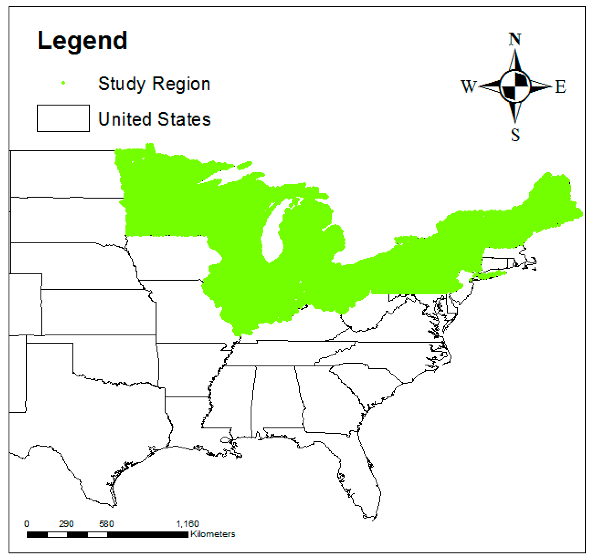
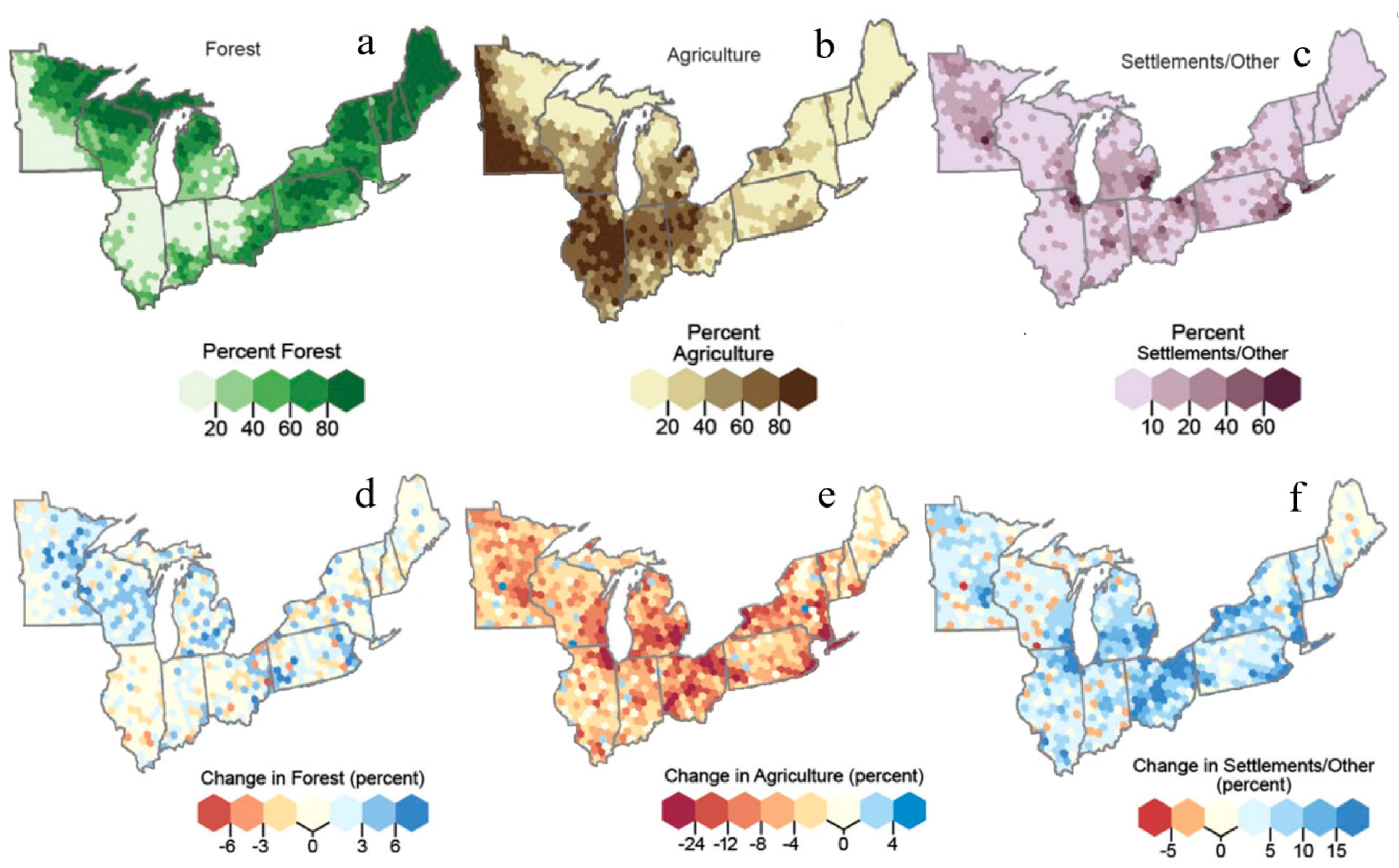
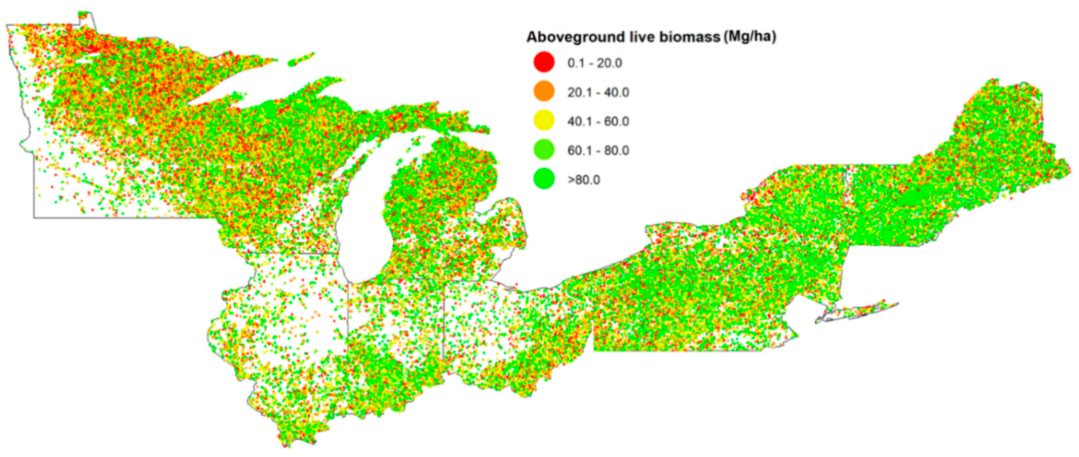
2.1. Research Region

The study domain covered eleven states in the Northern US including Minnesota, Wisconsin, Illinois, Indiana, Michigan, Ohio, Pennsylvania, New York, Vermont, New Hampshire, and Maine (Figure 1). The major land-cover types included forest (F), agriculture (A), and settlements/other (S, Figure 2). Forests were the dominant land use across nearly half (50.86%) of the Northern US. Forest land use was greatest (82.65%) in the upper Great Lakes and New England. Agriculture land use was most dominant in the Great Plains extending into Illinois, Indiana, and Ohio. Settlements/other was the dominant land use (17.28%) across portions of Ohio and New York (Figure 2). Across the Northern US, forestland areas of deforestation for F→A, F→S, and F→A&S decreased 331,711 ha, 408,482 ha, and 740,193 ha, respectively, during the remeasurement period of five years (one measurement during 2008–2012 and remeasured five years later during 2013–2018). Meanwhile, forestland areas of reforestation/afforestation for A→F, S→F, and A&S→F increased 946,968 ha, 323,456 ha, and 1,270,424 ha, respectively, during the five years (

Table 1. Land area changes (ha) from forest (F) to agriculture (A) and settlements/other (S), from agriculture and settlements/other to forest across the Northern US every five years.

Forest Area (ha)	F→A	F→S	F→A&S	A→F	S→F	A&S→F	F→A&S + A&S→F (Medium)
	331,711	408,482	740,193	946,968	323,456	1,270,424	530,231

and Figure 2). Forestland areas under medium LUC (F→A&S + A&S→F) increased 530,231 ha across the study area. This study region was ideal for examining LUC and disturbance impacts on forest AGB given the abundant forest cover in these areas and the wide range of land use and disturbance types affecting these systems.

2.2. National Forest Inventory Data

Comprehensive NFI data were extracted from the US Department of Agriculture Forest Service, Forest Inventory and Analysis (FIA) database (https://apps.fs.usda.gov/fia/datamart/datamart.html) in 11 states of the Northern US for a total of 78,458 plots (Figure 3, with one measurement between 2008 and 2012 remeasured five years later between 2013 and 2018). Each permanent ground plot was composed of four smaller fixed-radius (7.32 m) subplots spaced 36.6 m apart in a triangular arrangement around a central subplot. For each permanent ground plot, plot-level estimates of forest AGB (Figure 3), trees per hectare, basal area per hectare, and measurements of slope and elevation were used (

Table 2. Definitions and units of variables used in the study for matrix growth models.

Variables	Units	Definitions/Explanations
		Forest Inventory Data
AGB	Mg ha−1	Aboveground biomass
B	m2 ha−1	Total stand basal area
N	trees ha−1	Number of trees per hectare
S E	km	Plot slope Elevation
		Landsat Data
TCB	W m−2	Tasseled cap brightness
DI	W m−2	Disturbance index
EVI	unitless	Enhanced vegetation index
SWIR	nm	Shortwave infrared surface reflectance
TCG	W m−2	Tasseled cap greenness
SAVI	unitless	Soil adjusted vegetation index
TCA	W m−2	Tasseled cap angle

). Land use was characterized by a hexagonal grid from Woodall et al. [5] to facilitate analysis at spatial scales optimized for plot sampling intensity of the NFI. Land use change was estimated for each hexagon that had at least eight sample plots within it, with change calculated as the difference in the percent land use between time one and two by land use category. Detailed information about land use characterizations can be found in Woodall et al. [5].

2.3. Landsat Data

Landsat time-series data were obtained from the Google Earth Engine (https://earthexplorer.usgs.gov/). Landsat time-series data were acquired by Landsat 8 Operational Land Imager (OLI)/Thermal Infrared Sensor (TIRS), Landsat 7 Enhanced Thematic Mapper Plus (ETM+), Landsat 5 Thematic Mapper (TM), and Landsat 5 Multispectral Scanner (MSS) instruments from 2008 to 2018. Landsat 7 ETM+ and Landsat 8 OLI/TIRS data were processed upon download but used predicted ephemeris, initial bumper mode parameters, or initial TIRS line-of-sight model parameters. The data were reprocessed with definitive ephemeris, updated bumper mode parameters and refined TIRS parameters, and the products were transitioned to either Tier 1 or Tier 2 and removed from the Real-Time tier (https://landsat.usgs.gov/landsat-collections).

2.4. Description of the Matrix Models

Matrix growth models were applied to project AGB dynamics of remaining forests controlling for diameter growth, mortality, and recruitment as follows [35,36]:

$${\mathbf{y}}_{t+1}=G_t\cdot {\mathbf{y}}_t+R_t+\mathsf{\epsilon }$$

(1)

in which y_t and y_t+1 are number of live trees per hectare at time t and t + 1, respectively; G_t is a transition matrix describing how trees grow or die between t and t + 1; R_t is a recruitment vector representing the trees naturally recruited in the smallest diameter class between t and t + 1; ε is a random error; and G_t and G_it are state- and time-dependent transition matrices. G_it is a submatrix of G_t, where

$$\begin{gathered} G_t=\left[\begin{array}{cccc}{G}_1{}_t& & & \\ & G_2{}_t& & \\ & & \ddots & \\ & & & G_{i,t}\end{array}\right] \\ {G}_i{}_t=\left[\begin{array}{ccccc}{a}_{i1,t}& & & & \\ b_{i1,t}& a_{i2,t}& & & \\ & \ddots & \ddots & & \\ & & b_{i,j-2,t}& a_{i,j-1,t}& \\ & & & b_{i,j-1,t}& a_{i,j,t}\end{array}\right] \end{gathered}$$

(2)

in which a_ijt represents the probability that a tree of species group i and diameter class j stays alive in the same size class between t and t + 1. The transition probability of growth, b_ijt, represents a tree of species i, and diameter class j stays alive and grows into diameter class j + 1 between t and t + 1, assuming that trees were evenly distributed within a diameter class. b_ijt was estimated as the annual tree diameter growth, g_ijt, divided by the width of the diameter class. a_ijt and b_ijt are related by

$$a_{ijt}=1-b_{ijt}-m_{ijt}$$

(3)

where m_ijt is the tree mortality of species i and size class j between t and t + 1.

R_t represents the number of trees naturally recruited into the smallest size class of each species group, between t and t + 1. R_it is a sub vector of R_t representing recruitment of species group i at time t, where

$$R_t=\left[\begin{array}{c}{R}_{1t}\\ R_{2t}\\ ⋮\\ R_{m,t}\end{array}\right]R_i{}_t=\left[\begin{array}{c}{R}_{it}\\ 0\\ ⋮\\ 0\end{array}\right]$$

(4)

The annual diameter growth of the tree of species group i and size class j from t and t + 1 is represented by the following model ([27]; all notations defined in Table 2):

$$g_{ijt}={\alpha }_{i1}+{\alpha }_{i2}TCB+{\alpha }_{i3}DI+{\alpha }_{i4}EVI+{\alpha }_{i5}SWIR+{\alpha }_{i6}TCG+{\alpha }_{i7}SAVI+{\alpha }_{i8}TCA+{\alpha }_{i9}E+{\alpha }_{i10}S+{\theta }_{ij}$$

(5)

in which α_i’s are parameters to be estimated with the generalized least squares (GLSs, [37]) for diameter growth of species group i and size class j. $\theta$ is an error term.

Tree mortality of species group i and diameter class j at time t, m_ijt = P(M_ijt = 1|x) is estimated with a Probit function [38]. M_ijtk is a binary variable representing whether a tree of species i and diameter class j died (M_ijtk = 1) or not (M_ijtk = 0):

$$m_{ijt}=\Phi \left({\delta }_{i1}+{\delta }_{i2}TCB+{\delta }_{i3}DI+{\delta }_{i4}EVI+{\delta }_{i5}SWIR+{\delta }_{i6}TCG+{\delta }_{i7}SAVI+{\delta }_{i8}TCA+{\delta }_{i9}E+{\delta }_{i10}S+{\xi }_{ij}\right)$$

(6)

where Φ is the standard normal cumulative function, δ_i’s are parameters estimated by maximum likelihood, and $\xi$ is an error term.

For the recruitment of species group i, R_i is estimated with a Tobit model [39]:

$$R_{it}=\mathsf{\Phi }({\beta }_i{x}_{it}{\sigma }_i{}^{-1}){\beta }_i{x}_{it}+{\sigma }_i\varphi ({\beta }_i{x}_i{}_t{\sigma }_i{}^{-1})$$

(7)

with

$${\beta }_i{x}_{it}={\beta }_{i1}+{\beta }_{i2}TCB+{\beta }_{i3}DI+{\beta }_{i4}EVI+{\beta }_{i5}SWIR+{\beta }_{i6}TCG+{\beta }_{i7}SAVI+{\beta }_{i8}TCA+{\beta }_{i9}E+{\beta }_{i10}S+{\mu }_{ij}$$

(8)

where Φ is the standard normal cumulative distribution function, φ is the standard normal probability density function, and $\mu$ is an error term. The Tobit model explicitly accounts for unobserved recruitment values that are left-censored at the preset diameter limit.

The forest AGB C density is estimated with the following model [27]:

$${\psi }_{it}={\omega }_{i1}+{\omega }_{i2}TCB+{\omega }_{i3}DI+{\omega }_{i4}EVI+{\omega }_{i5}SWIR+{\omega }_{i6}TCG+{\omega }_{i7}SAVI+{\omega }_{i8}TCA+{\omega }_{i9}E+{\omega }_{i10}S+{\omega }_i$$

(9)

in which ${\psi }_i$ is a vector of forest AGB C density, ${\omega }_i$’s are parameters to be estimated with the GLS, $\omega$ is an error term, and ${\psi }_i$ is calculated with Equation (9).

For the future simulations using matrix growth models, a certain percentage of trees were removed under disturbances and added under LUC (F→A&S + A&S→F) every five years. In order to backcast forest AGB dynamics using matrix growth models from 2018 to 1998, we applied similar annual rates of mortality and recruitment, minus the annual rate of tree growth, without considering LUC and disturbances. Stand density was set to zero if stand age was less than 20 years.

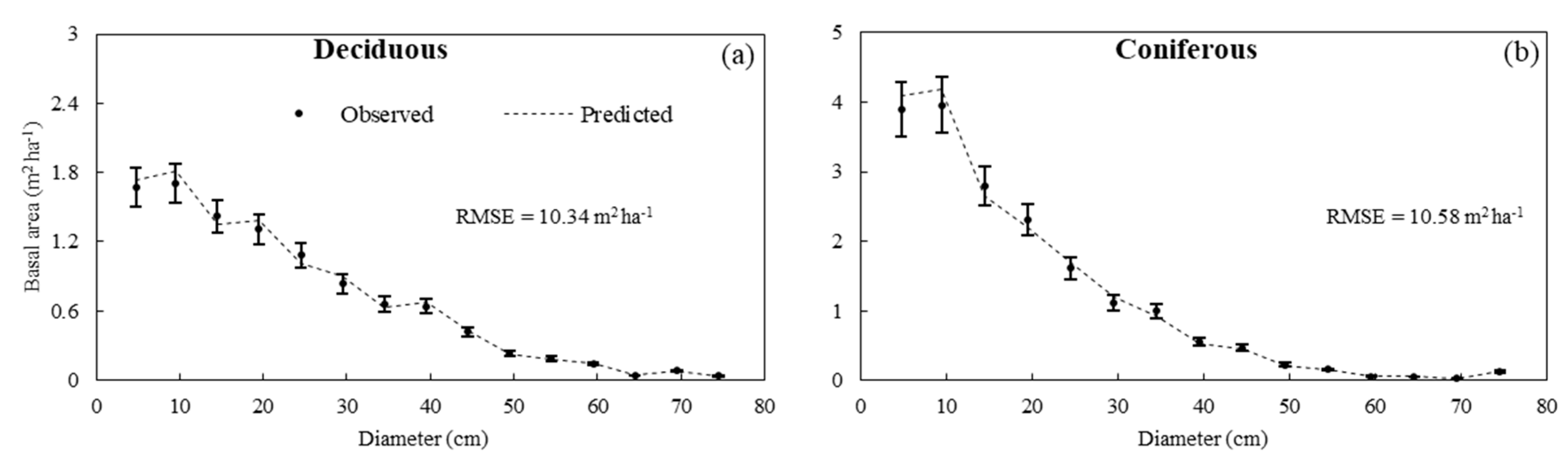
2.5. Model Calibration and Validation

We adopted the same variables and functional form for the underlying diameter growth, mortality, recruitment, and AGB models as those established in previously published matrix models [27] to maintain accuracy and avoid overfitting and multicollinearity between predicted variables. A variety of stand level and Landsat variables selected for two species groups (deciduous and coniferous) were used in the matrix growth models (

Table 3. Estimated parameters of the diameter growth model, mortality model, recruitment model, and aboveground biomass model in the matrix growth models.

Diameter Growth Model

Deciduous

0.521** − 0.176TCB* − 0.535DI* + 0.458EVI** + 0.233SWIR* − 0.818TCG** + 0.925SAVI* + 0.346TCA − 0.825E* − 0.668S* (R2 = 0.62)

Coniferous

0.668** − 0.186TCB** − 0.719DI** + 0.389EVI* + 0.847SWIR − 0.279TCG* + 0.774SAVI** + 0.638TCA* − 0.796E** − 0.369S* (R2 = 0.59)

Mortality Model

Deciduous

0.822* + 0.678TCB* − 0.846DI** − 0.868EVI** + 0.186SWIR* + 0.046TCG* + 0.798SAVI* − 0.337TCA* − 0.857E* − 0.668S** (R2 = 0.38)

Coniferous

0.935* + 0.547TCB** − 0.869DI* − 0.845EVI** + 0.578SWIR* + 0.844TCG* + 0.362SAVI* − 0.878TCA* − 0.814E* − 0.667S (R2 = 0.35)

Recruitment Model

Deciduous

0.667** − 0.879TCB* − 0.845DI** + 0.868EVI** + 0.887SWIR** + 0.935TCG* − 0.148SAVI* + 0.892TCA** − 0.146E − 0.756S* (R2 = 0.23)

Coniferous

0.764** − 0.164TCB** − 0.396DI** + 0.446EVI** + 0.868SWIR* + 0.516TCG* − 0.593SAVI* + 0.827TCA − 0.357E** − 0.784S* (R2 = 0.21)

Aboveground Biomass Model

0.368*** − 0.636TCB** − 0.768DI* + 0.234EVI** + 0.372SWIR* + 0.885TCG** + 0.936SAVI* + 0.185TCA* − 0.355E* − 0.885S** (R2 = 0.73)

Significance levels: * < 0.05; ** < 0.01; *** < 0.001.

). Physiographic variables, elevation (E) and slope (S), were used to control for site productivity [40]. Landsat variables, tasseled cap brightness (TCB), disturbance index (DI), enhanced vegetation index (EVI), shortwave infrared surface reflectance (SWIR), tasseled cap greenness (TCG), soil adjusted vegetation index (SAVI), and tasseled cap angle (TCA) were used to replace total stand basal area (B) as key predictors, due to the correlation between the Landsat predictors and forest stand characteristics [27]. For model calibration purposes, 62,766 permanent ground plots (80%) and plot-corresponded Landsat data were used to estimate parameters of the matrix growth model. In addition, model validation (the rest: 15,692 permanent ground plots, 20%) followed Ma et al. [27], where matrix models were used to enable various combinations of LiDAR, Landsat, and field data, especially Landsat data to estimate large-scale AGB dynamics (i.e., the central component of carbon stock monitoring) without loss of accuracy from only using variables from forest inventories (Figure 4). Finally, the 15,692 permanent ground plots and plot-corresponded Landsat data were applied to make the future predictions.

2.6. Land Use Change and Disturbance Scenarios

Recent studies have suggested that LUC and forest disturbances (e.g., harvest, wildfire, insects and diseases, and weather) simultaneously affect regional forest C uptake [2,5,6,24]. Thus we used three general land use categories following Woodall et al. [5]: forest (F), agriculture (A), and settlements (S, urbanization/other). In addition, we explored effects of disturbances such as harvest, wildfire, insects and diseases, and weather with low, medium, and high severity/intensity (

Table 4. Average annual disturbance rates with low (L), medium (M), and high (H) severity in the study region.

Forest Area (%)	Harvest	Fire	Insect and Disease	Weather
Low	6.0	0.5	3.4	2.3
Medium	7.0	1.5	4.4	3.3
High	8.0	2.5	5.4	4.3

). Annual medium disturbance rates (percent of the forest area influenced per year) were obtained and bounded from Wear and Coulston [6] for the Northern US based on empirical information. Moreover, average annual LUC and disturbance rates increased by 1% from low-to-medium to medium-to-high severity for sensitivity analysis. Based on the average annual disturbance rates, we assumed 50% removal (i.e., mortality and subsequent C emission) of all trees subject to fire, insects and diseases, and weather, and only removal of large trees (greater than 40 cm) under harvesting. In order to study the effects of LUC, disturbances, and their comprehensive effects on forest C dynamics, we predicted future total forest AGB dynamics considering scenarios of LUC and disturbances every five years (same period with historical LUC) from 2018 to 2098. The scenarios were defined as follows: (a) LUC included F→A, F→S, F→A&S, A→F, S→F, A&S→F, and F→A&S + A&S→F with low, medium, and high intensity; (b) Disturbances included fire, weather, insect and disease, and harvest with low, medium, and high severity; (c) Medium LUC + disturbances included LUC + fire, LUC + weather, LUC + insect and disease, and LUC + harvest.

Effects of LUC and disturbances were added in the forest AGB dynamics every five years from 2018 to 2098. Forest AGB C changes induced from LUC and disturbances were estimated as follows: forest AGB C changes from LUC and disturbances = forestland area changes from LUC and disturbances × forest AGB C density.

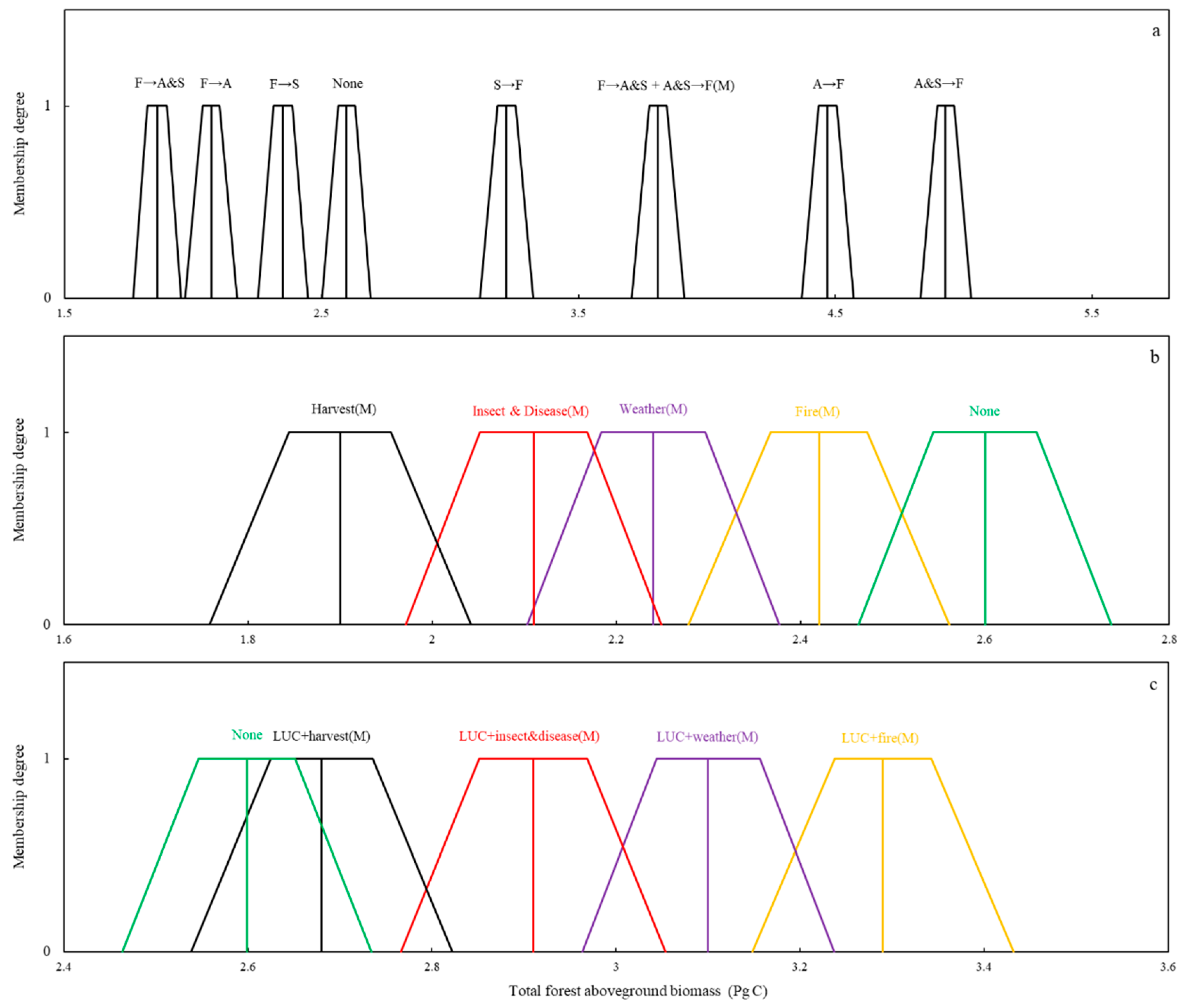
2.7. Fuzzy Sets representing LUC and Disturbance Uncertainty

Uncertainty analysis is a necessary procedure in model simulation [16]. Uncertain LUC and disturbances in future have led to high variability in predicted values of forest AGB. The averages of predicted forest AGB are important point estimates, but understanding the associated risk, ranges, or sets indicating prediction uncertainty is essential. To more accurately quantify this uncertainty, we used fuzzy sets, which involved defining membership functions that determined the level of uncertainty [41]. The theory of fuzzy promulgates the concept of a possibility distribution as a fuzzy restriction acting as a flexible constraint on the average values that may be assigned to a variable [41]. A trapezoidal fuzzy set was used, mathematically expressed as f (x; a, b, c, d) = max (min (x − ab − a, 1, d − xd − c), 0). [a,b] and [c,d] are the uncertainty intervals with membership degrees ranging from 0 to 1. [b,c] represents the certainty interval for which the membership degree is 1. [a,d] is a measure of the total range of uncertainty arising from LUC and disturbance occurrences. Given the average value of predicted forest AGB ($\overline{X}$) and its relative standard deviation (S_r) from simulations, a, b, c, and d values can be calculated as follows [42]:

$$\begin{gathered} \mathrm{b}=\frac{\overline{X}}{1+0.5{\mathrm{S}}_r} \\ \mathrm{c}=\overline{X}(1+0.5{\mathrm{S}}_{\mathrm{r}}) \\ \mathrm{a}=\mathrm{b}-\overline{X}(\frac{1}{1+0.5{\mathrm{S}}_r}-\frac{1}{1+2.5{\mathrm{S}}_r}) \\ \mathrm{d}=\mathrm{c}+\overline{X}·2{\mathrm{S}}_{\mathrm{r}} \end{gathered}$$

(10)

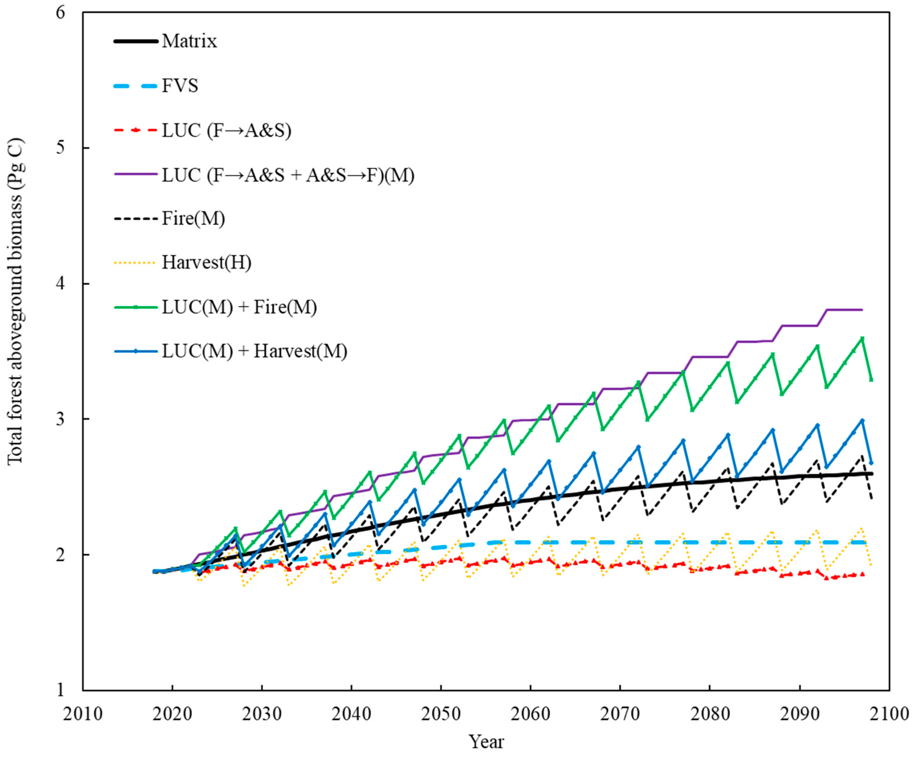
2.8. Forest Vegetation Simulator Comparisons

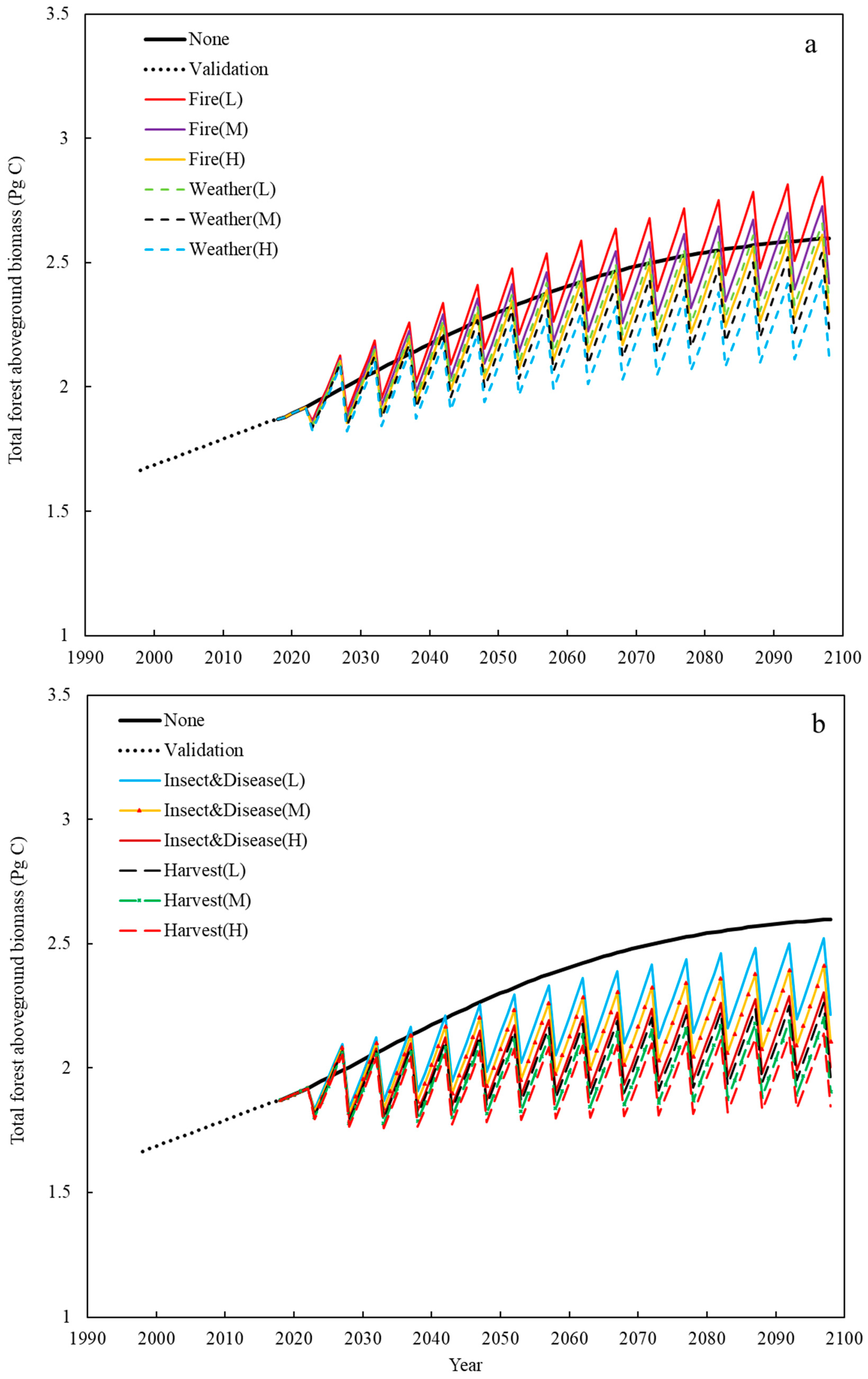
In order to more thoroughly evaluate our matrix model predictions of AGB accumulation, forest inventory plot attributes (e.g., tree abundance by species and diameter class, and AGB) were projected using a forest stand vegetation simulator (FVS). Similar to the matrix growth models, FVS is a simulation tool that relies on empirical growth and yield models that have been extensively used in the US [43]. FVS is used broadly to predict forest stand dynamics, and is an approved quantification tool by the American C Registry [44]. Stand condition by the year 2018, which was the same as the matrix models, was executed as the starting point. The TREEBIO report from the FVS was used to provide plot-level AGB outputs for the same research area. Then, area-wide total forest AGB was projected for the future 80 years at decadal intervals until 2098, without considering LUC and disturbances.

3. Results

Based on the 80-year future predictions (2018–2098), total forest AGB of the Northern US would increase over time from 2018 (1.88 Pg C) and converge to ~2.60 Pg C by 2098 without considering LUC and disturbances (scenario none, Figure 5). Total forest AGB would increase 38.30% under the condition of natural growth over the next 80 years. Comparing matrix model predictions of AGB with FVS predictions, our models predicted higher forest AGB over time, with a 24.13% increase in forest AGB by the end of period. In addition, we also made backward validation of total forest AGB from 2018 to 1998 without considering LUC and disturbances (Figure 5). Forest AGB increased from 1.67 to 1.88 Pg C, with an increase of 12.57% during 20 years from 1998 to 2018.

Considering only disturbances of low, medium, and high severity, total forest AGB subject to all disturbance types would decrease by the year 2098 compared with natural growth without considering LUC and disturbances (scenario none) (

Table 5. Predicted total forest aboveground biomass (Pg C) from 2018 to 2098 under disturbances (harvest, fire, insect and disease, and weather) with low, medium, and high severity in the Northern US. I&D: insects and disease.

	2018	2028	2038	2048	2058	2068	2078	2088	2098
	Low
Harvest	1.88	1.79	1.81	1.85	1.88	1.90	1.92	1.94	1.96
Fire	1.88	1.90	2.02	2.15	2.26	2.35	2.42	2.48	2.53
I&D	1.88	1.84	1.91	1.99	2.05	2.10	2.14	2.18	2.21
Weather	1.88	1.86	1.95	2.06	2.14	2.20	2.26	2.30	2.35
					Medium
Harvest	1.88	1.78	1.79	1.82	1.84	1.85	1.87	1.88	1.90
Fire	1.88	1.88	1.98	2.09	2.18	2.26	2.32	2.37	2.42
I&D	1.88	1.82	1.87	1.93	1.98	2.01	2.05	2.08	2.11
Weather	1.88	1.84	1.91	2.00	2.06	2.12	2.16	2.20	2.24
	High
Harvest	1.88	1.76	1.76	1.78	1.80	1.81	1.82	1.83	1.85
Fire	1.88	1.86	1.94	2.03	2.11	2.17	2.22	2.26	2.30
I&D	1.88	1.80	1.83	1.87	1.91	1.93	1.96	1.98	2.00
Weather	1.88	1.82	1.87	1.94	1.99	2.03	2.07	2.10	2.13

and Figure 5). With medium severity, total forest AGB due to fire, weather, insect and disease, and harvest would become 2.42, 2.24, 2.11, and 1.90 Pg C, respectively, at the end of period. From low-to-medium and medium-to-high severity (1% annual disturbance rate increase), the total forest AGB subject to fire would decrease by 0.11 and 0.12 Pg C by the year 2098, respectively. In addition, forest AGB subject to fire, weather, insect and disease, and harvest with high severity would decrease by 11.54%, 18.08%, 23.08%, and 28.85%, respectively, from 2018 to 2098, in comparison with a scenario without any affecting factors (referred to hereafter as “scenario none”) (Figure 5).

When only considering LUC, predicted total forest AGB subject to conversions of F→A, F→S, A→F, S→F, A&S→F, and medium F→A&S + A&S→F is projected to increase over time from 2018 to 2098 (Figure 6a), while F→A&S would result in a decrease in forest AGB. The forest AGB subject to conversions of F→A&S, A&S→F, and medium F→A&S + A&S→F would be 1.86, 4.93, and 3.81 Pg C, respectively, by the year 2098 (Figure 6a). Deforestation including F→A and F→S would have forest AGB increases of 10.11% and 25.00%, respectively, while F→A&S would decrease 1.06% by the year 2098 compared to the year 2018. Reforestation and afforestation including conversions of A→F, S→F, and A&S→F would increase forest AGB by 137.77%, 71.28%, and 162.23%, respectively, by the end of simulations. LUC (F→A&S + A&S→F) with low, medium, and high intensity (i.e., 1% increase of annual LUC rates from low-to-medium and medium-to-high) would result in 79.52%, 102.66%, 119.26% increases in total forest AGB, respectively, over the next 80 years (Figure 7). Additionally, predicted forest AGB subject to conversions of F→A, F→S, and F→A&S were less than scenario none (i.e., no land use change or disturbances) while A→F, S→F, A&S→F, and all intensities of F→A&S + A&S→F were greater than scenario none (Figure 6a and Figure 7).

When simultaneously considering both LUC and disturbances in medium severity, total forest AGB predictions of LUC + fire, LUC + weather, LUC + insect and disease, and LUC + harvest increased over time from 2018 to 2098 (Figure 6b and Figure 7). Total forest AGB of LUC + fire, LUC + weather, LUC + insect and disease, and LUC + harvest would reach to 3.29, 3.10, 2.91, and 2.68 Pg C, respectively, by the year 2098. With medium severity, LUC + fire (annual rate 1.5%) and LUC + harvest (annual rate 7%) would increase 75.00% and 42.55% of forest AGB over the next 80 years (Figure 6). Aboveground biomass on forestland subject to LUC + harvest and LUC + insect and disease would reduce AGB by 18.54% and 11.55% relative to AGB accumulation subject to LUC + fire by the year 2098. LUC + fire had the smallest increase, while the LUC + harvest had the largest increase for all predictions over the next 80 years.

To account for variability induced by medium LUC and disturbances, fuzzy sets were constructed for predicting forest AGB in the year 2098 (Figure 8). Considering only LUC, A&S→F clearly outperformed the other scenarios by storing the highest total forest AGB with high certainty. Considering only disturbances, fire would lead to the highest total forest AGB under all disturbance scenarios. Weather and insect and disease would have a similar total forest AGB in the year 2098. When considering both medium LUC and disturbances, most LUC + disturbances would in general lead to higher forest AGB than undisturbed forest growth with high certainty.

4. Discussion

4.1. Matrix Growth Models for Predicting Forest AGB Dynamics from 2018 to 2098

Matrix growth models are useful for predicting forest population dynamics and associated forest C dynamics under varying natural disturbances, management, and climate scenarios through consideration of diameter growth, mortality, and recruitment [15,16,26,27,35,36,45]. Moreover, matrix growth models are highly accurate in characterizing forest C dynamics over large-scale forest areas based on empirical forest inventories and Landsat data [27]. Applying selected Landsat variables, we revalidated the strength of Landsat dependent matrix growth models in their applications for predicting large-scale forest AGB dynamics [27]. Such an assertion is supported by Ma et al. [27], who suggested that Landsat variables can be used to replace stand basal areas to predict AGB at landscape scales. Moreover, we found that predicted forest AGB increased over time and converged to ~2.60 Pg C by 2098 through natural accretion of biomass (i.e., absent of disturbance and LUC). This finding is supported by prior studies which suggested that total forest AGB accumulation should increase towards a theoretical maximum within a certain period of time [26,27,45,46,47,48,49]. Over the next 80 years, we found that total forest AGB would increase 38.30% across the study area without considering LUC and disturbances. This is consistent with other studies that have estimated potential regional forest AGB C stock increases of 15%–50% over the next 50–100 years [46,50,51]. Besides the standard FVS outputs (stem density, basal area, volume, etc.), tailored C output provided estimates of total forest AGB of the Northern US from 2018 to 2098. In comparison with the FVS, the matrix growth models projected greater total forest AGB over time and predicted more total forest AGB (24.13%) by the year 2098. The possible explanation is that FVS projects recruitment and regeneration if (and only if) the stand density is below a predesignated threshold value [30,52], and such underestimation of recruitment in FVS predictions would systematically affect the accuracy of the entire model. As a substantial portion of tree regeneration in the study region is derived from natural regeneration [53], restrictions on tree recruitment during modeling exercises such as the FVS might reduce future estimates of tree stocking and hence AGB accumulation.

4.2. Backward Validation of Matrix Models from 2018 to 1998

As signatories to the United Nations Framework Convention on Climate Change (UNFCCC), the US has reported economy-wide greenhouse gas emissions and removals each year from 1990 to the near present [4]. In addition, the Intergovernmental Panel on Climate Change (IPCC) requires that emissions and removals associated with changes in land use be attributed to specific activities. In order to harmonize IPCC reporting requirements with scenario testing for determining national future commitments, we made backward validations of forest AGB from 2018 to 1998 and found that forest AGB increased from 1.66 to 1.88 Pg (13.25%) during this time period across the Northern US. This provides a baseline for reporting C emissions and removals from 1990 to the present. Moreover, such backward validations of large-area AGB could be further applied to provide spatially explicit contemporary baseline assessments as a means of refining US greenhouse gas (GHG) estimates.

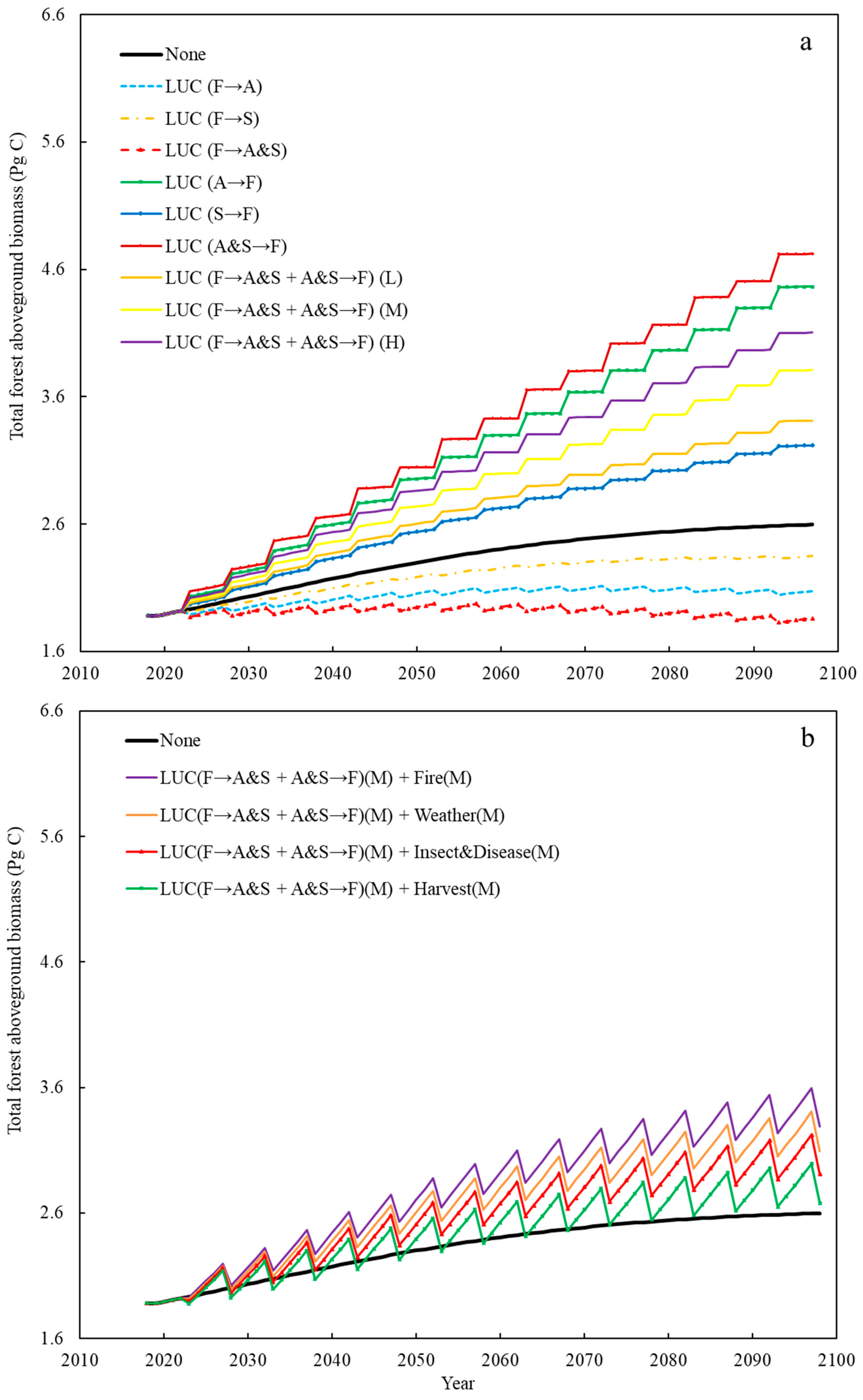
4.3. Effects of LUC, Disturbances, and Their Interactions on Future Forest AGB Dynamics

Land use change may substantially influence future C dynamics over time [54,55]. Quantifying forest C dynamics associated with LUC is important for forest C monitoring and UNFCCC reporting [5]. Conversions from agriculture and settlements/other to forestland have been occurring, which substantially offsets net C emissions across the globe. In addition, post potential forest AGB C uptake induced by decreased forest land area could be offset by increases in forest AGB via elevated forest growth [6]. Medium LUC increased total forest AGB by 1.21 Pg C over the next 80 years. This finding is consistent with prior studies that have strongly suggested LUC as a major driver of the forest C sink in the US [5,10,11,56]. Nevertheless, Birdsey et al. [57] estimated that the settlement and subsequent deforestation and/or intensive harvest of US forests emitted over 4.0 Pg C between 1715 and 1935. Most of those C emissions would not be compensated by future northern forest C accumulation via LUC and natural forest growth. The strong C uptake estimated in privately owned forestland implies that positive land use planning and forest management might be one opportunity to maintain C sink strength [5,53]. Although maintaining forestland via conservation measures will be one policy consideration in the future, additional approaches such as reforestation and afforestation concomitant with tightly coupled forest management and long-lived forest product industries might be needed to ensure maximum terrestrial C accumulation within diverse land uses in a context of global change (i.e., invasive, browse, CO₂ enrichment).

Natural and human disturbances such as wildfire, insect and disease outbreaks, weather, and timber harvesting could cause forest C uptake losses that potentially alter the directionality of C fluxes in forests [19,58,59]. Disturbance events may decrease forest AGB accumulation if annual disturbance rates increase every 1% across the Northern US (Table 4 and Table 5). Except for growth enhancements, forest C stocks accrete mainly due to the net effect of disturbances and regrowth. Forest C stock accumulation under disturbances would be less than C stored from natural growth if disturbances led to additional C stock losses than the resulting offset of forest recovery and growth enhancements (e.g., density reduction of overstocked stands). Another possible explanation for such a decrease is that higher severity of natural disturbances could increase tree mortality and suppress tree growth in stands, which in turn may reduce forest AGB growth [16,60,61]. Moreover, some of the predicted C stock losses may be captured in harvested wood products (0.58 Pg C). Although natural disturbances may initiate a regeneration legacy that contributes considerably to the increased rate of forest C stocks [58], it might be more than offset by C sequestration potential losses induced by greater mortality compared with forest natural growth. However, disturbance scenarios with low/medium fire and low weather may lead into higher total forest AGB than no disturbances during some periods in the future simulations due to the low and/or mixed severity nature of such disturbances, which can create mortality in the suppressed cohorts of many stands. Such mortality can lead to increased growth of survivors in combination with the regeneration of new, potentially rapidly growing cohorts [62]. The sensitivity analysis of disturbances suggested that disturbances with higher severity would lead to less forest AGB sequestration potential across the study region. This is consistent with other studies that imply that the majority of forest C stocks decrease with greater harvest levels and increased disturbance rates [58,63]. Maintaining or increasing forest C stocks will be very challenging if disturbance percentages increase substantially over the next several decades [63,64]. Moreover, disturbances would not be the only process influencing forest AGB dynamics, as other global change factors, including increased atmospheric CO₂ and N deposition, may also be other factors to consider. Without accounting explicitly for these factors in this study, we propose that tremendous uncertainty surrounds the true risk of reductions in C sequestration rates. Additionally, although changes in the frequency and severity of disturbances are forecast to occur under global climate change, we did not study the influences of climate change and interactions between disturbance events and a warmer climate. In all, our study has addressed the effects of most types of disturbances on future forest AGB dynamics in the Northern US.

Although LUC and disturbances have collectively affected terrestrial C dynamics over time, few studies have attempted to characterize the interactive impact of simultaneous changes in LUC and disturbance processes on future forest AGB dynamics [7,20,22,34,54,65]. Our findings indicate that contemporary LUC substantially contributes to forest C sink, and forest C sequestration rates may increase as well under interactions of LUC and disturbances in Northern US forests. Combined medium LUC and disturbances could keep the region’s forests as a C sink, which suggests that positive effects of medium LUC would not be offset by negative influences of medium disturbances. Under a 7.0% annual harvest rate (including partial cutting of large trees), we estimate a decrease of 4.26% of total forest AGB in the LUC + harvest scenario compared with a natural growth (scenario none). This is consistent with other studies that have focused on the potential for active LUC planning and altered forest management practices, which has been viewed as a potential opportunity to maintain regional C sink strength [5,63].

4.4. Uncertainty Estimation

Taking into consideration uncertainty arising from LUC and disturbances is useful and important in large-scale predictions of forest C dynamics [66] and is a requirement in UNFCCC reporting [26]. Long-term forest C simulations were subject to the bias caused by the changes in LUC (i.e., from non-forest to forest or from forest to non-forest). Disturbances could affect C sequestration, as C could rapidly move from living biomass to dead organic matter or to the atmosphere via combustion [67]. In this study, we only focused on parameter uncertainty in LUC and disturbances, which mostly stems from measurement errors, missing data, or unrepresentative data [68]. We used fuzzy sets to estimate the parameter uncertainty in terms of membership degree, as fuzzy set theory can provide a useful point of departure for the construction of a conceptual framework, which may prove to have a much wider scope of applicability [41]. To handle uncertainty of parameters in the forest AGB predictions, a two-step approach can be adopted. First, Monte Carlo simulations [69] could be used to produce random realizations of possible parameters, thus generating the average and relative standard deviations of outputs. Then, uncertainty in forest AGB predictions of LUC and disturbance scenarios with fuzzy sets could determine the level of output uncertainty caused by uncertain parameter inputs. The uncertainty range of outcomes related to LUC and disturbance scenarios showed LUC and disturbances to be perhaps the most important uncertainty regarding the strength of the forest C sink. Nevertheless, hindered by the complexity of modeling fundamental disturbance processes in forests, we only applied annual disturbance rates to explore impacts of disturbances on forest AGB dynamics every five years. More importantly, we only examined the possible ranges in forest AGB predictions as an index of uncertainty while not explicitly examining detailed regimes of harvest, weather, wildfire, insect and disease, or other disturbance regimes. Admittedly, this study only dealt with very limited sources of uncertainty. Exploring more detailed and deeper sources of uncertainty is appropriate to estimate the uncertainty associated with forest AGB dynamic predictions. As such, caution should be extended to applying this study’s models in the context of individual drivers of C flux.

4.5. How Might We Increase the Forest AGB C Sink in the Northern US?

Modeling forest AGB C dynamics under LUC and disturbances is needed to help design policies increase forest C uptake in the US. In order to enhance regional AGB C sinks, development of long-term land use planning policy should explicitly recognize the importance of maintaining forestland use and maximizing reforestation/afforestation activities. Land use and forest dynamics should be simultaneously considered when projecting forest AGB C uptake across landscapes [5]. Forest AGB C operations should take into account warmer and more variable climates, as well as associated changes of disturbance severity and frequency [70]. Moreover, tremendous forest AGB C stocks still exist that need to be maintained, even as forest AGB C uptake may decrease in the future. Research efforts should focus on exploring and understanding the influence of changing disturbance regimes on post-disturbance forest conditions. Monitoring efforts should reach a clear identification of forest AGB C dynamics for different LUC and disturbance categories.

4.6. Future Work

Although we used matrix models combining plot-level physiographic variables (elevation and slope) with Landsat data to project future total forest AGB dynamics influenced by LUC and disturbance scenarios, we did not produce spatially explicit estimates regarding where risks and opportunities lie across the landscape for C accumulation. Additionally, we only considered forest AGB C gain/loss inducements from increases/decreases of forestland. In the future, we can directly obtain the physiographic variables from the digital elevation model (DEM) of the US Geological Survey (USGS). Dynamics of larger area AGB and other C pools (belowground biomass, soil C, dead wood C, and litter C) could be mapped using matrix models to allow for the inclusion of DEM and Landsat data to improve pixel-level prediction under LUC and disturbances. Transfers of C pools to and from each land use category could be considered as well. Such a development would allow forest C estimation to move from just being spatially explicit to spatially explicit and continuous while incorporating the temporal flexibility that comes with Landsat time series considering LUC.

5. Conclusions

There is a confluence of factors that may drive future trajectories of AGB C uptake in forests, especially when disturbances and LUC are considered. In the Northern US, when only considering LUC, total forest AGB of A&S→F and medium F→A&S + A&S→F would increase from 1.88 to 4.93 and 3.81 Pg C, respectively, by the end of the 21st century (year 2098). When only medium disturbances were considered, predicted forest AGB associated with forests subject to fire and harvest would increase from 1.88 to 2.42 and 1.90 Pg C, respectively, over the next 80 years. When both medium LUC and disturbances are considered, forest AGB predictions of LUC + fire, LUC + weather, LUC + insect and disease, and LUC + harvest would increase from 1.88 to 3.29, 3.10, 2.91, and 2.68 Pg C, respectively. At a medium level, an uncertainty analysis with fuzzy sets indicated that LUC + fire would lead to the highest forest AGB, and LUC + harvest would lead to the lowest forest AGB by the end of period. This study confirms that LUC is an important driver of the forest C sink in the Northern US, while disturbances may lend themselves toward C emissions compared with natural growth (scenario none), exclusive of impending global change threats such as invasives or CO₂ enrichment. Landsat data coupled with empirical field observations of forest C pools were used in this study, and the opportunity exists to more tightly link national C reporting requirements (i.e., 1990–baseline year reporting) with the need for spatially explicit estimates of future forest C dynamics as affected by LUC and disturbance scenarios. Finally, as several caveats (i.e., C emission rates per specific disturbance events) were applied in this study for the development of initial C trajectories (~80 years into the future), there are opportunities to explore alternative emission and removal factor estimates with emerging science.

References

1. Intergovernmental Panel on Climate Change (IPCC). Climate Change 2013: The Physical Science Basis. Working Group I Contribution to the IPCC 5th Assessment Report—Changes to the Underlying Scientific/Technical Assessment; Cambridge University Press: New York, NY, USA, 2013. [Google Scholar]
2. Law, B.E.; Hudiburg, T.W.; Berner, L.T.; Kent, J.J.; Buotte, P.C.; Harmon, M.E. Land use strategies to mitigate climate change in carbon dense temperate forests. Proc. Natl. Acad. Sci. USA 2018, 115, 3663–3668. [Google Scholar] [CrossRef] [PubMed] [Green Version]
3. Schurman, J.S.; Trotsiuk, V.; Bače, R.; Čada, V.; Fraver, S.; Janda, P.; Kulakowski, D.; Labusova, J.; Mikoláš, M.; Nagel, T.A.; et al. Large-scale disturbance legacies and the climate sensitivity of primary Picea abies forests. Glob. Chang. Biol. 2018, 24, 2169–2181. [Google Scholar] [CrossRef] [PubMed]
4. Domke, G.M.; Walters, B.F.; Nowak, D.J.; Smith, J.E.; Ogle, S.M.; Coulston, J.W. Greenhouse Gas Emissions and Removals from Forest Land and Urban Trees in the United States, 1990–2017; Resource Update FS-178; Department of Agriculture, Forest Service, Northern Research Station: Newtown Square, PA, USA, 2019; 4p. [Google Scholar]
5. Woodall, C.W.; Walters, B.F.; Coulston, J.W.; D’Amato, A.W.; Domke, G.M.; Russell, M.B.; Sowers, P.A. Monitoring network confirms land use change is a substantial component of the forest carbon sink in the eastern United States. Sci. Rep. 2015, 5, 17028. [Google Scholar] [CrossRef] [PubMed]
6. Wear, D.N.; Coulston, J.W. From sink to source regional variation in US forest carbon futures. Sci. Rep. 2015, 5, 16518. [Google Scholar]
7. Yu, Z.; Lu, C.; Cao, P.; Tian, H. Long-term terrestrial carbon dynamics in the Midwestern United States during 1850–2015: Roles of land use and cover change and agricultural management. Glob. Chang. Biol. 2018, 24, 2673–2690. [Google Scholar] [CrossRef] [PubMed]
8. Ramankutty, N.; Foley, J.A. Estimating historical changes in land cover: North American croplands from 1850 to 1992: GCTE/LUCC RESEARCH ARTICLE. Glob. Ecol. Biogeogr. 1999, 8, 381–396. [Google Scholar] [CrossRef]
9. Houghton, R.A.; House, J.I.; Pongratz, J.; Van Der Werf, G.R.; DeFries, R.S.; Hansen, M.C.; Quéré, C.L.; Ramankutty, N. Carbon emissions from land use and land-cover change. Biogeosciences 2012, 9, 5125–5142. [Google Scholar] [CrossRef] [Green Version]
10. Caspersen, J.P.; Pacala, S.W.; Jenkins, J.C.; Hurtt, G.C.; Moorcroft, P.R.; Birdsey, R.A. Contributions of land-use history to carbon accumulation in US forests. Science 2000, 290, 1148–1151. [Google Scholar] [CrossRef]
11. Albani, M.; Medvigy, D.; Hurtt, G.C.; Moorcroft, P.R. The contributions of land-use change, CO2 fertilization, and climate variability to the Eastern US carbon sink. Glob. Chang. Biol. 2006, 12, 2370–2390. [Google Scholar] [CrossRef]
12. Ollinger, S.V.; Aber, J.D.; Reich, P.B.; Freuder, R.J. Interactive effects of nitrogen deposition, tropospheric ozone, elevated CO2 and land use history on the carbon dynamics of northern hardwood forests. Glob. Chang. Biol. 2002, 8, 545–562. [Google Scholar] [CrossRef]
13. Houghton, R.A. Revised estimates of the annual net flux of carbon to the atmosphere from changes in land use and land management 1850–2000. Tellus B 2003, 55, 378–390. [Google Scholar]
14. Houghton, R.A. Aboveground forest biomass and the global carbon balance. Glob. Chang. Biol. 2005, 11, 945–958. [Google Scholar] [CrossRef]
15. Ma, W.; Liang, J.; Cumming, J.R.; Lee, E.; Welsh, A.B.; Watson, J.V.; Zhou, M. Fundamental shifts of central hardwood forests under climate change. Ecol. Model. 2016, 332, 28–41. [Google Scholar] [CrossRef] [Green Version]
16. Ma, W.; Zhou, M. Assessments of harvesting regimes in central hardwood forests under climate and fire uncertainty. For. Sci. 2017, 64, 57–73. [Google Scholar] [CrossRef]
17. Seidl, R.; Thom, D.; Kautz, M.; Martin-Benito, D.; Peltoniemi, M.; Vacchiano, G.; Wild, J.; Ascoli, D.; Petr, M.; Honkaniemi, J.; et al. Forest disturbances under climate change. Nat. Clim. Chang. 2017, 7, 395. [Google Scholar] [CrossRef] [PubMed]
18. Nabuurs, G.J.; Schelhaas, M.J.; Mohren, G.M.; Field, C.B. Temporal evolution of the European forest sector carbon sink from 1950 to 1999. Glob. Chang. Biol. 2003, 9, 152–160. [Google Scholar] [CrossRef]
19. Kurz, W.A.; Stinson, G.; Rampley, G.J.; Dymond, C.C.; Neilson, E.T. Risk of natural disturbances makes future contribution of Canada’s forests to the global carbon cycle highly uncertain. Proc. Natl. Acad. Sci. USA 2008, 105, 1551–1555. [Google Scholar] [CrossRef]
20. Breshears, D.D.; Allen, C.D. The importance of rapid, disturbance-induced losses in carbon management and sequestration. Glob. Ecol. Biogeogr. 2002, 11, 1–5. [Google Scholar] [CrossRef]
21. Easterling, D.R.; Meehl, G.A.; Parmesan, C.; Changnon, S.A.; Karl, T.R.; Mearns, L.O. Climate extremes: Observations, modeling, and impacts. Science 2000, 289, 2068–2074. [Google Scholar] [CrossRef]
22. Smith, T.M.; Shugart, H.H. The transient response of terrestrial carbon storage to a perturbed climate. Nature 1993, 361, 523. [Google Scholar] [CrossRef]
23. Kirilenko, A.P.; Solomon, A.M. Modeling dynamic vegetation response to rapid climate change using bioclimatic classification. Clim. Chang. 1998, 38, 15–49. [Google Scholar] [CrossRef]
24. Alexander, P.; Rabin, S.; Anthoni, P.; Henry, R.; Pugh, T.A.; Rounsevell, M.D.; Arneth, A. Adaptation of global land use and management intensity to changes in climate and atmospheric carbon dioxide. Glob. Chang. Biol. 2018, 24, 2791–2809. [Google Scholar] [CrossRef] [PubMed] [Green Version]
25. Krause, A.; Pugh, T.A.; Bayer, A.D.; Li, W.; Leung, F.; Bondeau, A.; Doelman, J.C.; Humpenöder, F.; Anthoni, P.; Bodirsky, B.L. Large uncertainty in carbon uptake potential of land-based climate-change mitigation efforts. Glob. Chang. Biol. 2018, 24, 3025–3038. [Google Scholar] [CrossRef] [PubMed]
26. Ma, W.; Woodall, C.; Domke, G.; D’Amato, A.; Walters, B. Stand age versus tree diameter as a driver of forest carbon inventory simulations in the northeast U.S. Can. J. For. Res. 2018, 480, 1135–1147. [Google Scholar] [CrossRef]
27. Ma, W.; Domke, G.; D’Amato, A.; Woodall, C.; Walters, B.; Deo, R. Using matrix models to estimate aboveground forest biomass dynamics in the Eastern USA through various combinations of LiDAR, Landsat, and forest inventory data. Environ. Res. Lett. 2018, 13, 125004. [Google Scholar] [CrossRef]
28. Lewis, E.G. On the Generation and Growth of a Population in Mathematical Demography; Springer: Berlin/Heidelberg, Germany, 1942; pp. 221–225. [Google Scholar]
29. Leslie, P.H. On the use of matrices in certain population mathematics. Biometrika 1945, 33, 183–212. [Google Scholar] [CrossRef]
30. Crookston, N.L.; Dixon, G.E. The forest vegetation simulator: A review of its structure, content, and applications. Comput. Electron. Agric. 2005, 49, 60–80. [Google Scholar] [CrossRef]
31. Dymond, C.C.; Scheller, R.M.; Beukema, S. A new model for simulating climate change and carbon dynamics in forested landscapes, British Columbia. J. Ecosyst. Manag. 2002, 13, 1–2. [Google Scholar]
32. Parton, B.; Ojima, D.; Del Grosso, S.; Keough, C. CENTURY Tutorial. Supplement to CENTURY User’s Manual; Colorado State University: Fort Collins, CO, USA, 2001. [Google Scholar]
33. Schelhaas, M.J.; van Esch, P.W.; Groen, T.A.; de Jong, B.H.J.; Kanninen, M.; Liski, J.; Masera, O.; Mohren, G.M.J.; Nabuurs, G.J.; Palosuo, T.; et al. CO2FIX V 3.1 A Modelling Framework for Quantifying Carbon Sequestration in Forest Ecosystems (No. 1068); Alterra-Centrum Ecosystemen: Wageningen, The Netherlands, 2004. [Google Scholar]
34. Kurz, W.A.; Dymond, C.C.; White, T.M.; Stinson, G.; Shaw, C.H.; Rampley, G.J.; Smyth, C.; Simpson, B.N.; Neilson, E.T.; Trofymow, J.A.; et al. CBM-CFS3: A model of carbon-dynamics in forestry and land-use change implementing IPCC standards. Ecol. Model. 2009, 220, 480–504. [Google Scholar] [CrossRef]
35. Buongiorno, J.; Michie, B.R. A matrix model of uneven-aged forest management. For. Sci. 1980, 26, 609–625. [Google Scholar]
36. Picard, N.; Bar-Hen, A.; Guédon, Y. Modelling diameter class distribution with a second-order matrix model. For. Ecol. Manag. 2003, 180, 389–400. [Google Scholar] [CrossRef]
37. Rao, C.R. Linear Statistical Inference and Its Applications; John Wiley: New York, NY, USA, 1973. [Google Scholar]
38. Albert, A.; Anderson, J.A. Probit and logistic discriminant functions. Commun. Stat.-Theory Methods 1981, 10, 641–657. [Google Scholar] [CrossRef]
39. Tobin, J. Estimation of relationships for limited dependent variables. Econom. Soc. 1958, 26, 24–36. [Google Scholar] [CrossRef]
40. Lennon, J.J.; Kunin, W.E.; Corne, S.; Carver, S.; Van Hees, W.W. Are Alaskan trees found in locally more favourable sites in marginal areas? Glob. Ecol. Biogeogr. 2002, 11, 103–114. [Google Scholar] [CrossRef]
41. Zadeh, L.A. Fuzzy sets. Inf. Control. 1965, 8, 338–353. [Google Scholar] [CrossRef] [Green Version]
42. Weckenmann, A.; Schwan, A. Environmental life cycle assessment with support of fuzzy-sets. Int. J. Life Cycle Assess. 2001, 6, 13–18. [Google Scholar] [CrossRef]
43. Crookston, N.L.; Rehfeldt, G.E.; Dixon, G.E.; Weiskittel, A.R. Addressing climate change in the forest vegetation simulator to assess impacts on landscape forest dynamics. For. Ecol. Manag. 2010, 260, 1198–1211. [Google Scholar] [CrossRef]
44. Gálvez, F.B.; Hudak, A.T.; Byrne, J.C.; Crookston, N.L.; Keefe, R.F. Using climate-FVS to project landscape-level forest carbon stores for 100 years from field and LiDAR measures of initial conditions. Carbon Balance Manag. 2014, 9, 1. [Google Scholar] [CrossRef]
45. Liang, J.; Zhou, M. Large-scale geospatial mapping of forest carbon dynamics. J. Sustain. For. 2014, 33, 104–122. [Google Scholar] [CrossRef]
46. Hudiburg, T.; Law, B.; Turner, D.P.; Campbell, J.; Donato, D.; Duane, M. Carbon dynamics of Oregon and Northern California forests and potential land-based carbon storage. Ecol. Appl. 2009, 19, 163–180. [Google Scholar] [CrossRef]
47. Rogers, B.M.; Neilson, R.P.; Drapek, R.; Lenihan, J.M.; Wells, J.R.; Bachelet, D.; Law, B.E. Impacts of climate change on fire regimes and carbon stocks of the US Pacific Northwest. J. Geophys. Res. Biogeosci. 2011, 116. [Google Scholar] [CrossRef]
48. Bradford, J.B. Potential influence of forest management on regional carbon stocks: An assessment of alternative scenarios in the northern Lake States, USA. For. Sci. 2011, 57, 479–488. [Google Scholar]
49. Peckham, S.D.; Gower, S.T.; Perry, C.H.; Wilson, B.T.; Stueve, K.M. Modeling harvest and biomass removal effects on the forest carbon balance of the Midwest, USA. Environ. Sci. Policy 2013, 25, 22–35. [Google Scholar] [CrossRef]
50. Heath, L.S.; Birdsey, R.A. Carbon trends of productive temperate forests of the coterminous United States. Water Air Soil Pollut. 1993, 70, 279–293. [Google Scholar] [CrossRef]
51. Nunery, J.S.; Keeton, W.S. Forest carbon storage in the northeastern United States: Net effects of harvesting frequency, post-harvest retention, and wood products. For. Ecol. Manag. 2010, 259, 1363–1375. [Google Scholar] [CrossRef]
52. Dixon, G.; Johnson, R.R.; Schroeder, D. Southeast Alaska/Coastal British Columbia (SEAPROG) Prognosis Variant of the Forest Vegetation Simulator; Timber Management Service Center, Forest Service, US Department of Agriculture: Fort Collins, CO, USA, 1992.
53. Oswalt, S.N.; Smith, W.B.; Miles, P.D.; Pugh, S.A. Forest Resources of the United States, 2012: A Technical Document Supporting the Forest Service 2015 Update of the RPA Assessment; Gen. Tech. Rep. WO-91; US Department of Agriculture, Forest Service, Washington Office: Washington, DC, USA, 2014; 218p.
54. Poeplau, C.; Don, A.; Vesterdal, L.; Leifeld, J.; Van Wesemael, B.A.S.; Schumacher, J.; Gensior, A. Temporal dynamics of soil organic carbon after land-use change in the temperate zone–carbon response functions as a model approach. Glob. Chang. Biol. 2011, 17, 2415–2427. [Google Scholar] [CrossRef]
55. Liu, W.; Yan, Y.; Wang, D.; Ma, W. Integrate carbon dynamics models for assessing the impact of land use intervention on carbon sequestration ecosystem service. Ecol. Indic. 2018, 91, 268–277. [Google Scholar] [CrossRef]
56. Houghton, R.A.; Hackler, J.L.; Lawrence, K.T. The US carbon budget: Contributions from land-use change. Science 1999, 285, 574–578. [Google Scholar] [CrossRef]
57. Birdsey, R.; Pregitzer, K.; Lucier, A. Forest carbon management in the United States: 1600–2100. J. Environ. Qual. 2006, 35, 1461–1469. [Google Scholar] [CrossRef]
58. Williams, C.A.; Gu, H.; MacLean, R.; Masek, J.G.; Collatz, G.J. Disturbance and the carbon balance of US forests: A quantitative review of impacts from harvests, fires, insects, and droughts. Glob. Planet. Chang. 2016, 143, 66–80. [Google Scholar] [CrossRef]
59. Yu, Z.; Liu, S.; Wang, J.; Wei, X.; Schuler, J.; Sun, P.; Harper, R.; Zegre, N. Natural forests exhibit higher carbon sequestration and lower water consumption than planted forests in China. Glob. Chang. Biol. 2019, 25, 68–77. [Google Scholar] [CrossRef]
60. Bergeron, Y. Species and stand dynamics in the mixed woods of Quebec’s southern boreal forest. Ecology 2000, 81, 1500–1516. [Google Scholar] [CrossRef]
61. Turner, M.G. Disturbance and landscape dynamics in a changing world. Ecology 2010, 91, 2833–2849. [Google Scholar] [CrossRef] [PubMed] [Green Version]
62. Halpin, C.R.; Lorimer, C.G. Long-term trends in biomass and tree demography in northern hardwoods: An integrated field and simulation study. Ecol. Monogr. 2016, 86, 78–93. [Google Scholar] [CrossRef]
63. Bradford, J.B.; Jensen, N.R.; Domke, G.M.; D’Amato, A.W. Potential increases in natural disturbance rates could offset forest management impacts on ecosystem carbon stocks. For. Ecol. Manag. 2013, 308, 178–187. [Google Scholar] [CrossRef]
64. McCarthy, J. Gap dynamics of forest trees: A review with particular attention to boreal forests. Environ. Rev. 2001, 9, 1–59. [Google Scholar] [CrossRef]
65. Foster, D.R.; Motzkin, G.; Slater, B. Land-use history as long-term broad-scale disturbance: Regional forest dynamics in central New England. Ecosystems 1998, 1, 96–119. [Google Scholar] [CrossRef]
66. Miehle, P.; Livesley, S.J.; Li, C.; Feikema, P.M.; Adams, M.A.; Arndt, S.K. Quantifying uncertainty from large-scale model predictions of forest carbon dynamics. Glob. Chang. Biol. 2006, 12, 1421–1434. [Google Scholar] [CrossRef]
67. Hicke, J.A.; Allen, C.D.; Desai, A.R.; Dietze, M.C.; Hall, R.J.; Hogg, E.H.T.; Kashian, D.M.; Moore, D.; Raffa, K.F.; Sturrock, R.N.; et al. Effects of biotic disturbances on forest carbon cycling in the United States and Canada. Glob. Chang. Biol. 2012, 18, 7–34. [Google Scholar] [CrossRef]
68. Bojacá, C.R.; Schrevens, E. Parameter uncertainty in LCA: Stochastic sampling under correlation. Int. J. Life Cycle Assess. 2010, 15, 238–246. [Google Scholar] [CrossRef]
69. Fichthorn, K.A.; Weinberg, W.H. Theoretical foundations of dynamical Monte Carlo simulations. J. Chem. Phys. 1991, 95, 1090–1096. [Google Scholar] [CrossRef] [Green Version]
70. Itter, M.S.; Finley, A.O.; D’Amato, A.W.; Foster, J.R.; Bradford, J.B. Variable effects of climate on forest growth in relation to climate extremes, disturbance, and forest dynamics. Ecol. Appl. 2017, 27, 1082–1095. [Google Scholar] [CrossRef] [PubMed]
Figure 1. Location of study region across the Northern US.
Forests 10 00606 g001
Figure 2. Percent land use (a,b,c) and land use change (LUC) (d,e,f) by general land use classes (forest, agriculture, and settlements/other) summarized for discrete hexagons across the Northern US during the remeasurement period of five years. Land use change was estimated for each hexagon that had at least eight sample plots within it, with change calculated as the difference in the percent land use between time one and two by land use category [5].
Forests 10 00606 g002
Figure 3. Spatial distribution of forest aboveground biomass (AGB) C density based on 78,458 Forest Inventory and Analysis (FIA) permanent ground plots across the Northern US from 2008 to 2018.
Forests 10 00606 g003
Figure 4. Predicted and observed basal area and RMSE for deciduous species group (a) and coniferous species group (b) using the matrix models with diameter classes of the 95% confidence interval of the observed mean values in the Northern US.
Forests 10 00606 g004
Figure 5. Predicted total forest aboveground biomass (Pg C) by matrix growth models from 1998 to 2098 under disturbances including fire and weather (a) and insect & disease and harvest (b) with low (L), medium (M), and high (H) severity in the Northern US. Disturbances included fire, weather, insect and disease, and harvest. None and validation represent forests that naturally grow without considering LUC and disturbances.
Forests 10 00606 g005
Figure 6. Predicted total forest aboveground biomass (Pg C) from 2018 to 2098 under land use change—LUC with low (L), medium (M), and high (H) severity (a) and medium LUC + disturbances (b) in the Northern US. Land use change (forest [F]→agriculture and settlements/other [A&S], and A&S→F) includes specific changes from F→A, F→S, F→A&S, A→F, S→F, and A&S→F. Disturbances include fire, weather, insect and disease, and harvest. None and validation represent forests that naturally grow without considering LUC and disturbances.
Forests 10 00606 g006
Figure 7. Predicted total forest aboveground biomass (Pg C) by matrix growth models and Forest Vegetation Simulator (FVS) from 2018 to 2098 with selected scenarios of land use change (LUC), disturbances, and LUC + disturbances in the Northern US. Land use change (forest [F]→agriculture and settlements/other [A&S], and A&S→F) includes specific changes from F→A&S and A&S→F. Disturbances include fire and harvest. None represents forests that naturally grow without considering LUC and disturbances. L, M, and H represented low, medium, and high intensity/severity, respectively.
Forests 10 00606 g007
Figure 8. Fuzzy sets representing uncertainty in the total forest aboveground biomass (Pg C) from 2018 to 2098 with land use change (LUC) (a), disturbances (b), and LUC + disturbances (c) in the Northern US. Land use change (forest [F]→agriculture and settlements/other [A&S], and A&S→F) included specific changes from F→A, F→S, F→A&S, A→F, S→F, and A&S→F. Disturbance included fire, weather, insect and disease, and harvest. All LUC and disturbance scenarios use medium intensity/severity. None represents forests that naturally grow without considering LUC and disturbances.
Forests 10 00606 g008