Wood Density Variations of Legume Trees in French Guiana along the Shade Tolerance Continuum: Heartwood Effects on Radial Patterns and Gradients

Abstract

Increasing or decreasing wood density (WD) from pith to bark is commonly observed in tropical tree species. The different types of WD radial variations, long been considered to depict the diversity of growth and mechanical strategies among forest guilds (heliophilic vs. shade-tolerant), were never analyzed in the light of heartwood (HW) formation. Yet, the additional mass of chemical extractives associated to HW formation increases WD and might affect both WD radial gradient (i.e., the slope of the relation between WD and radial distance) and pattern (i.e., linear or nonlinear variation). We studied 16 legumes species from French Guiana representing a wide diversity of growth strategies and positions on the shade-tolerance continuum. Using WD measurements and available HW extractives content values, we computed WD corrected by the extractive content and analyzed the effect of HW on WD radial gradients and patterns. We also related WD variations to demographic variables, such as sapling growth and mortality rates. Regardless of the position along the shade-tolerance continuum, correcting WD gradients reveals only increasing gradients. We determined three types of corrected WD patterns: (1) the upward curvilinear pattern is a specific feature of heliophilic species, whereas (2) the linear and (3) the downward curvilinear patterns are observed in both mid- and late-successional species. In addition, we found that saplings growth and mortality rates are better correlated with the corrected WD at stem center than with the uncorrected value: taking into account the effect of HW extractives on WD radial variations provides unbiased interpretation of biomass accumulation and tree mechanical strategies. Rather than a specific feature of heliophilic species, the increasing WD gradient is a shared strategy regardless of the shade tolerance habit. Finally, our study stresses to consider the occurrence of HW when using WD.

1. Introduction

Basic wood density (WD), which is defined as the ratio of oven-dried wood mass to fresh volume [1] is an effective biophysical property that is commonly used by wood scientists and technologists. The consideration of WD has recently been extended to other disciplines and is now widely used as a functional trait in the field of functional ecology [2,3,4,5]. The success of WD can be largely attributed to its ability to relate the carbon investment per unit volume of stem and to its integrative power of diverse properties, characteristics, traits and strategies of the materials, and organisms under study. For instance, WD is related to both mechanical and hydraulic properties of wood: it positively correlates with bending and compression strength or stiffness [3,6,7], negatively with capacitance and water storage [8,9], and positively with embolism resistance [8,10,11,12]. Thus, recent syntheses recognized WD as a cornerstone of the ‘wood economic spectrum’ [4,13]. Since the performance of mechanical and hydraulic functions is a good predictor of the growth and mortality of forest species [3,14,15], WD is considerated as a surrogate to establish the position of a species in the growth-mortality trade-off [4,15], altough some reports relate significant but weak correlations (e.g., [16]).

More often than not, interspecific approaches use a single or few species-level WD values. However, because trees must constantly adapt to changing environments during growth [17], many variations in wood traits and properties can be observed from the oldest wood layers (i.e., ‘inner wood’) to the most contemporary (i.e., ‘outer wood’) [9]. Among these traits, variations in WD are well known (e.g., [18,19,20,21,22]) and must be considered to better understand tree functioning. Taking into account WD variations also refines the estimation of aboveground biomass from the individual to the community level [21,23].

The study of radial variations in WD started at the end of the 1980s with the observation of an extreme radial increase in WD in tropical pioneer species [18,24]. These extreme variations were hypothesized to be the cause of a particular allocation strategy displayed by heliophilic forest trees: the early production of low density wood being a way to achieve fast height growth to first reach light resources, while the later production of higher WD in the peripheral part of the stem could maintain structural stability. This allocation scheme, which is very pronounced in tropical species compared to temperate ones [25], is seen as an adaptive strategy in a very competitive environment such as that of the tropical rain forest. However, it is also possible to observe different magnitudes and directions of WD variations. For example, Parolin [26] reported that nonpioneer species in Amazonia exhibited less pronounced increasing radial variation than pioneer species, and sometimes decreasing radial gradients. In temperate trees, WD radial decrease is also a well-recognized feature of ring-porous species such as oak and chestnut [25,27,28]. From these observations, Woodcock and Shier [29] drew up a general overview of the diversity of WD radial gradient in temperate trees and gave it a functional significance related to the position of the species on the shade-tolerance continuum. Pioneers and early successional species (i.e., low average WD) showed an increase in WD from the pith to the bark, species with intermediate successional characteristics showed very few or no variations (i.e., intermediate average WD), and species with late successional habits (i.e., high average WD) showed the reverse pattern, i.e., decreasing WD from pith to bark. The production of a high-density inner wood by late successional species was easily understood as an adaptive strategy that allowed the saplings to resist falling objects and pests, since high WD maximizes mechanical strength [3,6] and is positively correlated with the natural durability of wood [4,30].

However, the many examples of increasing gradients observed in dense-wooded species (i.e., >0.7 g cm) [21,31,32] showed that Woodcock and Shier [29] proposal is not a rule of thumb and suggest to find the most discriminating variable related to WD. For instance, Hietz et al. [33] showed that the range of variation in outer WD is narrower than that of the inner WD, making inner WD a better proxy of the species’ position along the shade-tolerance continuum, even more efficient than WD radial gradient. Another interesting variable might be the WD radial pattern, i.e., the way that WD varies between inner and outer wood. Yet, the WD radial pattern is less documented in the literature [18,20,32,34]. Monotonic increasing or decreasing linear pattern is the most frequently reported [18,19,32,33]. It has been suggested that the overrepresentation of linear gradients could be linked to too few measurements per stem being analyzed, and that a finer-scale analysis of WD variation could solve this problem [33,35]. However, it has also been shown that monotonic increasing curvilinear patterns exist [20,34] and should be attributed to long monopodial growth [20]. All these patterns are consistent with the gradients observed by Woodcock and Shier [29]. However, other reports highlighted the occurrence of non-monotonic pattern with relatively higher WD in the inner and outer wood than in intermediate wood [34]. This pattern is difficult to reconcile with the Woodcock and Shier [29] hypothesis.

Secondary changes in wood were never considered in the analysis of WD radial gradients and patterns. Indeed, rather than originating from a particular mechanical strategy, both non-monotonic patterns of variations in WD and decreasing gradients can be explained by the formation of heartwood. A significant proportion of tropical species have nonfunctional often colored inner wood called heartwood (HW). Unlike functional sapwood (SW), HW no longer contains living parenchyma cells [36,37]. Before their death, these cells participate in the synthesis of secondary metabolites (i.e., extractives) [38] that impregnate cell walls and intercellular spaces, thus participating to tree defense against biotic stress. By their impregnation, extractives increase the mass without changing the apparent volume of wood. Thus, HW density (HWD) results from (1) the amount of material originating from xylogenesis (i.e., lignin and cellulose) and (2) the amount of extractives originating from HW formation (i.e., duraminization). Royer et al. [39] recorded a decrease of between 10% and 16% of WD after chemical extraction in Eperua falcata Aubl., a tree species with high extractive content [40]. As the presence of HW extractives is a common characteristic of intermediate to late successional species that evolved wood protection strategies [41], it is very likely that the high inner wood density observed among these species is partly related to the presence of HW.

Although HW extractives have been suggested to have an effect on the WD gradient by some authors [26,33], to date no study has specifically addressed the effect of HW on WD or assessed potential misinterpretation when inferring a species’ functional strategies through radial variations in WD. Here, we report on detailed analysis of WD variations in 16 Guyanese legume species that are well distributed along the shade-tolerance continuum. Combining a fine-scale analysis of WD radial variations with both demographic and HW chemistry data the present study intends to (1) assess the specific effect of HW extractives on WD radial gradients and patterns, (2) to relate species successional status and vital rates (e.g., growth and mortality) to both WD of the raw-wood and WD free of extractives, and finally, (3) to reinterpret WD variations in terms of biomechanical and biomass accumulation strategies taking into account the effect of HW.

2. Materials and Methods

2.1. Study Site

All the sampling was performed in the Paracou experimental site (5°27′ N, 52°92′ W) in French Guiana, a region characterized by a tropical climate with two dry seasons from mid-August to mid-November and during March or April. This site is a “terra firme” rain forest belonging to the Caesalpiniaceae facies [42], a type of forest typical of French Guiana [43]. The growth of all trees with a diameter at breast height (DBH) of more than 10 cm has been fully and regularly monitored in permanent plots since 1984. Tree sampling took place in unmonitored areas of the Paracou experimental site.

2.2. Study Species

We focused on Leguminosae tree species (16 species in total) because of the following reasons. Leguminosae species are (1) a major component of Amazonian tree flora [44], (2) very abundant in French Guiana, and (3) widely distributed along the shade-tolerance continuum [42]. Thus, we expected to cover a wide range of average species-level WD as well as notable diversity in WD gradients and patterns. Second, this family also contains many species used for timber in French Guiana, meaning it is of quite high commercial interest.

2.3. Selected Trees

For this study, we only sampled trees with a DBH of between 10 and 15 cm (total height of between 8 and 25 m) (

Table 1. General information on the species and individuals studied.

Genus species Author	n = 43	DBH (cm)		Tree Height (m)		Trunk Height (m)		Shade-Tolerance
Abarema jupunba (Willd.) Britton & Killip	2	14.2	(13.5–14)	16.5	(14.5–18.6)	11.5	(8.1–14)	S-T
Bocoa prouacensis Aubl.	3	13.1	(11–14.4)	18.7	(10–25)	10.9	(9–14.8)	Sh-T
Dicorynia guianensis Amshoff	3	12.9	(12.3–13.5)	19.3	(17.5–22.8)	11.6	(9.2–15)	S-T
Enterolobiun schomburgkii (Benth.) Benth.	2	11.5	(10–13)	9.6	(8–11.2)	6.1	(3.2–9.1)	S-T
Eperua falcata Aubl.	3	11.8	(10.5–14.5)	16.4	(13.5–20)	7.7	(6.7–8.2)	S-T
Eperua grandiflora (Aubl.) Benth.	3	11.8	(11–13)	16.2	(14.5–19)	11.8	(9–13.7)	S-T
Inga stipularis DC.	2	12.4	(11.5–13.4)	12	(12–12)	7.4	(6.5–8.3)	Helio
Parkia nitida Miq.	3	13	(11.5–15)	14.3	(10.5–22)	11.4	(7.4–18.3)	Helio
Parkia pendula (Willd.) Walp.	3	11.9	(11.5–12.6)	11.9	(9.6–15)	7.1	(1.4–12)	Helio
Parkia velutina Benoist	3	10.7	(10.5–11.2)	12.8	(12–13.6)	10.2	(7.3–12.7)	Helio
Peltogyne venosa (M. Vahl) Benth.	3	13.4	(12–14.5)	16.9	(15.3–19)	10.2	(7.8–14)	S-T
Recordoxylon speciosum (Benoist) Gazel ex Barneby	3	11.7	(11.5–12)	10.1	(8.9–12.5)	6.3	(4–9.4)	S-T
Swartzia panacoco (Aubl.) Cowan	3	12.6	(12–13.5)	13	(8–16)	6.5	(5.3–8.2)	Sh-T
Tachigali guianensis (Benth.) Zarucchi & Herend.	2	14.3	(14–14.5)	18.2	(16.6–19.7)	12.8	(9–16.5)	Helio
Vouacapoua americana Aubl.	3	13.2	(13–13.5)	17.2	(16–18.5)	11.8	(9.2–13.5)	Sh-T
Zygia tetragona Barneby & J.W. Grimes	2	12	(12–12)	15.8	(15.6–16)	8.2	(6.4–10)	Sh-T

n refers to the number of individuals sampled per species (total 43) and DBH to the diameter at breast hieght. For each variable, the number given represents the mean value plus the minimum and maximum value in parentheses. Shade tolerance refers to the Favrichon [47] classification (Helio, heliophilic; S-T, Semi-tolerant; Sh-T, Shade Tolerant).

). As the canopy position does not seem to affect WD gradients [45], sampling small trees should allow a trade-off between the time required for sampling and measurements and the observation of significant variations in WD. Moreover, trees in these DBH classes are establishing in the canopy (i.e., occupying the subcanopy strata), therefore the crown expansion has already started. Hence, we expected to find clear and significant variations in WD originating from a shift in allocation from height to diameter growth in this size range. Moreover, as interindividual variation in WD is minimal compared to ontogenetic and interspecific variations [34,41,46], we sampled only 2 or 3 individuals per species in order to perform a finer scale pith-to-bark analysis of WD (see below).

2.4. Tree Logging, Collection, and Preparation of Wood Discs

Tree DBH was measured before the trees were felled. Once the tree was on the ground, tree height was measured using a measuring tape placed along the tree. We collected one wood disc at the base of the trunk of each tree (i.e., 0.5 m from the ground or 0.8 m when butt swell was observed). All the wood discs were extracted with a chainsaw and immediately referenced and sealed in plastics bags until WD was measured in the laboratory. Within the 24 h following sampling in the field, a bench planer was used to reduce the thickness of the wood disc to 2–3 cm and obtain a plane surface to enable bark/wood and SW/HW boundaries to be distinguished precisely.

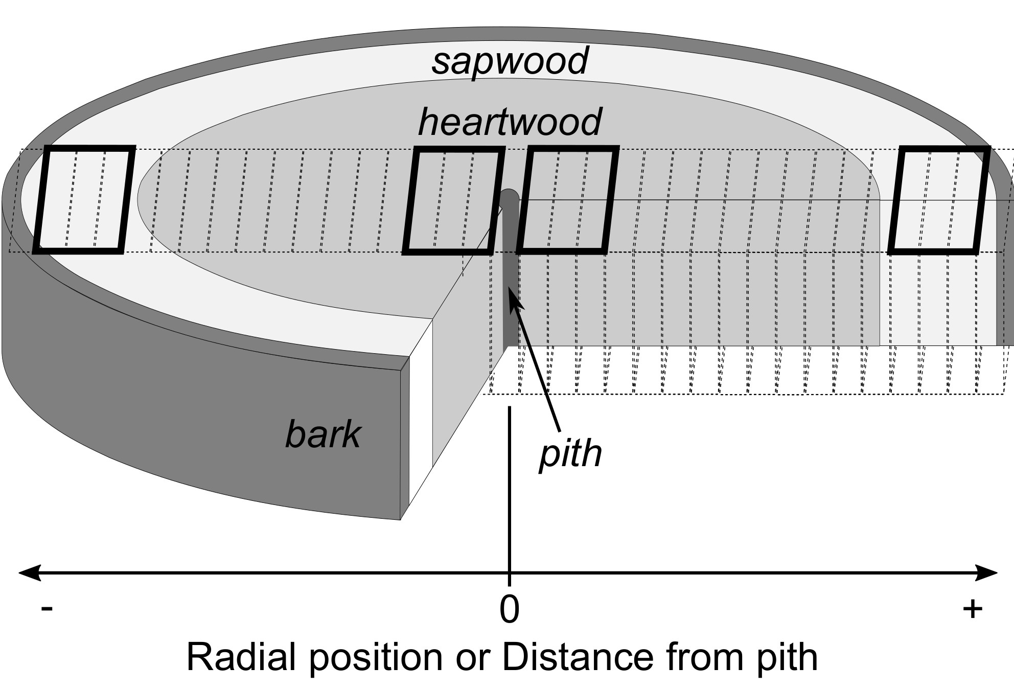
2.5. Assignment of Radial Positions and Measurement of Wood Density

One diametric (i.e., bark to bark through the pith) 2–3 cm wide wood sample, was extracted from each wood disc using a band saw. Each diametric sample was then tangentially cut into 0.5 cm segments from bark to bark, taking care to include pith in one of the segments. Bark segments were discarded. Each wood segment was numbered and assigned to a radial position (i.e., distance from the pith in cm) with the segment containing pith assigned to the central position (i.e., 0 cm). Negative positions were assigned to one side of the disc and positive positions to the other side. For each segment, we determined the nature of the tissue with the naked eye (i.e., bark, HW, SW, and pith) (Figure 1). When a segment contained both HW and SW, it was classified as a HW-SW mixed segment. Inner segments were attributed to HW when their color clearly contrasted with outer segments. The green volume of each segment was measured using the buoyancy (G) of the sample, i.e., G = weight in air (W_a)−submerged weight (W_fl). The mass of the samples was then stabilized in the oven at 103 °C for 48 h and dry mass was recorded (W_d). Both measurements were made using a YDK03 density kit (Sartorius, Goettingen, Germany) and a CP224S 0.2 mg precision balance (Sartorius, Goettingen, Germany). WD was computed as the ratio of dry mass to green volume [1], i.e., W_d/(W_a − W_fl) or W_d/G.

2.6. Comparisons of the Inner, Outer, and Overall Wood Density at Species Level

For each species, we established the inner and outer WD distributions (i.e., _inWD and _outWD) by pooling the 6 innermost and 6 outermost WD values of each tree (3 per radius), respectively (Figure 1). In the present study, the term ‘inner-wood’ may refer to SW or HW, depending on the presence or absence of a distinct visual difference between HW and SW, whereas ‘outer-wood’ refers exclusively to the outermost SW. The species overall WD distribution was established by pooling all WD values. We then compared the overall WD distributions among species using a Kruskal–Wallis test followed by a post-hoc Tukey’s range test. Within each species, _outWD and inner _innWD distributions were also compared using a Kruskal–Wallis test. All statistical analyses in this study were performed using R statistical software [48]. We also computed the species overall WD (WD_mean) as the arithmetic mean of all WD values measured on both radii, after removing samples containing the pith. For a list of variables used in this study and their abbreviations, see

Table 2. List of variables measured and their abbreviations.

WD, HWD, SWD	Wood density, heartwood density and sapwood density (g cm−3)
WDmean, corWDmean	Observed and corrected mean wood density (g cm−3)
WDctr, corWDctr	Observed and corrected wood density at the stem center (g cm−3)
WDgrad, corWDgrad	Observed and corrected wood density radial gradient (g cm−3 m−1)
innWD, outWD	Inner and outer wood density distribution (g cm−3)
RGR95, sRGR95	95th percentile of the radial growth rate distribution of mature tree and sapling (cm year−1)
sMR	Sapling mortality rate (Proportion of dead saplings per year)

.

2.7. Decoupling the Effect of Xylogenesis from that of Heartwood Formation on WD

In order to separate the effects of wood formation and HW extractives production on WD, we estimated the WD produced by young trees (i.e., HW-free inner wood), by (1) carrying out a WD correction based on preexisting or newly acquired chemical data as well as (2) the collection and measurement of WD in young individuals of a subset of 3 species.

2.8. Estimation of Wood Density Corrected by Extractive Content

We computed WD corrected by extractive content (corWD) of HW samples for species showing HW. As the deposition of extractives within the cell wall during HW formation increases the wood mass, corWD was computed as the ratio of corrected dry mass (cW_d) to green volume (G). cW_d was computed using extractive content (extractive mass per wood dry mass) at the species level originating from several kinds of sources (Table S1). The main source was the CIRAD (French agricultural research and international cooperation organization) wood chemistry database (CIRAD, unpublished), which contains 35,823 entries from 671 taxa (577 identified to the species level). We also used a few published studies that addressed specific questions regarding the HW natural durability and extractive content in the species selected for the present study (Table S1). As extractive content data were unavailable for Zygia tetragona Barneby & J.W. Grimes, we proceeded to conduct chemical extraction in water and methanol from HW powder using the same methodology as the CIRAD wood chemistry database (methodology of the Centre Technique Forestier Tropical (CTFT)) (Appendix A, for details on methods and results) to measure extractives content and used this value to compute corWD for this species. We also computed the species overall corrected WD (corWD_mean) as the arithmetic mean by pooling all corWD values from HW and all WD values from SW values, after removing samples corresponding to bark and pith.

2.9. Selected Young Trees of Three Species

Another possible way to analyze the effect of HW extractives on WD variations would be to compare the WD radial profiles of individuals in which HW formation has not yet started with trees where HW is present and clearly demarcated. However, the timing or size that triggers the HW formation process depends on the species and/or the growth environment [36,49], so there is no general rule to enable the selection of trees of sufficient size (i.e., showing significant variations in WD) that do not contain HW. Nonetheless, we decided to compare the sapwood density (SWD) of the trees described above with SWD collected from younger/smaller trees that are likely to not contain HW, or at the most, only very small amounts.

Three species—Bocoa prouacensis Aubl., Eperua grandiflora (Aubl.) Benth., and Zygia tetragona—were compared using 3 to 4 individuals per species whose DBH ranged from 2.5 to 7.5. As explained above, we measured the WD radial profiles of these smaller trees at 0.5 m in order to compare them with radial patterns of bigger trees measured at the same height.

2.10. Successional Status and Demographic Variables

Successional status and demographic data for each species sampled were gathered from different kinds of sources. For the successional status of each species, we used the Favrichon [47] classification, established on the Paracou experimental site, which defined 3 classes of species along the shade-tolerance continuum: heliophilic, semi-tolerant, and shade-tolerant species (Table 1). Successional groups were determined by Favrichon [47] through mutltivariate analysis and classifications with mean diameter, proportion of recruits (tree with DBH >10 cm), and annual growth rate for both natural and perturbed forest at the species level as input variables. In order to link the different WD variables to demographic variables of both mature trees and saplings, we used data available from different census protocols. For mature trees, we used data from the GUYAFOR network database (Guyafor, DataBase of the French Guiana Permanent Plot Network, CIRAD-CNRS-ONF) in order to compute the maximal radial growth rate (in cm/year) and the maximum DBH for each species (DBHmax). The maximal radial growth rate was computed as the 95th percentile of the radial growth rate distribution (RGR95) containing the RGR of each tree averaged over a 30-year period. Data were restricted to the Paracou experimental site in order to avoid potential biases due to differences between sites. For juvenile trees, as the GUYAFOR census protocol considers only individual trees with a DBH greater than 10 cm, the variables for the saplings were computed using two data inventories provided by Molino and Sabatier [50] and Vincent et al. [51]. Between 1995 and 1997, Molino and Sabatier [50] conducted a census, measured and identified all trees with a DBH ranging from 2 to 10 cm, over ten 20 × 250 m transects at Paracou. Vincent et al. [51] recorded mortality events along the same transects, and measured the DBH of the saplings that remained in 2002. From these two measurements, we computed the sapling maximal radial growth rate (sRGR95) at the species level in the same way as for the mature trees of the GUYAFOR network. Molino and Sabatier [50] and Vincent et al. [51] data inventories, were also used to compute the sapling mortality rate (sMR) as the proportion of the number of dead saplings divided by the mean period between the two censuses. To avoid bias due to small sample size, species for which RGR95, sRGR95, and sMR was computed using fewer than 20 individuals were discarded. As a result, among the 16 species used for WD measurements; the sRGR95 and sMR values of 6 species were discarded and the RGR95 values of 2 species were discarded. For a list of variables used in this study and their abbreviations, see Table 2.

2.11. Modeling the Radial Pattern

The WD radial variations of the SW and HW in the sampled individuals were modeled at the species-level using multilevel linear mixed effect models [52]. These models enable integration of random factor effects that may significantly impact estimation of the model parameters and its significance. As variations in WD along the pith-to-bark radius are a common feature of tropical trees, we used distance from the pith as a fixed effect and selected 2 nested random factor levels to allow radial variations in WD to be modeled at different scales in the same species. These 2 nested random factors levels were (1) the individual and (2) the measured pith-to-bark radius within an individual.

As curvilinear patterns exist [20,34], we extended our modeling approach to include quadratic expressions.

In this way, we specified both linear and quadratic full multilevel mixed-effects models, for whom all terms have a random effect at all nested levels considered. Let WD_ijk be the WD value of the kth 0.5 cm interval from the pith of the jth pith-to-bark radius within the ith individual, our full species-level models, in the linear (Equation (1)) and quadratic (Equation (2)) forms, respectively, are expressed as follows.

WD_ijk = (β₀ + β_0i + β_0ij) + (β₁ + β_1i + β_1ij)*x_d + ε_ijk,

(1)

WD_ijk = (β₀ + β_0i + β_0ij) + (β₁ + β_1i + β_1ij)*x_d + (β₂ + β_2i + β_2ij)*x_d² + ε_ijk,

(2)

with x corresponding to the distance from the pith and ε_ijk corresponding to the within group error.

We also specified two mean models (i.e., no radial distance effect), that include (Equation (3)) or do not include (Equation (4)) an individual random effect, in order to highlights species with no significant radial gradient:

WD_ik = (β₀ + β_0i + β_0ij) + ε_ijk,

(3)

WD_ijk = β₀ + ε_ijk,

(4)

2.12. Model Selection Procedure

To evaluate the most suitable model, both quadratic (Equation (1)) and linear models (Equation (2)) were derived in 2 sets of reduced models varying by the inclusion of the different random error terms (7 models per form including the full model of each form). Next, all these models and the two mean models (Equations (3) and (4)) were fitted to the species-level data. All the candidate models were compared with the corrected Akaike Information Criterion (AICc) [53], available in the ‘AICcmodavg’ R package (2.1-1) [54], penalizing models with more parameters in order to keep the most parsimonious and suitable model for each species. We then computed differences between the lowest AICc and the AICc of each model. We only considered fits with the lowest AICc and fits for which AICc differences did not exceed 2, as candidate models. For each candidate model, we checked (1) the validity of linear-mixed model assumptions by graphical examination of residuals [52] and (2) the significance of the fixed effects. Finally, we selected the model with the lowest parameters numbers that did not violate model assumptions and with significant fixed effects. Log-likelihood ratio tests were performed to compare nested models (i.e., models that differ only by the inclusion of one or several random effects) and to check the significance of the inclusion of random effects.

2.13. Determination of the Species Corrected WD Radial Pattern

The corrected WD radial pattern of each species was determined following the modeling procedure. The determination of the corrected WD radial pattern is straightforward for species without HW (i.e., one single fit per radius), but is not for HW-species for which we modeled separately HWD and SWD. Thus, for HW-species we fitted simple linear and quadratic regressions over WD data compounded by SWD values and corrected HWD values and applied the same procedure as explained above. Three types of qualitative patterns were determined based on the mathematical form of the selected model: “linear” for linear form, “upward curvilinear” for quadratic form with β₁ < 0 and β₂ > 0, and “downward curvilinear” for quadratic form with β₁ > 0 and β₂ < 0.

2.14. Calculation of Observed and Corrected Radial Gradients

Based on the modeling of radial patterns, we computed the observed WD radial gradient of each species (i.e., the change in WD per radius unit) as

WD_grad = (WD_x − WD_ctr)/x, in g cm⁻³ m⁻¹,

(5)

where WD_ctr equals the WD at the stem center (i.e., the estimation of β₀ from the whole stem or HW modeling of HW-free and HW species, respectively) and WD_x refers to the predicted WD at the radial distance x in m. Here, we chose x = 0.06 m because this was the outermost value covered by all the species sampled in this study. The corrected radial gradient of each species was computed as

corWD_grad = (WD_x − corWD_ctr)/x, in g cm⁻³ m⁻¹,

(6)

with corWD_ctr equal to the corrected WD at stem center.

For species for which both mature trees and saplings were collected, we used the intercept estimated from sapling modeling as corWD_ctr. When no saplings were collected, we used the intercept estimated from SWD modeling after checking the consistency between this parameter and the observed range of WD at the stem center corrected by extractive content. The corrected WD gradient (corWD_grad) was not computed for species whose extractive contents were not available.

2.15. Correlations among WD Variables and between WD Variables and Demographic Variables

We then proceeded to correlations among WD variables (i.e., WD_mean, corWD_mean, WD_ctr, corWD_ctr, WD_grad, and corWD_grad) and between WD variables and demographic variables (i.e., RGR95, sRGR95, sMR, and DBHmax). After checking the normality of these variables, we used the Pearson correlation with the rcorr() function implemented in the ‘Hmisc’ package (4.1-1) [55]. The significance of each correlation coefficient was assessed by the p-value provided by the rcorr() function.

2.16. Linking Successional Status and Corrected WD Radial Pattern to WD and Demographic Variables

Significant differences between both WD and demographic variables and successional status and corrected WD radial pattern were assessed using the Kruskal–Wallis rank test followed by a post-hoc Tukey honest significant differences test when significant differences were revealed by the Kruskal–Wallis test. Kruskal–Wallis and Tukey tests were performed using ‘base’ (3.6.0) [48] and ‘agricolae’ (1.3-0) R packages [56], respectively.

3. Results

3.1. Observed Overall, Inner and Outer Wood Density at the Species Level

Our sampling covered a wide range of WD values at both sample level (0.186 in P. nitida Miq. to 1.156 g cm⁻³ in B. prouacensis) and species level (0.304 in P. nitida to 1.055 g cm⁻³ in Z. tetragona). The observed range of WD was continuously covered by the 16 selected species (Figure 2). Species with low overall WD exhibited lower _innWD than _outWD, and inversely, species with high overall WD exhibits higher _innWD than _outWD. Interestingly, species in which _innWD > _outWD all exhibited clearly demarcated HW, apart from V. Americana Aubl., for which no significant differences between _innWD and _outWD were observed. However, species in which _innWD < _outWD are both HW-free and HW species. T. guianensis (Benth.) Zarucchi & Herend. was the only HW-free species that exhibited no differences between _innWD and _outWD (Figure 2).

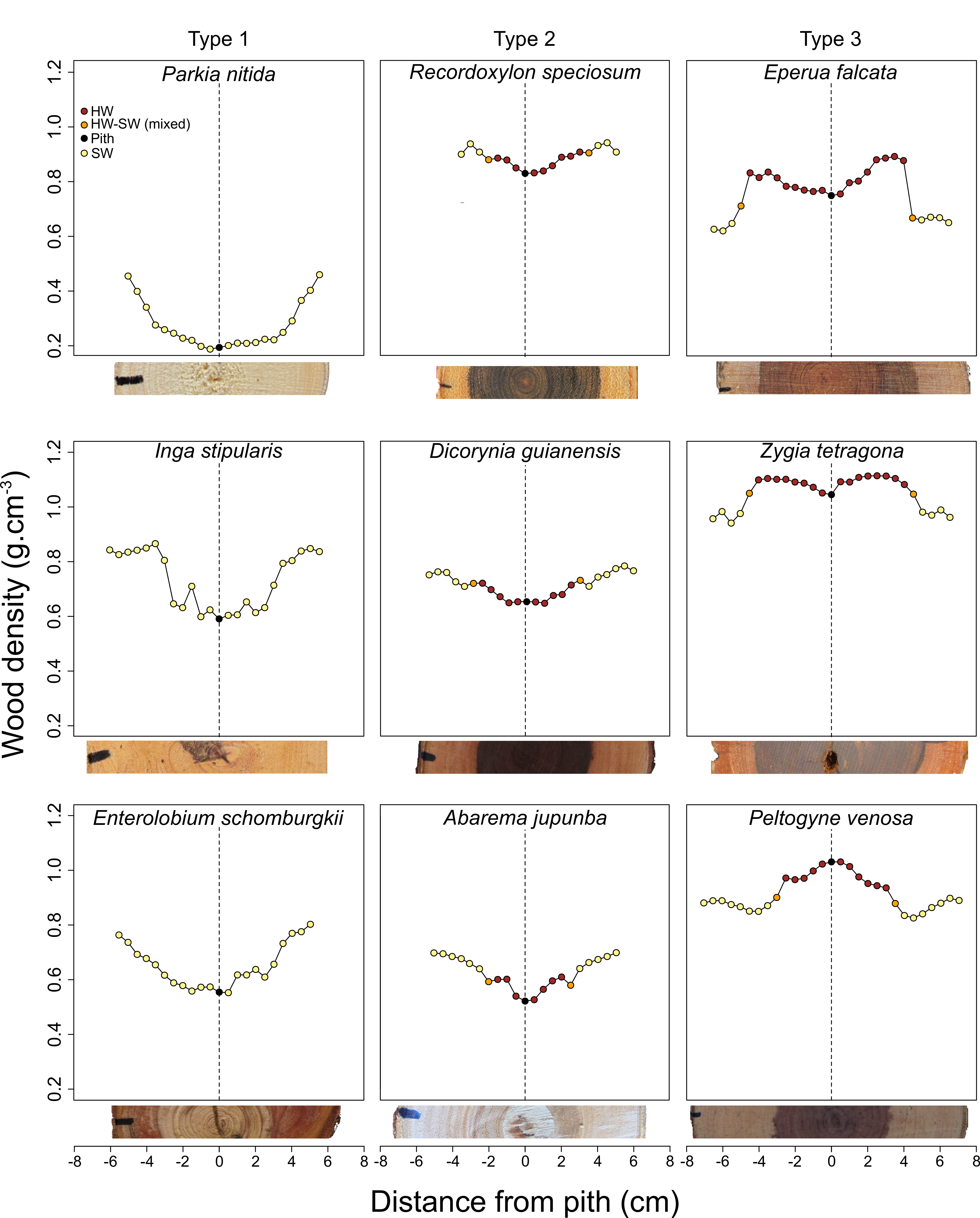
3.2. Qualitative Assessment of WD Radial Patterns in Light of the Presence of Heartwood

Taking the presence of HW into account, the observation of variations in WD from the pith to the bark enabled three qualitative types of radial patterns to be distinguished (Figure 3) resulting in the above-mentioned differences between _innWD and _outWD (Figure 2). Type 1 was represented by species with no HW in which WD increased from the pith to the bark (e.g., P. velutina Benoist, P. pendula (Willd.) Walp., P. nitida, I. stipularis DC., and E. schomburgkii (Benth.) Benth.). Type 2 corresponded to species with HW in which WD increased from the pith to the bark (e.g., R. speciosum (Benoist) Gazel ex Barneby and A. jupunba (Willd.) Britton & Killip). Type 3 corresponded to species with HW in which the HWD was higher than SWD (E. falcata, E.grandiflora, B. prouacensis, and Z. tetragona). Taking into account the presence of HW and SW highlights the effect of HW on WD radial changes (Figure 3). Indeed, among Type 3 species, a sharp decrease in WD occurred at the HW-SW transition. The WD values of mixed type samples (i.e., samples made of SW and HW) were often intermediates to samples containing either only SW or only HW. In Type 2 species, the WD of mixed type samples was lower than that of the adjacent HW samples.

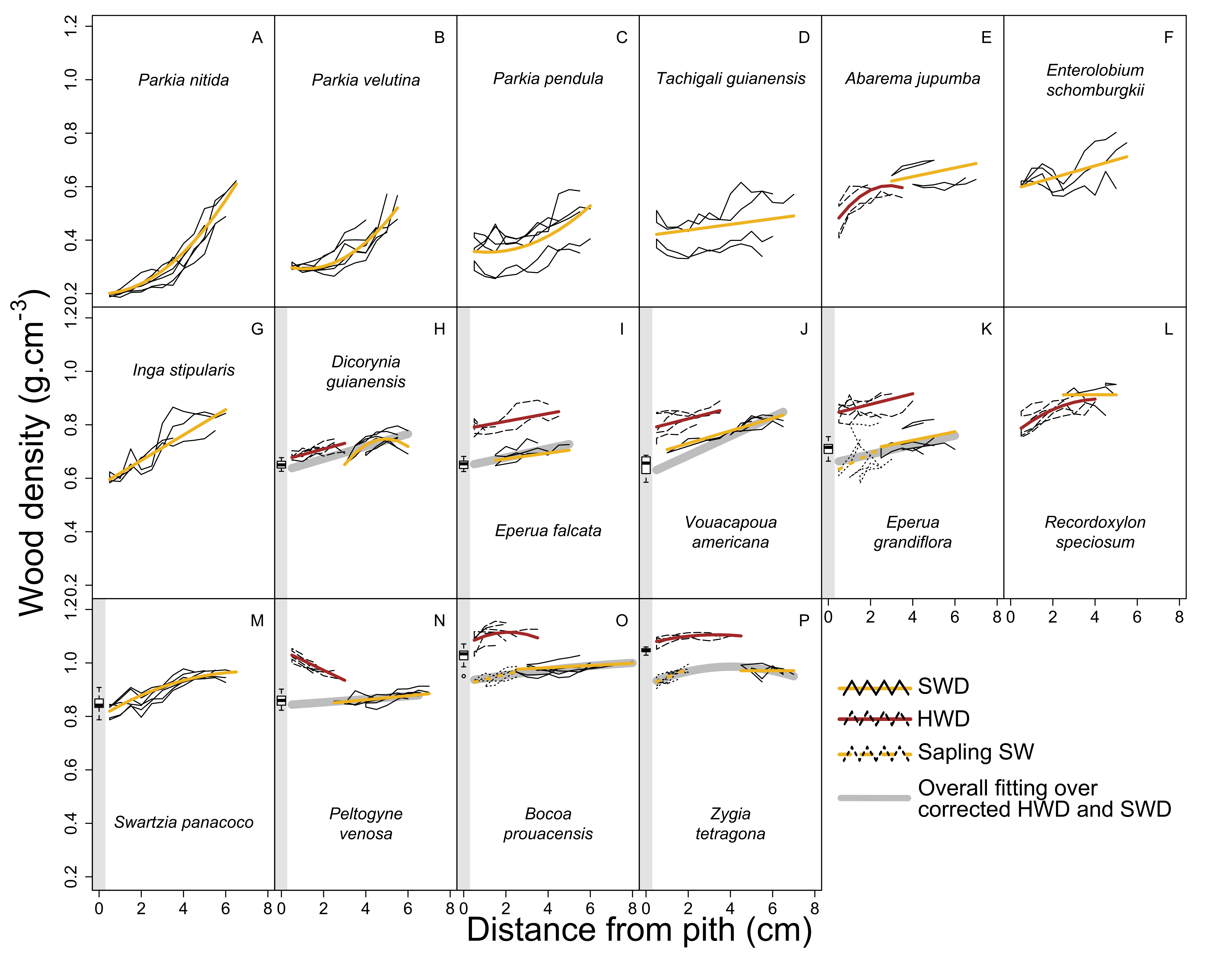
3.3. Modeling of WD Radial Variation in Heartwood and Sapwood

Modeling the radial variations of WD reveals that HW-free species exhibit exclusively positive radial patterns (Figure 4A–D,F,G,M). Three out of the seven species have an upward curvilinear pattern (i.e., the slope increases with increasing distance from the pith; Figure 4A–C) whereas three others have linear patterns (Figure 4D,F,G) and one has a downward curvilinear pattern (i.e., the slope decreases with increasing distance from the pith; Figure 4M). Among the species with HW, A. jupunba, D. guianensis Amshoff and R. speciosum only show a slight decrease in WD at the HW/SW boundary (Figure 4E,H,L) resulting in an almost continuous downward curvilinear pattern. In these three species, HWD increases significantly, whereas SWD only varies significantly in A. jupunba and D. guianensis (Figure 4E,L, respectively). In the others species with HW, a marked decrease in WD can be seen at the HW/SW boundary (Figure 4I–K,N–P). In V. americana, E. falcata, and E. grandiflora (Figure 4I–K), both SWD and HWD increase linearly. In B. prouacensis and Z. tetragona (Figure 4O,P), there is a significant downward curvilinear pattern in HW, whereas SWD increases linearly in B. prouacensis and is constant in Z. tetragona. P. venosa (M.Vahl)Benth. is the only one species with a significant pattern inversion between SW and HW with decreasing and increasing HWD and SWD, respectively (Figure 4N). The range of corrected inner WD and the estimation of WDctr by modeling SWD variations of bigger individuals (i.e., the value of the intercept β₀, see Table S2) are in partial agreement for V. americana, P. venosa, E. falcata, and E. grandiflora, the estimation of β₀ is in the range of corrected inner WD, whereas for B. prouacensis, Z. tetragona, and D. guianensis, estimated β₀ is below the observed range (the description of the selected models is available in Table S2. The statistics of all the fitted models are given in Table S3).

3.4. Effect of Extractives in Bocoa prouacensis, Zygia tetragona, and Eperua falcata

Interestingly, the juxtaposition of the SWD modeled patterns of saplings and larger trees produces remarkably continuous tendencies across the whole radius (Figure 4N–P). Modeling of SWD variations in young trees reveals only positive linear patterns of variation in the three species considered. A new comparison between the ranges of corrected _innWD and the estimation of WD_ctr by modeling SWD variations on saplings (i.e., the value of the intercept β₀, see Table S4) shows that the estimation of β₀ lies far below the corrected _innWD range for these three species (Figure 4N–P).

3.5. Observed and Corrected Radial Gradient

The observed radial gradient (WD_grad) varies from −2.74 to 5.84 g cm⁻³ m⁻¹ in P. venosa and P. nitida, respectively, with an average value of 1.82 g cm⁻³ m⁻¹ (Table S3). The computation of the corrected radial gradient (corWD_grad) only resulted in positive gradients with the lowest expressed by P. venosa (i.e., corWD_grad = 0.75 g cm⁻³ m⁻¹) and increase the average value to 2.75 g cm⁻³ m⁻¹.

3.6. Correlations among WD Variables and between WD Variables and Demographic Variables

Significant correlations among WD variables are observed (

Table 3. Pearson correlations among WD variables and between WD variables and demographic parameters.

	WD Variables					Demographic Variables
	corWDmean	WDctr	corWDctr	WDgrad	corWDgrad	RGR95	sRGR95	sMR	DBHmax
WDmean	0.99 ***	0.96 ***	0.99 ***	−0.66 ***	−0.56 ***	−0.86 ***	−0.61	−0.47	−0.34
corWDmean		0.94 ***	0.98 ***	−0.61 ***	−0.54 ***	−0.85 ***	−0.57	−0.45	−0.38
WDctr			0.97 ***	−0.83 ***	−0.69 ***	−0.88 ***	−0.69 ***	−0.42	−0.22
corWDctr				−0.74 ***	−0.66 ***	−0.91 ***	−0.79 ***	−0.71 ***	−0.28
WDgrad					0.91 ***	0.66 ***	0.56	0.32	−0.11
corWDgrad						0.65 ***	0.69	0.41	−0.16

Stars indicate the level of significance for each Spearman coefficient (*** <0.001); WDmean and corWDmean, uncorrected and corrected mean WD; WDctr and corWDctr, uncorrected and corrected mean WD at the stem center; WDgrad and corWDgrad, uncorrected and corrected WD gradient; RGR95, 95th percentile of mature tree radial growth rate; sRGR95, 95th percentile of saplings radial growth rate; sMR, sapling mortality rate; DBH, maximal DBH value.

). Whereas uncorrected and corrected mean WD and WD at the stem center (i.e., WD_mean, corWD_mean, WD_ctr, and corWD_ctr) are highly positively correlated (r > 0.95), these three variables are negatively correlated with the uncorrected WD gradient (WD_grad) suggesting that the higher the averaged WD variables, the lower the value of WD_grad. However, although still significant, the correlations between corWD_grad and other WD variables are weaker.

Regarding demographic variables, WD variables are significantly correlated with RGR95 and sRGR95. The higher the values of WD_mean, corWD_mean, WD_ctr, and cWD_ctr, the lower the values of both RGR95 and sRGR95, although negative correlations between sRGR95 with WD_mean, corWD_mean, WD_grad, and cWD_grad are marginally significant. However, no significant correlation is apparent between DBHmax and WD variables. Regarding sMR only a significant negative correlation with cWD_ctr is apparent, while interestingly, sMR is not significantly correlated with WD_ctr.

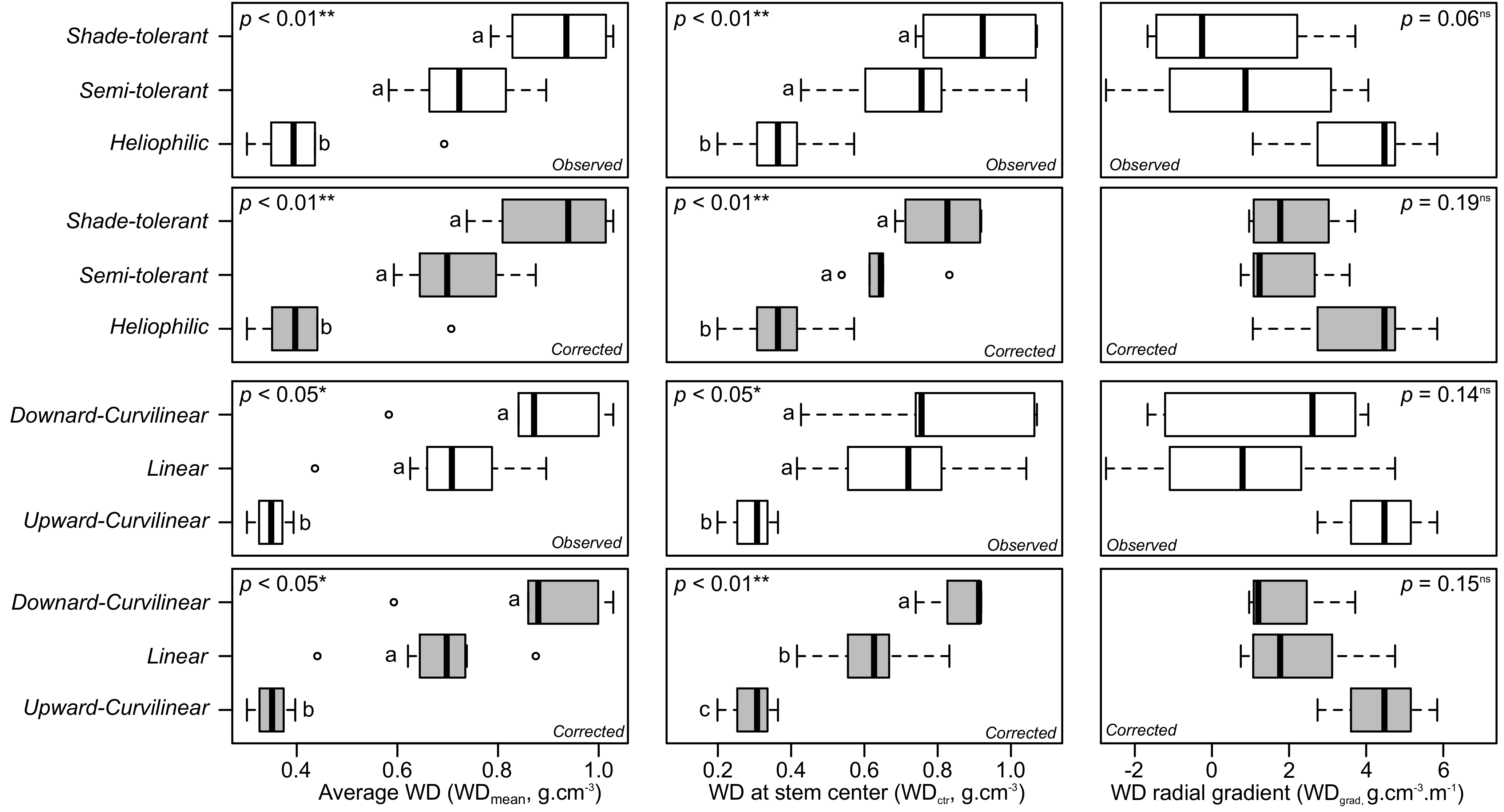
3.7. Links between WD Variables, WD Profile, and Successional Status

Both observed and corrected species-average WD, as well as WDctr, differed significantly according to the shade tolerance index (Figure 5, upper panel). Values for heliophilic species were significantly lower than those of semi-tolerant and shade-tolerant species for these variables. Despite the systematically higher average values observed for shade-tolerant species (Table S5), we did not detect any significant differences between shade-tolerant species and semi-tolerant species (Figure 5, upper panel). Neither WD_grad nor corWD_grad showed any significant differences between shade tolerance indexes (Figure 5, upper panel).

The same tendencies emerged when distinguishing the different types of radial pattern using the WD variables (Figure 5, lower panel). For this comparison, we classified our species in three groups of corrected radial pattern by visual examination of the radial tendencies (Figure 4): (1) upward curvilinear pattern (i.e., P. nitida, P. velutina Benoist, and P. pendula); (2) linear (i.e., T. guianensis, E. schomburgkii (Benth.)Benth., I. stipularis, D. guianensis, E. falcata, E. grandiflora, V. americana, and P. venosa); and (3) downward curvilinear pattern (i.e., A. jupumba, R. speciosum, S. panacoco (Aubl.) Cowan, B. prouacensis, and Z. tetragona). Species with an upward curvilinear pattern showed the lowest value of both WDmean and corWDmean, as well as WDctr and corWDctr whereas species with a downward curvilinear pattern showed the highest. Again, despite systematically higher averages values observed for species with a curvilinear downward pattern (Table S5) we did not observe any significant differences between species with a curvilinear pattern and species with a linear pattern (Figure 5, lower panel).

The same analysis performed with demographic variables instead of variables related to WD, led to significant differences in RGR95 and sMR between shade-tolerance indexes (Table S5). Heliophilic species had the highest RGR95 and sMR, whereas shade tolerant species had lower values for these variables; semi-tolerant species were between the two extremes. More surprisingly, we did not detect any significant differences between shade tolerance indexes according to sRGR95 or DBHmax. When conducting the same analysis according to WD radial patterns, we did not find any significant differences (Table S5).

4. Discussion

Through the combination of fine-scale analysis of WD variation, demographic data, and HW extractive content value, our study (1) underlines the risks of functional misinterpretation of WD radial variation when WD is not corrected by HW extractives content value, (2) proposes a classification of corrected WD along the shade-tolerance continuum that enables avoiding this bias, and (3) highlights the functional significance of corrected WD value at the stem center.

4.1. The Effect of HW Extractives Impregnation on Wood Density Radial Gradients and Possible Functional Misinterpretation Due to Uncorrected Wood Density

We differentiate three qualitative types of WD patterns regarding the occurrence of HW and the differences between _innWD and _outWD (Figure 3). Type 1 is HW-free and exhibits higher _outWD than _innWD. However this trend is also observed in Type 2 species with HW. While the non-consideration of HW in these two types will lead to the same qualitative evaluation of WD variation (i.e., greater under the bark than at the center of the stem), from a quantitative point of view, the radial gradient in Type 2 species will be biased by the production of HW and underestimated. However, since the HW formation process increases the mass of the wood through extractives synthesis, the failure to take the presence of HW into account only affects the magnitude of the gradient but not its direction in that case. This statement does not hold for Type 3 species with both HW and a greater WD at the stem center than under the bark. This result confirms the effect of HW on WD radial variations already suspected by several authors [26,33]. Here, prior knowledge of WD value before HW formation is needed or can be estimated trough WD correction or by sampling young individuals in which HW formation has not started yet. Such information is indispensable to differentiate both the direction and the magnitude of the radial gradient attributable to xylogenesis alone from the gradient attributable to both xylogenesis and HW formation and to accurately relate WD radial pattern to tree growth strategy.

4.2. On the Corrected Radial Gradient, Patterns and Their Link with Overall, Inner/Outer WD, and the Shade-Tolerance Continuum

After correction of the WD using the concentration of extractives, our analysis revealed that all the species we sampled exhibited a positive WD radial gradient ranging from very strong (e.g., Parkia genus representatives) to very slight (e.g., B. prouacensis and Z. tetragona) (Figure 5). These findings contrast with the bulk of studies on WD radial variations [26,29,32,33,34,35], which reported both negative and positive gradients. We presume that this difference is mainly due to the failure to take into account the presence of HW that was previously hypothesized by several authors [26,33]. Another important effect could be related to the size and the ontogenetic stage reached by the individuals sampled, this aspect will be discussed in the last section of the discussion.

Our modeling of the corrected WD variation according to distance from the pith, revealed three different types of radial patterns: (1) an upward curvilinear pattern in species with the lowest overall WD as well as the lowest WD at the stem center (WD_ctr); (2) a linear pattern in species with an intermediate to high WD (according to observed and corrected overall WD and WD_ctr), but that occurs in a wide range of WD gradients; and (3) a downward curvilinear pattern mainly observed in species with very dense wood and in those with the least radial variations.

Despite the nonsignificant differences in corrected WD radial gradients between the different types of radial patterns (Figure 5), the highest WD gradients were observed among species with the upward curvilinear pattern. This recently described pattern of WD variation [20,34,57], in fact appears to be relatively common.

The striking agreement between the distributions of the radial pattern on one hand and the index of tolerance on the other hand, according to WD variables (Figure 5), led us to characterize the relationships between these two criteria. In the 16 species in which we clearly identified the type of radial pattern: (1) the upward curvilinear pattern (i.e., three species) was only represented by heliophilic species; (2) the linear pattern was mostly represented by species with early to intermediate successional characteristics (i.e., two heliophilic and five semi-tolerant), V. americana being the only shade-tolerant species with a linear pattern; (3) the downward curvilinear pattern was represented by species with intermediate to late successional characteristics (i.e., two semi-tolerant and three shade-tolerant species) (Figure 4 and Figure 5). Therefore, the gradual change in the corrected WD radial patterns, i.e., from upward to downward curvilinear via a linear pattern illustrates a gradual change in species-successional characteristics. Such findings provide a coherent framework for the inference of biomass allocation and mechanical strategies of establishing trees along the shade tolerance continuum (Figure 6).

4.3. Do Low WD Gradients Only Illustrate Late-Successional Species?

Although we did not find any negative WD radial gradients, our study corroborates a common scheme of decreasing WD radial gradient from early to late-successional species [25,29]. Here, the following elements could explain this observation. Saplings of early-successional species exhibit high height growth rate [57,58,59]. This high investment in height growth should be achieved by the production of low WD at stem center. Thus, differential carbon allocation strategy between height growth and stem thickening represents a competitive advantage during the early stages. As height growth rate decreases from early to late successional species [59], we expect that such a difference in carbon investment between height growth and stem thickening during the early stages should be less pronounced in mid and late-successional species. This hypothesis agreed with the decreasing WD radial gradient and the increasing WD at stem center observed from early to late-successional species. However, it is important to note some deviations from this common scheme. Indeed, not only late-successional species have an almost constant WD from pith to bark. In our sample, T. guianensis, exhibited a significant but quite low WD gradient (i.e., 0.9 g cm⁻³.m⁻¹). Therefore we can speculate that the evolutionary history of this species favored a strategy that made it possible to achieve sufficient mechanical strength, at least by young individuals, with the same carbon investment, through the production of a larger but less dense stem [60,61]. However, this alternative strategy to the common pith-to-bark increase in WD, would be expected to increase the maintenance cost associated with the higher amount of bark and wood tissues [61]. The reduction in maintenance cost achieved by reducing the stem area is probably the main evolutionary driver of the common occurrence of a WD gradient. Reciprocally, given the negative correlation between WD and water storage [8,62], very low and almost invariable WD can be seen as an adaptive strategy of succulent-stem species, such as the African Baobab (Adansonia spp., Malvaceae) [63], at the cost of higher maintenance requirements. Interestingly, other representatives of the family Malvaceae in the Neotropics contain almost constant and very low density wood [24,25]. Given the above-mentioned functional trade-off between WD and water storage ability, it is important to emphasize the possible effect of wood multifunctionality as a driver of WD gradient magnitude.

4.4. Limitations to the Correction of WD by Extractive Content

The use of species-level extractive content to compute the corrected WD proved to be very useful to describe and understand WD variation exclusively produced by xylogenesis. Nevertheless, the partial agreement between the range of corrected _innWD and the estimation of WD_ctr by modeling SWD variations revealed some limitations concerning this method.

First, from a mathematical point of view, it is important to mention that the parameters extrapolated from the polynomial model are not based on the true behavior of the data, thus more confidence should be placed in the interpretation of corrected WD_ctr estimated from linear modeling than from polynomial modeling. For instance, polynomial modeling of SWD variation in D. guianensis—the most exploited timber species in French Guiana—produced a too low estimate of WD_ctr, i.e., 0.12 g cm⁻³, to be considered as a plausible value. A linear model fitted on the whole D. guianensis SW data provided a plausible WD_ctr value of 0.645 g cm⁻³. Except for this consideration, the disagreement between the ranges of corrected _innWD and extrapolated corrected WD_ctr might result from intraspecific variability, which might not be sufficiently covered given the insufficient number of individuals sampled in the CIRAD wood chemistry database (Table S1). Moreover, HW extractives are known to vary radially within the same individual [64,65,66,67,68], which is supported by the observed radial variation of wood natural durability within the same individual [69], but might also vary positively or negatively from pith to bark depending on the species considered [64,70] or on the type of extractive [65,66,67]. Given the agreement between the range of corrected _innWD and the estimation of corWD_ctr observed in P. venosa, we hypothesize that the decrease in the HWD from the pith to the HW/SW boundary might be due to the decrease in total extractive content. Finally, SW also contains extra material such as nonstructural carbohydrates, gums, resins, silicate, or precursors of extractives [37,49,71,72] that may impact SWD. Although it is generally acknowledged that the concentration of extra materials is generally lower in SW than in HW [70], some species may have high extractive content in the SW [36,72]. In this sense SWD should also be corrected by extra-material content.

4.5. WD Variations and Demographic Variables

Our results confirm the negative relationship between the radial growth rate and averaged WD of both saplings and mature trees [2,14,73]. Correlations involving sRGR95 and averaged WD are weaker and marginally significant compared with correlations involving RGR95 except for both corrected and uncorrected WD at the stem center (corWD_ctr and WD_ctr). Interestingly, we found a better correlation between sRGR95 and corWD_ctr than between sRGR95 and WD_ctr. As it seems very likely that the HW formation process has not yet started in saplings, this result could be explained by the fact that it is more relevant to compare the growth rate of an individual and the wood it produces at the same time. It is generally acknowledged that high WD density at the stem center enables saplings to resist falling objects thanks to their high mechanical strength [3,6] and high natural durability [4,30]. Thus, in the same line of thought as above, it should be more relevant to link the sapling mortality rate (sMR) to the corWD_ctr. Again, both the significant correlation between sMR and corWD_ctr and the nonsignificant correlation between sMR and WD_ctr stress the relevance of corWD_ctr in predicting sapling mortality rate. This result agrees with the recent study of Osazuwa-Peters et al. [46], reporting a nonsignificant correlation between WD measured close to the pith on mature trees (i.e., uncorrected WD) and sapling mortality rate in 20 species from Barro Colorado Island, Panama. Our results show that the interspecific differences in corWD_ctr are significantly explained by the observed differences in sMR. Thus, the mechanical characteristics required to survive in the understory are achieved by a relatively dense SW. The stiffness of the wood material is mainly provided by the cellulose produced during the cell wall maturation process [74], in this sense the deposition of secondary metabolites during HW formation should not affect the stiffness of the material, even though the opposite results obtained by some authors make the effect of extractives on mechanical properties a controversial topic [75]. Moreover, an increase of mass around the neutral axis of the stem is not of particular interest as bending stresses are exerted on the outer wood. Cellulose microfibril angle and fiber organization are also correlated with the stiffness of wood [76,77,78], underlining that WD should not be considered as the unique driver of wood stiffness.

Since HW is absent or poorly developed in sapling stems, we would also expect that the protective function of the HW is not effective but can be provided by extractives (or the secondary metabolites) produced by parenchyma cells and stored in the SW [49,79,80]. It is noteworthy that HW natural durability is mainly afforded by extractives content rather than WD alone [81] and that there is not any mechanistic evidence of the role of WD in pest resistance. The positive relationship between pest resistance and WD [4,30] might result from the occurrence of high extractives content in species with dense wood.

These considerations highlight the strong potential of the corrected WD value at the stem center (corWD_ctr) for the inference of sapling functional strategies in a retrospective context. The corWD_ctr should be used as an unbiased proxy of both radial and mortality rates of young individuals instead of the uncorrected WD_ctr. However, this statement only holds for species containing HW, i.e., semi-tolerant to shade-tolerant species. The simple uncorrected WD_ctr can be used for HW-free early successional species. A significant positive correlation was also observed between uncorrected WD gradient (WD_grad) and RGR95, confirming the results of Hietz et al. [33]. Moreover, the nonsignificant differences in the corWD_grad between shade-tolerance indexes confirm that a wide range of corWD_grad can be observed in the same successional class [32] and that corWD_ctr is a better proxy of the species position along the shade tolerance continuum [33].

4.6. What Can We Expect for Wood Density Gradients of Canopy Trees?

Whereas our study reveals that establishing trees present only increasing or constant WD values from the pith to the bark, it is legitimate to question if the same WD gradients and patterns would be valid for mature canopy trees. In the study of WD radial variation on 304 species in Panama and Ecuador, Hietz et al. [33] observed WD radial gradients ranging from −2 to +2.5 g cm⁻³ m⁻¹. Regarding the higher specific diversity sampled by Hietz et al. [33], we would expect a smaller range of WD gradients in our study. However, our range of WD_grad is larger, i.e., −2.74 to 5.84 g cm⁻³ m⁻¹. We assume that this difference originates from the interaction between the size of the sampled tree and the widespread occurrence of a nonlinear WD radial pattern. For species with a downward curvilinear increase, the WD tends to asymptote with an increase in tree diameter. Thus, WD_grad measured on bigger individuals will be lower than WD_grad measured on smaller trees. Nevertheless, this cannot hold for species with an upward curvilinear or linear pattern. For instance, the WD radial gradient of P. nitida and S. panacoco, i.e., 5.84 and 2.78 g cm⁻³ m⁻¹, respectively, would produce WD values under the bark of 4.11 and 1.55 g cm⁻³, respectively, for trees measuring 40 cm DBH, which are beyond the range of possible WD values given that the cell-wall density is approximately 1.5 g cm⁻³ [82]. This highlights the limit of our sampling in the inference of WD patterns for bigger individuals. We might, however, expect that in P. nitida and S. panacoco, the WD value would level off in bigger trees, in turn shifting the radial pattern observed in smaller individuals, as observed in Bagassa guianensis [68]. Thus, bigger individuals of S. panacoco should exhibit a downward curvilinear increase, whereas bigger P. nitida trees should exhibit a sigmoidal radial pattern, i.e., the combination of an upward and downward curvilinear increase not described in our study. This last consideration and the absence of any significant correlation between the maximum diameter of the species (DBHmax) and WD variables of establishing trees, highlight that these variables cannot be linked to, or be predictive of, the maximum size of the species, due to a size-effect already mentioned by Plourde et al. [35].

5. Conclusions

Whereas it was previously considered that late-successional species produce relatively denser wood at the stem center than at the periphery, in order to meet mechanical requirements and to resist pests, our study on the effect of heartwood formation on WD radial gradients in Amazonian leguminous tree species showed an exclusively significant positive pith-to-bark WD gradient.

This finding underlines the importance of considering the effects of extractives on WD to avoid biased interpretations when inferring species’ mechanical strategies. We also point out that even if the early successional species have the strongest positive WD gradients, semi-tolerant species may also exhibit considerable positive variations. Thus, the particular allocation strategy enabling fast height growth followed by the mechanical reinforcement of the structure through the increasing WD from pith to bark is a strategy shared by all species in our sampling, regardless of their shade tolerance characteristics or position along the growth–mortality trade-off, rather than a specific feature of heliophilic species. From a practical point of view, the way that corrected WD varies radially, i.e., the corrected WD radial pattern, could be a relevant indicator of species shade tolerance indexes as a complement to both mean WD and WD gradient. Finally, our study stresses the importance of acknowledging and considering the effect of heartwood when inferring mechanical or other wood-related functions, especially for saplings, when using WD as a proxy in a retrospective approach. A step forward in the understanding of WD variations could be achieved through the integration of both WD and extractives content variation in trees.

References

1. Kollmann, F.F.P.; Côté, W.A. Principles of Wood Science and Technology: I Solid Wood; Springer: Berlin, Germany, 1984. [Google Scholar]
2. Muller-Landau, H.C. Interspecific and inter-site variation in wood specific gravity of tropical trees. Biotropica 2004, 36, 20–32. [Google Scholar] [CrossRef]
3. Van Gelder, H.A.; Poorter, L.; Sterck, F.J. Wood mechanics, allometry, and life-history variation in a tropical rain forest tree community. New Phyt. 2006, 171, 367–378. [Google Scholar] [CrossRef] [PubMed] [Green Version]
4. Chave, J.; Coomes, D.; Jansen, S.; Lewis, S.L.; Swenson, N.G.; Zanne, A.E. Towards a worldwide wood economics spectrum. Ecol. Lett. 2009, 12, 351–366. [Google Scholar] [CrossRef] [PubMed] [Green Version]
5. Wright, S.J.; Kitajima, K.; Kraft, N.J.B.; Reich, P.B.; Wright, I.J.; Bunker, D.E.; Condit, R.; Dalling, J.W.; Davies, S.J.; Díaz, S.; et al. Functional traits and the growth–mortality trade-off in tropical trees. Ecology 2010, 91, 3664–3674. [Google Scholar] [CrossRef] [PubMed]
6. Niklas, K.J. Influence of tissue density-specific mechanical properties on the scaling of plant height. Ann. Bot. 1993, 72, 173–179. [Google Scholar] [CrossRef]
7. Niklas, K.J.; Spatz, H.-C. Worldwide correlations of mechanical properties and green wood density. Am. J. Bot. 2010, 97, 1587–1594. [Google Scholar] [CrossRef] [PubMed] [Green Version]
8. Pratt, R.B.; Jacobsen, A.L.; Ewers, F.W.; Davis, S.D. Relationships among xylem transport, biomechanics and storage in stems and roots of nine Rhamnaceae species of the California chaparral. New Phyt. 2007, 174, 787–798. [Google Scholar] [CrossRef] [Green Version]
9. Lachenbruch, B.; Moore, J.; Evans, R. Radial Variation in Wood Structure and Function in Woody Plants, and Hypotheses for Its Occurrence. In Size- and Age-Related Changes in Tree Structure and Function; Meinzer, F.C., Lachenbruch, B., Dawson, T.E., Eds.; Springer: Berlin, Germany, 2011; Volume 4, pp. 121–164. [Google Scholar]
10. Hacke, U.G.; Sperry, J.S.; Pockman, W.T.; Davis, S.D.; McCulloh, K.A. Trends in wood density and structure are linked to prevention of xylem implosion by negative pressure. Oecologia 2001, 126, 457–461. [Google Scholar] [CrossRef]
11. Markesteijn, L.; Poorter, L.; Paz, H.; Sack, L.; Bongers, F. Ecological differentiation in xylem cavitation resistance is associated with stem and leaf structural traits. Plant Cell Environ. 2011, 34, 137–148. [Google Scholar] [CrossRef]
12. Rosner, S. Wood density as a proxy for vulnerability to cavitation: Size matters. J. Plant Hydraul. 2017, 4, 1–10. [Google Scholar] [CrossRef]
13. Zanne, A.E.; Westoby, M.; Falster, D.S.; Ackerly, D.D.; Loarie, S.R.; Arnold, S.E.J.; Coomes, D.A. Angiosperm wood structure: Global patterns in vessel anatomy and their relation to wood density and potential conductivity. Am. J. Bot. 2010, 97, 207–215. [Google Scholar] [CrossRef] [Green Version]
14. King, D.A.; Davies, S.J.; Tan, S.; Noor, N.S.M. The role of wood density and stem support costs in the growth and mortality of tropical trees. J. Ecol. 2006, 94, 670–680. [Google Scholar] [CrossRef] [Green Version]
15. Poorter, L.; Wright, S.J.; Paz, H.; Ackerly, D.D.; Condit, R.; Ibarra-Manríquez, G.; Harms, K.E.; Licona, J.C.; Martínez-Ramos, M.; Mazer, S.J.; et al. Are functional traits good predictors of demographic rates? Evidence from five neotropical forests. Ecology 2008, 89, 1908–1920. [Google Scholar] [CrossRef] [PubMed]
16. Nascimento, H.E.M.; Laurance, W.F.; Condit, R.; Laurance, S.G.; D’Angelo, S.; Andrade, A.C. Demographic and life-history correlates for Amazonian trees. J. Veg. Sci. 2005, 16, 625–634. [Google Scholar] [CrossRef]
17. Meinzer, F.C.; Lachenbruch, B.; Dawson, T.E. Size- and Age-Related Changes in Tree Structure and Function; Springer: Dordrecht, The Netherlands, 2011. [Google Scholar]
18. Wiemann, M.; Williamson, G. Extreme radial changes in wood specific gravity in some tropical pioneers. Wood Fiber Sci. 1988, 20, 344–349. [Google Scholar]
19. Rueda, R.; Williamson, G.B. Radial and vertical wood specific gravity in Ochroma pyramidale (Cav. ex Lam.) Urb. (Bombacaceae). Biotropica 1992, 24, 512–518. [Google Scholar] [CrossRef]
20. Williamson, G.B.; Wiemann, M.C.; Geaghan, J.P. Radial wood allocation in Schizolobium parahyba. Am. J. Bot. 2012, 99, 1010–1019. [Google Scholar] [CrossRef] [PubMed]
21. Bastin, J.-F.; Fayolle, A.; Tarelkin, Y.; Van den Bulcke, J.; de Haulleville, T.; Mortier, F.; Beeckman, H.; Van Acker, J.; Serckx, A.; Bogaert, J.; et al. Wood specific gravity variations and biomass of central African tree species: The simple choice of the outer wood. PLoS ONE 2015, 10, e0142146. [Google Scholar] [CrossRef] [PubMed]
22. Longuetaud, F.; Mothe, F.; Santenoise, P.; Diop, N.; Dlouha, J.; Fournier, M.; Deleuze, C. Patterns of within-stem variations in wood specific gravity and water content for five temperate tree species. Ann. For. Sci. 2017, 74, 64. [Google Scholar] [CrossRef]
23. Wiemann, M.C.; Williamson, B. Testing a novel method to approximate wood specific gravity of trees. For. Sci. 2012, 58, 577–591. [Google Scholar] [CrossRef]
24. Wiemann, M.C.; Williamson, G.B. Wood specific gravity gradients in tropical dry and montane rain forest trees. Am. J. Bot. 1989, 76, 924–928. [Google Scholar] [CrossRef]
25. Wiemann, M.C.; Williamson, G.B. Radial gradients in the specific gravity of wood in some tropical and temperate trees. For. Sci. 1989, 35, 197–210. [Google Scholar]
26. Parolin, P. Radial gradients in wood specific gravity in trees of central amazonian floodplains. IAWA J. 2002, 23, 449–457. [Google Scholar] [CrossRef]
27. Abe, H.; Kuroda, K.; Yamashita, K.; Yazaki, K.; Noshiro, S.; Fujiwara, T. Radial variation of wood density of Quercus spp. (Fagaceae) in Japan. Mokuzai Gakkaishi 2012, 58, 329–338. [Google Scholar] [CrossRef]
28. Lei, H.; Milota, M.R.; Gartner, B.L. Between- and within-tree variation in the anatomy and specific gravity of wood in oregon White Oak (Quercus garryana Dougl.). IAWA J. 1996, 17, 445–461. [Google Scholar] [CrossRef]
29. Woodcock, D.; Shier, A. Wood specific gravity and its radial variations: The many ways to make a tree. Trees 2002, 16, 437–443. [Google Scholar] [CrossRef]
30. Hérault, B.; Beauchêne, J.; Muller, F.; Wagner, F.; Baraloto, C.; Blanc, L.; Martin, J.-M. Modeling decay rates of dead wood in a neotropical forest. Oecologia 2010, 164, 243–251. [Google Scholar] [CrossRef] [Green Version]
31. Thibaut, B.; Baillères, H.; Chanson, B.; Fournier-Djimbi, M. Plantations d’arbres à croissance rapide et qualité des produits forestiers sous les tropiques. Bois For. Trop. 1997, 252, 49–54. [Google Scholar]
32. Nock, C.A.; Geihofer, D.; Grabner, M.; Baker, P.J.; Bunyavejchewin, S.; Hietz, P. Wood density and its radial variation in six canopy tree species differing in shade-tolerance in western Thailand. Ann. Bot. 2009, 104, 297–306. [Google Scholar] [CrossRef] [Green Version]
33. Hietz, P.; Valencia, R.; Joseph Wright, S. Strong radial variation in wood density follows a uniform pattern in two neotropical rain forests. Funct. Ecol. 2013, 27, 684–692. [Google Scholar] [CrossRef] [Green Version]
34. Osazuwa-Peters, O.L.; Wright, S.J.; Zanne, A.E. Radial variation in wood specific gravity of tropical tree species differing in growth–mortality strategies. Am. J. Bot. 2014, 101, 803–811. [Google Scholar] [CrossRef] [PubMed]
35. Plourde, B.T.; Boukili, V.K.; Chazdon, R.L. Radial changes in wood specific gravity of tropical trees: Inter- and intraspecific variation during secondary succession. Funct. Ecol. 2015, 29, 111–120. [Google Scholar] [CrossRef]
36. Hillis, W.E. Secondary Changes in Wood. In The Structure, Biosynthesis, and Degradation of Wood; Loewus, F., Runeckles, V.C., Eds.; Plenum Press: New York, NY, USA, 1977; Volume 11, pp. 247–309. [Google Scholar]
37. Hillis, W.E. Heartwood and Tree Exudates; Springer-Verlag: Berlin, Germany, 1987. [Google Scholar]
38. Yang, K.C. The Ageing Process of Sapwood Ray Parenchyma Cells in Four Woody Species. Ph.D. Thesis, University of British Columbia, Vancouver, BC, Canada, 1990. [Google Scholar]
39. Royer, M.; Stien, D.; Beauchêne, J.; Herbette, G.; McLean, J.P.; Thibaut, A.; Thibaut, B. Extractives of the tropical wood wallaba (Eperua falcata Aubl.) as natural anti-swelling agents. Holzforschung 2010, 64, 211–215. [Google Scholar] [CrossRef]
40. Amusant, N.; Moretti, C.; Richard, B.; Prost, E.; Nuzillard, J.M.; Thévenon, M.F. Chemical compounds from Eperua falcata and Eperua grandiflora heartwood and their biological activities against wood destroying fungus (Coriolus versicolor). Holz Roh Werkst. 2006, 65, 23–28. [Google Scholar] [CrossRef]
41. Lehnebach, R. Variabilité Ontogénique du Profil Ligneux chez les Légumineuses de Guyane Française. Ph.D. Thesis, Université de Montpellier, Montpellier, France, 2015. [Google Scholar]
42. Sabatier, D.; Prévost, M.F. Quelques données sur la composition floristique, et la diversite des peuplements forestiers de guyane francaise. Bois For. Trop. 1990, 219, 31–55. [Google Scholar]
43. Ter Steege, H.; Pitman, N.C.A.; Phillips, O.L.; Chave, J.; Sabatier, D.; Duque, A.; Molino, J.-F.; Prevost, M.-F.; Spichiger, R.; Castellanos, H.; et al. Continental-scale patterns of canopy tree composition and function across Amazonia. Nature 2006, 443, 444–447. [Google Scholar] [CrossRef] [PubMed]
44. Ter Steege, H.; Vaessen, R.W.; Cárdenas-López, D.; Sabatier, D.; Antonelli, A.; de Oliveira, S.M.; Pitman, N.C.A.; Jørgensen, P.M.; Salomão, R.P. The discovery of the Amazonian tree flora with an updated checklist of all known tree taxa. Sci. Rep. 2016, 6, 29549. [Google Scholar] [CrossRef] [Green Version]
45. Woodcock, D.W.; Shier, A.D. Does canopy position affect wood specific gravity in temperate forest trees? Ann. Bot. 2003, 91, 529–537. [Google Scholar] [CrossRef]
46. Osazuwa-Peters, O.L.; Wright, S.J.; Zanne, A.E. Linking wood traits to vital rates in tropical rainforest trees: Insights from comparing sapling and adult wood. Am. J. Bot. 2017, 104, 1464–1473. [Google Scholar] [CrossRef]
47. Favrichon, V. Classification des espèces arborées en groupes fonctionnels en vue de la réalisation d'un modèle de dynamique de peuplement en forêt guyanaise. Rev. Ecol. Terre Vie 1994, 49, 379–403. [Google Scholar]
48. R Development Core Team. R: A Language and Environment for Statistical Computing; R Foundation for Statistical Computing: Vienna, Austria, 2016. [Google Scholar]
49. Taylor, A.M.; Gartner, B.L.; Morrell, J.J. Heartwood formation and natural durability—A review. Wood Fiber Sci. 2002, 34, 587–611. [Google Scholar]
50. Molino, J.F.; Sabatier, D. Tree diversity in tropical rain forests: A validation of the intermediate disturbance hypothesis. Science 2001, 294, 1702–1704. [Google Scholar] [CrossRef] [PubMed]
51. Vincent, G.; Molino, J.-F.; Marescot, L.; Barkaoui, K.; Sabatier, D.; Freycon, V.; Roelens, J.B. The relative importance of dispersal limitation and habitat preference in shaping spatial distribution of saplings in a tropical moist forest: A case study along a combination of hydromorphic and canopy disturbance gradients. Ann. For. Sci. 2011, 68, 357–370. [Google Scholar] [CrossRef]
52. Pinheiro, J.; Bates, D. Mixed-Effects Models in S and S-PLUS; Springer-Verlag: New York, NY, USA, 2000. [Google Scholar]
53. Hurvich, C.M.; Tsai, C.-L. Bias of the corrected AIC criterion for underfitted regression and time series models. Biometrika 1991, 78, 499–509. [Google Scholar] [CrossRef]
54. Mazerolle, M.J. AICcmodavg: Model Selection and Multimodel Inference Based on (Q)AIC(c). R Package Version 2.1-0. 2016. Available online: https://cran.r-project.org/package=AICcmodavg (accessed on 1 December 2018).
55. Harrel, F.E.J. Hmisc: Harrell Miscellaneous. R Package Version 3.14-3. 2016. Available online: https://CRAN.R-project.org/package=Hmisc (accessed on 1 December 2018).
56. De Mendiburu, F. Agricolae: Statistical Procedures for Agricultural Research. R Package Version 1.2-4. 2016. Available online: https://CRAN.R-project.org/package=agricolae (accessed on 1 December 2018).
57. Morel, H.; Lehnebach, R.; Cigna, J.; Ruelle, J.; Nicolini, E.; Beauchêne, J. Basic wood density variations of Parkia velutina Benoist, a long-lived heliophilic Neotropical rainforest tree. Bois For. Trop. 2018, 335, 59–69. [Google Scholar] [CrossRef]
58. Bossu, J. Potentiel de Bagassa guianensis et Cordia alliodora pour la Plantation en Zone Tropicale: Description d’une Stratégie de Croissance Optimale Alliant Vitesse de Croissance et Qualité du Bois. Ph.D. Thesis, Université de Guyane, Kourou, French Guiana, 2015. [Google Scholar]
59. Oldeman, R.A.A. L’Architecture de la Forêt Guyanaise; Office de la Recherche Scientifique et Technique Outre-Mer: Paris, France, 1974. [Google Scholar]
60. Anten, N.P.R.; Schieving, F. The role of wood mass density and mechanical constraints in the economy of tree architecture. Am. Nat. 2010, 175, 11. [Google Scholar] [CrossRef] [PubMed]
61. Larjavaara, M.; Muller-Landau, H.C. Rethinking the value of high wood density. Funct. Ecol. 2010, 24, 701–705. [Google Scholar] [CrossRef]
62. Lachenbruch, B.; McCulloh, K.A. Traits, properties, and performance: How woody plants combine hydraulic and mechanical functions in a cell, tissue, or whole plant. New Phyt. 2014, 204, 747–764. [Google Scholar] [CrossRef]
63. Chapotin, S.M.; Razanameharizaka, J.H.; Holbrook, N.M. A biomechanical perspective on the role of large stem volume and high water content in baobab trees (Adansonia spp.; Bombacaceae). Am. J. Bot. 2006, 93, 1251–1264. [Google Scholar] [CrossRef]
64. Kuo, M.-L.; Arganbright, D.G. Cellular distribution of extractives in redwood and incense cedar—Part II. Microscopic observation of the location of cell wall and cell cavity extractives. Holzforschung 1980, 34, 41–47. [Google Scholar] [CrossRef]
65. Olson, J.R.; Carpenter, S.B. Specific gravity, fibre length, and extractive content of young Paulownia. Wood Fiber Sci. 1985, 17, 428–438. [Google Scholar]
66. Stringer, J.W.; Olson, J.R. Radial and vertical variations in stem properties of juvenile black locust (Robinia pseudoacacia). Wood Fiber Sci. 1987, 19, 59–67. [Google Scholar]
67. Gierlinger, N.; Wimmer, R. Radial distribution of heartwood extractives and lignin in mature European larch. Wood Fiber Sci. 2004, 36, 387–394. [Google Scholar]
68. Bossu, J.; Beauchêne, J.; Estevez, Y.; Duplais, C.; Clair, B. New insights on wood dimensional stability influenced by secondary metabolites: The case of a fast-growing tropical species Bagassa guianensis Aubl. PLoS ONE 2016, 11, e0150777. [Google Scholar] [CrossRef] [PubMed]
69. Amusant, N.; Beauchene, J.; Fournier, M.; Janin, G.; Thevenon, M.-F. Decay resistance in Dicorynia guianensis Amsh.: Analysis of inter-tree and intra-tree variability and relations with wood colour. Ann. For. Sci. 2004, 61, 373–380. [Google Scholar] [CrossRef]
70. Hillis, W.E. Distribution, properties and formation of some wood extractives. Wood Sci. Technol. 1971, 5, 272–289. [Google Scholar] [CrossRef]
71. Taylor, A.; Freitag, C.; Cadot, E.; Morrell, J. Potential of near infrared spectroscopy to assess hot-water-soluble extractive content and decay resistance of a tropical hardwood. Holz Roh Werkst. 2008, 66, 107–111. [Google Scholar] [CrossRef]
72. Amusant, N.; Nigg, M.; Thibaut, B.; Beauchene, J. Diversity of decay resistance strategies of durable tropical woods species: Bocoa prouacensis Aublet, Vouacapoua americana Aublet, Inga alba (Sw.) Wild. Int. Biodeterior. Biodegrad. 2014, 94, 103–108. [Google Scholar] [CrossRef]
73. Falster, D.S.; Westoby, M. Tradeoffs between height growth rate, stem persistence and maximum height among plant species in a post-fire succession. Oikos 2005, 111, 57–66. [Google Scholar] [CrossRef]
74. Panshin, A.J.; de Zeeuw, C. Textbook of Wood Technology: Structure, Identification, Properties, and Uses of the Commercial Woods of the United States and Canada; McGraw-Hill: New York, NY, USA, 1980. [Google Scholar]
75. Hernández, R.E. Influence of accessory substances, wood density and interlocked grain on the compressive properties of hardwoods. Wood Sci. Technol. 2007, 41, 249–265. [Google Scholar] [CrossRef]
76. Gherardi Hein, P.R.; Tarcísio Lima, J. Relationships between microfibril angle, modulus of elasticity and compressive strength in Eucalyptus wood. Maderas. Cienc. Tecnol. 2012, 14, 267–274. [Google Scholar] [CrossRef]
77. Cave, I.D.; Walker, J.C.F. Stiffness of wood in fast-grown plantation softwoods: Theinfluence of microfibril angle. For. Prod. J. 1994, 44, 43–48. [Google Scholar]
78. Bossu, J.; Lehnebach, R.; Corn, S.; Regazzi, A.; Beauchêne, J.; Clair, B. Interlocked grain and density patterns in Bagassa guianensis: Changes with ontogeny and mechanical consequences for trees. Trees 2018, 32, 1643–1655. [Google Scholar] [CrossRef]
79. Hart, J.; Johnson, K. Production of decay-resistant sapwood in response to injury. Wood Sci. Technol. 1970, 4, 267–272. [Google Scholar] [CrossRef]
80. Boddy, L. Microenvironmental Aspects of Xylem Defenses to Wood Decay Fungi. In Defense Mechanisms of Woody Plants Against Fungi; Blanchette, R.A., Biggs, A.R., Eds.; Springer: Berlin, Germany, 1992; pp. 96–132. [Google Scholar]
81. Roszaini, K.; Hale, M.D.; Salmiah, U. In-vitro decay resistance of 12 malaysian broadleaf hardwood trees as a function of wood density and extractives compounds. J. Trop. For. Sci. 2016, 28, 533–540. [Google Scholar]
82. Stamm, A.J. Density of wood substance, adsorption by wood, and permeability of wood. J. Phys. Chem. 1929, 33, 398–414. [Google Scholar] [CrossRef]
Figure 1. Schematic representation of wood disc showing the positions of the samples. Each diametric wood sample was divided into 0.5 cm tangential segments. Pith is contained in the central segment (i.e., radial position = 0). Each segment was also referenced regarding the type of wood (heartwood, sapwood, or both). The thick black lines show the position of clusters of samples used to establish the distribution of both inner and outer wood density (i.e., close to the pith and to the bark respectively).
Forests 10 00080 g001
Figure 2. Overall, inner and outer WD distributions of the 16 species under study. Gray vertical bands underline species with heartwood. Species are ordered according to the median value of their overall WD distribution that differ significantly (F15,939 = 699.26, p < 0.001). Letters correspond to the groups after the post-hoc Tukey range test. Stars (*) indicate significant within-species differences between innWD and outWD at α < 0.01.
Forests 10 00080 g002
Figure 3. Diversity of radial patterns of WD variations and the effect of heartwood. Wood density is plotted according to distance from the pith for 9 species sampled. Each column refers to a qualitative type of radial pattern (Type 1, HW-free species and increasing WD; Type 2, HW species and increasing WD; and Type 3, HW species and decreasing WD). Pith, sapwood, sapwood-heartwood, and heartwood samples are indicated with black, yellow, orange, and brown symbols, respectively. The vertical dotted lines indicate the center of each stem (i.e., the pith). Pictures displayed below each plot show the diametric sample considered and the absence/presence of heartwood.
Forests 10 00080 g003
Figure 4. Modeling of radial patterns in wood density according to radial distance for heartwood free species (A,B,C,D,F,G,M) and for species with heartwood (E,H,I,J,K,L,N,O,P). Red and yellow solid lines represent the fixed effect of the best fit for heartwood and sapwood respectively. Yellow dotted lines represent the fixed effect of the best fit for the sapwood of the saplings (K, O, and P). Gray solid lines represent the best fit over corrected heartwood density and sapwood density. The whisker boxes on the left hand side of panels H, I, J, K, M, N, O, and P correspond to the range of corrected WD of the heartwood. Species are order from left to right and up to bottom by increasing average WD (as in Figure 2).
Forests 10 00080 g004
Figure 5. Relationship between WD variables, shade tolerance indexes, and WD radial patterns. White and gray boxes represent the observed and corrected values for each WD parameter. The p value (p) of the Kruskal-Wallis analysis of variance is indicated for each plot. Letters indicate groups after the post-hoc Tukey’s range test. Shade tolerance indexes correspond to the Favrichon classification (see material and methods).
Forests 10 00080 g005
Figure 6. Change in observed and corrected WD radial pattern along the shade-tolerance continuum. Dashed lines indicate the observed WD range, gray band and solid line indicate the corrected WD range and the median trajectory, respectively. Note that for heliophilic species, the corrected and observed range are equal as the heliophilic species sampled are HW-free.
Forests 10 00080 g006