Modelling the Effect of Microsite Influences on the Growth and Survival of Juvenile Eucalyptus globoidea (Blakely) and Eucalyptus bosistoana (F. Muell) in New Zealand ^†

Abstract

The effect of microsite on juvenile forest plantation yield is rarely explored. This is because juvenile plantation growth is considered to be reasonably homogenous due to a lack of resource competition between trees prior to canopy closure. However, models of juvenile plantation height growth and survival that are sensitive to microsite variation could aid decisions relating to site preparation, plantation establishment and early silvicultural treatments. In this study, juvenile Eucalyptus bosistoana and E. globoidea height growth and survival proportion were modelled against topographic and environmental microsite characteristics as independent variables. The experiment included three different sites situated in a sub-humid region of New Zealand. A total of 540 plots were planted with 18,540 trees in regular rows and columns. Micro-topographical variables significantly influenced height growth and survival proportion of both E. bosistoana and E. globoidea, but species differed in their responses. More sheltered microsites yielded greater height growth and survival for both species. The height of both species was influenced by wind exposure, morphometric protection, and distance from the nearest ridge. E. bosistoana height was also influenced by topographic position and surface plan curvature. Survival was affected by surface profile curvature for both species, while E. globoidea survival was also impacted by surface plan curvature and distance from the top ridge. This study identified microsite factors influencing juvenile height and survival of two Eucalyptus species.

1. Introduction

The term “site”, used as a primary ecological unit, plays an important role as one of the principal factors in the survival and growth of trees at different scales [1]. It refers to a geographic location with a homogenous physical and biological environment [2,3]. In a forestry context, plantation forest sites, typically called stands, are bounded areas that receive similar silvicultural treatments [4,5]. Although plantation forests are homogenised through silviculture, their growth shows considerable spatial and temporal variability [6,7].

Skovsgaard and Vanclay [5] defined site productivity as the potential of a particular stand to produce aboveground biomass. Variation in site productivity has long been a subject of interest to researchers, forest managers and owners. Normally, it depends on soil, climate and management regimes [6,8,9]. In many cases, it is assumed to vary gradually and predictably in both spatial and temporal dimensions [6]. Previously, large-scale site variation has been extensively researched (e.g., [10,11,12]). However, forests can be managed at different scales [13], including relatively small scales that directly affect forest productivity [14]. Small scale, or microsite, is defined as locations with microclimates that differ from their surroundings [15]. Variation due to microsite has been recently explored in both mature natural forests [16,17,18,19,20] and plantation forests [21,22,23]. However, the effects of microsite variation on juvenile plantations merit further attention.

Forest growth models are mostly developed for established trees [24] that have undergone canopy closure, when competition among trees is active [25]. Stand and individual tree-level growth models and simulators have been well researched [26,27,28,29]. Juvenile growth models for the period prior to canopy closure and competition are rare [30,31]. Moreover, such juvenile growth models are different from the commonly employed growth and yield models [31] since they need to explain the following unique features of young stands: (i) Minimal competition between trees; (ii) initial tree growth is independent of site quality; (iii) there are often large microsite effects [23]; (iv) microsite effects can be altered by site preparation; and v) initial site preparation can strongly influence tree survival and growth [32]. Finally, juvenile growth is often more complex than mature stand growth, as both inter- and intra-specific competition occurs among the trees and the surrounding vegetation [25].

The amount of information related to growth and yield varies with model types and input data. Information produced by traditional time-based mathematical growth models from inventory data can generate useful information for decision-making in forest management. Such models are robust and simple but lack the explanatory and prediction power gained by including ecophysiological processes involved in tree growth. The addition of edaphic and biotic factors into growth models can improve precision and accuracy, and enhance understanding of the modelled system [33,34]. To do this, there are several approaches that are successful. Among them, integrating growth factors into the mathematical environment is the most common procedure for both juvenile [32,35] and mature stand models [29,36]. Another approach used is to replace the stand age with structural explanatory indices [37]. These hybrid approaches provide greater physiological understanding relative to traditional mathematical models but do not require as many parameters as detailed ecophysiological models [38]. So the resolution, as well as the utility of hybrid models have been considered as improvements over mathematical and ecophysiological models [38,39].

Like the agricultural sector, production forestry is moving towards a precision approach [40], which requires measurement of individual tree growth and response to fine-scale environmental conditions and silvicultural treatments. Precision agriculture and forestry rely on multi-scalar data collection techniques, e.g. remote sensing [41,42] and geostatistical techniques, e.g. surface interpolation [43]. The challenge for precision forestry is to adapt traditional growth modelling to take advantage of relatively new abilities to describe environmental conditions at a fine spatial scale.

New Zealand’s commercial forest industry is almost entirely based on Pinus radiata (D. Don) plantations [44] due to its excellent growth rate on a wide range of sites, and general resistance to existing pest and diseases [45]. However, there are opportunities to introduce new species [46], reduce overreliance on large-scale monocultures and produce more resilient plantation forests [47,48]. Some species of Eucalyptus have been considered as an alternative to P. radiata, especially those that can grow well in dry conditions and produce high quality timber [49]. Among the selected Eucalyptus species, Eucalyptus globoidea (Blakely) and E. bosistoana (F. Muell) are top ranked species as they have naturally durable wood; in Australian standards (AS5606–2005), these species are considered as a highly durable timber class 1 or 2 respectively [50,51]. Moreover, the strong global consumer demand for naturally durable Eucalyptus wood has been well identified [52,53]. New Zealand grown Eucalyptus species are more sensitive than P. radiata to site [54] and microsite [55] factors, however it is unknown what suite of factors individual Eucalyptus species, like E. globoidea and E. bosistoana, require to achieve high growth and survival. This information is crucial for identifying optimal sites and positions within a site (e.g. hillslope) to successfully establish these species, especially at the large scale.

This study explores a comprehensive set of topographic, edaphic and climatic explanatory variable effects at the microsite level on the growth and survival of small plots of trees in a juvenile plantation. The main research objectives were to identify microsite level topographic and climatic variables that influenced the height growth and survival of juvenile E. globoidea and E. bosistoana, and to include these into a height growth and survival model, respectively.

2. Materials and Methods

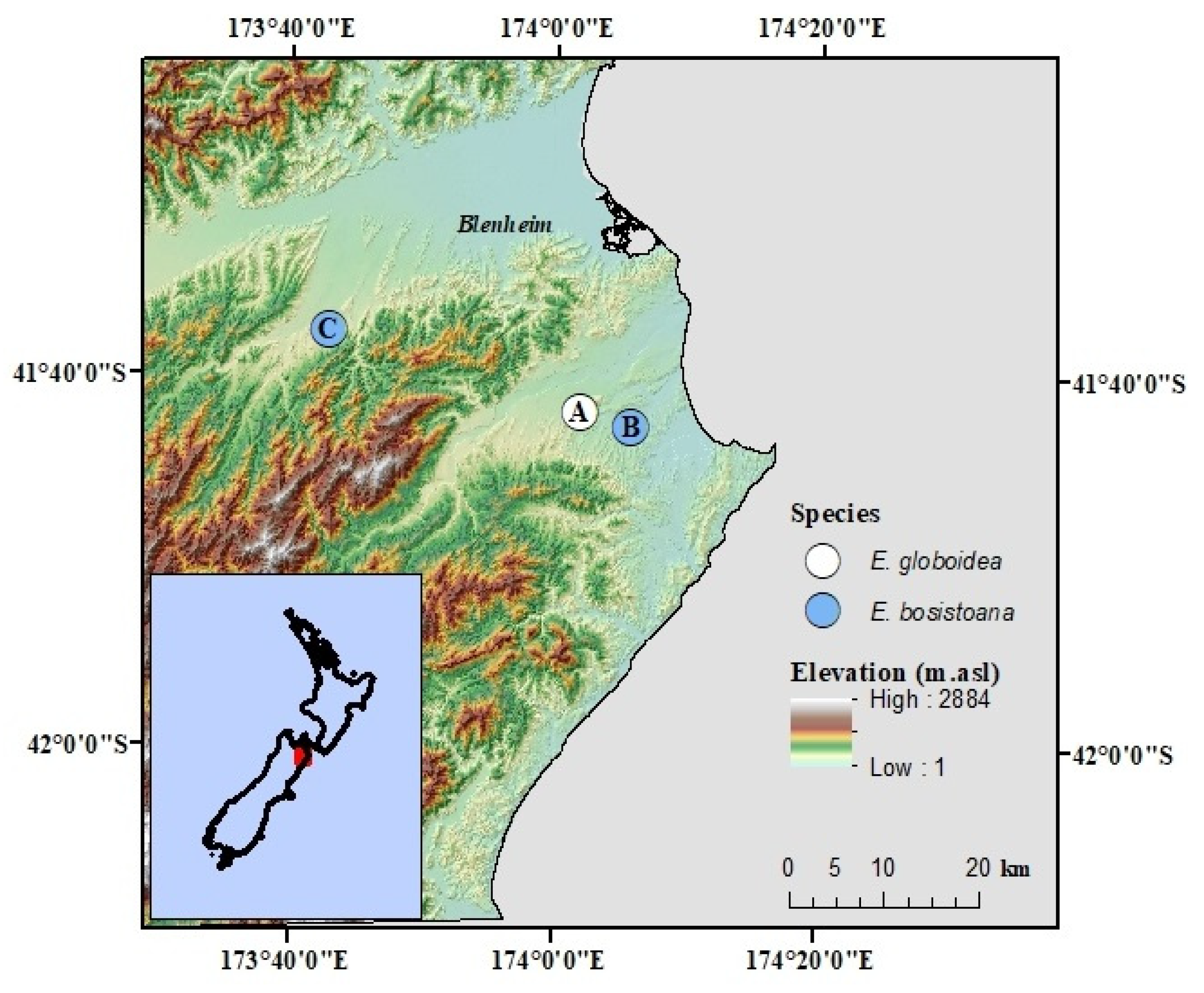
2.1. Experimental Sites

The three experimental sites for this study were chosen based on (i) their locations, (ii) ease of access for carrying instruments and (iii) landowners’ willingness to host the trials. The study sites were situated in a sub-humid zone close to Blenheim, New Zealand (Figure 1). Sites A, B and C, so named to maintain landowner privacy, have areas 4.7, 3.7 and 2.2 hectares, respectively, and are planted with E. globoidea (Site A) and E. bosistoana (Sites B and C) (

Table 1. Summary of the experimental site inventory data.

Site	A				B				C
Est. (Year)	2011				2009				2012
Area (ha)	4.7				3.7				2.2
Trees/ha	2243				1460				1767
Age (year)	6				8				5
Variable	Height		Survival		Height		Survival		Height		Survival
	Fitting	Validation	Fitting	Validation	Fitting	Validation	Fitting	Validation	Fitting	Validation	Fitting	Validation
Plots (n)	217	65	217	65	112	38	-	-	81	27	81	27
Mean	1.54	1.48	0.75	0.74	4.88	4.99	-	-	2.11	2.04	0.99	0.99
Min	0.33	0.46	0.19	0.33	0.98	1.07	-	-	1.29	1.26	0.89	0.92
Max	4.58	3.67	1.00	1.00	13.47	13.66	-	-	3.74	2.93	1.00	1.00
SD	0.84	0.73	0.18	0.19	2.60	2.69	-	-	0.52	0.44	0.02	0.02

).

The region in which the trial sites are located is sheltered by high country to the west, south and in some areas to the east, and it is one of the sunniest regions of New Zealand with 2487 mean annual hours of sunshine [56]. Warm, dry and settled weather predominates during summer, while winter days often begin with a frost, but are usually mild overall. Typical summer daytime maximum air temperatures range from 20 °C to 26 °C but occasionally rise above 30 °C. Typical winter daytime maximum air temperatures range from 10 °C to 15 °C [56]. South-westerly winds prevail in Blenheim, though dry Foehn winds from the northwest also occur [56]. The soils at these sites are formed from loess and classified as Pallic Argillic soils, which have thin subsoil bands of accumulated clay [57] (

Table 2. Soil description of three sites according to Hewitt [58].

Site	Soil Series	Dominant Soil Type	Class Name	Comments
A	Flaxbourne	Hill soils	Typic argillic pallic	Argillic pallic soils have a clay accumulation in the sub-soils
B	Flaxbourne	Hill soils	Typic argillic pallic
C	Wither	Hill soils	Argillic-sodic fragic pallic	Fragic pallic soils are predominantly silty and severely restrict root movement

).

2.2. Data Collection and Preparation

2.2.1. Tree Data

Trees and measurement plots on sites A, B and C were established respectively in 2011, 2009 and 2012. Sites A and C have 282 and 108 plots respectively, with each plot measuring 14.4 m × 10.8m. Site B has 150 plots measuring 12 m × 10.8 m (Table 1). Trees were planted in regular rows and columns within plots, with spacing equal to 2.4 m × 1.8 m in all sites. Weeds were controlled with herbicide in 1 m diameter spots around each tree immediately after establishment.

There were approximately 18,500 trees at the three sites with varying stand density (Table 1). The height (h), diameter at breast height 1.4 m (DBH), and tree status (dead or alive) were measured for all trees. All tree measurements were undertaken during November 2015 and January 2016 and again in June-August 2017 (Table 1). Prior to these measurements, the height and tree status were measured at age 1.2 years for all trees. Individual tree height and survival data were averaged at each plot. The survival proportion (S) was calculated for each plot from the number of surviving trees.

Height data from all three sites were used to create juvenile height models. For survival data, only the A and C sites’ survival proportions (S) were used to create juvenile survival models, as there was a thinning trial at site B prior to completion of field measurements for this study.

2.2.2. Topographic Data

Digital elevation models (DEMs) for all sites were produced by using a real-time kinetic geo-positioning system (RTK-GPS). The unit was carried on transect lines across the sites, with coordinates and elevation collected at five-metre intervals along the transects. The elevation points were interpolated into a DEM with five metre spatial resolution through topo-raster algorithm (ANUDEM), using a process detailed in Salekin, et al. [43].

Next, primary and secondary surface attributes were derived from the DEM for each plot (~15 m spatial resolution). The primary surface attributes included aspect and slope [59]. From these, the following secondary surfaces were derived: Total (CURV), profile (CVPRO) and plan curvature (CVPLA) [60,61]; topographic ruggedness index (TRI) [62]; topographic position index (TPI) [63]; topographic wetness index (TWI) [64,65]; wind exposure index (WEI) [66]; morphometric protection index (MPI) [67] and Euclidian distance between each plot’s centre pixel and the nearest ridge line (DIST) (detailed descriptions of these indices are provided as supplementary material, S1). All surfaces were interpolated or derived using ArcMap 10.4 [68] or the System for Automated Geoscientific Analysis (SAGA) [69]. A summary of the topographic attributes is presented in

Table 3. Summary of the topographic attributes for study sites. TPI—topographic ruggedness index; TRI—topographic position index; TWI—topographic wetness index; WEI—wind exposure index; MPI—morphometric protection index; DIST—Euclidian distance between each plot’s centre pixel and the nearest ridge line.

Attributes	Site A				Site B				Site C
	Min	Max	Mean	SD	Min	Max	Mean	SD	Min	Max	Mean	SD
Aspect (°)	4.57	356.20	127.01	136.8	55.7	345.9	124.5	83.6	208.7	330.1	265.7	26.44
Slope (°)	13.9	31.70	24.60	3.54	11.95	30.37	21.35	3.22	8.56	29.38	21.70	4.56
Elevation (m asl)	13.4	79.22	44.87	16.93	134	168.1	148.7	9.62	232.9	277.5	257.2	12.38
Total curvature	−2.40	3.81	0.11	1.15	−1.83	4.93	0.20	1.17	−3.34	2.78	0.30	1.31
Prof. curvature	−2.79	1.82	−0.01	0.69	−2.21	1.30	−0.11	0.62	−1.79	3.12	0.00	0.86
Plan curvature	−1.83	2.32	0.10	0.79	−1.27	2.73	0.09	0.75	−1.76	2.40	0.30	0.76
TRI	0.47	1.24	0.92	0.15	0.07	0.22	0.14	0.02	0.05	0.18	0.13	0.03
TPI	−2.25	3.52	0.12	0.96	−13.80	13.12	−0.81	7.30	−14.4	10.42	−1.44	6.92
TWI	0	3.90	0.89	0.68	−0.05	2.83	0.89	0.52	0	6.91	3.45	3.70
WEI	0.98	1.10	1.02	0.02	0.88	1.20	0.99	0.08	0.96	1.10	1.03	0.03
MPI	0.07	0.19	0.14	0.02	0.06	0.18	0.12	0.02	0.05	0.18	0.13	0.03
DIST (m)	0.38	140.58	65.40	33.22	1.64	103.55	44.76	25.53	7.58	80.98	36.93	18.64

.

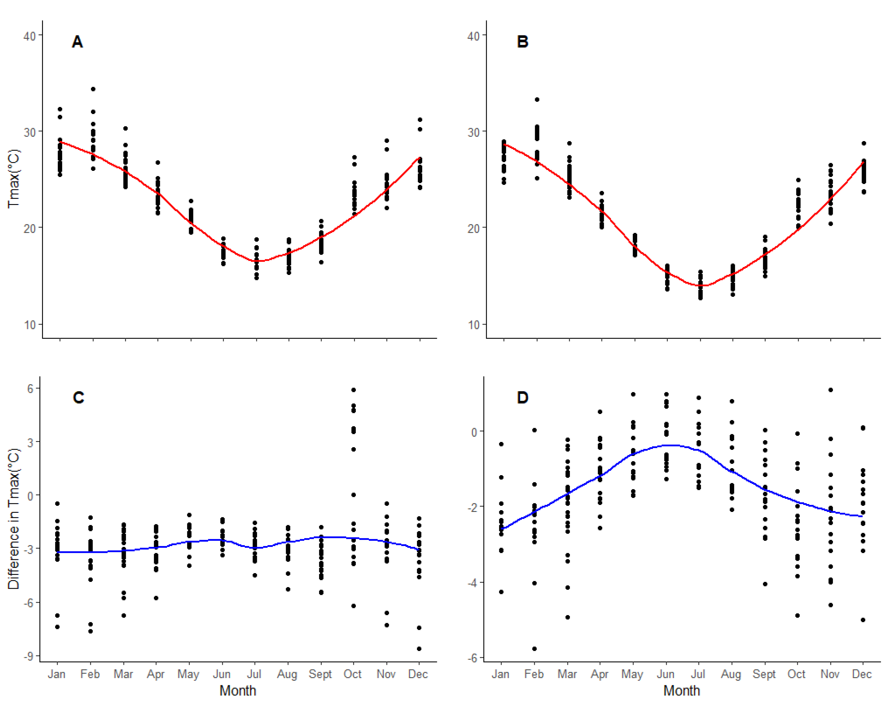
2.2.3. Climatic Data

Each site had a meteorological station, which was equipped with solar radiation, air temperature, soil moisture, wind and rain sensors. There were 20 additional air temperature sensors installed at sites A (n = 10) and B (n = 10), one meter above ground to measure the air temperature variation across and within the sites. All the sensors, including those within the meteorological stations, logged data at 30-minute intervals from March 2015 to April 2017.

Average and maximum daily air temperatures were calculated on a monthly basis for the duration of the measurement period. These calculations were based on data collected by the 10 sensors at each of sites A and B (Figure 2). Air temperature differences between these sensors and the single air temperature sensor within each meteorological station were calculated (Figure 2C,D). This was done by deducting the independent sensors’ temperatures from the meteorological station’s above-ground temperature reading. From the calculated air temperature difference and sensors’ positions, a mixed-effect model was developed by linking primary topographic attributes. This model was used to simulate air temperature differences and estimate the air temperature within each microsite. Detail model development procedures and final models are described in supplementary material, S2.

2.3. Modelling Strategy

In young plantations, prior to canopy closure, growth is modelled exponentially, with larger trees having greater leaf and root surface areas than smaller trees. For the measured height for Pinus radiata seedlings planted in plantations in New Zealand Mason and Whyte [32] expressed this growth function as,

$${\overline{\mathrm{h}}}_{\mathrm{T}}={\overline{\mathrm{h}}}_0+{\mathsf{\alpha }\mathrm{T}}^{\mathsf{\beta }}$$

(1)

Here, ${\overline{\mathrm{h}}}_0$ = mean height immediately after planting (in this case, 0.25 m), and ${\overline{h}}_T$ = mean height at stand age T.

Equation (1) has been widely used for modelling juvenile crops [32,70]. Furthermore, Mason and Whyte [32] showed that the coefficients of Equation (1) could be extended as a linear function (Equations (2) and (3)) to independent variables and their interactions by inserting them into linear functions.

$$\mathsf{\alpha }={\mathsf{\alpha }}_0+{\mathsf{\alpha }}_1{\mathrm{V}}_1+\cdots +{\mathsf{\alpha }}_{\mathrm{n}}{\mathrm{V}}_{\mathrm{n}}$$

(2)

$$\mathsf{\beta }={\mathsf{\beta }}_0+{\mathsf{\beta }}_1{\mathrm{V}}_1+\cdots +{\mathsf{\beta }}_{\mathrm{n}}{\mathrm{V}}_{\mathrm{n}}$$

(3)

The mortality of trees in young plantations is not due to competition among them, but rather water stress or other site-specific factors. According to Mason and Whyte [32] juvenile mortality should be considered as a random process over time with as varying parameter and, therefore, should follow a Weibull probability distribution. The functional form should be anamorphic, as the percentage of deaths would be independent of stocking.

The survival function used by Belli and Ek [70] was one of exponential decay, which was converted to mortality by taking the same Weibull probability density function derivatives given by Mason [71]. Other modellers have used similar approaches [25,70,72]. In this case, the survival proportion function fitted a yield form described in Mason and Whyte [32] (Equation (4)).

$${\mathrm{S}}_{\mathrm{T}}=-{\mathrm{e}}^{\mathsf{\alpha }{\mathrm{T}}^{\mathsf{\beta }}}$$

(4)

where, ${\mathrm{S}}_{\mathrm{T}}$ = survival at stand age T, and α and β represent model coefficients.

It is expected that the coefficients should vary with independent explanatory variables, which can be extended linearly by following the same approach as for the height models (Equations (2) and (3)).

2.4. Model Testing and Validation

A mixed approach [73,74] was applied to evaluate the model, by performing a full set of residual analyses. Validation included a visual analysis of graphs of the residuals, the calculation of standard error (SE) (Equation (5)), root mean square error (RMSE) (Equation (6)), mean absolute error (MAE) (Equation (7)), and bias (Equation (8)).

$$\mathrm{SE}=\frac{\mathrm{S}}{\sqrt{\mathrm{N}}}$$

(5)

$$\mathrm{RMSE}=\sqrt{\frac{{{\displaystyle \sum }}_{\mathrm{i}=1}^{\mathrm{N}}{({\mathrm{P}}_{\mathrm{i}}-{\mathrm{O}}_{\mathrm{i}})}^2}{\mathrm{N}}}$$

(6)

$$\mathrm{MAE}=\frac{{{\displaystyle \sum }}_{\mathrm{i}=1}^{\mathrm{N}}|{\mathrm{P}}_{\mathrm{i}}-{\mathrm{O}}_{\mathrm{i}}|}{\mathrm{N}}$$

(7)

$$\mathrm{bias}=\frac{{{\displaystyle \sum }}_{\mathrm{i}=1}^{\mathrm{N}}({\mathrm{P}}_{\mathrm{i}}-{\mathrm{O}}_{\mathrm{i}})}{\mathrm{N}}$$

(8)

where $\mathrm{S}$= standard deviation of the mean, N = number of observations, $\mathrm{O}$ = observed value, $\mathrm{P}$ = predicted value.

There are many established procedures to perform model validation [75]. Should independent datasets not be available, splitting data sets is a commonly accepted practice for model testing and validation, assuming the dataset is sufficiently large [73]. Dobbin, et al. [76] suggested a data splitting ratio of 75:25 (model fitting: validation), which was applied in this study.

2.5. Statistical Analysis

All statistical analyses were performed in the R statistical environment [77]. An assessment for multi-collinearity was performed for all explanatory variables by using the variation inflation factor (VIF) with the “vif.mer” function of the car package in R [78]. Elevation, slope, topographic ruggedness index (TRI), and total curvature were highly correlated with other potential independent variables. So by following Cook, et al. [79], the R procedure “anova” for comparing models was employed to determine whether or not these variables added any statistically significant extra information and they were excluded from the model building procedure. Following multi-collinearity analysis, model coefficients were fitted against the explanatory variables by using the “lm” function to predict α and β coefficients for Equations (1) and (4) fitted to data from individual plots.

Finally, height and survival models were fitted using the “nls” function with only significant independent variables. The height and survival models were validated against the validation datasets by using “rmse”,”mae” and “bias” functions from the metrics and qpcR packages [80,81].

3. Results

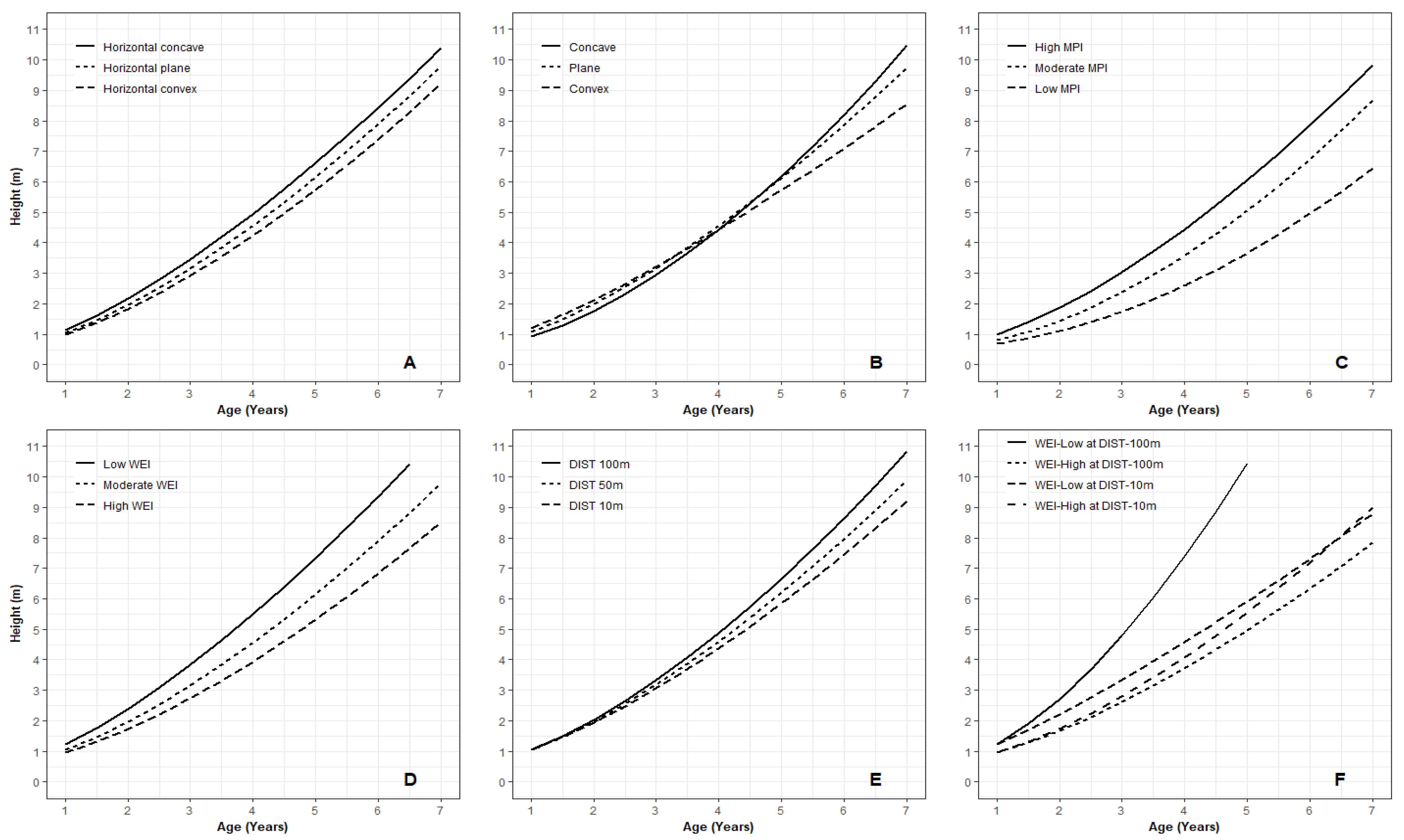
3.1. Juvenile Height Models

Juvenile height models for both species (Equations (9)–(11)) had low and stable error statistics (

Table 4. Fit and validation statistics for the final height growth equations.

Species	Site	Action	RMSE	MAE	BIAS	SE
E. globoidea	A	Fitting	0.453	0.338	0.009	0.435
		Validation	0.348	0.273	0.011	0.350
E. bosistoana	B	Fitting	0.518	0.385	0.032	0.521
		Validation	0.603	0.429	0.024	0.614
	C	Fitting	0.342	0.274	0.001	0.347
		Validation	0.322	0.251	0.001	0.339

). The residuals of the models satisfied all required statistical assumptions (Supplementary material, S3), they were normally distributed and had minimum bias and heteroscedasticity. The E. globoidea model over-predicted height. With the exception of bias, all calculated statistics were lower for the fitting dataset than for the validation dataset (see Table 4).

$${\mathrm{h}}_{{\mathrm{EGT}}_{\mathrm{A}}}={\mathrm{h}}_{\mathrm{EG}0}+\left({\mathsf{\alpha }}_0+{\mathsf{\alpha }}_1\ast \mathrm{WEI}+{\mathsf{\alpha }}_2\ast \mathrm{DIST}\right)\ast {\mathrm{T}}_{\mathrm{EGT}}{}^{\left({\mathsf{\beta }}_0+{\mathsf{\beta }}_1\ast \mathrm{DIST}+{\mathsf{\beta }}_2\ast \mathrm{WEI}+{\mathsf{\beta }}_3\ast \mathrm{MPI}\right)}$$

(9)

$$\begin{array}{cc}\hfill {\mathrm{h}}_{{\mathrm{EBT}}_{\mathrm{B}}}={\mathrm{h}}_{\mathrm{EB}0}+& \left({\mathsf{\alpha }}_0+{\mathsf{\alpha }}_1\ast \mathrm{CVPLA}+{\mathsf{\alpha }}_2\ast \mathrm{TPI}+{\mathsf{\alpha }}_3\ast \mathrm{WEI}+{\mathsf{\alpha }}_4\ast \mathrm{MPI}\right)\hfill \\ & \ast {\mathrm{T}}_{\mathrm{EBT}}{}^{\left({\mathsf{\beta }}_0+{\mathsf{\beta }}_1\ast \mathrm{CVPLA}+{\mathsf{\beta }}_2\ast \mathrm{WEI}+{\mathsf{\beta }}_3\ast \mathrm{MPI}+{\mathsf{\beta }}_4\ast \mathrm{TPI}+{\mathsf{\beta }}_5\ast \mathrm{DIST}+{\mathsf{\beta }}_6\ast \mathrm{WEI}:\mathrm{DIST}\right)}\hfill \end{array}$$

(10)

$$\begin{array}{c}{\mathrm{h}}_{{\mathrm{EBT}}_{\mathrm{c}}}={\mathrm{h}}_{\mathrm{EB}0}+\left({\mathsf{\alpha }}_0+{\mathsf{\alpha }}_1\ast \mathrm{WEI}+{\mathsf{\alpha }}_2\ast \mathrm{TWI}+{\mathsf{\alpha }}_3\ast \mathrm{TPI}+{\mathsf{\alpha }}_4\ast \mathrm{MPI}+{\mathsf{\alpha }}_5\ast \mathrm{DIST}\right)\ast \\ {\mathrm{T}}_{\mathrm{EBT}}{}^{\left({\mathsf{\beta }}_0+{\mathsf{\beta }}_1\ast \mathrm{TPI}+{\mathsf{\beta }}_2\ast \mathrm{DIST}\right)}\end{array}$$

(11)

where ${\mathrm{h}}_{{\mathrm{EGT}}_{\mathrm{A}}}$ is the E. globoidea height at time T in site A; ${\mathrm{h}}_{{\mathrm{EBT}}_{\mathrm{B}}}$ and ${\mathrm{h}}_{{\mathrm{EBT}}_{\mathrm{c}}}$ are the E. bosistoana height at time T respectively in sites B and C. ${\mathrm{h}}_{\mathrm{EG}0}$ and ${\mathrm{h}}_{\mathrm{EB}0}$ are the initial height of E. globoidea and E. bosistoana. ${\mathrm{T}}_{\mathrm{EGT}}$ and ${\mathrm{T}}_{\mathrm{EBT}}$ are the age of E. globoidea and E. bosistoana. Other terms have previously been defined. Model parameters are provided in Supplementary material 5 (Table I).

The E. bosistoana height model behaved differently at different sites. At site B, the model standard error was higher than that of site C (Table 4). At site B, RMSE, MAE and SE increased respectively to 0.603, 0.429 and 0.615 from the fit statistics, while BIAS reversed in turn to 0.024 from the fit statistics. In contrast to that, at site C all the fitting statistics features were reduced during validation (Table 4).

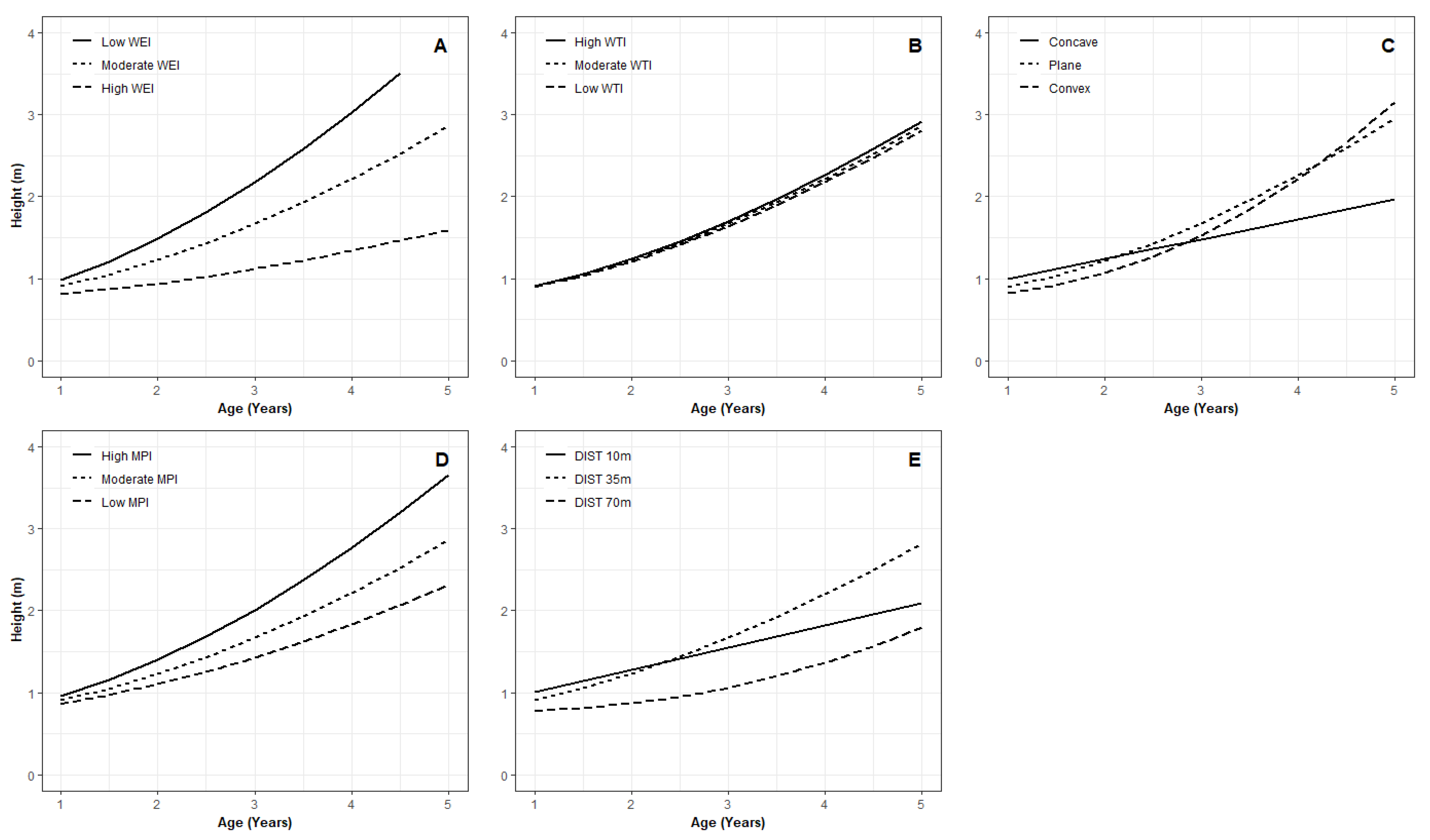
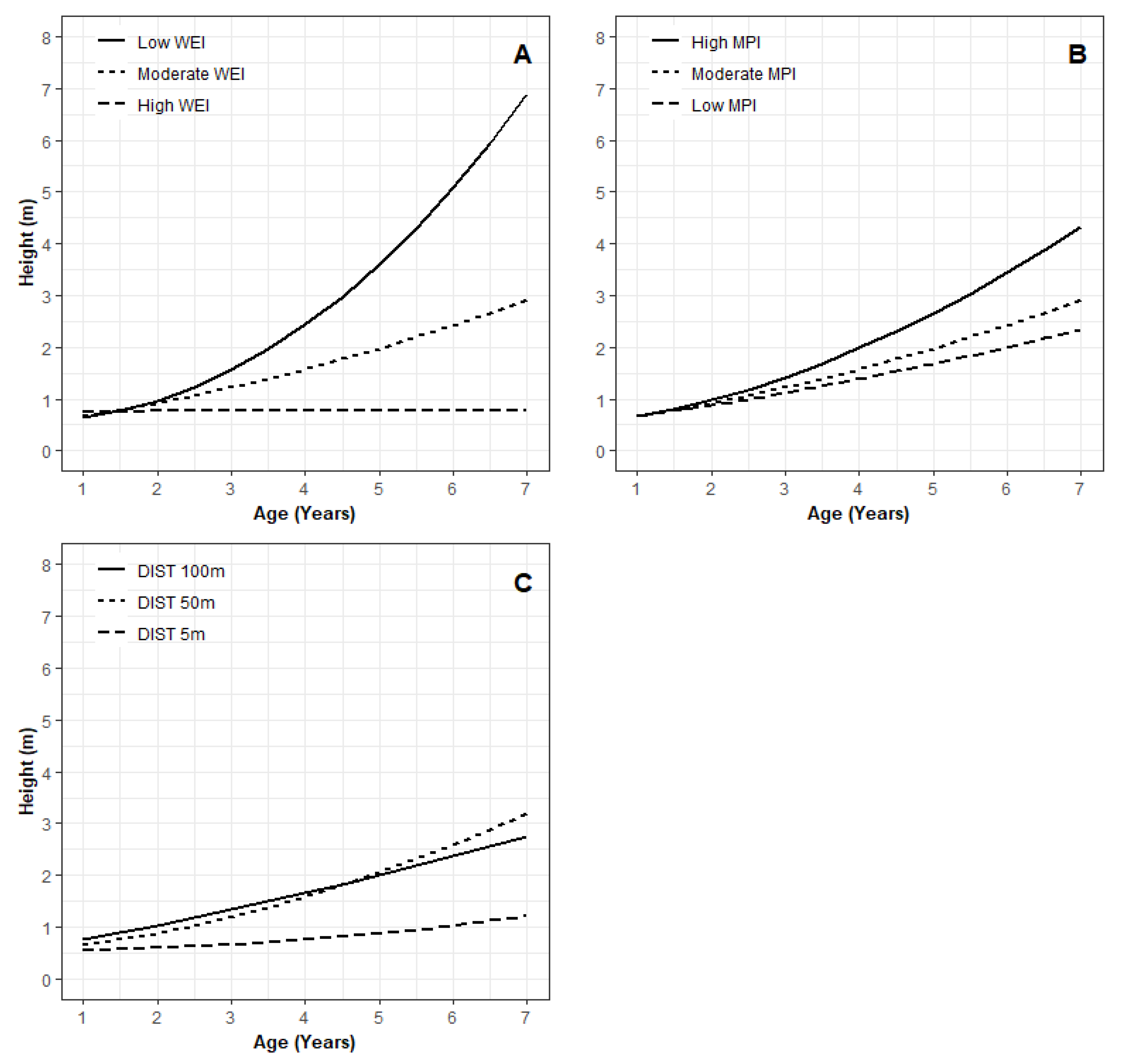
3.2. Key Variables for Microsite Height Growth

Juvenile E. globoidea height at Site A was significantly correlated with WEI, MPI and plot distance from the top ridge (DIST) (

Table 5. Tested variables and their significance on juvenile height growth at the three sites.

Variables	p-Values at Different Sites
	A	B	C
Maximum daily temperature	NS	NS	NS
Prof. curvature	NS	NS	NS
Plan curvature	NS	0.0001**	NS
TPI	NS	2.72e−08***	0.0020**
WEI	0.0033**	0.0002	0.0010**
TWI	NS	NS	0.0184*
MPI	0.0008***	<2e−16***	7.43e−05***
Distance from the top ridge (DIST)	<2e−16***	<2e−16***	2.22e−05***

Signif. Codes: *** = p < 0.001, ** = p < 0.01; *= p <0.05; NS = p ≥ 0.05.

and Figure 3). Therefore, these variables were added to the final height growth model represented by Equation (9). The microsites exposed to high levels of wind had the least height growth, and tree height growth decreased with reduced morphometric protection (MPI). Trees close to the top ridge had the least height growth, while height growth increased proportionally with distance from the ridge until the age of 4.5 years. Beyond that age, trees at the mid-distance from the top ridge grew taller.

Eucalyptus bosistoana height growth was influenced by different factors at different sites (Table 5). At site B, CVPLA, MPI, DIST, TPI, WEI and the interaction between WEI and DIST influenced tree height (Figure 4). In sites with local horizontal concave surfaces, trees were taller than the trees on horizontal flat or convex surfaces. TPI also showed a similar pattern, whereby trees were taller in valleys than on ridges. Until age 4.5 years, trees nearer the top ridge experienced faster height growth than trees further from the top ridge, but after that age, the converse was true (Figure 4D). MPI and WEI were correlated positively and negatively, respectively, with height growth, suggesting that exposure to wind and other environmental stresses may have suppressed height growth. However, the lowest WEI with distant microsite had the highest height growth compare to low WEI and a position close to the ridge. On the other hand, high WEI with the farthest microsite, which means close to the valley floor, was the worst for tree height at the B site.

In the case of site C, E. bosistoana height was affected by WEI, WTI, TPI, MPI and DIST (Figure 5). The MPI and WEI effects were similar to other results, with high MPI and low WEI resulting in increased tree height (Figure 5A and 5E). An increase of TPI affected the tree height up to age 2.5 years, after which the effect was reversed, such that trees in valleys had greater height growth, relative to trees on mid-slopes or ridges. The trees situated at mid-distance from the ridge top grew taller than those closest to, and furthest from, the ridge top. Interestingly, the surface wetness (TWI) minimally influenced tree height (Figure 5B).

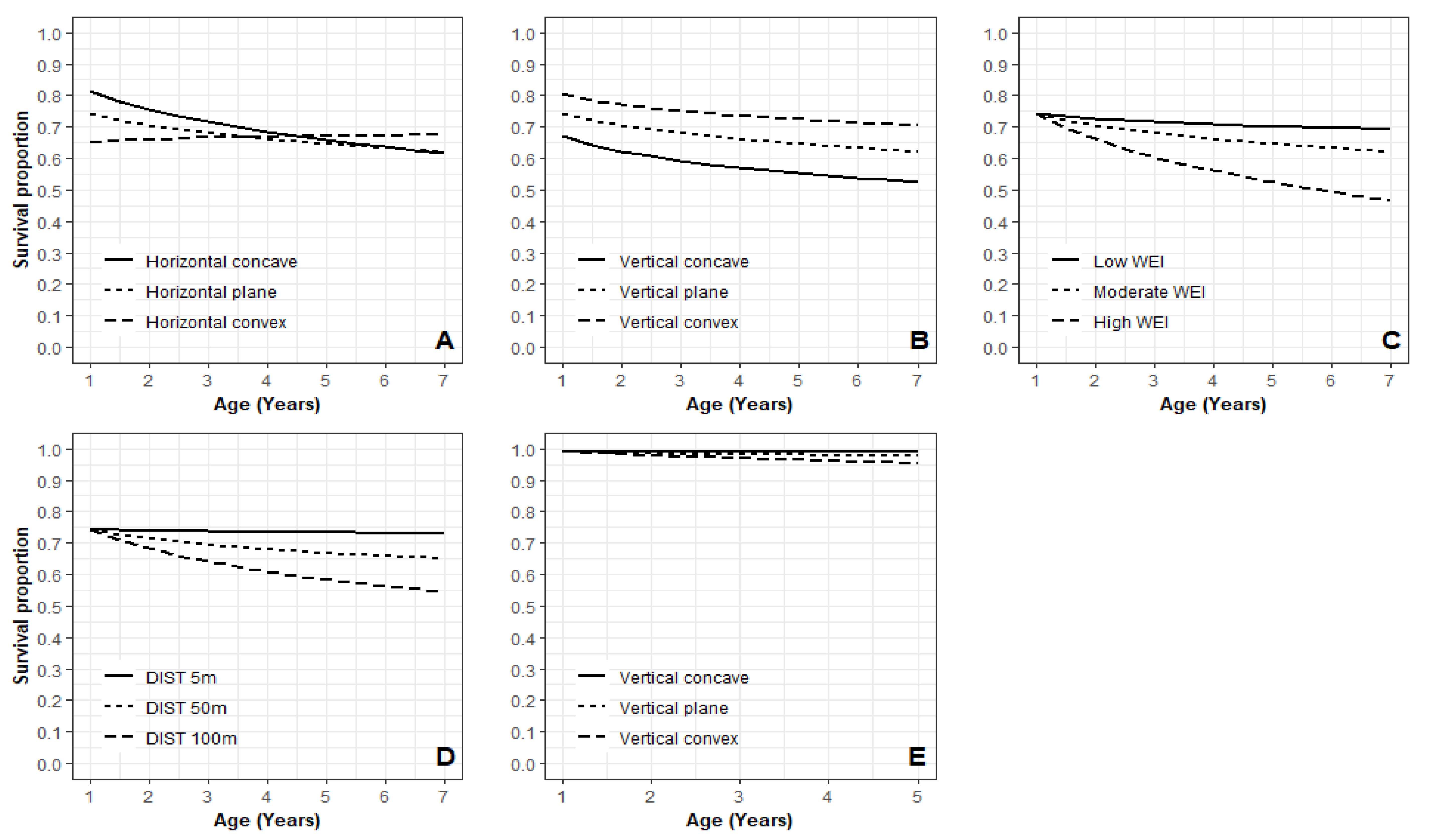
3.3. Juvenile Survival Model

Analyses revealed that the smallest residual mean squares and the least biased residuals were produced by augmenting survival models (Equations (12) and (13)) with topographic attributes. The rate of mortality diminished with time in most plots, but mortality was greater in later years than in early years.

$${\mathrm{S}}_{{\mathrm{EGT}}_{\mathrm{A}}}=-{\mathrm{e}}^{\left({\mathsf{\alpha }}_0+{\mathsf{\alpha }}_1\ast \mathrm{CVPLA}+{\mathsf{\alpha }}_2\ast \mathrm{CVPRO}\right)\ast {\mathrm{T}}^{\left({\mathsf{\beta }}_0+{\mathsf{\beta }}_1\ast \mathrm{WEI}+{\mathsf{\beta }}_2\ast \mathrm{DIST}+{\mathsf{\beta }}_3\ast \mathrm{CVPLA}\right)}}$$

(12)

$${\mathrm{S}}_{{\mathrm{EBT}}_{\mathrm{C}}}=-{\mathrm{e}}^{{\mathsf{\alpha }}_0\ast {\mathrm{T}}^{\left({\mathsf{\beta }}_0+{\mathsf{\beta }}_1\ast \mathrm{CVPRO}\right)}}$$

(13)

where, ${\mathrm{S}}_{{\mathrm{EGT}}_{\mathrm{A}}}$ and ${\mathrm{S}}_{{\mathrm{EBT}}_{\mathrm{C}}}$ are the survival proportion of E.globoidea and E. bosistoana at time T in site A and C; other terms have been defined earlier. Model parameters are provided in the supplementary material 5 (Table II).

The residual distribution against predicted and independent datasets was normally distributed with minor distortions for all species and sites (Supplementary material, S3). Validation for both species was undertaken, and the survival proportion model had minimal differences in precision and bias between fitting and validation datasets (

Table 6. Juvenile survival model fitting statistics.

Species	Site	Action	RMSE	MAE	BIAS	SE
E. globoidea	A	Fitting	0.108	0.076	−0.001	0.109
		Validation	0.097	0.068	−2.086e−06	0.099
E. bosistoana	C	Fitting	0.019	0.013	−7.951e−06	0.020
		Validation	0.021	0.015	2.980e−05	0.022

). In the case of E. globoidea, the RMSE and MAE reduced during validation while they increased slightly with E. bosistoana model validation.

3.4. Key Variables Influencing Juvenile Microsite Survival

Eucalyptus globoidea survival was influenced by plan and profile curvature, WEI and distance from the ridge top (

Table 7. Tested variables and their significance on juvenile survival.

Variables	p-Values at Different Sites
	A	C
Maximum daily temperature	NS	NS
Prof. curvature	0.0004***	0.0272*
Plan curvature	0.0387*	NS
TPI	NS	NS
WEI	4.68e−09***	NS
TWI	NS	NS
MPI	NS	NS
DIST	6.81e−09***	NS

Signif. Codes: *** = p < 0.001, ** = p < 0.01; *= p < 0.05; NS = p ≥ 0.05

and Figure 6). In concave and flat areas, mortality rate was steady whereas in convex areas mortality declined with time. This result was repeated for profile curvature, where on the raised surfaces trees survived in higher proportions than on hollow or flat surfaces. Survival decreased with increasing exposure to wind. Moreover, plots a long distance from the ridge top showed lower survival rates than those close to it.

Eucalyptus bosistoana survival was influenced only by profile curvature (Figure 6E). It showed that, in gullies, higher proportions of trees survived than on flat surfaces or ridges.

4. Discussion

4.1. Juvenile Microsite Models

While earlier work has modelled juvenile trees on a broad scale (e.g., [30,32]), the juvenile microsite models described here have shown the utility of modelling juvenile crops at a finer scale. Individual juvenile trees have also been modelled by applying mathematical equations [25,82,83] and explaining different competing variables [82,84,85]. Kohama, et al. [86] and Weiskittel, et al. [21] studied juvenile and mature stand tree growth on a micro-scale, and Weiskittel, et al. [21] proposed a modelling framework but only for mature stand trees. However, juvenile and mature trees have different growth requirements and competition indices. The models presented in this study for juvenile trees have field applicability, which could be incorporated into a decision support system for silviculture at sites with similar characteristics, because previous research has shown that factors affecting juvenile crop growth and survival can have rotation-length implications [31,87,88].

4.2. Microsite Variables Affect Juvenile Tree Height Growth

This study showed that juvenile tree height growth and survival were affected by microsite- related variables. Millner and Kemp [55] found similar results with other Eucalyptus species in Tuapaka, New Zealand. Topographic variables are major drivers of tree growth in many hilly regions [55,89], as they relate to both climatic and edaphic factors [90]. Height growth of both species in this study was greater in more sheltered microsites. Similar results were found by Brüchert, et al. [91] who showed that wind could influence the aerial architecture of the trees.

Generally, valley floors can be expected to have greater rooting depth [92] and less direct solar radiation as well as radiative heat [93], meaning that trees are better physiologically supported in terms of nutrients and moisture. However, this study found that mid-slopes, measured as distance from the ridge top, were best for E. globoidea. This may be due to mid-slopes provided optimum soil moisture availability to this species and it may be sensitive to the assumed elevated soil moisture and associated anaerobic soil conditions commonly found at valley floors [92,94].

Eucalyptus bosistoana grew taller in concave, depressed (valley) surfaces, and in locations farthest from ridges, which had relatively low wind exposure index. This can be explained in a similar way to E. globoidea but suggests that this species may be more water-demanding, or alternatively, tolerant of soil wetness than E. globoidea at young ages. Rohner, et al. [95] and Monserud, et al. [96] reported that the steep slopes resulted in shallow soil and less moisture availability due to lateral moisture flow. This is in line with the topographic position index effect, as it described each microsite with respect to slope.

4.3. Microsite Variability on Juvenile Tree Survival

Eucalyptus globoidea was apparently sensitive to assumed higher soil moisture levels and reduced growth, but the species could withstand drier conditions. Conversely, E. bosistoana showed less sensitivity to assumed higher moisture levels compared with E. globoidea. This suggested that E. globoidea may experience above-optimal levels of soil moisture (possibly due to anaerobic soil conditions) for tree survival, in both valleys and hollows. Conversely, E. bosistoana survived better in gullies, where there is presumably a chance to access higher moisture availability. Moreover, Ares and Marlats [89] found and concluded that in mountain regions of Argentina coniferous trees died on north-facing slopes, as this aspect receives more radiative heat than other aspects, which may increase water stress. Mason and Whyte [32] reported that frost negatively influenced juvenile tree survival, which could be an alternative or additional reason for increased mortality of E. globoidea in hollows.

4.4. Data Constraints

The initial height for the young Eucalyptus plantations was not recorded immediately after planting. For that reason, the initial height model was fitted by assuming Eucalyptus seedlings met New Zealand’s Pinus radiata (D. Don) plantation standard, which was 0.25 m in height at time of planting [32]. The use of this standard height value might have influenced model stability at the early ages because the model extrapolated the height values for that age. Therefore, these models should be used cautiously over the period from planting to first measurement age. The genetics of each species may be a factor in the response to the environmental conditions. Gallart, et al. [23] showed that some P. radiata genotypes were more sensitive to microsite changes in soil physical properties than other, the same seed sources for both species were used across all three sites. Also, the design of these experiments was not orthogonal. Therefore, it is likely that there was some spatial autocorrelation between each replicate which may have influenced final results.

High resolution soil information describing physical and chemical characteristics were not available for these sites. Since the plantations were not established on sites with homogeneous soil conditions, this may be a confounding factor. High resolution soil data may have improved model precision and explanatory ability. Future studies should consider including fine-scale soil data, and plan accordingly for the associated time and financial costs.

Likewise, including fine-scale climatic variables into the models may have given greater explanatory power and understanding of causal processes [97,98]. However, in this study, only air temperature was considered but not selected for inclusion in the final model as it was not statistically significant. Solar radiation, wind speed, soil moisture and precipitation were not considered because data were not available at a sufficiently fine resolution as each site had only one meteorological station.

5. Summary and Conclusions

This study successfully demonstrated a statistically and biologically logical framework for modelling juvenile tree growth and survival at a microsite level. It also identified and explained height and survival variation of two Eucalyptus species at high spatial resolution on three sites. For both species, topographically sheltered surfaces yielded greater height growth and survival. Furthermore, there were different microsite factors that each species required for optimal growth and survival. The topographic features in this study indicated that soil moisture could be an important factor in explaining height growth and survival, with E. globoidea being negatively affected in valleys and hollows, where available moisture is presumably high. Conversely, E. bosistoana thrived in these environments. More research is required for these valuable Eucalyptus species over a larger environmental gradient of potential afforestation sites to understand the full suite of microsite factors and their interactions. However, the results of this study provide important information that will assist forest managers to identify sites and microsites where it is best to establish each species.

The study indicates that researchers wishing to evaluate effects of microsite variation on tree crop growth are likely to find high resolution digital elevation models more useful than randomly allocated soil pits and sparse soil analyses. Indices of land form variation derived from the digital elevation model were surprisingly well correlated with tree crop performance.

References

1. Radford, I.J.; Nicholas, M.; Tiver, F.; Brown, J.; Kriticos, D. Seedling establishment, mortality, tree growth rates and vigour of Acacia nilotica in different astrebla grassland habitats: Implications for invasion. Austral Ecol. 2002, 27, 258–268. [Google Scholar] [CrossRef]
2. Bailey, R.G.; Pfister, R.D.; Henderson, J.A. Nature of land and resource classification—A review. J. For. 1978, 76, 650–655. [Google Scholar]
3. Grey, D. On the concept of site in forestry. S. Afr. For. J. 1980, 113, 81–83. [Google Scholar] [CrossRef]
4. Louw, J.H. A review of site-growth studies in south africa. S. Afr. For. J. 1999, 185, 57–65. [Google Scholar] [CrossRef]
5. Skovsgaard, J.P.; Vanclay, J.K. Forest site productivity: A review of the evolution of dendrometric concepts for even-aged stands. Forestry 2008, 81, 13–31. [Google Scholar] [CrossRef]
6. Skovsgaard, J.P.; Vanclay, J.K. Forest site productivity: A review of spatial and temporal variability in natural site conditions. Forestry 2013, 86, 305–315. [Google Scholar] [CrossRef]
7. Dungey, H.S.; Dash, J.P.; Pont, D.; Clinton, P.W.; Watt, M.S.; Telfer, E.J. Phenotyping whole forests will help to track genetic performance. Trends Plant Sci. 2018, 23, 854–864. [Google Scholar] [CrossRef]
8. Koch, G.W.; Sillett, S.C.; Jennings, G.M.; Davis, S.D. The limits to tree height. Nature 2004, 428, 851–854. [Google Scholar] [CrossRef]
9. Forrester, D.I. Linking forest growth with stand structure: Tree size inequality, tree growth or resource partitioning and the asymmetry of competition. For. Ecol. Manag. 2019, 447, 139–157. [Google Scholar] [CrossRef]
10. Berrill, J.P.; O’Hara, K.L. How do biophysical factors contribute to height and basal area development in a mixed multiaged coast redwood stand? Forestry 2016, 89, 170–181. [Google Scholar] [CrossRef]
11. Bravo-Oviedo, A.; Tomé, M.; Bravo, F.; Montero, G.; del Río, M. Dominant height growth equations including site attributes in the generalized algebraic difference approach. Can. J. For. Res. 2008, 38, 2348–2358. [Google Scholar] [CrossRef]
12. Landsberg, J. Physiology in forest models: History and the future. FBMIS 2003, 1, 49–63. [Google Scholar]
13. Wiens, J.A. Spatial scaling in ecology. Funct. Ecol. 1989, 3, 385–397. [Google Scholar] [CrossRef]
14. Chen, J.; Saunders, S.C.; Crow, T.R.; Naiman, R.J.; Brosofske, K.D.; Mroz, G.D.; Brookshire, B.L.; Franklin, J.F. Microclimate in forest ecosystem and landscape ecology variations in local climate can be used to monitor and compare the effects of different management regimes. BioScience 1999, 49, 288–297. [Google Scholar] [CrossRef]
15. Lilja-Rothsten, S.; Chantal, M.D.; Peterson, C.; Kuuluvainen, T.; Vanha-Majamaa, I.; Puttonen, P. Microsites before and after restoration in managed Picea abies stands in southern finland: Effects of fire and partial cutting with dead wood creation. Silva Fenn. 2008, 42, 165–176. [Google Scholar] [CrossRef]
16. Coates, K.D. Tree recruitment in gaps of various size, clearcuts and undisturbed mixed forest of interior British Columbia, Canada. For. Ecol. Manag. 2002, 155, 387–398. [Google Scholar] [CrossRef]
17. Kuuluvainen, T. Natural variability of forests as a reference for restoring and managing biological diversity in boreal fennoscandia. Silva Fenn. 2002, 36, 97–125. [Google Scholar] [CrossRef]
18. Martín-Alcón, S.; Coll, L.; Salekin, S. Stand-level drivers of tree-species diversification in mediterranean pine forests after abandonment of traditional practices. For. Ecol. Manag. 2015, 353, 107–117. [Google Scholar] [CrossRef]
19. Narukawa, Y.; Yamamoto, S.I. Gap formation, microsite variation and the conifer seedling occurrence in a subalpine old-growth forest, central japan. Ecol. Res. 2001, 16, 617–625. [Google Scholar] [CrossRef]
20. Ahtikoski, A.; Siipilehto, J.; Salminen, H.; Lehtonen, M.; Hynynen, J. Effect of stand structure and number of sample trees on optimal management for scots pine: A model-based study. Forests 2018, 9, 750. [Google Scholar] [CrossRef]
21. Weiskittel, A.; Temesgen, H.; Wilson, D.; Maguire, D. Sources of within- and between-stand variability in specific leaf area of three ecologically distinct conifer species. Ann. For. Sci. 2008, 65, 103. [Google Scholar] [CrossRef]
22. Mummery, D.; Battaglia, M. Data input quality and resolution effects on regional and local scale Eucalyptus globulus productivity predictions in north-east tasmania. Ecol. Model. 2002, 156, 13–25. [Google Scholar] [CrossRef]
23. Gallart, M.; Love, J.; Meason, D.F.; Coker, G.; Clinton, P.W.; Xue, J.; Jameson, P.E.; Klápště, J.; Turnbull, M.H. Field-scale variability in site conditions explain phenotypic plasticity in response to nitrogen source in Pinus radiata d. Don. Plant Soil 2019. [Google Scholar] [CrossRef]
24. Spiecker, H.; Mieläikinen, K.; Köhl, M.; Skovsgaard, J.P. Discussion. In Growth Trends in European Forests; Spiecker, H., Mielikäinen, K., Köhl, M., Skovsgaard, J., Eds.; Springer: Berlin/Heidelberg, Germany, 1996; pp. 355–367. [Google Scholar]
25. Zhang, S.; Burkhart, H.E.; Amateis, R.L. Modeling individual tree growth for juvenile loblolly pine plantations. For. Ecol. Manag. 1996, 89, 157–172. [Google Scholar] [CrossRef]
26. Clutter, J.L. Compatible growth and yield models for loblolly pine. For. Sci. 1963, 9, 354–371. [Google Scholar]
27. Garcia, O. New class of growth models for even-aged stands: Pinus radiata in golden downs forest. N. Z. J. For. Sci. 1984, 14, 65–88. [Google Scholar]
28. Burkhart, H.E.; Tomé, M. Modeling Forest Trees and Stands; Springer: Berlin/Heidelberg, Germany, 2012. [Google Scholar]
29. Weiskittel, A.R.; Hann, D.W.; Kershaw, J.A.; Vanclay, J.K. Forest Growth and Yield Modeling; Wiley: Hoboken, NJ, USA, 2011. [Google Scholar]
30. Avila, O.B. Modeling Growth Dynamics of Juvenile Loblolly Pine Plantations; Virginia Polytechnic Institute and State Univeristy: Blacksburg, VA, USA, 1993. [Google Scholar]
31. Mason, E.G.; Whyte, A.G.D.; Woollons, R.C.; Richardson, B. A model of the growth of juvenile Radiata pine in the central north island of New Zealand: Links with older models and rotation-length analyses of the effects of site preparation. For. Ecol. Manag. 1997, 97, 187–195. [Google Scholar] [CrossRef]
32. Mason, E.G.; Whyte, A.G.D. Modelling initial survival and growth of Radiata pine in New Zealand. Acta For. Fenn. 1997, 2, 1–38. [Google Scholar] [CrossRef]
33. Casnati, A.C.R. Hybrid Mensurational-Physiological Models for Pinus Taeda and Eucalyptus Grandis in Uruguay. Ph.D. Thesis, University of Canterbury, Christchurch, New Zealand, 2016. [Google Scholar]
34. Ma, P.; Han, X.H.; Lin, Y.; Moore, J.; Guo, Y.X.; Yue, M. Exploring the relative importance of biotic and abiotic factors that alter the self-thinning rule: Insights from individual-based modelling and machine-learning. Ecol. Model. 2019, 397, 16–24. [Google Scholar] [CrossRef]
35. Mason, E.G. A model of the juvenile growth and survival of Pinus radiata d. Don; adding the effects of initial seedling diameter and plant handling. New For. 2001, 22, 133–158. [Google Scholar] [CrossRef]
36. Woollons, R.C.; Snowdon, P.; Mitchell, N.D. Augmenting empirical stand projection equations with edaphic and climatic variables. For. Ecol. Manag. 1997, 98, 267–275. [Google Scholar] [CrossRef]
37. Snowdon, P.; Jovanovic, T.; Booth, T.H. Incorporation of indices of annual climatic variation into growth models for Pinus radiata. For. Ecol. Manag. 1999, 117, 187–197. [Google Scholar] [CrossRef]
38. Mäkelä, A.; Landsberg, J.; Ek, A.R.; Burk, T.E.; Ter-Mikaelian, M.; Ågren, G.I.; Oliver, C.D.; Puttonen, P. Process-based models for forest ecosystem management: Current state of the art and challenges for practical implementation. Tree Physiol. 2000, 20, 289–298. [Google Scholar] [CrossRef] [PubMed]
39. Watt, M.S.; Kimberley, M.O.; Richardson, B.; Whitehead, D.; Mason, E.G. Testing a juvenile tree growth model sensitive to competition from weeds, using Pinus radiata at two contrasting sites in New Zealand. Can. J. For. Res. 2004, 34, 1985–1992. [Google Scholar] [CrossRef]
40. Dyck, B. Precision forestry—The path to increased profitability. In Proceedings of the 2nd International Precision Forestry Symposium, Seattle, WA, USA, 15–17 June 2003; pp. 3–8. [Google Scholar]
41. Adão, T.; Hruška, J.; Pádua, L.; Bessa, J.; Peres, E.; Morais, R.; Sousa, J. Hyperspectral imaging: A review on uav-based sensors, data processing and applications for agriculture and forestry. Remote Sens. 2017, 9, 1110. [Google Scholar] [CrossRef]
42. Akay, A.E.; Oǧuz, H.; Karas, I.R.; Aruga, K. Using lidar technology in forestry activities. Environ. Monit. Assess. 2009, 151, 117–125. [Google Scholar] [CrossRef] [PubMed]
43. Salekin, S.; Burgess, J.; Morgenroth, J.; Mason, E.; Meason, D. A comparative study of three non-geostatistical methods for optimising digital elevation model interpolation. ISPRS Int. J. Geo Inf. 2018, 7, 300. [Google Scholar] [CrossRef]
44. NZFOA. New Zealand Plantation Forest Industry: Facts and Figures 2016/17; Ministry for Primary Industries: Wellington, New Zealand, 2017.
45. Turner, J.A.; West, G.; Dungey, H.; Wakelin, S.; Maclaren, P.; Adams, T.; Silcock, P.J. Managing New Zealand Planted Forests for Carbon: A Review of Selected Scenarios Identification of Knowledge Gaps; The Ministry of Agriculture Forestry: Wellington, New Zealand, 2008; p. 130.
46. Millen, P.; van Ballekom, S.; Altaner, C.; Apiolaza, L.; Mason, E.; McConnochie, R.; Morgenroth, J.; Murray, T. Durable eucalypt forests–a multi-regional opportunity for investment in New Zealand drylands. N. Z. J. For. 2018, 63, 11–23. [Google Scholar]
47. Liu, C.L.C.; Kuchma, O.; Krutovsky, K.V. Mixed-species versus monocultures in plantation forestry: Development, benefits, ecosystem services and perspectives for the future. Glob. Ecol. Conserv. 2018, 15, e00419. [Google Scholar] [CrossRef]
48. van der Plas, F.; Manning, P.; Allan, E.; Scherer-Lorenzen, M.; Verheyen, K.; Wirth, C.; Zavala, M.A.; Hector, A.; Ampoorter, E.; Baeten, L.; et al. Jack-of-all-trades effects drive biodiversity–ecosystem multifunctionality relationships in european forests. Nat. Commun. 2016, 7, 11109. [Google Scholar] [CrossRef]
49. Menzies, H. Eucalypts show potential. Farm For. Rev. 1995, 33–34. [Google Scholar]
50. Nicholas, I.; Millen, P. Durable Eucalypt Leaflet Series: Eucalyptus Bosistoana; NZDFI, Ed.; NZDFI: Blenheim, New Zealand, 2012. [Google Scholar]
51. Nicholas, I.; Millen, P. Durable Eucalypt Leaflet Series: Eucalyptus Globoidea; NZDFI, Ed.; NZDFI: Blenheim, New Zealand, 2012. [Google Scholar]
52. Kakitani, T. The global timberlization movement and the potential for durable eucalyts: Downstream opportunities. In Durable Eucalypts on Drylands: Protecting and Enhanching Value; Altaner, C.M., Murray, T.J., Morgenroth, J., Eds.; NZDFI, Marlborough Research Centre: Blenheim, New Zealand, 2017. [Google Scholar]
53. Satchell, D.; Turner, J. Solid Timber Recovery and Economics of Short-Rotation Small Diameter Eucalypt Forestry Using Novel Sawmilling Strategy Applied to Eucalyptus Regnans; SCION Report No. FFR-DS028; New Zealand Forest Research Institute Limited: Rotorua, New Zealand, 2010. [Google Scholar]
54. Nicholas, I.D. Best Practice with Farm Forestry Timber Species: No. 2 Eucalypts; Farm Forestry Association: Wellington, New Zealand, 2009. [Google Scholar]
55. Millner, J.P.; Kemp, P.D. Seasonal growth of eucalyptus species in New Zealand hill country. New For. 2012, 43, 31–44. [Google Scholar] [CrossRef]
56. NIWA. Overview of New Zealand Climate. Available online: https://www.niwa.co.nz/education-and-training/schools/resources/climate/overview (accessed on 26 August 2015).
57. New Zealand Department of Scientific and Industrial Research. General survey of the soils of South Island New Zealnd. N. Z. Soil Bur. Bull. 1968. [Google Scholar] [CrossRef]
58. Hewitt, A.E. New Zealand Soil Classification, 3rd ed.; Manaaki Whenua Press: Lincoln, New Zealand, 2010; p. 136. [Google Scholar]
59. Travis, M.R.; Elsner, G.H.; Iverson, W.D.; Johnson, C.G. Viewit: Computation of Seen Areas, Slope, and Aspect for Land-Use Planning; General Technical Report PSW-GTR-11; Pacific Southwest Research Station, Forest Service, U.S. Department of Agriculture: Berkeley, CA, USA, 1975; p. 70.
60. Heerdegen, R.G.; Beran, M.A. Quantifying source areas through land surface curvature and shape. J. Hydrol. 1982, 57, 359–373. [Google Scholar] [CrossRef]
61. Zevenbergen, L.W.; Thorne, C.R. Quantitative analysis of land surface topography. Earth Surf. Process. Landf. 1987, 12, 47–56. [Google Scholar] [CrossRef]
62. Riley, S.J.; de Gloria, S.D.; Elliot, R. A terrain ruggedness that quantifies topographic heterogeneity. Int. J. Sci. 1999, 5, 23–27. [Google Scholar]
63. Weiss, A.D. Topographic position and landforms analysis (Poster presentation). In Proceedings of the ESRI User Conference, San Diego, CA, USA, 9–13 July 2001. [Google Scholar]
64. Beven, K.J.; Kirkby, M.J. A physically based, variable contributing area model of basin hydrology/un modèle à base physique de zone d’appel variable de l’hydrologie du bassin versant. Hydrol. Sci. Bull. 1979, 24, 43–69. [Google Scholar] [CrossRef]
65. Moore, I.D.; Grayson, R.B.; Ladson, A.R. Digital terrain modelling: A review of hydrological, geomorphological, and biological applications. Hydrol. Process. 1991, 5, 3–30. [Google Scholar] [CrossRef]
66. Gerlitz, L.; Conrad, O.; Böhner, J. Large-scale atmospheric forcing and topographic modification of precipitation rates over high asia & ndash; a neural-network-based approach. Earth Syst. Dyn. 2015, 6, 61–81. [Google Scholar]
67. Yokoyama, R.; Shlrasawa, M.; Richard, I.P. Visualizing topography by openness: A new application of image processing to digital elevation models. Photogramm. Eng. Remote Sens. 2005, 68, 257–266. [Google Scholar]
68. ESRI. ArcGIS 10.1; ESRI: Redlands, CA, USA, 2012. [Google Scholar]
69. Conrad, O.; Bechtel, B.; Bock, M.; Dietrich, H.; Fischer, E.; Gerlitz, L.; Wehberg, J.; Wichmann, V.; Böhner, J. System for automated geoscientific analyses (saga) v. 2.1.4. Geosci. Model Dev. 2015, 8, 1991–2007. [Google Scholar] [CrossRef]
70. Belli, K.L.; Ek, A.R. Growth and survival modeling for planted conifers in the great lakes region. For. Sci. 1988, 34, 458–473. [Google Scholar]
71. Mason, E.G. Decision-Support Systems for Establishing Radiata Pine Plantations in the Central North Island of New Zealand. Ph.D. Thesis, University of Canterbury, Christchurch, New Zealand, 1992. [Google Scholar]
72. Amateis, R.L.; Burkhart, H.E.; Liu, J. Modeling survival in juvenile and mature Loblolly pine plantations. For. Ecol. Manag. 1997, 90, 51–58. [Google Scholar] [CrossRef]
73. Kozak, A.; Kozak, R. Does cross validation provide additional information in the evaluation of regression models? Can. J. For. Res. 2003, 33, 976–987. [Google Scholar] [CrossRef]
74. Sargent, R.G. Verification and validation of simulation models. J. Simul. 2013, 7, 12–24. [Google Scholar] [CrossRef] [Green Version]
75. Uzoh, F.C.C.; Mori, S.R. Applying survival analysis to managed even-aged stands of Ponderosa pine for assessment of tree mortality in the western united states. For. Ecol. Manag. 2012, 285, 101–122. [Google Scholar] [CrossRef]
76. Dobbin, K.K.; Simon, R.M. Optimally splitting cases for training and testing high dimensional classifiers. BMC Med. Genom. 2011, 4, 31. [Google Scholar] [CrossRef]
77. R Core Team. R: A Language and Environment for Statistical Computing; R Foundation for Statistical Computing: Vienna, Austria, 2016; Available online: http://www. R-project.org (accessed on 7 June 2017).
78. Fox, J.A.; Weisberg, S. An R Companion to Applied Regression; SAGE Publications: Thousand Oaks, CA, USA, 2011. [Google Scholar]
79. Cook, R.D.; Weisberg, S. Applied Regression Including Computing and Graphics; John Wiley & Sons: Hoboken, NJ, USA, 2009; Volume 488. [Google Scholar]
80. Hamner, B.; Frasco, M. Metrics: Evaluation Metrics for Machine Learning, R package version 0.1.4; R-CRAN: Vienna, Austria, 2018. [Google Scholar]
81. Spiess, A.; Ritz, C. qpcR: Modelling and Analysis of Real-Time PCR Data, R package version 1.4-0; R-CRAN: Vienna, Austria, 2014. [Google Scholar]
82. Nyström, K.; Kexi, M. Individual tree basal area growth models for young stands of norway spruce in sweden. For. Ecol. Manag. 1997, 97, 173–185. [Google Scholar] [CrossRef]
83. Ritchie, M.W.; Hamann, J.D. Modeling dynamics of competing vegetation in young conifer plantations of northern california and southern oregon, USA. Can. J. For. Res. 2006, 36, 2523–2532. [Google Scholar] [CrossRef]
84. Preece, N.D.; Lawes, M.J.; Rossman, A.K.; Curran, T.J.; van Oosterzee, P. Modelling the growth of young rainforest trees for biomass estimates and carbon sequestration accounting. For. Ecol. Manag. 2015, 351, 57–66. [Google Scholar] [CrossRef]
85. Richardson, B.; Watt, M.S.; Mason, E.G.; Kriticos, D.J. Advances in modelling and decision support systems for vegetation management in young forest plantations. Forestry 2006, 79, 29–42. [Google Scholar] [CrossRef]
86. Kohama, T.; Mizoue, N.; Ito, S.; Inoue, A.; Sakuta, K.; Okada, H. Effects of light and microsite conditions on tree size of 6-year-old cryptomeria japonica planted in a group selection opening. J. For. Res. 2006, 11, 235–242. [Google Scholar] [CrossRef]
87. Mason, E.G.; Milne, P.G. Effects of weed control, fertilization, and soil cultivation on the growth of Pinus radiata at midrotation in canterbury, New Zealand. Can. J. For. Res. 1999, 29, 985–992. [Google Scholar] [CrossRef]
88. Mason, E.G. Effects of soil cultivation, fertilisation, initial seedling diameter and plant handling on the development of maturing Pinus radiata d. Don on kaingaroa gravelly sand in the central north island of New Zealand. Bosque 2004, 25, 43–55. [Google Scholar] [CrossRef]
89. Ares, A.; Marlats, R.M. Site factors related to growth of coniferous plantations in a temperate, hilly zone of argentina. Aust. For. 1995, 58, 118–128. [Google Scholar] [CrossRef]
90. Adams, H.R.; Barnard, H.R.; Loomis, A.K. Topography alters tree growth–climate relationships in a semi-arid forested catchment. Ecosphere 2014, 5, art148. [Google Scholar] [CrossRef]
91. Brüchert, F.; Gardiner, B. The effect of wind exposure on the tree aerial architecture and biomechanics of sitka spruce (Picea sitchensis, pinaceae). Am. J. Bot. 2006, 93, 1512–1521. [Google Scholar] [CrossRef]
92. Swanson, F.J.; Kratz, T.K.; Caine, N.; Woodmansee, R.G. Landform effects on ecosystem patterns and processes. BioScience 1988, 38, 92–98. [Google Scholar] [CrossRef]
93. Whiteman, C.D. Breakup of temperature inversions in deep mountain valleys: Part I. Observations 1982, 21, 270–289. [Google Scholar] [CrossRef]
94. Leopold, L.B.; Wolman, M.G.; Miller, J.P. Fluvial Processes in Geomorphology; Courier Corporation: New York, NY, USA, 2012. [Google Scholar]
95. Rohner, B.; Waldner, P.; Lischke, H.; Ferretti, M.; Thürig, E. Predicting individual-tree growth of central european tree species as a function of site, stand, management, nutrient, and climate effects. Eur. J. For. Res. 2018, 137, 29–44. [Google Scholar] [CrossRef]
96. Monserud, R.A.; Sterba, H. A basal area increment model for individual trees growing in even- and uneven-aged forest stands in austria. For. Ecol. Manag. 1996, 80, 57–80. [Google Scholar] [CrossRef]
97. Michael, J.R.; Noah, O.B.; Thomas, R.S.; David, B.L.; Wolfram, S. Comparing and combining process-based crop models and statistical models with some implications for climate change. Environ. Res. Lett. 2017, 12, 095010. [Google Scholar]
98. Jame, Y.; Cutforth, H. Crop growth models for decision support systems. Can. J. Plant Sci. 1996, 76, 9–19. [Google Scholar] [CrossRef]
Figure 1. Study site locations.
Forests 10 00857 g001
Figure 2. Daily maximum temperature by month at site A (A) and B (B) (red line shows the general monthly temperature trend); Panels (C) and (D) represent the temperature difference between the between the 10 independent sensors and the single sensor within the meteorological stations at sites A and B, respectively (blue line showed the general trend).
Forests 10 00857 g002
Figure 3. Micro-topographic effect on height growth of E. globoidea. (A) Effect of wind exposure index, (B) effect of morphometric protection index, and (C) effect of distance from the top ridge.
Forests 10 00857 g003
Figure 4. Topographic effects on E. bosistoana height growth at site B. (A) Effect of plan curvature, (B) effect of topographic position index, (C) effect of morphometric protection index, (D) effect of wind exposure index, (E) effect of distance from the top ridge effect and (F) effect of the interaction between WEI and DIST.
Forests 10 00857 g004
Figure 5. Topographic effects of E. bosistoana height growth at site C: (A) Effect of wind exposure index, (B) effect of wetness index, (C) effect of topographic position index, (D) effect of morphometric protection index, and (E) effect of distance from the top ridge.
Forests 10 00857 g005
Figure 6. Topographic effects on E. globoidea survival at Site A. (A) Effect of plan curvature, (B) effect of profile curvature, (C) effect of wind exposure index, (D) effect of distance from the ridge top, and (E) E. bosistoana survival with the effect of profile curvature at site C.
Forests 10 00857 g006