A Geometric Orthogonal Projection Strategy for Computing the Minimum Distance Between a Point and a Spatial Parametric Curve

Abstract

A new orthogonal projection method for computing the minimum distance between a point and a spatial parametric curve is presented. It consists of a geometric iteration which converges faster than the existing Newton’s method, and it is insensitive to the choice of initial values. We prove that projecting a point onto a spatial parametric curve under the method is globally second-order convergence.

1. Introduction

In this paper, we discuss how to compute the minimum distance between a point and a spatial parametric curve and return the nearest point on the curve as well as its corresponding parameter, which is also called the point projection problem (the point inversion problem) of a spatial parametric curve. It is an interesting problem due to its importance in geometric modeling, computer graphics and computer vision [1]. Both projection and inversion are essential for the interactively selecting curves [1,2], the curve fitting problem [1,2], and the reconstructing curves problem [3,4,5]. It is also a key issue in the ICP (iterative closest point) algorithm for shape registration and rendering of solid models with boundary representation and projecting of a spatial curve onto a surface for curve surface design [6]. Many algorithms have been developed by using various techniques including turning into solving a root problem of a polynomial equation, geometric methods, subdivision methods, circular clipping algorithm. For more details, see [1,2,3,4,5,6,7,8,9,10,11,12,13,14,15,16,17,18,19,20,21,22,23] and the references therein. In the various methods mentioned above, there are two key issues in the projection and the inversion problems: seeking a good initial value and using a Newton-type iterative method for computing the root.

In order to avoid the sensitivity of the initial point, we use the geometric iterative method with the global convergence. The main objective of this paper is to analyze a geometric iterative method, which solves the projection and has second-order approximation properties. It uses only the second-order information of the curve under consideration. We compute the parameter values by projecting points onto an osculating plane and use the second-order Taylor expansion of the curve to compute the parameter increments. We have proved that projecting a point onto a spatial parametric curve is globally second-order convergence. Numerical examples show the efficiency and the robustness of the new method.

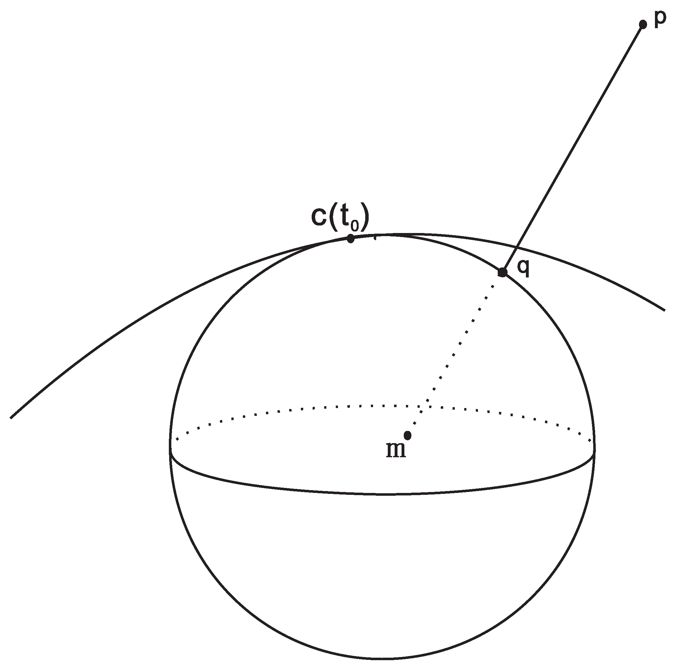
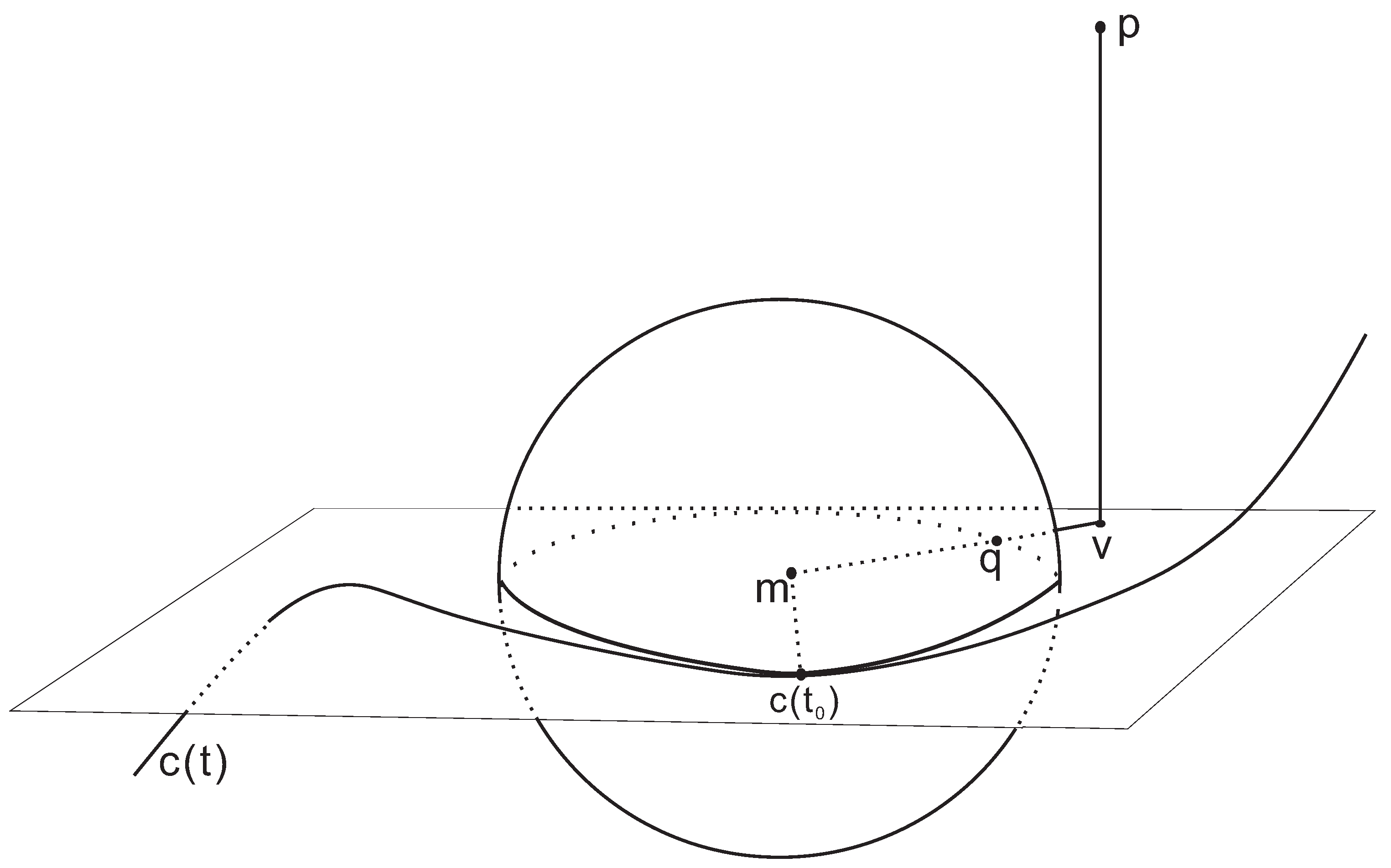
2. Orthogonal Projection onto a Spatial Parametric Curve

Assume that $c\left(t\right)$ is a $C^2$ curve in three-dimensional Euclidean space $R^3$, and p is a test point. The scalar product of vectors $x,y\in R^3$ will be denoted by $⟨x,y⟩$, and the norm of a vector x by $∥x∥$. The curve’s curvature will be denoted by the symbol k which is computed by the formula ${\displaystyle k\left(t\right)=\frac{∥c^{\prime }\left(t\right)\times c^{″}\left(t\right)∥}{{∥c^{\prime }\left(t\right)∥}^3}}$. Recall that the osculating sphere has a radius $\left|1/k\right|$ and its center is determined by Equation (10).

A first-order geometric iterative method which computes the footpoint q of the test point p is as follows: The intersection of the osculating sphere $\overline{s}$ of the curve $c\left(t\right)$ at $t=t_0$ and the line segment which connects the test point p and the center of the osculating sphere is the footpoint q. The footpoint q is expressed in terms of $c\left(t_0\right)$ and the derivative $c^{\prime }\left(t_0\right)$ (see Figure 1):

$$q=c\left(t_0\right)+\Delta t{c}^{\prime }\left(t_0\right)$$

(1)

Then,

$$\Delta t=\frac{⟨c^{\prime }\left(t_0\right),q-c\left(t_0\right)⟩}{⟨c^{\prime }\left(t_0\right),c^{\prime }\left(t_0\right)⟩}$$

(2)

Figure 1. Illustration of the first-order geometric iteration for computing the minimum distance between a point and a spatial parametric curve.

We increase $t_0$ by $\Delta t$ and repeat the above procedure until $\Delta t$ is less than a given tolerance. Thus, we can compute the projection of the test point p onto the curve in a simple way.

In order to improve the efficiency of the geometric iteration, we present a second-order iterative method to compute the minimum distance between the test point p and a spatial parametric curve $c\left(t\right)$. This geometric second-order iterative method which computes the footpoint q of the test point p is as follows: orthogonal projecting of the test point p onto an osculating plane of the spatial parametric curve $c\left(t\right)$ at $t=t_0$ yields a point v. Then, the intersection of an osculating sphere $\overline{s}$ and a line segment which connects the point v and a center of the osculating sphere $\overline{s}$ is the footpoint q. The intersection of the osculating plane of the spatial parametric curve $c\left(t\right)$ at $t=t_0$ and the osculating sphere $\overline{s}$ of the spatial parametric curve $c\left(t\right)$ at $t=t_0$ is a osculating circle $\overline{c}$ of the spatial parametric curve $c\left(t\right)$ at $t=t_0$. We assume that, for the moment, the osculating circle $\overline{c}$ is parameterized such that it has the same Taylor polynomial as the curve $c\left(t\right)$. Similar to the first-order geometric iterative method, we get (see Figure 2):

$$q=\overline{c}(t_0+\Delta t)=c\left(t_0\right)+\Delta t{c}^{\prime }\left(t_0\right)$$

(3)

Then

$$\Delta t=\frac{⟨c^{\prime }\left(t_0\right),q-c\left(t_0\right)⟩}{⟨c^{\prime }\left(t_0\right),c^{\prime }\left(t_0\right)⟩}$$

(4)

Figure 2. Illustration of the second-order geometric iteration for computing the minimum distance between a point and a spatial parametric curve.

We increase $t_0$ by $\Delta t$ and repeat the above procedure until $\Delta t$ is less than a given tolerance. This equation now can be used to compute the parameter increment $\Delta t$. Iteration yields a second-order algorithm for computing the footpoint q which is determined by the given parameter value. This algorithm also fits to solve the inversion problem, e.g., computing the parameter value t for a point which is known to lie on the curve.

Remark 1. 

During the process of calculating the footpoint q, since the footpoint q only depends on the projection point v, which is the projection of the test point p onto the osculating plane, while the osculating plane is given by the osculating sphere $\overline{s}$ of the spatial parametric curve $c\left(t\right)$ at $t=t_0$. In addition, it is not necessary to compute the osculating circle $\overline{c}$ which is the intersection of the osculating plane and the osculating sphere $\overline{s}$ of the spatial parametric curve $c\left(t\right)$ at $t=t_0$. Hence, our proposed method improves the efficiency and stability for computing q.

Remark 2. 

If the denominator of the iterative Equation (4) becomes 0, i.e., $c^{\prime }\left(t_0\right)=0$ for some non-negative integer, first, we compute the distance between the test point p and the point $c\left(t_0\right)$ of the spatial parametric curve $c\left(t\right)$, namely, $d_1=∥p-c\left(t_0\right)∥$. At the same time, we employ the parameter perturbation method, and the parameter $t_0$ is incremented by a small positive constant ε, i.e., $t_0=t_0+\epsilon$, so the iteration can continue. In the process of the iteration, if the derivative of the spatial parametric curve $c\left(t\right)$ at $t=t_0$ is zero, we adopt the same processing method. Finally, $d=min\{d_1,d_2,d_3,\dots \}$ is the minimum distance between the test point p and the spatial parametric curve $c\left(t\right)$.

Remark 3. 

If the curvature k of the spatial parametric curve $c\left(t\right)$ at $t=t_0$ becomes 0, i.e., for some non-negative integer, the processing method of this special case is similar to the method in Remark 1.

Remark 4. 

The iterative method in the iterative Equation (4) is an orthogonal projection method which projects a test point onto a spatial parametric curve $c\left(t\right)$. For the multiple orthogonal points situation, we use the method in the reference [14] to calculate all the orthogonal projection points, and then calculate all the distances between the test point p and all the orthogonal projection points. In the end, the minimum distance is the minimum one of all the distances between the test point p and all the orthogonal projection points.

3. Convergence Analysis

In this section, we consider the convergence analysis of the iterative technique given in Equation (4). Namely, we consider the problem of projecting a point onto a spatial parameter curve.

In order to prove that the method defined by Equation (4) is quadratically convergent, we firstly derive the expression of the foot point q. We assume that the parameter α is the corresponding parameter which we get from the orthogonal projection of a test point p onto a parameter curve $c\left(t\right)$. According to the calculation of the minimum distance between a point and a spatial parameter curve, we can get the following relationship

$$⟨p-h,\mathbf{n}⟩=0$$

(5)

where $h=(f_1\left(\alpha \right),f_2\left(\alpha \right),f_3\left(\alpha \right))$ and the tangent vector. $\mathbf{n}=(f_1^{\prime }\left(\alpha \right),f_2^{\prime }\left(\alpha \right),f_3^{\prime }\left(\alpha \right))$ Therefore, the Equation (5) can be rewritten as

$$⟨p-c\left(\alpha \right),\mathbf{n}⟩=0$$

(6)

The unit normal vector, the curvature and the radius of the osculating sphere of the curve $c\left(t\right)$ can be represented respectively by the following formulas,

$$\beta \left(t\right)=\gamma \left(t\right)\times \Omega \left(t\right)=\frac{∥c^{\prime }\left(t\right)∥}{∥c^{\prime }\left(t\right)\times c^{″}\left(t\right)∥}{c}^{″}\left(t\right)-\frac{⟨c^{\prime }\left(t\right),c^{″}\left(t\right)⟩}{∥c^{\prime }\left(t\right)∥·∥c^{\prime }\left(t\right)\times c^{″}\left(t\right)∥}{c}^{\prime }\left(t\right)$$

(7)

$$k\left(t\right)=\frac{∥c^{\prime }\left(t\right)\times c^{″}\left(t\right)∥}{{∥c^{\prime }\left(t\right)∥}^3}=\frac{B\left(t\right)}{A{\left(t\right)}^3}$$

(8)

$$R\left(t\right)=\left|\frac{1}{k\left(t\right)}\right|=\left|\frac{A{\left(t\right)}^3}{B\left(t\right)}\right|$$

(9)

where ${\displaystyle \gamma \left(t\right)=\frac{c^{\prime }\left(t\right)\times c^{″}\left(t\right)}{∥c^{\prime }\left(t\right)\times c^{″}\left(t\right)∥}}$, ${\displaystyle \Omega \left(t\right)=\frac{c^{\prime }\left(t\right)}{∥c^{\prime }\left(t\right)∥}}$, $A\left(t\right)=∥c^{\prime }\left(t\right)∥$ $B\left(t\right)=∥c^{\prime }\left(t\right)\times c^{″}\left(t\right)∥$.

In this paper, we prove the case in which ${\displaystyle R\left(t\right)=\left|\frac{1}{k\left(t\right)}\right|=\frac{1}{k\left(t\right)}}$. In addition, the proof method is also valid for the case ${\displaystyle R\left(t\right)=\left|\frac{1}{k\left(t\right)}\right|=\frac{-1}{k\left(t\right)}}$ only with an opposite sign. The center of the osculating sphere of the spatial parametric curve $c\left(t\right)$ is defined by

$$\mathrm{m}\left(t\right)=c\left(t\right)+\beta \left(t\right)/k\left(t\right)$$

(10)

Now substituting Equations (7) and (8) into Equation (10), we obtain

$$\begin{array}{cc}\hfill \mathrm{m}\left(t\right)=& c\left(t\right)+\frac{A^3\left(t\right)}{B\left(t\right)}[\frac{A\left(t\right)}{B\left(t\right)}{c}^{″}\left(t\right)-\frac{⟨c^{\prime }\left(t\right),c^{″}\left(t\right)⟩}{A\left(t\right)B\left(t\right)}{c}^{\prime }\left(t\right)]\hfill \\ \hfill =& c\left(t\right)+\frac{A{\left(t\right)}^2}{B{\left(t\right)}^2}[c^{″}\left(t\right)-A\left(t\right)⟨c^{\prime }\left(t\right),c^{″}\left(t\right)⟩c^{\prime }\left(t\right)]\hfill \end{array}$$

(11)

The equation of the osculating plane of the spatial parametric curve $c\left(t\right)$ can be expressed as following

$$⟨x-c\left(t\right),\gamma \left(t\right)⟩=0$$

(12)

where $x=(x,y,z)$. Assume that the orthogonal projection of the test point p onto the osculating plane of the spatial parametric curve $c\left(t\right)$ yields a point v. Thus, the equation of line segment $\overrightarrow{p\mathrm{v}}$ is the following

$$x=p+\frac{\gamma \left(t\right)}{∥\gamma \left(t\right)∥}w$$

(13)

where w is the parameter. Substituting Equation (13) into (12), we can obtain the parameter w as the following,

$$⟨p-c\left(t\right),\gamma \left(t\right)⟩+w∥\gamma \left(t\right)∥=0$$

hence,

$$w=\frac{⟨\gamma \left(t\right),c\left(t\right)-p⟩}{∥\gamma \left(t\right)∥}$$

(14)

Substituting Equation (14) into Equation (13), we can get the coordinate value of the projection point v as the following

$$\mathrm{v}=p+\frac{\gamma \left(t\right)}{∥\gamma \left(t\right)∥}w$$

(15)

where parameter w is the same as that of Equation (14). The corresponding parametric equation of the line segment that connects the projecting point v and the center $\mathrm{m}\left(t\right)$ of the osculating sphere can be expressed as

$$x=\mathrm{v}+\left(\mathrm{m}\right(t)-\mathrm{v})u\left(t\right)$$

(16)

where $u\left(t\right)$ is a parameter for the line segment between the center m of the osculating sphere and the projection point v. We know that the equation of the osculating sphere is

$$∥x-\mathrm{m}∥=R$$

(17)

Because the footpoint q is the intersection of the line segment Equation (16) and the osculating sphere Equation (17), we get

$$∥\mathrm{v}+\left(\mathrm{m}\right(t)-\mathrm{v})u\left(t\right)-\mathrm{m}\left(t\right)∥=R\left(t\right)$$

(18)

i.e., $\left|1-u\left(t\right)\right|∥\mathrm{m}\left(t\right)-\mathrm{v}∥=R\left(t\right)$.

There, we have

$$u\left(t\right)=1\pm \frac{R\left(t\right)}{∥\mathrm{m}\left(t\right)-\mathrm{v}∥}$$

(19)

Because the footpoint q is located between the center $\mathrm{m}\left(t\right)$ of the osculating sphere and the projecting point v, so the parameter $u\left(t\right)$ should be

$$u\left(t\right)=1-\frac{R\left(t\right)}{∥\mathrm{m}\left(t\right)-\mathrm{v}∥}$$

(20)

Substituting Equation (20) into Equation (18), we get the footpoint coordinate

$$q\left(t\right)=\mathrm{v}+\left(\mathrm{m}\right(t)-\mathrm{v})u\left(t\right)$$

(21)

Secondly, we present the proof of the theorem, our proof method used in the following is distinguished from that literature [23]. We use the method of the numerical analysis similar to those in the literature [24,25,26,27,28].

Theorem 1 

Let $q\left(t\right)-c\left(t\right)$ be a three-dimensional real parametric curve function, assume that $q\left(t\right)-c\left(t\right)$ has first, second derivatives in an interval I. If $q\left(t\right)-c\left(t\right)$ has a simple root $\alpha \in I$, and $t_n$ is close to α, then the iterative method Equation (4) is quadratically convergent.

Proof. 

Let $e_n=t_n-\alpha$, and let α be a simple root of $q\left(t\right)-c\left(t\right)=0$, i.e., $q\left(\alpha \right)-c\left(\alpha \right)=0,q^{\prime }\left(\alpha \right)-c^{\prime }\left(\alpha \right)\ne 0.$ For $c\left(t\right)$, using the Taylor’s expansion around α, we get

$$c\left(t_n\right)={\mathrm{B}}_0+{\mathrm{B}}_1{e}_n+{\mathrm{B}}_2{e}_n^2+o\left(e_n^3\right)$$

(22)

$$c^{\prime }\left(t_n\right)={\mathrm{B}}_1+2{\mathrm{B}}_2{e}_n+o\left(e_n^2\right)$$

(23)

$$c^{″}\left(t_n\right)=2{\mathrm{B}}_2+o\left(e_n\right)$$

(24)

where ${\mathrm{B}}_i=(1/i!)c^{\left(i\right)}\left(\alpha \right),i=0,1,2,\dots$. ☐

For convenience, we employ the symbolic computation of the Maple 18 package to compute the Taylor’s expansion as follows. Combining the derivation Equation (7)–(21) with the condition of orthogonal projection Equation (6), as well as Equation (22)–(24), and after simplifying, we get a formula of the parameter increment $\Delta t$,

$$\Delta t=-e_n+\frac{⟨{\mathrm{B}}_1,{\mathrm{B}}_2⟩(⟨{\mathrm{B}}_1,{\mathrm{B}}_1⟩+4⟨{\mathrm{B}}_2,p⟩-4⟨{\mathrm{B}}_0,{\mathrm{B}}_2⟩)}{⟨{\mathrm{B}}_1,{\mathrm{B}}_1⟩(⟨{\mathrm{B}}_1,{\mathrm{B}}_1⟩-2⟨{\mathrm{B}}_2,p⟩+2⟨{\mathrm{B}}_0,{\mathrm{B}}_2⟩)}{e}_n^2+o\left(e_n^3\right)$$

(25)

since

$$\Delta t=e_{n+1}-e_n.$$

(26)

Substituting Equation (26) into Equation (25), we can get the following error equation

$$e_{n+1}=\frac{⟨{\mathrm{B}}_1,{\mathrm{B}}_2⟩(⟨{\mathrm{B}}_1,{\mathrm{B}}_1⟩+4⟨{\mathrm{B}}_2,p⟩-4⟨{\mathrm{B}}_0,{\mathrm{B}}_2⟩)}{⟨{\mathrm{B}}_1,{\mathrm{B}}_1⟩(⟨{\mathrm{B}}_1,{\mathrm{B}}_1⟩-2⟨{\mathrm{B}}_2,p⟩+2⟨{\mathrm{B}}_0,{\mathrm{B}}_2⟩)}{e}_n^2+o\left(e_n^3\right)$$

(27)

This means that the method defined by Equation (4) is quadratically convergent.

In the following, we prove that Equation (4) is globally convergent.

Theorem 2 

For the test point p, if there only exists one orthogonal projection point, then the Equation (4) is globally convergent.

Proof. 

This proof is analogous to the proof in the literature [29,30]. If we start from an initial point on the left-hand side of α, then the footpoint q must be located on the right-hand side of the initial point, so $\Delta t$ is a positive real number. By Equation (4), we define the following iterative sequence:

$$t_n=t_{n-1}+\Delta t_{n-1}$$

(28)

where

$$\Delta t_{n-1}=\frac{⟨c^{\prime }\left(t_{n-1}\right),q-c\left(t_{n-1}\right)⟩}{⟨c^{\prime }\left(t_{n-1}\right),c^{\prime }\left(t_{n-1}\right)⟩}$$

For $t_n<\alpha$, the sequence $\left\{t_n\right\}$ is strictly monotonic increasing. If $t_n>\alpha$, and then, by at most three iterations, the sequence $\left\{t_n\right\}$ converges to α. We should note that this iterative sequence $\left\{t_n\right\}$ is similar to an attenuated pendulum. Moreover, if the initial point is to the right-hand side of the root α, the convergence works in a similar way.

On the other hand, the footpoint q is jointly determined by the center of the osculating sphere and the orthogonal projection point v. Furthermore, the footpoint q is always associated with the test point p, but it is not restricted by the initial iteration point. Therefore, Equation (4) is globally convergent. ☐

Remark 5. 

The global convergence of the method in the iterative Equation (4) only requires that $c\left(t\right)$ is $C^2$, however, the global convergence of the method in the literature [26,27,28] must satisfy some stronger sufficient conditions.

4. Numerical Examples

This section shows the numerical evidence comparing the behavior of the Newton’s iterative algorithm and our second-order geometric algorithm discussed above.

Example 1. 

We consider the curve $c\left(t\right)=(t,t^2,sin\left(t\right))$. Table 1 shows the results of Newton’s iteration and geometric iteration. The experimental data shows our second-order algorithm has good convergence and robustness, but the convergence rate of Newton’s method is sometimes slower.

Table 1. Stepsizes Δt₁, Δt₂ in Example 1 for the Newton’s method and our second-order algorithm.

p = (1, 1, 1), t0 = 1.5
Step	1	2	3	4	5	6	7
Δt1	−3.4e−1	−1.2e−1	−1.7e−2	−2.9e−4	−8.3e−8	−6.7e−15	0
Δt2	−4.2e−1	−6.3e−2	−1.3e−3	−5.0e−7	−7.8e−14	7.3e−18	0
p = (1, 1, 1), t0 = −0.85
Step	1	2	3	4	5	6	7
Δt1	1.03	6.3	−2.1	−1.43	−9.1e-1	−5.6e−1	−3.1e−1
Step	8	9	10	11	12
Δt1	−1.1e−2	−1.3e−4	−1.6e−8	−2.2e−16	0
Step	1	2	3	4	5	6	7
Δt2	1.2	6.5e−1	1.2e−2	−4.1e−5	−5.2e−10	7.4e−18	0

Table 1. Stepsizes Δt₁, Δt₂ in Example 1 for the Newton’s method and our second-order algorithm.

p = (1, 1, 1), t0 = 1.5
Step	1	2	3	4	5	6	7
Δt1	−3.4e−1	−1.2e−1	−1.7e−2	−2.9e−4	−8.3e−8	−6.7e−15	0
Δt2	−4.2e−1	−6.3e−2	−1.3e−3	−5.0e−7	−7.8e−14	7.3e−18	0
p = (1, 1, 1), t0 = −0.85
Step	1	2	3	4	5	6	7
Δt1	1.03	6.3	−2.1	−1.43	−9.1e-1	−5.6e−1	−3.1e−1
Step	8	9	10	11	12
Δt1	−1.1e−2	−1.3e−4	−1.6e−8	−2.2e−16	0
Step	1	2	3	4	5	6	7
Δt2	1.2	6.5e−1	1.2e−2	−4.1e−5	−5.2e−10	7.4e−18	0

Example 2. 

We consider the curve $c\left(t\right)=(t,sin(t),0)$. Table 2 shows the results of Newton’s iteration and geometric iteration. The experimental data shows that our second-order algorithm has good convergence and robustness, the convergence of Newton’s method is sensitive to the choice of initial values and unstable compared with our Euqation (4). Note that NC in Table 2 means the Newton’s second-order iterative method does not converge to the root.

Table 2. Stepsizes Δt₁, Δt₂ in Example 2 for the Newton’s method and our second-order algorithm.

p = (2, 2, 0), t0 = −0.32
Step	1	2	3	4	5	6
Δt1	NC	NC	NC	NC	NC	NC
Δt2	1.82	2.8e−1	2.1e−3	8.3e−7	1.4e−13	0
p = (2, 2, 0), t0 = 4.2
Step	1	2	3	4	5	6	7
Δt1	NC	NC	NC	NC	NC	NC	NC
Δt2	−7.2e−1	−1.65	−4.1e−2	3.5e−4	2.5e−8	2.2e−16	0

Table 2. Stepsizes Δt₁, Δt₂ in Example 2 for the Newton’s method and our second-order algorithm.

p = (2, 2, 0), t0 = −0.32
Step	1	2	3	4	5	6
Δt1	NC	NC	NC	NC	NC	NC
Δt2	1.82	2.8e−1	2.1e−3	8.3e−7	1.4e−13	0
p = (2, 2, 0), t0 = 4.2
Step	1	2	3	4	5	6	7
Δt1	NC	NC	NC	NC	NC	NC	NC
Δt2	−7.2e−1	−1.65	−4.1e−2	3.5e−4	2.5e−8	2.2e−16	0

5. Conclusions

This paper investigates the problem related to a point projection onto spatial parametric curves by using curvature information. This method is globally second-order convergence. Experimental results show that the algorithm under consideration is robust and efficient. An area for future research is to develop a more efficient algorithm with higher-order convergence for computing the minimum distance between a point and a spatial parametric curve.

References

- Ma, Y.L.; Hewitt, W.T. Point inversion and projection for NURBS curve and surface: Control polygon approach. Comput. Aided Geometric Des. 2003, 20, 79–99. [Google Scholar] [CrossRef]
- Yang, H.P.; Wang, W.P.; Sun, J.G. Control point adjustment for B-spline curve approximation. Comput. Aided Design 2004, 36, 639–652. [Google Scholar] [CrossRef]
- Johnson, D.E.; Cohen, E. A Framework for efficient minimum distance computations. In Proceedings of IEEE Intemational Conference on Robotics & Automation, Leuven, Belgium, 16–20 May 1998.
- Piegl, L.; Tiller, W. Parametrization for surface fitting in reverse engineering. Comput. Aided Des. 2001, 33, 593–603. [Google Scholar] [CrossRef]
- Pegna, J.; Wolter, F.E. Surface curve design by orthogonal projection of space curves onto free-form surfaces. J. Mech. Design ASME Trans. 1996, 118, 45–52. [Google Scholar] [CrossRef]
- Besl, P.J.; McKay, N.D. A method for registration of 3-D shapes. IEEE Trans. Pattern Anal. Mach. Intell. 1992, 14, 239–256. [Google Scholar] [CrossRef]
- Mortenson, M.E. Geometric Modeling; Wiley: New York, NY, USA, 1985. [Google Scholar]
- Zhou, J.M.; Sherbrooke, E.C.; Patrikalakis, N. Computation of stationary points of distance functions. Engin. Comput. 1993, 9, 231–246. [Google Scholar] [CrossRef]
- Johnson, D.E.; Cohen, E. Distance extrema for spline models using tangent cones. In Proceedings of the 2005 Conference on Graphics Interface, Victoria, BC, Canada, 9–11 May 2005.
- Hartmann, E. On the curvature of curves and surfaces defined by normalforms. Comput. Aided Geometric Des. 1999, 16, 355–376. [Google Scholar] [CrossRef]
- Limaien, A.; Trochu, F. Geometric algorithms for the intersection of curves and surfaces. Comput. Gr. 1995, 19, 391–403. [Google Scholar]
- Polak, E.; Royset, J.O. Algorithms with adaptive smoothing for finite minimax problems. J. Optim. Theory Appl. 2003, 119, 459–284. [Google Scholar] [CrossRef]
- Press, W.H.; Teukolsky, S.A.; Vetterling, W.T.; Flannery, B.P. Numerical Recipes in C: The Art of Scientific Computing; Cambridge University Press: NewYork, NY, USA, 1992. [Google Scholar]
- Elber, G.; Kim, M.S. Geometric Constraint solver using multivariate rational spline functions. In Proceedings of the Sixth ACM Symposiumon Solidmodeling and Applications, New York, NY, USA, 1 May 2001; pp. 1–10.
- Patrikalakis, N.; Maekawa, T. Shape Interrogation for Computer Aided Design and Manufacturing; Springer: Berlin, Germany, 2001. [Google Scholar]
- Chen, X.D.; Zhou, Y.; Shu, Z.Y.; Su, H.; Paul, J.C. Improved Algebraic Algorithmon Point Projection for Bézier Curves; The University of Iowa: Des Moines, IA, USA, 2007. [Google Scholar]
- Selimovic, I. Improved algorithms for the projection of points on NURBS curves and surfaces. Comput. Aided Geometric Des. 2006, 23, 439–445. [Google Scholar] [CrossRef]
- Boehm, W. Inserting new knots into B-spline curves. Comput. Aided Des. 1980, 12, 199–201. [Google Scholar] [CrossRef]
- Cohen, E.; Lyche, T.; Riesebfeld, R. Discrete B-splines and subdivision techniques in computer-aided geometric design and computer graphics. Comput. Gr. Image Process. 1980, 14, 87–111. [Google Scholar] [CrossRef]
- Piegl, L.; Tiller, W. The NURBS Book; Springer: New York, NY, USA, 1995. [Google Scholar]
- Chen, X.D.; Yong, J.H.; Wang, G.Z.; Paul, J.C.; Xu, G. Computing the minimum distance between a point and a NURBS curve. Comput. Aided Des. 2008, 40, 1051–1054. [Google Scholar] [CrossRef]
- Hu, S.M.; Wallner, J. A second-order algorithm for orthogonal projection onto curves and surfaces. Comput. Aided Geometric Des. 2005, 22, 251–260. [Google Scholar] [CrossRef]
- Schulz, C. Bézier clipping is quadratically convergent. Comput. Aided Geometric Des. 2009, 26, 61–74. [Google Scholar] [CrossRef]
- Li, X.W.; Mu, C.L.; Ma, J.W.; Wang, C. Sixteenth-order method for nonlinear equations. Appl. Math. Comput. 2010, 215, 3754–3758. [Google Scholar] [CrossRef]
- Liang, J.; Li, X.W.; Wu, Z.W.; Zhang, M.S.; Wang, L.; Pan, F. Fifth-order iterative method for solving multiple roots of the highest multiplicity of nonlinear equation. Algorithms 2015, 8, 656–668. [Google Scholar] [CrossRef]
- Cordero, A.; Hueso, J. L.; Martínez, E.; Torregrosa, J. R. A modified Newton-Jarratt’s composition. Numer. Algor. 2010, 55, 87–99. [Google Scholar] [CrossRef]
- Grau-Sanchez, M.; Noguera, M.; Amat, S. On the approximation of derivatives using divided difference operators preserving the local convergence order of iterative methods. J. Comput. Appl. Math. 2013, 237, 363–372. [Google Scholar] [CrossRef]
- Ostrowski, A.M. Solutions of Equations and Systems of Equations; Academic Press: New York, NY, USA, 1966. [Google Scholar]
- Melmant, A. Geometry and Convergence of Euler’s and Halley’s Methods. SIAM Rev. 1997, 39, 728–735. [Google Scholar] [CrossRef]
- Traub, J.F. A Class of Globally Convergent Iteration Functions for the Solution of Polynomial Equations. Math. Comput. 1966, 20, 113–138. [Google Scholar] [CrossRef]
© 2016 by the authors; licensee MDPI, Basel, Switzerland. This article is an open access article distributed under the terms and conditions of the Creative Commons by Attribution (CC-BY) license (http://creativecommons.org/licenses/by/4.0/).