Quantitative Trait Loci Mapping Problem: An Extinction-Based Multi-Objective Evolutionary Algorithm Approach

Abstract

The Quantitative Trait Loci (QTL) mapping problem aims to identify regions in the genome that are linked to phenotypic features of the developed organism that vary in degree. It is a principle step in determining targets for further genetic analysis and is key in decoding the role of specific genes that control quantitative traits within species. Applications include identifying genetic causes of disease, optimization of cross-breeding for desired traits and understanding trait diversity in populations. In this paper a new multi-objective evolutionary algorithm (MOEA) method is introduced and is shown to increase the accuracy of QTL mapping identification for both independent and epistatic loci interactions. The MOEA method optimizes over the space of possible partial least squares (PLS) regression QTL models and considers the conflicting objectives of model simplicity versus model accuracy. By optimizing for minimal model complexity, MOEA has the advantage of solving the over-fitting problem of conventional PLS models. The effectiveness of the method is confirmed by comparing the new method with Bayesian Interval Mapping approaches over a series of test cases where the optimal solutions are known. This approach can be applied to many problems that arise in analysis of genomic data sets where the number of features far exceeds the number of observations and where features can be highly correlated.

1. Introduction

Advances in biological technology are generating an exponential growth in the amount of genomic data available for analysis. Processing this data requires pattern classification and feature selection methods that can identify those features that are significant, in addition to eliminating redundant and irrelevant features. Effective methods are especially needed that function over very large data sets with thousands of features, such as genome databases of living organisms. An important genome data analysis task is to identify subsets of genes that affect a specific phenotypic characteristic, such as infectious and inflammatory diseases [1], economically important traits in agricultural products [2], or in cancer prognosis [3]. Phenotypic characteristics can be binary, such as whether or not an individual has a particular disease, or quantitative and continuous, such as the weight of a species [4] or the number of bristles on Drosophila melanogaster [5].

Quantitative traits in organisms are formed during development by the interaction of many genes located throughout the genome and distributed over multiple chromosomes. Experiential techniques that study quantitative traits determine the location of each relevant genes, termed loci, rather than the genes directly. So the problem of identifying the set of genes (polygenes) that affect the variation of a quantitative trait is defined in terms of the loci of those genes, and referred to as Quantitative Trait Loci (QTL) problem [4]. Knowing the locations and effects of QTLs enables scientists to understand the biochemical basis of traits and how these traits may have evolved through the time. There is great economic value in solving the QTL problem for specific traits of commercial organisms since these traits may then be manipulated to improve yield.

Mendel in 1866 [6] was the first to introduce the quantitative trait loci concept. He suggested that the color of flowers can be influenced by several genetic factors. Some years later, in 1923, Sax [7] studied the relation of seed weight and seed coat color in beans demonstrating that multiple genes control these bean phenotypes.

The use of genetic markers was introduced by Thoday in 1961 [8] as a means to map different groups of genes that together control a quantitative trait. Biochemical markers characterize and identify QTLs responsible for variation in quantitative traits by identifying similarities and differences over samples of DNA and their corresponding phenotypes. Techniques that utilized dominant markers have the advantage over co-dominant methods since they allow for the analysis of many loci per experiment. An earlier method, Random Amplification of Polymorphic DNA (RAPD) was slow and cumbersome since it requires a large amount of sample DNA along with steps to produce the gene loci present. New techniques such as amplified fragment length polymorphism or AFLP utilize high-throughput sequencing to speedup the process. Many authors have applied these techniques in their research to study economically significant organisms like: maize (see [9,10,11]), tomatoes (see [12,13]), and rice (see [14]).

2. QTL Mapping Problem Description

Let P be a population of size n individuals that exhibit a quantitative trait. For individual i, the magnitude of the trait (measured value of the trait) is defined as $t_i$. There exist a set of k genetic markers implemented with molecular tags, that denote the presence of locus on the chromosomes of specific alleles in the individuals. An experiment yields a vector $M_i$ of genetic markers present in individual i and the magnitude of the individual’s trait $t_i$. For each specific experiment $M_{i,j}$ denotes the value of marker $j,1\le j\le k$ in individual i.

The model sought by geneticists is to identify the loci of DNA that control the quantitative trait, the contribution of each locus to the magnitude of the trait, and the interaction among the loci. As an example, a phenotype may be shaped by many independent loci distributed over multiple chromosomes, or by a few loci within a single chromosome. There may be little or no interaction among the genes at those loci so that their effect on the trait can be treated as independent and additive; or interaction may be epistatic where multiple genes interact to control the trait. The complexity of the QTL mapping problem depends whether the genes are treated as independent or epistatic. First consider the case when genes are independent, then the model can be represented as a weighted sum and determined by partial least squares (PLS) linear regression [15]:

$${\widehat{t}}_i={\beta }_0+\sum _{j=1}^k{\beta }_j{M}_{i,j}$$

(1)

where ${\widehat{t}}_i$ is the predicted value of the trait, ${\beta }_0$ is the error term (bias) and the ${\beta }_j$ values are the weights or regression coefficients of the model over all individual genes. The loci present in individual i, $M_{i,j}$ determine which weights contribute to the magnitude of the trait. The PLS method determines the model parameters ${\beta }_j$ by minimizing the squared error ${(t_i-{\widehat{t}}_i)}^2$ over the population of n individuals. To extend the method to epistatic interactions we consider all pairwise markers in addition to individual markers:

$${\widehat{t}}_i={\beta }_0+\sum _{j=1}^k{\beta }_j{M}_{i,j}+\sum _{u=1}^k\sum _{v=u+1}^k{\beta }_{u,v}{M}_{i,u}{M}_{i,v}$$

(2)

In this model, there are a total of $(k^2+k)/2$ regression coefficients, a number that will most likely exceed the number of samples n. The β values for additive or epistatic interactions may be positive, signalling synergistic influence or negative signalling antagonistic influence.

2.1. Statistical PLS Methods

Like every linear statistical method, PLS has some advantages and disadvantages; its main advantage is that it can be accurate when the sample size n and number of predictor variables is small, and there are few irrelevant markers. Another reason that makes PLS regression a good option for small QTL mapping problems is its robustness against environmental variation in the data and missing data; also it can handle multi-collinearity among the genes [16].

However, this regression method is unsuitable for larger problems when the number of predictor variables grows, particularly in the epistatic model, where the number grows with the square of the number of markers. The problems are two fold: first the solution will over-fit the data due to the excess of parameters and secondly, the method becomes unable to accurately discriminate those genes that control the trait from irrelevant genes. While hybrid methods have been introduced to ameliorate these problems [17,18,19], the application of the PLS method in QTL mapping is limited [20]. This paper presents a new hybrid method that overcomes both these limitations of PLS while retaining the advantages. The method finds accurate and compact QTL epistatic PLS models with large k and n.

2.2. Genetic Algorithms QTL Solution Methods

Genetic Algorithms (GAs) are a subset of evolutionary algorithms that have been proved effective in solving QTL mapping problem. Carlborg et al. [21] proposed a GA-based approach for searching the QTL space and demonstrated that for smaller problem sizes their method’s accuracy was comparable to an exhaustive search for locating QTL. Zhang and Horvath [22] suggested a hybrid genetic algorithm to optimize a fitness function relating genetic markers to quantitative traits in F2 mice. Lee et al. [23] used GA for haplotype reconstruction in locating QTL where they demonstrated an improvement in efficiency and reliability compared to SimWalk 2 [24].

3. Solving QTL by Multi-Criteria Optimization

Rather than produce a model that attempts to identify $(k^2+k)/2$ model parameters, most of which will be close to zero, the new method introduced here identifies a subset of those parameters that best explain the data and are biologically relevant. An evolutionary algorithm is applied to search the powerset of model parameters maximizing the R squared measure (defined below) as a goodness of fit. To provide a search bias for parsimony, an additional fitness criteria is introduced so that the number of model parameters is minimized. The multi-objective search method applies two objectives: minimize the complexity (model parameters) and maximize the quality of fit to the data ($R^2$).

3.1. QTL Solution Representation

A model solution is a subset of single loci and pairs of epigenetic loci along with their corresponding PLS weight parameters. The set of single loci solution for additive influence is represented as a set of model parameters $B_a\in \mathcal{P}\left(B^1\right)$, where $B^1=\{{\beta }_j:1\le j\le k\}$. The set of epistatic solution loci is $B_e\in \mathcal{P}\left(B^2\right)$, where $B^2=\{{\beta }_{u,v}:1\le u\le k,u<v<k\}$. The overall solution is the union of these two sets $B_s=B_a\cup B_e$. Given that $B_{\diamond }\in \mathcal{P}\left(B^1\right)$ then for additive genes $B_a$ is defined:

$$B_a=\underset{B_{\diamond }}{argmax}\left\{\sum _{i=1}^n{\left(t_i-{\beta }_0-\sum _{{\beta }_j\in B_{\diamond }}{\beta }_j{M}_{i,j}\right)}^2\right\}$$

(3)

such that the maximization criteria is defined as:

$$R^2=1-\frac{{\sum }_{i=1}^n{\left(t_i-{\beta }_0-{\sum }_{{\beta }_j\in B_a}{\beta }_j{M}_{i,j}\right)}^2}{{\sum }_{i=1}^n{\left(t_i-\overline{t}\right)}^2}$$

(4)

where $\overline{t}=\frac{1}{n}{\sum }_{i=1}^n{t}_i$, the mean trait outcome and ${\sum }_{i=1}^n{\left(t_i-\overline{t}\right)}^2$ is the total outcome variation. $R^2$ lies between 0 and 1, when $R^2=1$ the model is perfectly fitted.

Given that $B_{*}\in \mathcal{P}\left(B^2\right)$, then when we include epistatic genes, the overall solution $B_s$ is defined:

$$B_s=\underset{B_{\diamond },B_{*}}{argmax}\left\{\sum _{i=1}^n{\left(t_i-{\beta }_0-\sum _{{\beta }_j\in B_{\diamond }}{\beta }_j{M}_{i,j}-\sum _{{\beta }_{u,v}\in B_{*}}{\beta }_{u,v}{M}_{i,u}{M}_{i,v}\right)}^2\right\}$$

(5)

such that the maximization criteria is:

$$R^2=1-\frac{{\sum }_{i=1}^n{\left(t_i-{\beta }_0-{\sum }_{{\beta }_j\in B_{\diamond }}{\beta }_j{M}_{i,j}-{\sum }_{{\beta }_{u,v}\in B_{*}}{\beta }_{u,v}{M}_{i,u}{M}_{i,v}\right)}^2}{{\sum }_{i=1}^n{\left(t_i-\overline{t}\right)}^2}$$

(6)

The genetic algorithm described below searches the space of $\mathcal{P}\left(B^1\right)\cup \mathcal{P}\left(B^2\right)$, which contains $O\left(2^{k^2}\right)$ possible solutions when considering epistatic solutions, or $O\left(2^k\right)$ when only additive solutions are considered. The aim is to identify a solution that maximizes $R^2$ in Equation (6) and minimizes the complexity of the solution $|B_s|$. These two optimization criteria are in conflict because the more parameters employed in the model, the better the fit to the data. However, too many parameters result in fitting the inevitable environmental variation that exists in the data and produces biologically meaningless results. It is this problem of over fitting and parameter selection that the work here is designed to solve. There follows a review of multi-objective optimization approaches and the specific genetic algorithm applied to solve the QTL problem.

3.2. Multi-objective Optimization Methods

Due to the ability of Evolutionary Algorithms (EAs) to explore massive search spaces and to identify near-global optima in reasonable time, these algorithms have been employed widely. However, EAs can lead to unwanted solution complexity when used for fitting models, and in this case additional techniques must be employed to manage the tradeoff between the accuracy and the parsimony of a solution model. The Multi-Objective Genetic Algorithms (MOGAs), proposed by Fonseca and Fleming [25], is especially appropriate to solve this problem. Here, accuracy and parsimony are treated as conflicting optimization criteria and multiple model solutions are found, each on a different point of the tradeoff. The MOGAs apply the concept of dominated solutions to seek a population of near-Pareto optimal solutions that lie along the Pareto optimal frontier. The definition of the dominated solution described in [25] is as follows:

For two solutions S1 and S2, a solution S2 is said dominated by the other solution S1 (i.e., S1 is a non-dominated solution), if the below conditions are satisfied:

• The solution S1 is no worse than S2 in all objectives.
• The solution S1 is strictly better than S2 in at least one objective.

3.3. Extinction-Based Evolutionary Algorithm

This work employs a specialization of evolutionary algorithms that is specifically designed to maintain a high genetic diversity within the solution population to avoid premature convergence to suboptimal local maxima [26]. Premature convergence due to loss of diversity is avoided by employing extinction, where much of the population is periodically eliminated and replaced with new solutions [27,28,29]. While all EAs are inspired by living evolution processes, extinction methods take the analogy one step further by incorporating extinction events that are known to have occurred on Earth, such as the end of Permian era where 96% of all marine animals went extinct [30]. This event resulted in an explosive increase in the diversity of life. Extinction Evolutionary Algorithm (EEA) method, proposed by Greenwood et al. [27], uses the following scheme: In each generation, a stress factor $\eta \left(t\right)$ is generated according to $\eta \left(t\right)\sim U\left(0,0.96\right)$. Based on the following formula (assuming a minimization problem) the algorithm scales the fitness of each individual $I_i$ to the interval [α; 1] :

$$Fi{t}^{\prime }\left(i\right)=\alpha +\left(1-\alpha \right)·\frac{Fit\left(I_i\right)-Fit\left(I_{max}\right)}{Fit\left(I_{min}\right)-Fit\left(I_{max}\right)}$$

(7)

where $Fit\left(I_{max}\right)$ and $Fit\left(I_{min}\right)$ are the fitness of the worst and best individuals accordingly and $\alpha \in \left[0,1\right]$ controls the lower bound of the assigned fitness. Since this is a multi-objective optimization problem, fitness is measured by the number of dominating solutions within the population as in [25]. The individuals with fitness values ($Fi{t}^{\prime }$) less than the stress factor are removed and the empty slots are filled by a tournament selection between mutated variants of survived individuals. If no individual is killed, m percent of population get replaced by their mutants, a process called background extinction; here we use m as 5. See [27,31] for more details.

The Extinction Evolutionary Algorithm maintains diversity along the Pareto optimal frontier [32] and by employing elitism or solution archiving keeps track of good solutions. However, methods within Genetic Algorithms to encourage diversity can cause solutions to become complex and “bloated.” In model-fitting applications such as QTL, this leads to over fitting. A further problem with allowing solutions to arbitrarily grow in complexity is that the effective search space grows exponentially with the number of parameters. By applying selection pressure to the number of parameters in a solution, the over fitting problem can be solved and the search space significantly reduced.

3.4. Hybrid Genetic Algorithm for QTL

In this study an extension of the EEA method is developed for multi-objective optimization (based on the approach presented in [25]). Our MOGA is then applied to solve the QTL problem with the two objectives being to maximize $R^2$ (defined in Equation (6)) and minimize the complexity $|B_s|$.

In addition to providing the objectives, in order to apply a genetic algorithm it is necessary to define a mapping from solution instances to a string representation and both recombination (or crossover) and mutation operators. Genetic algorithms typically use fixed size representations rather than variable size representations for simplicity (for some examples of variable size see [33,34]). Hence, for the QTL problem, each solution instance is represented as a fixed size binary vector of length $(k^2+k)/2$. Note that each bit in the solution represents the inclusion (value 1) or exclusion (value 0) of the corresponding single or epistatic loci interaction: k bits are for single loci and the remaining $(k^2-k)/2$ are for epistatic interactions. Standard crossover and mutation operators are employed utilizing the parameters defined in Table 1.

Table 1. Algorithm Parameters: Parameters used for the Modified Extinction Evolutionary Algorithm (MEEA).

population size	200
mutation probability	0.05
crossover operator	uniform crossover
crossover probability	0.90
genome representation	binary vectors
stopping criterion	max iterations (200)

Table 1. Algorithm Parameters: Parameters used for the Modified Extinction Evolutionary Algorithm (MEEA).

population size	200
mutation probability	0.05
crossover operator	uniform crossover
crossover probability	0.90
genome representation	binary vectors
stopping criterion	max iterations (200)

The MOGA algorithm works as follows:

• Generate the initial population as uniformly random binary vectors.
• Evaluate each solution for both objectives (accuracy and complexity).
• Rank each solution based on the number of dominating solution in the population.
• Compute ($Fi{t}^{\prime }$) according to Equation (7) for each solution.
• Eliminate individuals from the population when $Fi{t}^{\prime }$ less than the stress factor.
• For each elimination apply tournament selection to identify two extant solutions.
  Crossover these solutions with crossover probability. Replace the elimination with the offspring if created, or one of the extant solutions.
  Mutate the new individual with probability mutation probability.
  Evaluate the new individual.
• If the termination condition is not satisfied go to the step 3.

4. Experimental Results and Analysis

Experiments were performed on problem sets of increasing complexity with problem instances using the methodology from [35]. In each case the results obtained were compared with results obtained by the Bayesian Interval Mapping method using Windows QTL Cartographer (WQTLC) Ver. 2.5 [36], a popular tool in the bioinformatics field of study.

A back-cross obtained from inbred lines was simulated, composed of $n=100$, $n=200$ or $n=300$ progeny, each with nine chromosomes of length 100 cM and each having 11 equally spaced markers (at a spacing of 10 cM) for a value of $k=99$. We assumed that there is no crossover interference in recombination process and the marker data are complete. Since the algorithm is stochastic, we created 100 replicates (datasets) for each sample size n.

4.1. Experiment Case I

The first test case was designed to evaluate the effectiveness of equally additive effects on the quantitative trait taking synergistic or antagonist influence. In this problem seven QTLs of equal effect $\forall {\beta }_j\in B_a,{\beta }_j=\pm 0.76$ are considered, with all QTLs positioned exactly at marker loci. We located two QTLs on chromosome 1 at markers 4 and 8 linked in synergistic coupling (their effect has same sign). Two other QTLs were located on chromosome 2 at markers 4 and 8; these QTLs were coupled antagonistically so their effect had opposite signs. We located three further QTLs on chromosomes 3, 4 and 5 at markers 6, 4 and 1 respectively. The four remaining chromosomes were left with no QTLs. The environmental variation had a normal distribution with ${\sigma }^2=1$ and the heritability of the trait was set to 80%. 100 random problem instances were created for target sample sizes and for each, the Multi-Objective Evolutionary Based method was applied 10 times.

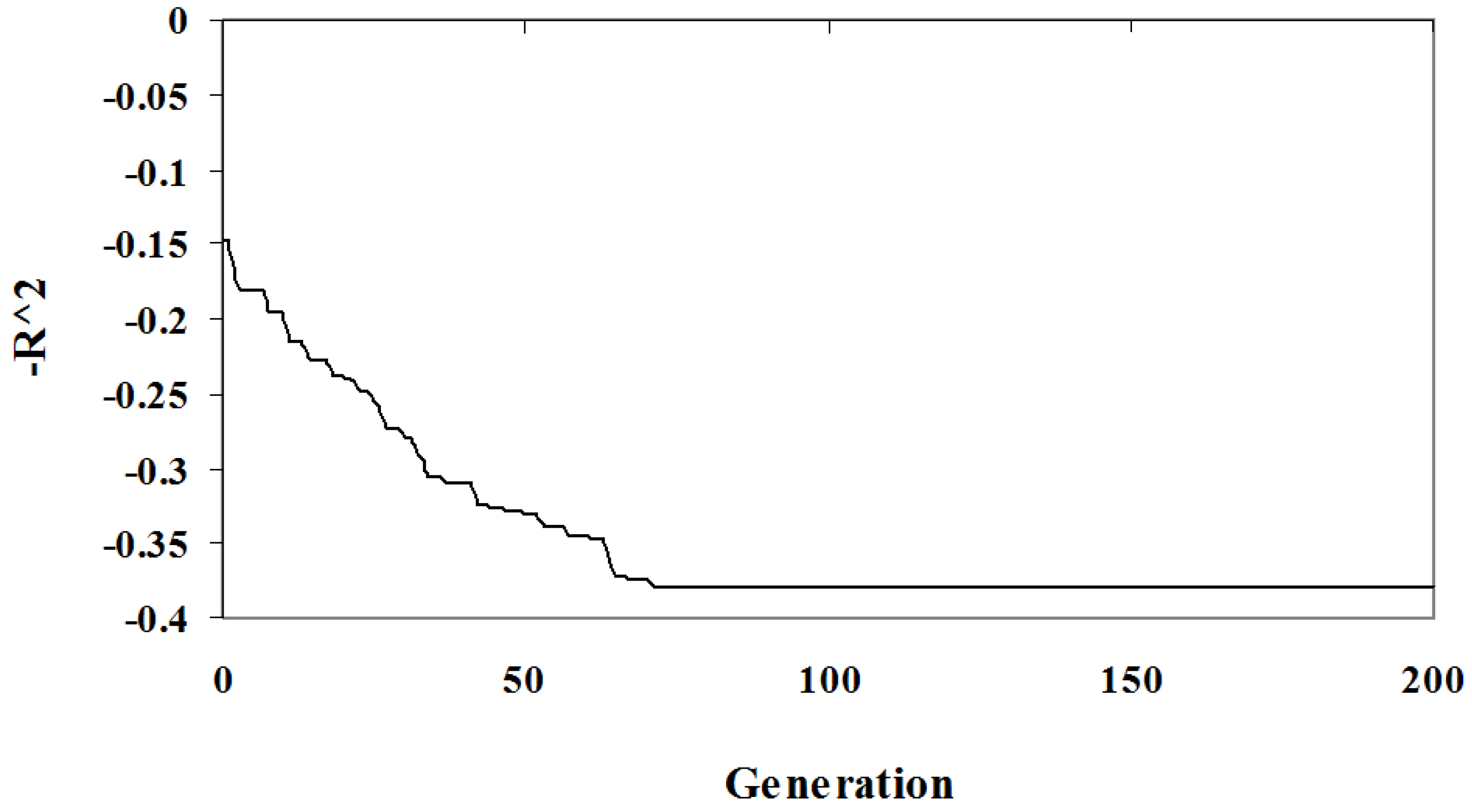
The relationship between solution quality and algorithm iteration is depicted in Figure 1 and Figure 2. The graphs show the best solution at each step in an arbitrary randomized simulation. Initially, the population has a low quality fit and a high complexity since it is random. As the algorithm progresses the optimization criteria improves and the best solution eventually reaches a local minima and so will be included in the Pareto optimal set. In Figure 1 and Figure 2 the solution identified has a complexity of three parameters (out of the seven), the $R^2$ fit is low at $0.38$. This example demonstrates the diversity of solutions found; some of these solutions under-fit the problem at the expense of accuracy.

Figure 1. Algorithm Sample Run: The $-R^2$ value as a function of algorithm iteration of the best individual for an arbitrary simulation.

Figure 1. Algorithm Sample Run: The $-R^2$ value as a function of algorithm iteration of the best individual for an arbitrary simulation.

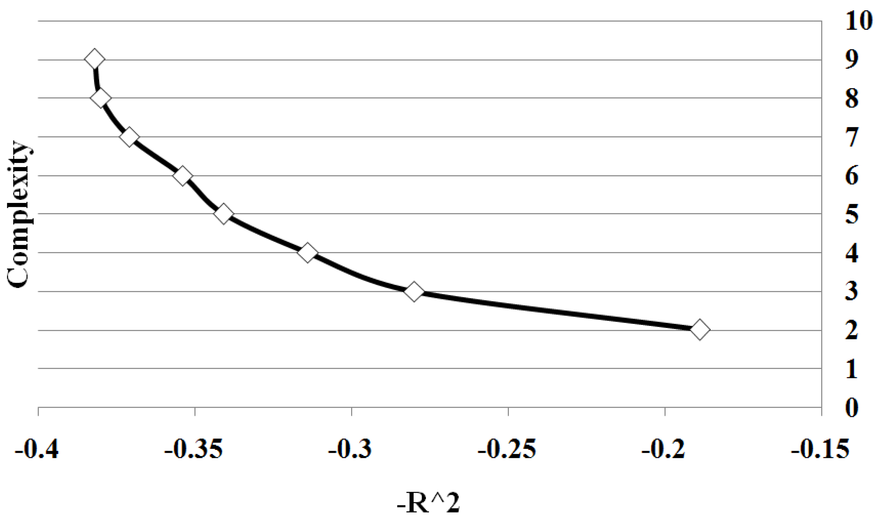
Figure 3 shows all points on Pareto front between solution complexity 2 and 10. We summarize the results of the different sample sizes by averaging the goodness of fit for each solution complexity. Note the classic trade-off is illustrated between complexity and accuracy. As the complexity increases, the goodness of fit tends to increase. Significantly there is a change in the form of the trade-off curve at the point when the complexity of the solution exactly matches the known complexity of the given problem. Note how once the solution begins to over-fit the correct solution, the improvement in goodness of fit diminishes with the increase in complexity. By determining the maximum rate of change of goodness of fit with respect to the complexity, the optimal complexity could be identified that minimizes over and under fitting.

Figure 2. Algorithm Sample Run: The complexity as a function of algorithm iteration of the best individual for an arbitrary simulation.

Figure 2. Algorithm Sample Run: The complexity as a function of algorithm iteration of the best individual for an arbitrary simulation.

Figure 3. Case I Pareto Front: showing the relation between $-R^2$ and complexity for Case 1. The values are average of 10 runs of 100 simulation replicates.

Figure 3. Case I Pareto Front: showing the relation between $-R^2$ and complexity for Case 1. The values are average of 10 runs of 100 simulation replicates.

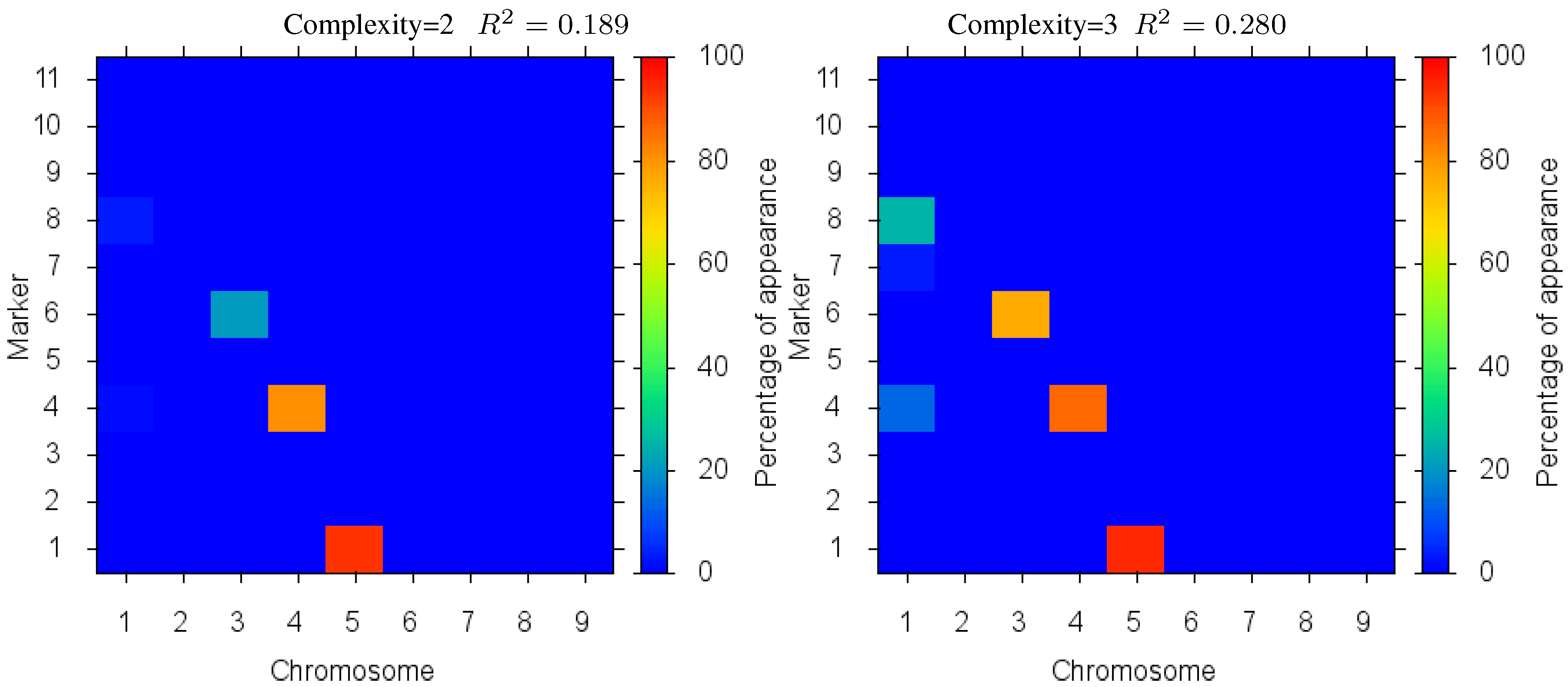
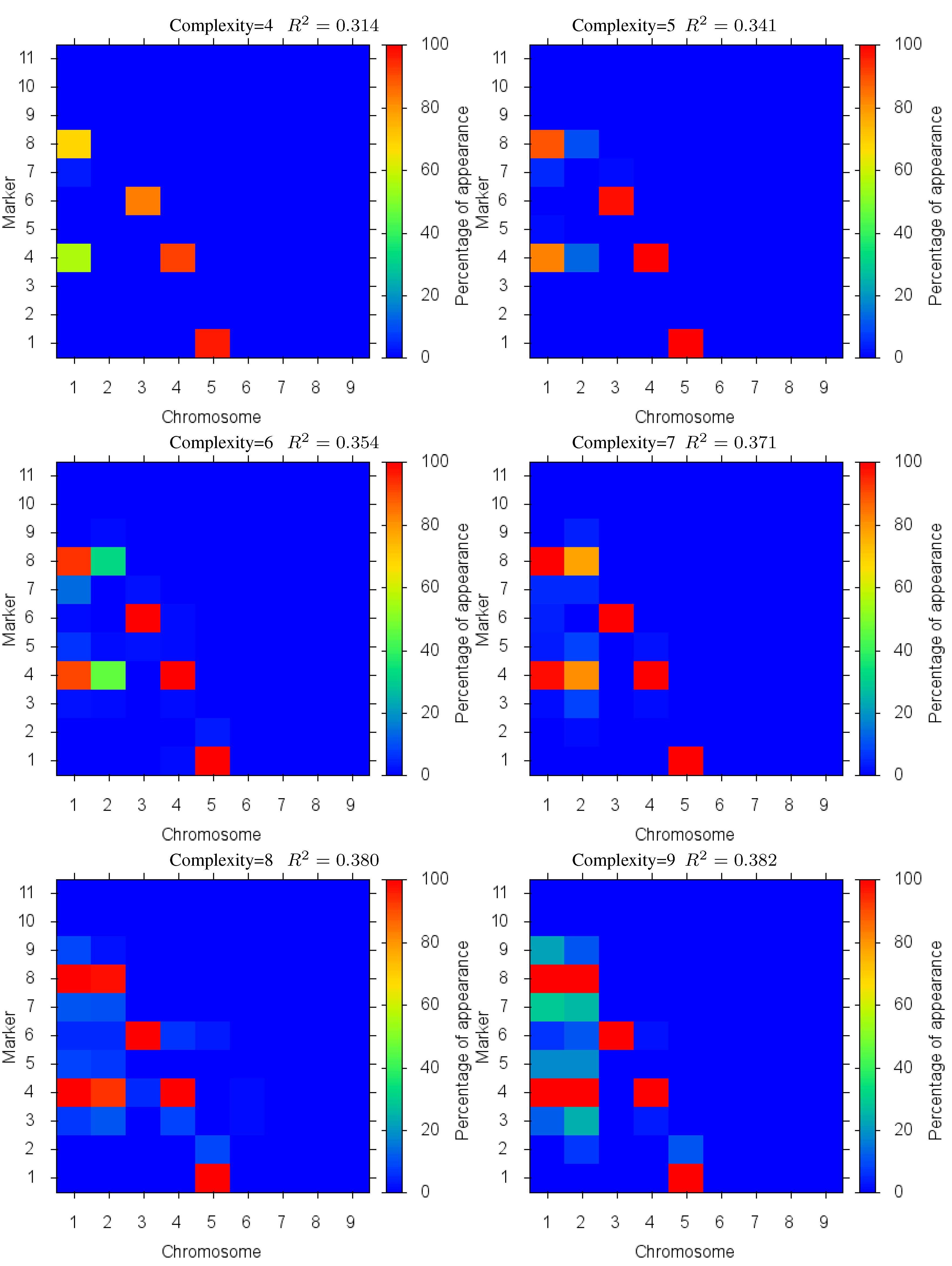
Figure 4 shows the markers identified for each solution complexity, with each figure the sum over the randomized program runs. Since a red marker means maximal identification, the solution with complexity 7 consistently finds the correct location of all 7 markers, while avoiding extraneous markers. Interestingly, the synergistically linked markers are consistently identified, irrespective of solution complexity. Solutions with complexity 3 through 5 find the five correct synergistic markers. QTLs that were coupled antagonistically (chromosome 2, position 4 and 8) proved much more difficult to identify. A low proportion of runs with complexity 6 find these markers, increasing in proportion as solution complexity grows. However, when complexity exceeds the given 7 parameters, many nearby extraneous markers begin to be found.

Figure 4. Case I Identified Markers: Identified markers found in different complexity Pareto optimal solutions for Case I. The color is the proportion of random executions that the specific marker was found. Bright red signifies that in each run the marker was consistently found. Blue means that the marker did not appear in any solutions.

Figure 4. Case I Identified Markers: Identified markers found in different complexity Pareto optimal solutions for Case I. The color is the proportion of random executions that the specific marker was found. Bright red signifies that in each run the marker was consistently found. Blue means that the marker did not appear in any solutions.

To validate and compare the performance of this approach, we used Windows QTL Cartographer (WQTLC) Ver. 2.5 [36] that uses a Bayesian Interval Mapping approach. The comparative results are shown in Table 2. The results show that MOEA method improves the performance in every category. Identification of correct markers is consistently better than Cartographer, with the best improvement for smaller data sets. Also the MOEA approach has lower rate of detection of extraneous linked QTL and does not predict extraneous unlinked QTLs. We performed the two-sample Kolmogorov-Smirnov test to compare the results obtained by our MOEA method against the WQTLC results. This test quantifies the distance between two results sets and analyzes the null hypothesis that the two sets are from the same distribution. This test was performed for all corresponding data elements in Table 2; using 1% and 5% significance levels, the null hypothesis was rejected for all the tests.

Table 2. Case I: MOEA vs. Bayesian Interval Mapping: Comparative results of the MOEA approach vs. Bayesian Interval Mapping method using Windows QTL Cartographer version 2.5 with complexity of 7. The number in the tables is the average of the count of parameters found. So the best result for the Correct column would be 7.0. Ex-L is the number of extraneous linked QTL and Ex-UL is the number of extraneous unlinked QTLs. The best result for these columns would be 0.0.

DataSet Size	Bayesian Interval Mapping			MOEA Method
	Correct	Ex-L	Ex-UL	Correct	Ex-L	Ex-UL
100	2.16 ± 1.06	0.82 ± 0.44	0.41 ± 0.37	4.54 ± 1.77	1.08 ± 0.52	0.08 ± 0.05
200	5.21 ± 0.80	0.36 ± 0.15	0.15 ± 0.12	6.77 ± 0.93	0.21 ± 0.17	0.0 ± 0.0
300	6.69 ± 0.28	0.33 ± 0.24	0.02 ± 0.02	6.92 ± 0.11	0.06 ± 0.06	0.0 ± 0.0

Table 2. Case I: MOEA vs. Bayesian Interval Mapping: Comparative results of the MOEA approach vs. Bayesian Interval Mapping method using Windows QTL Cartographer version 2.5 with complexity of 7. The number in the tables is the average of the count of parameters found. So the best result for the Correct column would be 7.0. Ex-L is the number of extraneous linked QTL and Ex-UL is the number of extraneous unlinked QTLs. The best result for these columns would be 0.0.

DataSet Size	Bayesian Interval Mapping			MOEA Method
	Correct	Ex-L	Ex-UL	Correct	Ex-L	Ex-UL
100	2.16 ± 1.06	0.82 ± 0.44	0.41 ± 0.37	4.54 ± 1.77	1.08 ± 0.52	0.08 ± 0.05
200	5.21 ± 0.80	0.36 ± 0.15	0.15 ± 0.12	6.77 ± 0.93	0.21 ± 0.17	0.0 ± 0.0
300	6.69 ± 0.28	0.33 ± 0.24	0.02 ± 0.02	6.92 ± 0.11	0.06 ± 0.06	0.0 ± 0.0

4.2. Experiment Case II

For the second test case we considered a model with seven QTLs with increasing effect, 0.5, 0.55, 0.6, 0.65, 0.7, 0.75 and 0.8 at the same locations as the first test case. In this test we intended to show the power of the algorithm in detecting the QTLs ordered by their effect on the phenotype output. The Pareto front is depicted in Figure 5 and detailed results are shown in Figure 6. As results show, each marker’s magnitude tends to be more consistently detected and be included in the simpler solutions, signalled by the deeper red color. The only exception is for makers on chromosome 2 that are linked antagonistically. Here, antagonistic markers are consistently detected only in solutions whose complexity is near or equal to the problem complexity. As in Case I, as solution complexity increases beyond the given problem size, there is an increase of nearby extraneous parameters, but little increase in accuracy. We performed the Kolmogorov-Smirnov test for the results of this experiment too. Like in the first experiment, the null hypothesis was rejected for all the tests under 1% and 5% significance levels.

Figure 5. Case II Pareto Front: Pareto front showing the relation between $-R^2$ and complexity for Case II. The values are average of 10 runs of 100 simulation replicates.

Figure 5. Case II Pareto Front: Pareto front showing the relation between $-R^2$ and complexity for Case II. The values are average of 10 runs of 100 simulation replicates.

Figure 6. Case II Markers Identified: in different complexity Pareto optimal solutions for Case II. The color is the proportion of random executions that the specific marker was found. Bright red signifies that in each run the marker was consistently found. Blue means that the marker did not appear in any solutions.

Figure 6. Case II Markers Identified: in different complexity Pareto optimal solutions for Case II. The color is the proportion of random executions that the specific marker was found. Bright red signifies that in each run the marker was consistently found. Blue means that the marker did not appear in any solutions.

As results in Table 3 show, the detection accuracy of case II is decreased compared to Case I; the reason for this is the difficulty of detection of markers with small effect of QTLs on the trait. Again, in this experiment the performance of the MOEA method is consistently better than WQTLC over all evaluation criteria. The best improvement is demonstrated with smaller data sets, a more likely case in real experiments. When the sample size is small, the MOEA method identified on average about one near-by extraneous linked QTLs, which can still be of value to scientists when the correct linked QTLs are weakly detected.

Table 3. Case II: MOEA vs. Bayesian Interval Mapping: Comparative results of the MOEA approach vs. Bayesian Interval Mapping method using Windows QTL Cartographer version 2.5 with complexity of 7.

DataSet Size	Bayesian Interval Mapping			MOEA Method
	Correct	Ex-L	Ex-UL	Correct	Ex-L	Ex-UL
100	2.65 ± 0.99	1.23 ± 0.84	0.29 ± 0.22	4.06 ± 0.75	1.15 ± 0.40	0.11 ± 0.10
200	4.90 ± 1.24	0.70 ± 0.63	0.13 ± 0.15	6.26 ± 0.81	0.44 ± 0.33	0.03 ± 0.06
300	6.36 ± 0.30	0.29 ± 0.16	0.07 ± 0.10	6.84 ± 0.18	0.17 ± 0.09	0.0 ± 0.0

Table 3. Case II: MOEA vs. Bayesian Interval Mapping: Comparative results of the MOEA approach vs. Bayesian Interval Mapping method using Windows QTL Cartographer version 2.5 with complexity of 7.

DataSet Size	Bayesian Interval Mapping			MOEA Method
	Correct	Ex-L	Ex-UL	Correct	Ex-L	Ex-UL
100	2.65 ± 0.99	1.23 ± 0.84	0.29 ± 0.22	4.06 ± 0.75	1.15 ± 0.40	0.11 ± 0.10
200	4.90 ± 1.24	0.70 ± 0.63	0.13 ± 0.15	6.26 ± 0.81	0.44 ± 0.33	0.03 ± 0.06
300	6.36 ± 0.30	0.29 ± 0.16	0.07 ± 0.10	6.84 ± 0.18	0.17 ± 0.09	0.0 ± 0.0

4.3. Experiment Case III

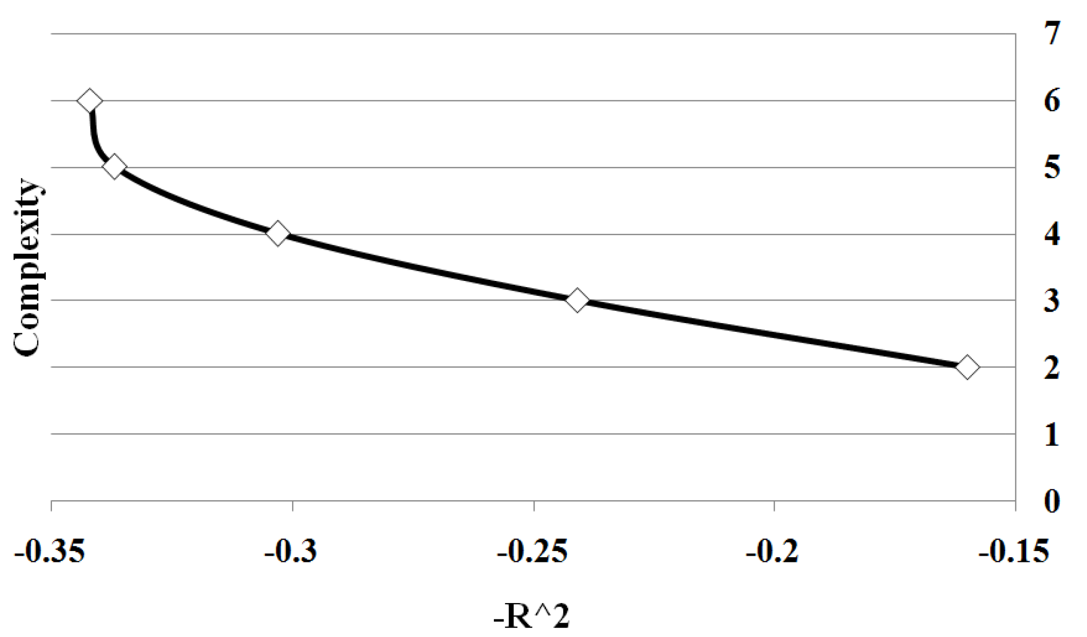
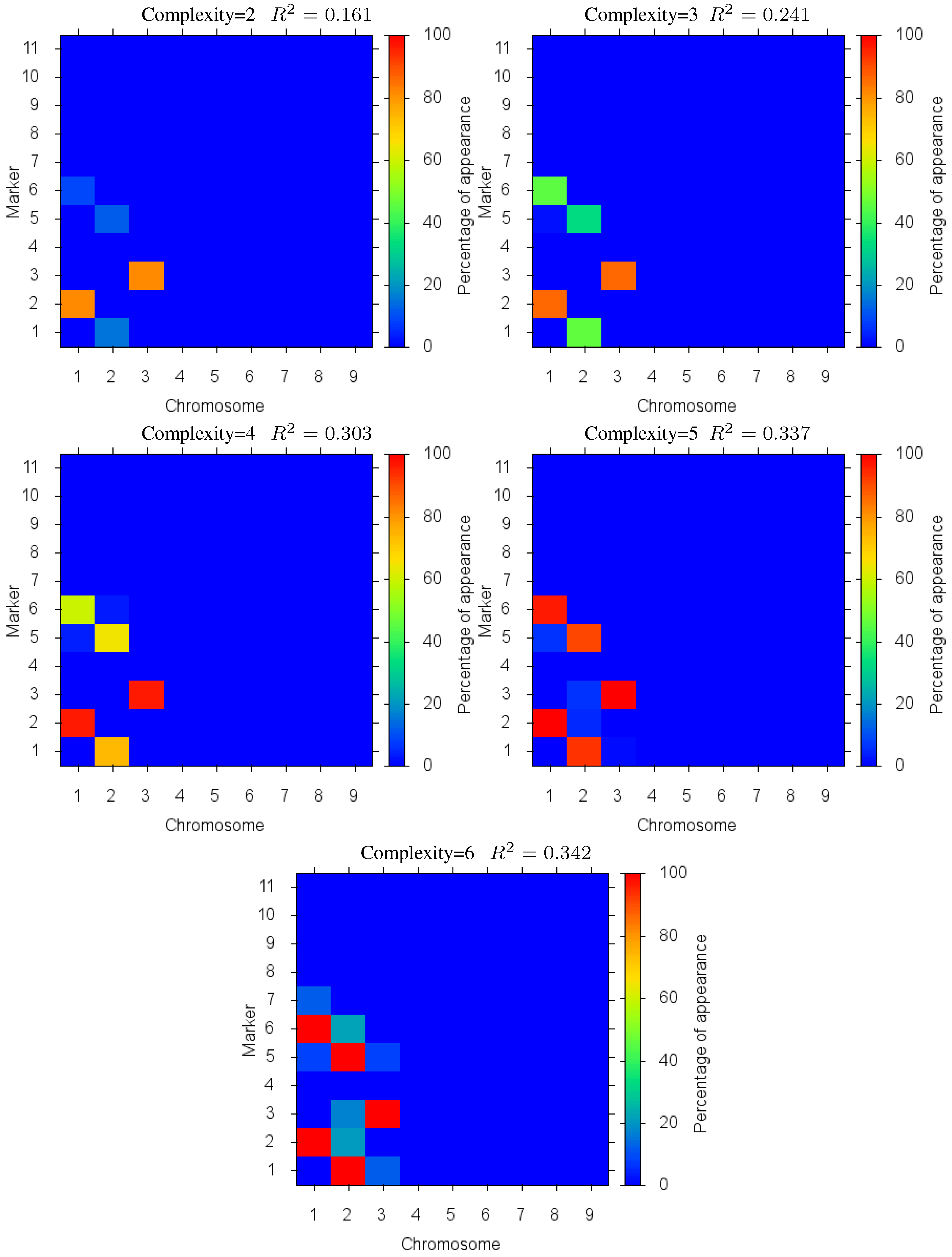
This test case introduces the complexity of epistatic interactions and therefore the challenge of finding the coupled parameters in a much enlarged search space. In this case, the epistatic interactions are introduced by a model with 4 chromosomes each 70 cM long and with 8 markers located at a distance of 10 cM. Like previous test cases QTLs are positioned exactly at marker loci; we modeled 3 QTLs with effect 0.7: marker 6 on chromosome 1, markers 1 and 5 on chromosome 2. We also considered an epistatic interaction between 2 QTLs with effect 0 independently, but in combination they will have effect 0.8: marker 2 on chromosome 1 and marker 3 on chromosome 3. There is no QTL on chromosome 4.

The Pareto front for this test case is depicted in Figure 7. In this case, we see the same effect as before where the increase in quality of fit diminishes as over fitting occurs (beyond complexity 5). Detailed marker identification results are illustrated in Figure 8 showing the percentage of markers found. Since the epistatic interaction has the highest effect on the trait it is detected more than the other loci at low complexities, signalled by the two loci in the epistatic interaction being identified together with a high percentage. These results demonstrate the effectiveness of the method in identifying biologically significant coupled gene interactions.

Figure 7. Case II Pareto Front: showing the relation between $-R^2$ and complexity for Case III. The values are average of 10 runs of 100 simulation replicates.

Figure 7. Case II Pareto Front: showing the relation between $-R^2$ and complexity for Case III. The values are average of 10 runs of 100 simulation replicates.

A comparison of the method with Bayesian Interval Mapping of Windows QTL Cartographer was not performed due to inability of the WQTLC tool to detect epistatic loci interactions.

Figure 8. Case III: Markers Identified: in different complexity Pareto optimal solutions for Case III. The color is the proportion of random executions that the specific marker was found. Bright red signifies that in each run the marker was consistently found. Blue means that the marker did not appear in any solutions.

Figure 8. Case III: Markers Identified: in different complexity Pareto optimal solutions for Case III. The color is the proportion of random executions that the specific marker was found. Bright red signifies that in each run the marker was consistently found. Blue means that the marker did not appear in any solutions.

5. Conclusions

We developed an extinction-based multi-objective evolutionary approach to solve QTL mapping problem. The Genetic Algorithm searches the powerset of marker pairs along with the powerset of individual markers in order to identify both additive and epistatic genes that control a quantitative trait. Effectively searching such a large space and identifying biologically relevant results is challenging for many reasons. First, there is a need to avoid the premature convergence to local minima solutions by the GA. In this work the method of population extinction is used to ensure continued population diversity. Second, in order to obtain solutions that can be of use for biologists and truly represent the underlying genetic mechanisms, parsimonious solutions must be found. Here, another minimization objective is introduced into the search that measures the number of parameters of solutions, and multi-objective optimization performed. Third, the search engine must not only identify the markers that contribute to the quantitative trait, but also their magnitude and whether they have negative or positive influence. To solve this problem and identify the parameter values, the search engine applies PLS to fit the best predictive function over only those markers in each potential GA solution.

Using the methodology from [35] experiments were performed demonstrating the effectiveness of the new method in solving realistic QTL problem instances with hundreds of samples and complex gene interactions. In each case the results obtained were compared with results from the Bayesian Interval Mapping method using Windows QTL Cartographer (WQTLC) Ver. 2.5 [36]. The GA algorithm consistently identified additional correct marker locations which were missed by the Bayesian Interval Mapping approach even when the data set was relatively large. The problem of false positives where markers that do not exist in the problem are identified incorrectly is minimized in the new approach. Unlinked markers that exist away from the correct markers were never found once the data set exceeded 100 samples. Linked markers that lie nearby were still incorrectly identified, but at a lower rate than the Bayesian Interval Mapping approach employed by WQTLC. These errors are of less consequence since they can still provide useful information to the scientists.

Significantly, exploring the trade off between model complexity and accuracy using the multi-optimization approach provides insights into the QTL problem not available in many other approaches. Having the Pareto optimal frontier available to the scientists studying the QTL data enables them to select the solution that best matches their biological objective. As discussed in the results, solutions that under-fit the data often identify the most influential markers for the trait and point the scientists to those genes whose modification could produce the most benefit for the least cost. Additionally, the most accurate solution complexity (between over and under fitting the data) is apparent from the Pareto optimal frontier by observing the point where increases in solution complexity lead to insignificant improvements in accuracy.

An important and almost universal problem in modeling biological data is selecting the true features from the multitude of irrelevant features masking the desired model. This work presents a hybrid approach to solving this problem where a GA searching the powerset of features is combined with a statistical approach that measures the significance and utility of each generated feature set.