Extracting Co-Occurrence Relations from ZDDs

Abstract

A zero-suppressed binary decision diagram (ZDD) is a graph representation suitable for handling sparse set families. Given a ZDD representing a set family, we present an efficient algorithm to discover a hidden structure, called a co-occurrence relation, on the ground set. This computation can be done in time complexity that is related not to the number of sets, but to some feature values of the ZDD. We furthermore introduce a conditional co-occurrence relation and present an extraction algorithm, which enables us to discover further structural information.

1. Introduction

Enumerating a large number of sets and finding useful information from them have recently attracted the attention of many researchers. The data structure called a zero-suppressed binary decision diagram [1], ZDD for short, is known to be useful for compactly representing collections of sets and for efficiently manipulating them. ZDDs have been applied to various problems. In the analysis of transaction databases, Minato and Arimura [2,3] invented ZDD-based techniques for frequent itemset mining. Coudert [4] introduced a ZDD-based approach to solve many graph and set optimization problems. Sekine and Imai [5] developed a new paradigm of the exact computation for network reliability by means of binary decision diagrams (see [6,7]), BDDs for short. Recently, for multi-terminal binary decision diagrams, which are a well accepted technique for the state graph based quantitative analysis of large and complex systems, a zero-suppressed version has been studied by Lampka et al. [8]. Roughly speaking, an idea common to these is to compress a large number of sets into a ZDD (BDD) and manipulate them without decompression.

In this paper, we study the following basic problem of ZDDs: Given a ZDD representing a set family, extract a hidden structure, called a co-occurrence relation, over the ground set. This computation can be done in time complexity that is related not to the number of sets, but to some feature values of the ZDD representing the sets. Thus it is effective especially when a large number of sets are compressed into a small ZDD. Since we do not put any domain-specific assumption on the sets represented by a ZDD, our algorithm is widely applicable to ZDDs obtained from real-life data.

The co-occurrence relation is defined as follows: given a set S and a collection C of subsets of S, two elements $a,b\in S$ co-occur with each other for C if it holds that for all $T\in C$, $a\in T$ if and only if $b\in T$. In a series of work for finding various useful information from databases [9,10,11], the co-occurrence relation was introduced, although an efficient extraction algorithm is not known. Clearly the co-occurrence relation is an equivalence relation and it induces the partition consisting of equivalence classes, called a co-occurrence partition. Since ZDDs represent collections of sets, co-occurrence relations and partitions are similarly defined for ZDDs. Since elements in the same block of a co-occurrence partition have the same behavior, when we want to find useful information from a ZDD, we need not distinguish between them and the ZDD can be compressed further.

This paper is organized as follows. In Section 2 we introduce some basic notions on ZDDs. We present algorithms in Section 3 and provide examples in Section 4. Concluding remarks are given in Section 5.

2. Basic Notions on ZDDs

Since we do not treat BDDs, we only introduce ZDDs. ZDDs are graph representations for set families. Figure 1(b) illustrates the ZDD representing the set family $\{\varnothing ,\left\{e_1\right\},\left\{e_2\right\},\left\{e_3\right\}\}$. Whenever a ZDD is given, we always assume that a ground set S and the order of the elements are fixed. For simplicity, let $S:=\{e_1,\dots ,e_n\}$, where the elements are numbered from 1 to $n(=|S\left|\right)$ and ordered in this order. The node at the top is called the root. Each internal node has the three fields V, LO and HI. The field V holds the index of an element in S. The fields LO and HI point to other nodes, which are called LO and HI children, respectively. The arc to a LO child is called a LO arc and illustrated by a dashed arrow, while the arc to a HI child is called a HI arc and illustrated by a solid arrow. There are only two non-internal nodes, denoted by ⊥ and ⊤.

Figure 1. The two graph representations for the same set family $\{\varnothing ,\left\{e_1\right\},\left\{e_2\right\},\left\{e_3\right\}\}$. (a) Binary Decision Tree; (b) ZDD.

Figure 1. The two graph representations for the same set family $\{\varnothing ,\left\{e_1\right\},\left\{e_2\right\},\left\{e_3\right\}\}$. (a) Binary Decision Tree; (b) ZDD.

The following two conditions for ZDDs enable a unique and efficient representation. First, whenever an arc goes from an internal node f to an internal node g, a ZDD must satisfy $\mathrm{V}\left(f\right)<\mathrm{V}\left(g\right)$. Thus no nodes having the same index occur twice in a path. Second, a ZDD must be irreducible in the sense that the following reduction operations cannot be applied anymore.

• For each internal node f whose HI child is ⊥, redirect all the incoming arcs of f to the LO child of f, and then eliminate f (Figure 2(a)).
• Share all equivalent subgraphs (Figure 2(b)).

Figure 2. The two reduction rules for ZDDs. (a) Node Elimination; (b) Node Sharing.

Figure 2. The two reduction rules for ZDDs. (a) Node Elimination; (b) Node Sharing.

Now, let us see the correspondence between ZDDs and set families. Given a ZDD, for each path P from the root to ⊤, define a subset $T_P$ of S such that $e_i\in T_P$ if the HI arc of an internal node f is selected (where $i=\mathrm{V}\left(f\right)$); otherwise, $e_i\notin T_P$. Note that if P contains no nodes of index i, then we can know that $e_i\notin T_P$ due to the node elimination rule. We obtain the set family $\left\{T_P:P\text{is}\text{a}\text{path}\text{in}\text{the}\text{ZDD}\right\}$. Conversely, given a set family, construct the corresponding binary decision tree as is illustrated in Figure 1(a) and make it irreducible by applying the two reduction rules. Observe for example that Figure 1(b) is obtained from Figure 1(a). It is known (see [1,12] (§7.1.4), for details) that every set family has one and only one representation as a ZDD if the size of a ground set and the order of the elements are fixed.

For any node f in a ZDD, the graph consisting of all nodes accessible from f forms a ZDD whose root is f. The size of a ZDD is the total number of nodes in the ZDD, including non-internal nodes. The cardinality of a node is the total number of paths from the node to ⊤. Since in ZDDs we are interested in paths leading to ⊤, we mean by a branch node an internal node whose two children have paths leading to ⊤; in other words, the LO child is not ⊥. Note that a branch node is not a synonym of an internal node.

3. Algorithms

We present an algorithm to extract a hidden structure, called a co-occurrence relation, from a ZDD. Our algorithm constructs a co-occurrence partition while traversing a ZDD. We first explain how to traverse a ZDD and then how to manipulate a partition efficiently in the traversal. We furthermore introduce the notion of a conditional co-occurrence relation and present an extraction algorithm.

3.1. Traversal Part

Let us first consider a naive method to compute a co-occurrence partition. Suppose that a ZDD represents a collection C of subsets of a set S. The co-occurrence partition is incrementally constructed as follows. We start with the partition $\left\{S\right\}$ consisting of the single block S. For each path P from the root to ⊤, we obtain a new partition from the current partition by separating each block b into the two parts $b\cap T_P$ and $b\cap (S\setminus T_P)$ if both parts are nonempty, where $T_P$ denotes the set in C corresponding to P. 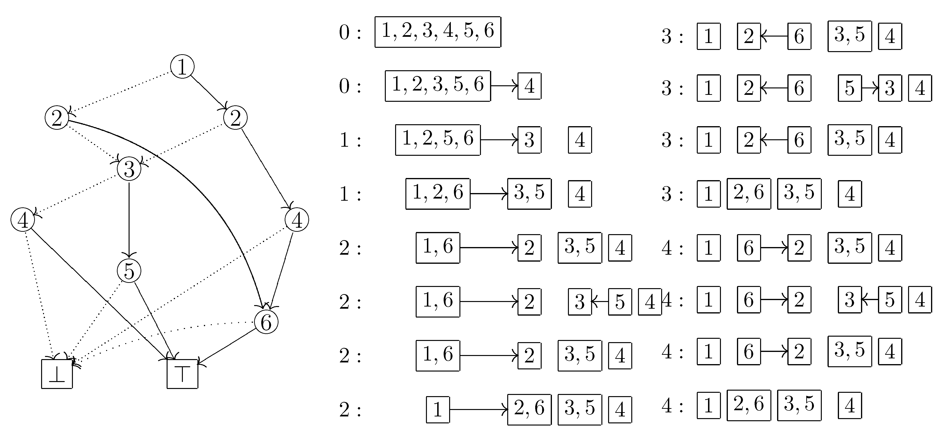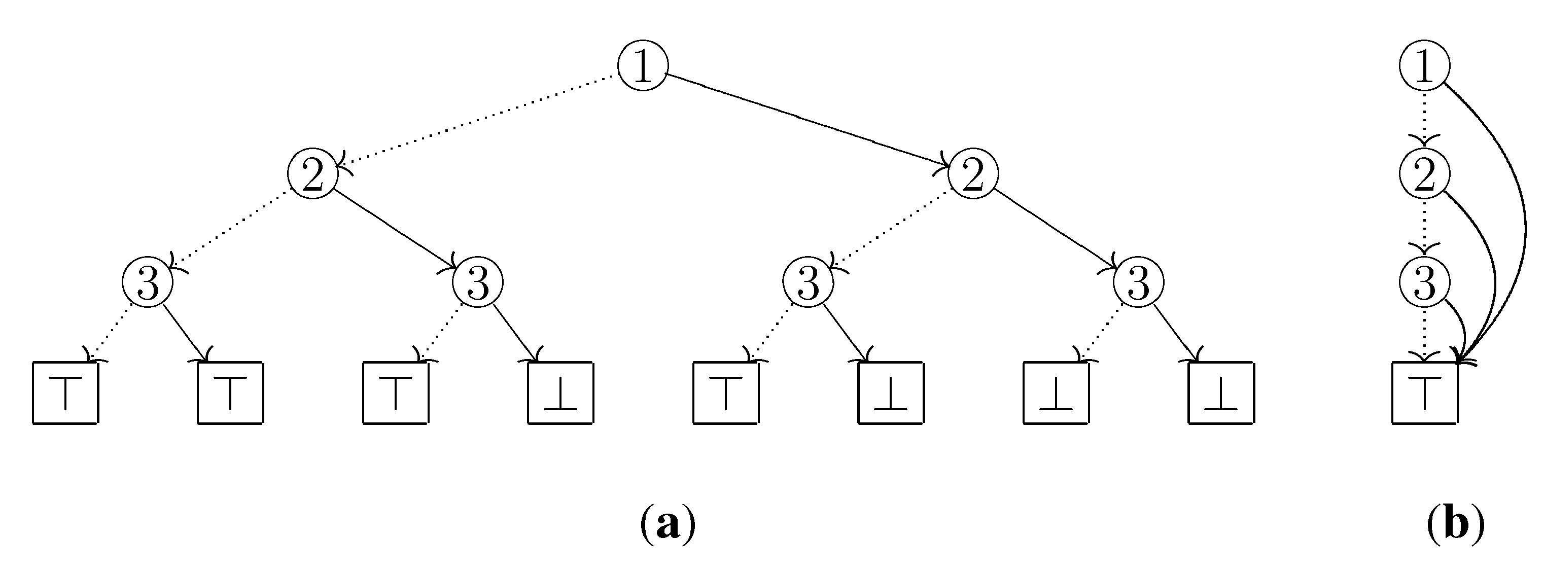This can be done by checking which arc is selected at each node of P. For example, let us see the ZDD given in Figure 3: If we first examine the path $1⤏2⤏3⤏4\to \top$, then the block S of the initial partition splits into the two parts $\left\{4\right\}$ and $S\setminus \left\{4\right\}$, since HI arc is selected only at the label 4 node. It can be easily verified that after all paths are examined, the co-occurrence partition induced by C is constructed. However, since this method depends on the number of paths (thus the size of C), this is not effective for ZDDs which efficiently compress a large number of sets. It would be desirable if we could construct a co-occurrence partition directly from a ZDD.

Figure 3. The computing process of our algorithm for the ZDD that represents the set family $\{\left\{e_4\right\},\{e_3,e_5\},\{e_2,e_6\},\{e_1,e_4\},\{e_1,e_3,e_5\},\{e_1,e_2,e_4,e_6\}\}$ is shown below. For example, in the third line from the bottom of the left column, the number 2 on the left side means that ⊤ was visited twice; the right arrow means that the state of $e_2$ changed from LO to HI; the left arrow means that the state of $e_3$ changed from HI to LO. In the bottom of the right column, the co-occurrence partition $\{\left\{e_1\right\},\{e_2,e_6\},\{e_3,e_5\},\left\{e_4\right\}\}$ is obtained.

Figure 3. The computing process of our algorithm for the ZDD that represents the set family $\{\left\{e_4\right\},\{e_3,e_5\},\{e_2,e_6\},\{e_1,e_4\},\{e_1,e_3,e_5\},\{e_1,e_2,e_4,e_6\}\}$ is shown below. For example, in the third line from the bottom of the left column, the number 2 on the left side means that ⊤ was visited twice; the right arrow means that the state of $e_2$ changed from LO to HI; the left arrow means that the state of $e_3$ changed from HI to LO. In the bottom of the right column, the co-occurrence partition $\{\left\{e_1\right\},\{e_2,e_6\},\{e_3,e_5\},\left\{e_4\right\}\}$ is obtained.

Our algorithm improves the naive method above by avoiding as many useless visits of nodes as possible. We traverse a ZDD basically in a depth-first order. In each node, we select the next node in a LO arc first order, i.e., the LO child if the LO child is not ⊥; otherwise, the HI child. After we arrive at ⊤, we go back to the most recent branch node and select the HI arc. Note that we need not go back to the root, since arc types do not change until the most recent branch node. For example, in Figure 3, after the first visit of ⊤, we go back to the label 3 node and go ahead along the path $3\to 5\to \top$.

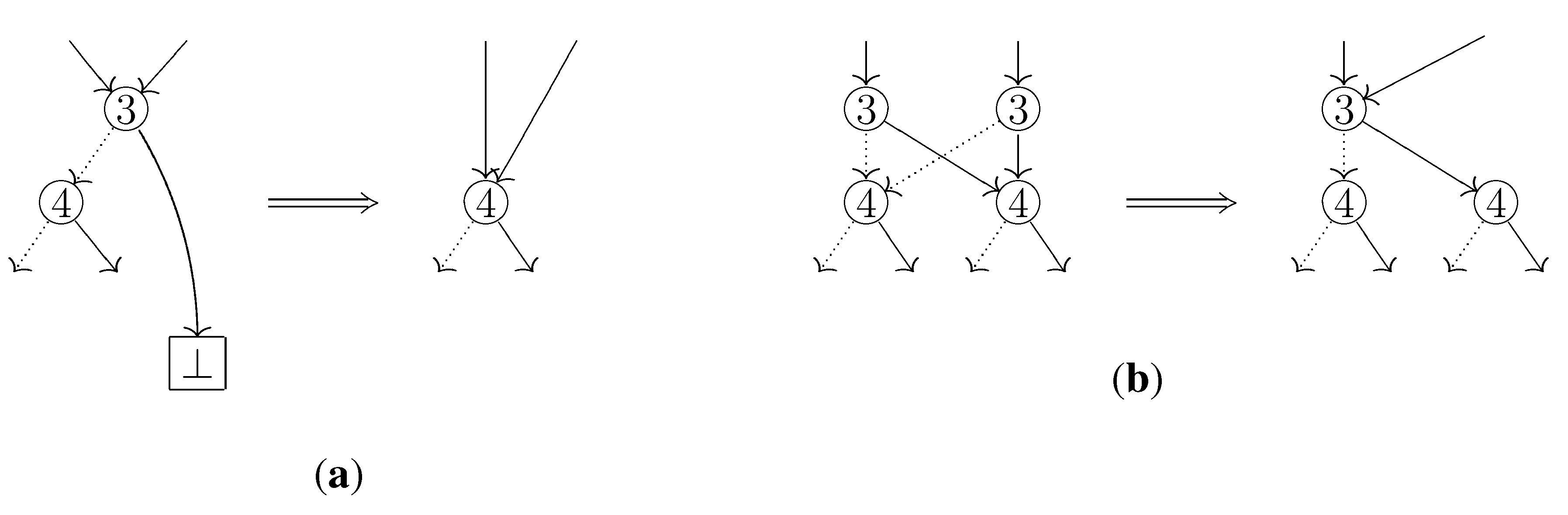
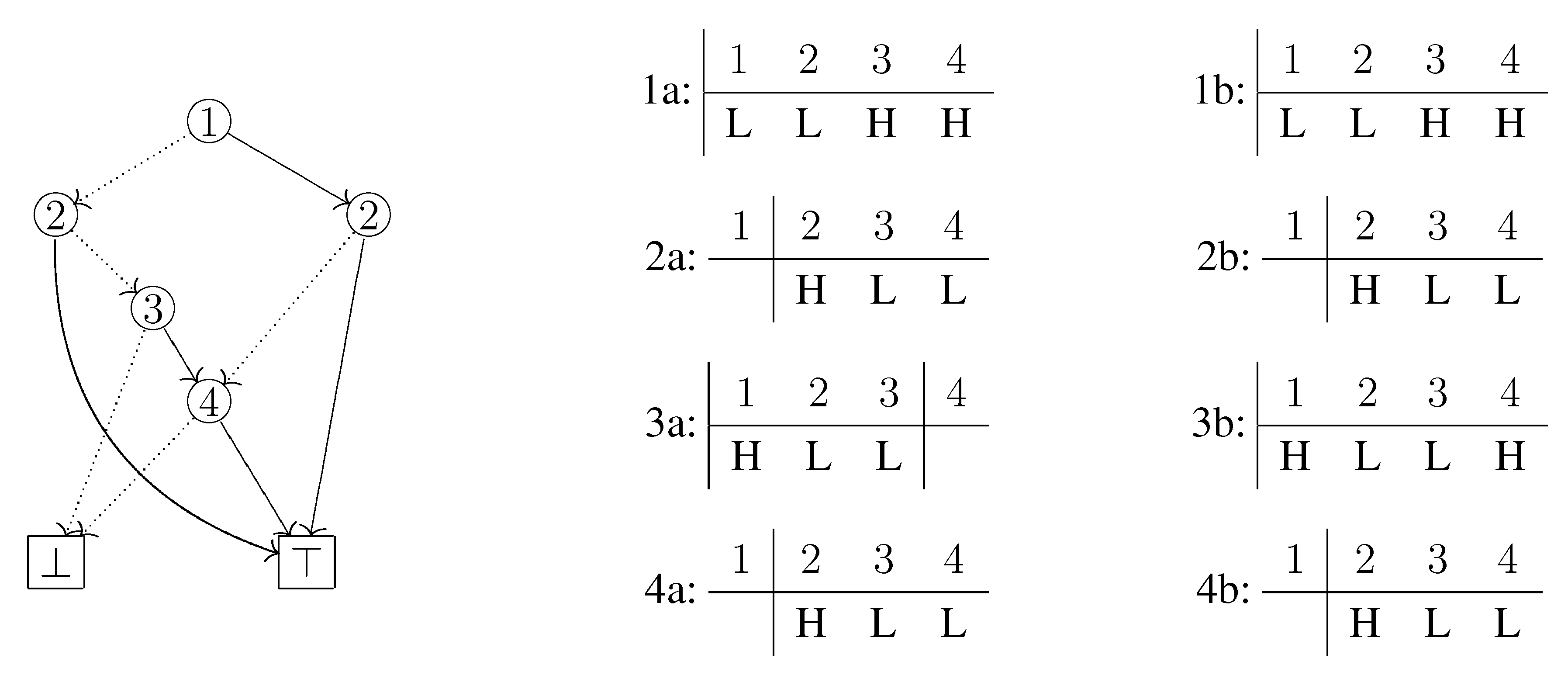
The difference from the usual depth-first search is that when we visit an already visited node, we go down from the node to ⊤ by selecting only HI-arcs. This is essential because the usual depth-first search may fail to detect separable elements. For example, in Figure 4, the two elements $e_3$ and $e_4$ are separable, and in our traversal the third and fourth columns in the table 3b have different arc types thus we can know that they are really separated. On the other hand, in the usual depth-first search they are observed as if they had a common arc type: Since an already visited node is no longer visited, the arc type of $e_4$ in the table 3a is not updated, which means the type remains LO.

Figure 4. Each table on the center shows the change of selected arc types when the ZDD is traversed by the usual depth-first search. Similarly, the tables on the right correspond to the changes when traversed by our algorithm.

Figure 4. Each table on the center shows the change of selected arc types when the ZDD is traversed by the usual depth-first search. Similarly, the tables on the right correspond to the changes when traversed by our algorithm.

Unlike the usual depth-first search, we do not skip necessary paths as the following lemma implies.

Lemma 3.1. In each visit of a node g after the first, two elements get separated when traversing the subgraph whose root is g if and only if they get separated when going from g to ⊤ with only HI-arcs.

Proof. Since the sufficiency is immediate, we only show the necessity. Suppose for contradiction that two elements $e_i$ and $e_j(i<j)$ get separated when visiting all nodes below g, while they are not separated when only selecting HI-arcs. Let $e_k$ denote the element corresponding to g. For the case $i<k$, there are two paths from g such that they have different arc types at $e_j$. However, in the first visit of g, we could trace both paths and know that $e_i$ and $e_j$ are separated, which is a contradiction. For the other case $k\le i$, there is a path from g with different arc types at $e_i$ and $e_j$, and we could trace this path in the first visit of g and reach a contradiction.

The traversal part is formally described in Algorithm 1. We here explain some notation and terminology. Recall that in each internal node f, the next node of f in a LO arc first order is the LO child if f is a branch node, i.e., an internal node whose two children have paths leading to ⊤; otherwise, the HI child. In order to traverse a ZDD, branch nodes are pushed onto the stack BRANCH, and visited nodes are contained in $N_{\text{visited}}$. The ⊤ is contained in $N_{\text{visited}}$ in the initialization part, which reduces an exceptional case in the traversal part, i.e., the loop block. For each step of the traversal, by invoking the function Update, we update the current partition p according to which arc is selected at the currently visited node f and whether there exist nodes hidden between f and the next node g due to the node elimination rule. To do this efficiently, we need the following things: The graph structure G defined on the blocks of p, the set $B_{\text{new}}$ of blocks which have been created since the last visit of ⊤, and the set $E_{\text{HI}}$ of elements whose arc types are HI. The set $B_{\text{new}}$ is refreshed for each visit of ⊤. The function Update is explained in detail in the next subsection.

Algorithm 1 Calculate a co-occurrence partition from a ZDD defined on a set $S:=\{e_1,\dots ,e_n\}$

Require: ZDD is neither ⊥ nor ⊤, and $n>0$   $p\leftarrow$ the partition $\left\{S\right\}$;   $G\leftarrow$ the digraph with no arc and one vertex corresponding to the unique block S of p;   $E_{\text{HI}}\leftarrow \varnothing$; $B_{\text{new}}\leftarrow \varnothing$; Initialize BRANCH as an empty stack;   $f\leftarrow$ the root of ZDD;   $g\leftarrow$ the next node of f in a LO arc first order;   $N_{\text{visited}}\leftarrow \{\top ,f\}$;   if f is a branch node then       push f onto BRANCH;   end if   loop       $\text{Update}\left(f,g,p,G,B_{\text{new}},E_{\text{HI}}\right)$;       if $g\notin N_{\text{visited}}$ then           $f\leftarrow g$;           $g\leftarrow$ the next node of f in a LO arc first order;           $N_{\text{visited}}\leftarrow N_{\text{visited}}\cup \left\{f\right\}$;           if f is a branch node then               push f onto BRANCH;           end if       else           while $g\ne \top$ do               $f\leftarrow g$;               $g\leftarrow \text{HI}\left(f\right)$;               $\text{Update}\left(f,g,p,G,B_{\text{new}},E_{\text{HI}}\right)$;           end while           if BRANCH is empty then               return p; // End of the traversal           end if           $B_{\text{new}}\leftarrow \varnothing$;           $f\leftarrow$ the node popped from BRANCH;           $g\leftarrow \text{HI}\left(f\right)$;       end if   end loop

3.2. Manipulation Part

In the traversal described in the previous subsection, whenever we visit a node f and select the next node g, we update the current partition p by invoking the function Update. Namely, when we find an element $e_i$ which is separable from the other elements in the same block, we move $e_i$ to an appropriate block so that each block consists of inseparable elements with respect to the information up to this time.

For example, let us see the computing process in Figure 3 step by step. Suppose that we arrive at the label 3 node after the first visit of ⊤. At this time $p=\{S\setminus \left\{e_4\right\},\left\{e_4\right\}\}$. When we go to the label 5 node along the HI arc, the element $e_3$ becomes in a HI state while the other elements are in a LO state. Thus we create a new block and move $e_3$ into it. We furthermore memorize the arc from the previous block b, which $e_3$ was in, to the new block $b^{\prime }$, which now consists of only $e_3$. This is necessary because $e_5\in b$ soon becomes in a HI state and we have to insert $e_5$ into $b^{\prime }$, not a new block. We then reach ⊤ and go back to the label 2 node on the left side. The element $e_2\in b$ becomes in a HI state, but we never insert $e_2$ into $b^{\prime }$, since insertion is allowed only within the period from the creation of $b^{\prime }$ until the arrival at ⊤. Therefore, we create a new block $b^{\prime \prime }$ and move $e_2$ into it. We furthermore redirect the outgoing arc of b to the new block $b^{\prime \prime }$. In this way, we update the current partition p, the graph structure G on the blocks of p, and the set $B_{\text{new}}$ of blocks created since the last visit of ⊤.

The function Update is formally described in Algorithm 2. Let $e_i$ and $e_j$ be the elements corresponding to the current node f and the next node g, respectively. We move $e_i$ to another block only if the arc type of $e_i$ changes from LO to HI or from HI to LO. Note that we need not move $e_i$ in the other cases. This move operation for $e_i$ is done in the former part of the function Update by invoking the function Move. The destination block of $e_i$ is determined by means of the auxiliary data structures G and $B_{\text{new}}$. The G defines a parent-child relation between the blocks of the current partition p. That a block b is a parent of a block $b^{\prime }$ implies that $b^{\prime }$ is formed by elements which most recently went out from b. Moving elements of b to $b^{\prime }$ is allowed only within the period from the creation of $b^{\prime }$ until the arrival at ⊤, which can be decided by using $B_{\text{new}}$.

There may be some nodes hidden between the current node f and the next node g due to the node elimination rule. Let $e_l$ be the element corresponding to such a hidden node. Since $e_l$ is now in a LO state, it suffices to move $e_l$ only if the previous arc type is HI. This computation is done in the latter part of the function Update.

We are now ready to state the time complexity of our algorithm. Recall that a branch node is an internal node whose two children have paths leading to ⊤.

Theorem 3.2 Let k be the maximum number of HI arcs in a path from the root to ⊤. Let m be the number of branch nodes. Let n be the size of a ground set. Algorithm 1 correctly computes a co-occurrence partition. It can be implemented to run in time proportional to $n+km$.

Proof. From Lemma 3.1 and the observations up to here, we can easily verify that Algorithm 1 correctly computes a co-occurrence partition. Throughout this proof, we mean by a period the time period from a visit of ⊤ to the next visit.

The time necessary to create the initial partition is proportional to n. We show that the function Update can be implemented so that the total time in a period is proportional to k. Partitions can be manipulated so that the function Move runs in constant time. Thus the latter part of the function Update is the computational bottleneck. 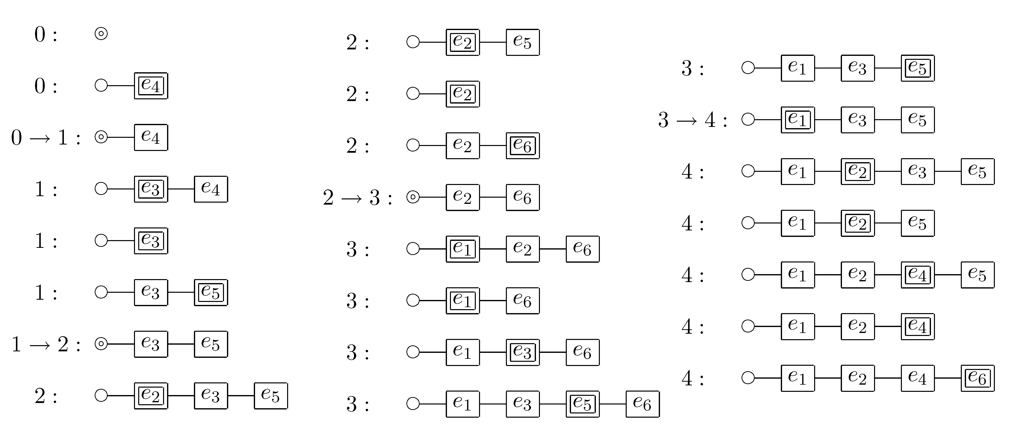To compute this part efficiently, we implement $E_{\text{HI}}$ as a doubly linked list (see Figure 5). For each step of the traversal, we memorize the position of the most recently inserted element into $E_{\text{HI}}$. Note that when we arrive at ⊤ and go back to the most recent branch node, we have to recover the corresponding position in some way e.g., by means of a stack. When we insert an element $e_i$ into $E_{\text{HI}}$, we put $e_i$ in the next position of the most recently inserted element. It can be easily verified that all elements placed before (respectively, after) the most recently inserted element are sorted in increasing order of their indices. Thus, in order to scan all elements $e_l\in E_{\text{HI}}$ with $i<l<j$, it suffices to search from the position of the most recently inserted element until the condition breaks. Since the total number of elements searched in a period is proportional to k, we obtain the time necessary to compute the function Update through a period.

Algorithm 2 Update the current partition p and the auxiliary data structures $G,B_{\text{new}},E_{\text{HI}}$ according to the current node f, the selected arc type of f, and the next node g

function Update(f, g, p, G, $B_{\text{new}}$, $E_{\text{HI}}$       $i\leftarrow \mathrm{V}\left(f\right)$; $j\leftarrow \mathrm{V}\left(g\right)$;       if the HI arc of f is selected and $e_i\notin E_{\text{HI}}$ then           $\text{Move}\left(e_i,p,G,B_{\text{new}}\right)$; $E_{\text{HI}}\leftarrow E_{\text{HI}}\cup \left\{e_i\right\}$;       else if the LO arc of f is selected and $e_i\in E_{\text{HI}}$ then           $\text{Move}\left(e_i,p,G,B_{\text{new}}\right)$; $E_{\text{HI}}\leftarrow E_{\text{HI}}\setminus \left\{e_i\right\}$;       end if       for all $e_l\in E_{\text{HI}}$ with $i<l<j$ do           $\text{Move}\left(e_l,p,G,B_{\text{new}}\right)$; $E_{\text{HI}}\leftarrow E_{\text{HI}}\setminus \left\{e_l\right\}$;       end for   end function function Move($e_i$, p, G, $B_{\text{new}}$)       $b\leftarrow$ the block of p which contains $e_i$;       if the child of b is not in $B_{\text{new}}$ then           Add a new empty block $b^{\prime }$ to p;           Add $b^{\prime }$ to G in such a way that $b^{\prime }$ has no child and the child of b is $b^{\prime }$;           $B_{\text{new}}\leftarrow B_{\text{new}}\cup \left\{b^{\prime }\right\}$;       end if       Move $e_i$ to the block corresponding to the child of b;       Delete b from p and G if b is empty;   end function

Let us consider the number of traversed nodes with repetition during the computation. Clearly the number of periods is $m+1$. For each $i(0\le i\le m)$, let $P_i$ denote the path traced in the i-th period, which starts with a branch node and ends with ⊤. The number of HI arcs in $P_i$ is bounded above by k. The head of each LO arc in $P_i$ is a branch node, since the LO arc of a non-branch node is not selected in our traversal. The LO arc of any branch node is traversed exactly once. Thus the total number of LO arcs traversed during the computation is m. Therefore, ${\sum }_{0\le i\le m}\left|P_i\right|\le (m+1)k+m$. We conclude that the time necessary to execute Algorithm 1 is proportional to $n+km$.

Figure 5. For each step of the traversal of the ZDD given in Figure 3, the doubly linked list of HI-state elements is shown below, where the index denotes the number of times ⊤ was visited and the double box or circle denotes the position after which an element is inserted.

Figure 5. For each step of the traversal of the ZDD given in Figure 3, the doubly linked list of HI-state elements is shown below, where the index denotes the number of times ⊤ was visited and the double box or circle denotes the position after which an element is inserted.

3.3. Conditional Co-occurrence Relations

Given a ZDD where every two elements are separable, Algorithm 1 cannot extract any useful information from the ZDD, but even so, we want to find some structural information hidden in the ground set. In this subsection we focus on the condition that enforces some elements always to be in a HI state and some elements always to be in a LO state.

Let (ON, OFF) be a pair of subsets of the ground set S of a ZDD. Two elements $e_i,e_j\in S$ are conditionally inseparable with respect to (ON, OFF) if they co-occur with each other for all paths that satisfy the condition: the HI arcs are always selected for all elements in ON; The LO arcs are always selected for all elements in OFF.

Before extracting this relation, we need a preprocessing so that we can trace only paths that satisfy the condition above. Recall that the cardinality of a node f is the number of paths from f to ⊤. It is known (see also Algorithm C and Exercise 208 in [12]) that given a ZDD, the cardinalities of all nodes in the ZDD can be computed in time proportional to the size of f. This computation can be done in a bottom-up fashion: The cardinalities of ⊥ and ⊤ are 0 and 1, respectively; the cardinality of each internal node is the sum of the cardinalities of the two children. Given a pair (ON, OFF), it is easy to change to be able to compute the numbers of paths from all internal nodes f to ⊤ that satisfy the condition concerning (ON, OFF). For convenience we call these numbers conditional cardinalities with respect to (ON, OFF).

To construct a conditional co-occurrence partition, change Algorithm 1 as follows.

• Return the initial partition if the conditional cardinality of the root is zero.
• The next node g of the current node f is the LO child if the conditional cardinalities of the two children are nonzero; else if the conditional cardinality of the LO child is zero, the HI child; else, the LO child.
• In the while block of Algorithm 1, the next node g is the LO child if the conditional cardinality of the HI child is zero; otherwise, the HI child.

Theorem 3.3 Let m be the number of branch nodes. Let n be the size of a ground set. The computation for a conditional co-occurrence partition can be done in time proportional to mn.

Proof. This theorem can be proved in a similar way to the proof in Theorem 3.2, but an upper bound for the number of the traversed nodes cannot be similarly calculated. Indeed, because of the change in the while block, we may have to select many LO arcs. At least we can say that the size of each path $P_i$ is at most n and the number of periods is at most $m+1$. Thus the time is proportional to $mn$.

Thanks to this theorem, when selecting a pair (ON, OFF), there is no need to worry about a rapid increase of computation time. This is in contrast to the case where we arbitrarily select paths and compute a co-occurrence partition from the selected paths. These paths are no longer compressed, and even if they can be compressed in some way, the size is generally irrelevant to the size of the original ZDD, and thus we cannot give a similar guarantee.

4. Examples

In this section we provide two examples. First, we applied our algorithm to two datasets commonly used in frequent itemset mining. The datasets we used are mushroom and pumsb obtained from the Frequent Itemset Mining Dataset Repository. The mushroom dataset contains characteristics of various species of mushrooms and the pumsb dataset contains census data for population and housing. In both datasets, each record consists of distinct item IDs, which indicate characteristics of the record. Each record is considered as a set of items and a dataset as a set family, thus both datasets can be represented as ZDDs (see Table 1). The parameters n and k given in Theorem 3.2 correspond to the number of distinct items that appear in a dataset and the maximum number of items in a record, respectively. Although the maximum item ID in the pumsb dataset is 7116 and the minimum item ID is 0, there are only 2113 distinct item IDs. Thus we normalized the ground set to be the set $\{1,2,\dots ,2113\}$ such that each element i in the set corresponds to the i-th item ID that appears in the pumsb dataset.

Table 1. The used datasets, where $n,k,m$ denote the parameters given in Theorem 3.2.

	#Records	#Items ($n$)	$k$	$m$	$n+km$	#ZDD Nodes
mushroom	8,124	119	23	288	6,743	791
pumsb	49,046	2,113	74	48,058	3,558,405	1,498,636

Table 1. The used datasets, where $n,k,m$ denote the parameters given in Theorem 3.2.

	#Records	#Items ($n$)	$k$	$m$	$n+km$	#ZDD Nodes
mushroom	8,124	119	23	288	6,743	791
pumsb	49,046	2,113	74	48,058	3,558,405	1,498,636

The computed partitions for the mushroom and the pumsb datasets are shown in Table 2, where the entries in the right table are shown as original pumsb item IDs. For example, in each record of the mushroom dataset, either elements 75 and 89 both appear or none of them do. Since items in the same block have the same behavior, when we want to find useful information from a ZDD, we need not distinguish between them. If the number of blocks is small, then various analyses on a ZDD can be efficiently performed on a small set of items by selecting one representative from each block. Thus our algorithm is useful. Unfortunately, without any constraints there are many blocks in both datasets; however, a few constraints may reduce the number of blocks significantly. For example, in the pumsb dataset, there are 2037 many blocks without any constraints, while the constraints $\text{ON}=\left\{5065\right\}$ and $\text{OFF}=\varnothing$ reduce the number to 71 (see Table 3 for other settings of constraints).

Table 2. The computed results for the mushroom dataset (left) and the pumsb dataset (right), where the blocks of single items are omitted in the left table and the blocks of at most two items are omitted in the right table. Each line corresponds to one block.

Table 2. The computed results for the mushroom dataset (left) and the pumsb dataset (right), where the blocks of single items are omitted in the left table and the blocks of at most two items are omitted in the right table. Each line corresponds to one block.

Table 3. The numbers of blocks in various settings of constraints ON and OFF in the pumsb dataset. In the left table, each line in the first column contains one item chosen at random for ON, where $\text{OFF}=\varnothing$; in the right table, each line in the first column contains five items chosen at random for OFF, where $\text{ON}=\varnothing$. Items are shown as original pumsb item IDs.

ON	#Blocks		OFF					#Blocks
5065	71		1	4744	4933	5894	6021	1,466
98	330		347	1469	4447	4503	4772	1,774
208	408		0	3280	4543	6052	6062	1,898
52	45		271	5695	6140	6405	7057	1,772
5375	12		2421	4656	5949	6159	6299	2,031

Table 3. The numbers of blocks in various settings of constraints ON and OFF in the pumsb dataset. In the left table, each line in the first column contains one item chosen at random for ON, where $\text{OFF}=\varnothing$; in the right table, each line in the first column contains five items chosen at random for OFF, where $\text{ON}=\varnothing$. Items are shown as original pumsb item IDs.

ON	#Blocks		OFF					#Blocks
5065	71		1	4744	4933	5894	6021	1,466
98	330		347	1469	4447	4503	4772	1,774
208	408		0	3280	4543	6052	6062	1,898
52	45		271	5695	6140	6405	7057	1,772
5375	12		2421	4656	5949	6159	6299	2,031

As a second example, we applied the algorithm for the conditional case to a set of paths enumerated from the graph given in Figure 6. We considered paths from the vertex 01 to the vertex 47 of the graph such that no vertices are visited twice, which are called simple paths. Since simple paths can be identified with sets of edges, the set of all simple paths from 01 to 47 can be represented as a ZDD whose ground set corresponds to the edge set of the graph. The number of such simple paths turns out to be 14,144,961,271, while the corresponding ZDD in our ordering of the edge set has only 599 branch nodes (see Table 4). This is in contrast to the pumsb dataset in the previous example, where the number of branch nodes is roughly the same as the number of records represented by a ZDD. The ZDD of the present example can be quickly constructed in a top-down fashion. This technique has been described in the literature; see, e.g., [5,12], (Exercise 225 in §7.1.4). We analyzed which edges co-occur with each other for all simple paths with the constraints ON and OFF given in Figure 6. The computed partition is shown in the right table of Figure 6. As we showed in Theorem 3.3, once we obtain a small ZDD like in this case, we can quickly compute co-occurrence partitions in various settings of ON and OFF.

Figure 6. We considered simple paths from the vertex 01 to the vertex 47. When the edge set ON consists of bold edges and OFF consists of dashed edges, the blocks of the corresponding co-occurrence partition except for blocks of single edges are shown in the right table as the collections of edges separated by horizontal lines.

Figure 6. We considered simple paths from the vertex 01 to the vertex 47. When the edge set ON consists of bold edges and OFF consists of dashed edges, the blocks of the corresponding co-occurrence partition except for blocks of single edges are shown in the right table as the collections of edges separated by horizontal lines.

Table 4. The ZDD representing simple paths from the vertex 01 to the vertex 47, where $n,k,m$ denote the parameters given in Theorem 3.2.

Start	End	#Paths	#Edges ($n$)	$k$	$m$	$n+km$	#ZDD Nodes
01	47	14,144,961,271	92	44	599	26,448	1,085

Table 4. The ZDD representing simple paths from the vertex 01 to the vertex 47, where $n,k,m$ denote the parameters given in Theorem 3.2.

Start	End	#Paths	#Edges ($n$)	$k$	$m$	$n+km$	#ZDD Nodes
01	47	14,144,961,271	92	44	599	26,448	1,085

In order to enumerate simple paths and construct ZDDs, we used the Stanford GraphBase, the simpath and the simpath-reduce programs by Knuth [13,14]. Furthermore, in both examples we used the Colorado University Decision Diagram Package by Somenzi [15].

5. Conclusions

We presented the following basic algorithm of ZDDs: Given a ground set S and a ZDD that represents a collection of subsets of S, the algorithm extracts a hidden structure, called a co-occurrence relation, on S from the ZDD. We furthermore introduced conditional co-occurrence relations and presented an extraction algorithm, which enables us to discover further structural information. We showed that these computations can be done in time complexity that is related not to the number of sets, but to some feature values of a ZDD. Our algorithms are effective especially when a large number of sets are compressed into a small ZDD.

References

1. Minato, S. Zero-Suppressed BDDs for Set Manipulation in Combinatorial Problems. In Proceedings of 30th ACM/IEEE Design Autiomation Conference (DAC-93), Dallas, TX, USA, June 1993; pp. 272–277.
2. Minato, S.; Arimura, H. Efficient Method of Combinatorial Item Set Analysis Based on Zero-Suppressed BDDs. In Proceedings of IEEE/IEICE/IPSJ International Workshop on Challenges in Web Information Retrieval and Integration (WIRI-2005), Tokyo, Japan, April 2005; pp. 3–10.
3. Minato, S.; Arimura, H. Frequent closed item set mining based on zero-suppressed BDDs. Trans. Jpn. Soc. Artif. Intell. 2007, 22, 165–172. [Google Scholar] [CrossRef]
4. Coudert, O. Solving Graph Optimization Problems with ZBDDs. In Proceedings of the 1997 European Conference on Design and Test, Paris, France, March 1997; pp. 224–228.
5. Sekine, K.; Imai, H. A Unified Approach via BDD to the Network Reliability and Path Numbers. In Technical Report 95-09; Department of Information Science, University of Tokyo, 1995. [Google Scholar]
6. Akers, S.B. Binary decision diagrams. IEEE Trans. Comput. 1978, 27, 509–516. [Google Scholar] [CrossRef]
7. Bryant, R.E. Graph-Based algorithms for boolean function manipulation. IEEE Trans. Comput. 1986, 35, 677–691. [Google Scholar] [CrossRef]
8. Lampka, K.; Siegle, M.; Ossowski, J.; Baier, C. Partially-Shared zero-suppressed multi-terminal BDDs: Concept, algorithms and applications. Form. Methods Syst. Des. 2010, 36, 198–222. [Google Scholar] [CrossRef]
9. Minato, S. Finding Simple Disjoint Decompositions in Frequent Itemset Data Using Zero-Suppressed BDDs. In Proceedings of IEEE ICDM Workshop on Computational Intelligence in Data Mining, Houston, TX, USA, November 2005; pp. 3–11.
10. Minato, S.; Ito, K. Symmetric item set mining method using zero-suppressed bdds and application to biological data. Trans. Jpn. Soc. Artif. Intell. 2007, 22, 156–164. [Google Scholar] [CrossRef]
11. Minato, S. A Fast Algorithm for Cofactor Implication Checking and Its Application for Knowledge Discovery. In Proceedings of IEEE 8th International Conference on Computer and Information Technology (CIT 2008), Sydney, Australia, July 2008; pp. 53–58.
12. Knuth, D.E. The Art of Computer Programming Volume 4a; Addison-Wesley Professional: New Jersey, NJ, USA, 2011. [Google Scholar]
13. Knuth, D.E. The Stanford GraphBase. Available online: http://www-cs-faculty.stanford.edu/uno/sgb.html (accessed on 4 September 2012).
14. Knuth, D.E. SIMPATH and SIMPATH-REDUCE. Available online: http://www-cs-faculty.stanford.edu/uno/programs.html (accessed on 4 September 2012).
15. Somenzi, F. CUDD: CU Decision Diagram Package: Release 2.5.0. Available online: http://vlsi.colorado.edu/fabio/CUDD/ (accessed on 4 September 2012).