A Sensor-Based Learning Algorithm for the Self-Organization of Robot Behavior

Abstract

Ideally, sensory information forms the only source of information to a robot. We consider an algorithm for the self-organization of a controller. At short time scales the controller is merely reactive but the parameter dynamics and the acquisition of knowledge by an internal model lead to seemingly purposeful behavior on longer time scales. As a paradigmatic example, we study the simulation of an underactuated snake-like robot. By interacting with the real physical system formed by the robotic hardware and the environment, the controller achieves a sensitive and body-specific actuation of the robot.

1. Introduction

Despite the tremendous progress in hardware and in both sensorial and computational efficiency, the performance of contemporary autonomous robots does not reach that of simple animals. This situation has triggered an intense search for alternative approaches to the control of robots. The present paper exemplifies homeokinesis [1, 2], a general approach to the self-organization of behavior which is based on the dynamical systems approach to robot control cf. e.g. [3,4,5] and may be understood as a dynamical counterpart of the principle of homeostasis.

According to the homeostatic principle [6, 7], behavior results from the compensation of perturbations of an internal homeostatic equilibrium. Although this approach proves successful in simple systems [8, 9], it remains elusive how it scales up to situations, where, e.g., internal nutrient levels in an agent are to give rise to the specific form of a resulting complex behavior.

Homeokinesis, in contrast, provides a mechanism for the self-organization of elementary movements that are not directly caused by a triggering stimulus, but are generated by amplification of intrinsic or extrinsic noise which is counterbalanced by the simultaneous maximization of the predictability of the resulting behavior. Homeokinesis provides a mechanism to produce behaviors that are not brought about by a reward signal or a prescribed target state, but that minimize an internal error functional based on sensory information [10].

We will investigate a robotic device with a complex physical behavior that is controlled according to the homeokinetic principle. Starting with an inactive robot and an unspecifically initialized controller, movements are generated in the beginning by amplifying noisy sensory inputs. At the same time the parameters of the controller are adapted according to the changes in the sensor values that are observed following the execution of actions. In the course of the adaptation, the generated actions increasingly match the properties of the robotic device in its environment as observed by the sensors. In the case of the snake-like robot this leads to a rotational mode of behavior of the whole body resulting from the self-organization of the control. The principles of the self-organized control will be briefly sketched in the next section. Section 3. presents the application to an underactuated physical system of many degrees of freedom. Conclusions are stated in Section 4.

2. Self-organizing Dynamical Systems

Altering Aristotle we may state that there is nothing in behavior that was not first in the senses. Let us therefore consider a robot that receives at each instant of time, $t=0,1,\dots$, a vector of sensor values $x_t\in {\mathbb{R}}^n$. The controller is determined by a function K mapping sensor values $x\in {\mathbb{R}}^n$ to motor values $y\in {\mathbb{R}}^m$

$$y=K\left(x\right),$$

where all variables refer to time step t. The controller is adaptive and depends on a set of adjustable parameters. In the cases considered below, these are the parameter matrix $c\in {\mathbb{R}}^{m\times n}$ and a parameter vector $h\in {\mathbb{R}}^m$. The controller is thus given by a pseudolinear expression

$$K_i\left(x\right)=g\left(z_i\right),i=1,\cdots ,m,$$

(1)

where

$$z_i=\sum _j{c}_{ij}{x}_j+h_i$$

(2)

and g is an componentwise nonlinearity that assures the boundedness of the motor output $y_i$. We choose here $g\left(z\right)=tanh\left(z\right)$. The controller can be interpreted as a system of m artificial neurons. For each neuron the membrane potential $z_i$ is calculated by the weighted sum of the inputs $x_j$, $j=1,\cdots ,n$ and the threshold $h_i$, while the motor output is determined by applying the nonlinearity to $z_i$.

The robot behavior is generated by the interplay of the state dynamics and the fast parameter adaptation (see Equation 11 below) such that the simple control scheme produces highly nontrivial results.

2.1. World Model and Sensorimotor Dynamics

We assume that the robot has the ability of gaining knowledge about the robotic body and the environment which is realized by an internal model $F:{\mathbb{R}}^n\times {\mathbb{R}}^m\to {\mathbb{R}}^n$. The model learns to associate the actions y of the robot with new sensor values in order to predict future inputs

$$x_{t+1}=F\left(x_t,y_t\right)+{\xi }_t.$$

(3)

The model error ${\xi }_t$ is used to train the model F by supervised learning.

In the example considered below we assume that the response of the sensor is linearly related to the motor command, i.e. we can write

$$x_{t+1}=a{y}_t+{\xi }_t,$$

(4)

where a is a matrix and the error ξ is considered to be random. The parameters of the model are adapted by gradient descent

$$\Delta a={\epsilon }_M\xi y^T,$$

(5)

where both ξ and y are taken at time t and ${\epsilon }_M$ is the learning rate. The simplicity of the model is compensated by the fact that the learning rate will be high so that the model changes rapidly in order to match different world situations by relearning. Moreover, there is no need that the model represents the full complexity of the environment, because the behavior is adapted based on the model. The behaviors that can be generated by the homeokinetic controller are thus restricted by the complexity of the model. Because the model is adaptive and adaptation can be fast for a linear model, the simplicity of the model affects only the local properties of the trajectory. A linear model is thus a way to introduce smooth trajectories. If the robot encounters strong nonlinearities in the environment, e.g. when bumping into a wall, then a large error is produced that has a drastic effect on the parameters of both the controller and the internal model.

With the above notions we can write the dynamics of the sensorimotor loop in a closed form

$$x_{t+1}=\psi \left(x_t\right)+{\xi }_t,$$

(6)

where the dynamics of the system is expressed by the loop function

$$\psi \left(x\right)=aK\left(x\right),$$

which depends on the parameters of both the model and the controller.

2.2. Realizing Self-Organization

As known from physics, self-organization typically results from the compromise between a driving force that amplifies fluctuations and a regulating force that tends to stabilize the system. Here destabilization is achieved by increasing the sensitivity of the sensory response, which is induced by control based on previous sensor values. The counteracting force is obtained from the requirement that the consequences of the actions taken are still predictable. Details may be found in Reference [10]. We formulate these complementary goals into an objective function

$$E_t={\xi }_t^T{Q}_t^{-1}{\xi }_t$$

(7)

where ξ is the model error introduced above, $Q=L{L}^T$ is a positive semidefinite matrix, and L is the Jacobi matrix of the sensorimotor dynamics, i.e. $L_{ij}\left(x\right)=\frac{\partial }{\partial x_j}{\psi }_i\left(x\right)$. In the present case we have

$$L_{ij}\left(x\right)=\sum _{k=1}^n{a}_{ik}{g}^{\prime }\left(z_k\right)c_{kj},$$

(8)

where $g^{\prime }\left(z_k\right)=\frac{\partial }{\partial x_j}g\left(z_k\right)$ and all quantities refer to time t. Using gradient descent with a learning rate ε, the parameters of the controller follow the dynamics

$$\Delta c_t=-\epsilon \frac{\partial E_t}{\partial c_t}\left(x_t,c_t\right).$$

(9)

Explicit expressions for the parameter dynamics are given below (11). Note that the parameter dynamics Equation 9 is updated at each time step so that the parameters change practically on the behavioral time scale. This means that the parameter dynamics is constitutive for the behavior of the robot.

The expression Equation 7 represents the essence of our approach. The matrix Q measures the sensitivity of the sensorimotor loop towards changes in the sensor values. Minimizing E is thus immediately seen to increase this sensitivity since E contains the inverse of Q. We have shown in many practical applications that robots generate explorative behavior as a consequence of the minimization of E (7). The exploration is, however, not random, but moderated by the fact that E is also small if the prediction error ξ is small which is the case for smooth behaviors. Behavior can thus be understood as a compromise between the two opposing goals sensibility and predictability.

2.3. Explicit Parameter Dynamics

We will now derive the explicit parameter dynamics for a robot with two sensors and two actuators that will be used in the next Section. In order adapt the controller according to Equation 9, we must invert the matrix Q. This is easy in the two dimensional case such that explicit expressions for the parameter dynamics can be obtained. We observe that the parameters occur also in the derivative of the output functions $g^{\prime }$ which can be treated as

$$\frac{\partial }{\partial c_{ik}}{g}_j^{\prime }={\delta }_{ij}{g}_i^{″}\frac{\partial z_i}{\partial c_{ik}}={\delta }_{ij}{g}_i^{″}{x}_k,$$

where ${\delta }_{ij}$ is the Kronecker delta. In the case $g\left(z\right)=tanh\left(z\right)$, we have $g^{″}\left(z\right)=-2g{g}^{\prime }$ such that

$$\frac{\partial }{\partial c_{ik}}{g}_j^{\prime }=-2{\delta }_{ij}{g}_i^{\prime }{y}_i{x}_k$$

(10)

The explicit formulas are

$$\begin{array}{cc}\hfill {\epsilon }^{-1}\Delta c_{ij}& ={\zeta }_i{v}_j-2{\zeta }_i{\rho }_i{y}_i{x}_j\hfill \\ \hfill {\epsilon }^{-1}\Delta h_i& =-2{\zeta }_i{\rho }_i{y}_i\hfill \end{array}$$

(11)

where ${\zeta }_i=g_i^{\prime }{\mu }_i$, $\mu =a^T{Q}^{-1}\xi$, $\rho =cv$, and $v=L^{-1}\xi$. All quantities refer to the same time step t and a suitable regularization has to be used if L is singular.

We may interpret the first term ${\zeta }_i{v}_j$ as a general driving term which is seen to increase the sensitivity of the linearized sensorimotor loop. The second term contains the effects of the nonlinearity (10) and essentially keeps the output away from saturation which implies sensitivity to the inputs. This term may be interpreted as an (anti-)Hebbian learning contribution with strength $2{\zeta }_i{\rho }_i$. The dynamics of the threshold h is driven exclusively by this term.

The learning parameter ε is chosen such that the parameters change at about the same time scale as the behavior, i.e. parameter configurations corresponding to generated behaviors are not preserved by the control system. Hence, the system can be said to show rather adaptation than learning. This flexibility should not be considered as a drawback of the approach. It is straightforward to store controller configurations in a long-term memory if the behavior persists for some time or receives any external reward. The stored behaviors can be re-used at later encounters with similar sensory inputs or can be accessed for planning or for further optimization of a particular behavior.

3. Experiments

The robot that we have chosen for the experiments is called “skidding snake”. It consists of ten massive spheres, each with a diameter of $0.17$ length units. The spheres are connected to each other by a ball-and-socket joint, see Figure 2(a) such that each of the spheres can rotate passively like in a string of beads. Only one sphere, the head element, is driven by forces parallel to the ground which may be understood as a force vector $y_t\in {\mathbb{R}}^2$ of arbitrary direction (see Figure 2(b)). The sensor values are the velocities of the head relative to the ground, i.e. we measure a vector $x_t={\left(x_1^t,x_2^t\right)}^T$ where time is written as an upper index when indicating the components of a vector. Sensor and motor values are normalized to the range $[-1,1]$. One time step is $0.01$ seconds. The robot is placed in a rectangular arena of 10x10 length units surrounded by walls. In a physical realization the head may be a robot with omnidirectional drive, see e.g. [11].

The robot is underactuated in the sense that the force acting on the head is not sufficient to drag the tail into arbitrary directions due to a considerable friction of the spheres on the ground. Instead only more or less lateral motions of the head are possible. Nevertheless, as we will see in the simulations, the controller can excite whole-body motions by exploiting inertia and gyroscopic effects. These physical effects are found by the self-organizing controller as a means for accumulating sufficient energy in order to move the full body in spite of underactuation.

The experiment starts with model and controller parameters (matrices a and c) initialized as unit matrices and the adaptive thresholds h set to zero. In the initial phase of the experiment, random forces applied to the head element lead to small lateral motions of the head swaying the tail occasionally passively around. The sensor values x and controller outputs y are fluctuating around zero, as a consequence of these movements, see Figure 2. Therefore, the parameter changes $\Delta c_{ij}$ in Equation 11 are dominated by the driving term ${\zeta }_i{v}_j$ and the off-diagonal matrix elements of c increase (see Fig 3 top) so that the reaction of the head to its sensor values becomes more and more sensitive. The amplitude of the controller output increases due to the amplification of the noise. There is still no coherent reaction of the body to these random signals which is seen from the fact that the sensor values keep fluctuating around zero during the first 18000 steps.

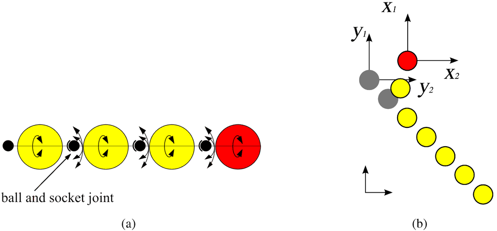
Figure 1. (a) Mechanical construction of the skidding snake. Ball-and-socket joints between the spheres are drawn. Arrows indicate the possible rotations: in every direction at the joint and around the axis between joints. (b) Sketch of the robot in the global coordinate system. After execution of a time step in which the motor vector y was applied to the head element the sensor vector x is read back as feedback of the system. The components of the motor vector y and the sensor vector x are aligned with the axes of the global coordinate system.

Figure 1. (a) Mechanical construction of the skidding snake. Ball-and-socket joints between the spheres are drawn. Arrows indicate the possible rotations: in every direction at the joint and around the axis between joints. (b) Sketch of the robot in the global coordinate system. After execution of a time step in which the motor vector y was applied to the head element the sensor vector x is read back as feedback of the system. The components of the motor vector y and the sensor vector x are aligned with the axes of the global coordinate system.

With increasing sensitivity, the controller also starts to respond to the swaying of the body and manages to amplify the latter. This process is self-organizing since the emerging rotational whole-body motions respond to the controller in a much more predictable way. Thus, in the long run the controller supports these motions of all elements. The body is seen at first meandering and eventually becoming engaged in a rotational mode where the body becomes stiff like a stick due to the gyroscopic effects of the rapidly rotating spheres of the body, see Figure 4. The diagram in Figure 5 shows the sensory and motor space, where transitions to temporary stable limit cycles represent the rotational mode of the skidding snake. Videos of the behavior are available at [12].

In the present experiment the emergence of coordinated behavior occurs from step 18000 corresponding to about three minutes simulated real time. By then the sensor values increase largely and indicate that the controller has achieved the capability of exciting the system. Due to the rapid increase of the sensor values the controller neurons are transferred to near the saturation region, see Figure 2 bottom. This leads to an increase of the anti-Hebbian term in the parameter dynamics Equation 11. In this way the controller parameters are decreased again and the system leaves the saturation region as part of the large-scale behavioral cycle. The power spectrum of the sensor value $x_1$ indicates the rotational mode of behavior by the appearance of the red line corresponding to the frequency of rotation, see Figure 6. The energy of the frequency components before the rotational mode is much lower and hence barely visible even for the logarithmic color scale of the diagram. The decrease of the frequency of rotation around step 29000 is caused by a collision with the walls of the arena in which the snake is located. After the collision the frequency increases again to its pre-collision value.

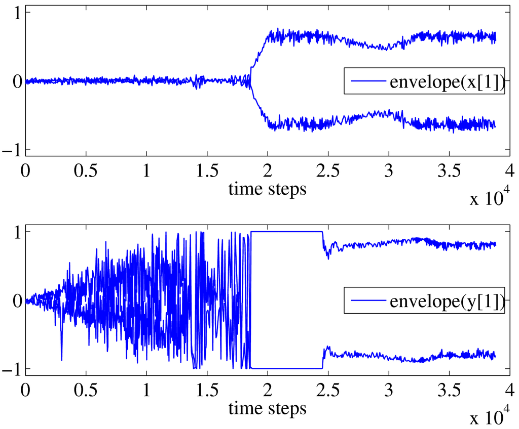
Figure 2. Envelopes of sensor value $x_1$ and motor value $y_1$ during the experiment. The envelopes of the signals are shown, since due to the fast oscillations also in a signal plot only the envelopes can be identified. Top: Sensor value $x_1$ fluctuates around zero at the beginning, because the applied forces lead only to small lateral motions of the head with the tail sometimes swaying around passively. With increasing sensitivity the controller starts to respond to the swaying of the body leading to a rotational mode of behavior (second half of the diagram). Bottom: Controller output $y_1$ also fluctuates around zero in the beginning, but with increasing sensitivity of the controller the amplitude increases, the controller responds to the swaying of the body eventually leading to a rotational mode. Plots for $x_2$ and $y_2$ look similar.

Figure 2. Envelopes of sensor value $x_1$ and motor value $y_1$ during the experiment. The envelopes of the signals are shown, since due to the fast oscillations also in a signal plot only the envelopes can be identified. Top: Sensor value $x_1$ fluctuates around zero at the beginning, because the applied forces lead only to small lateral motions of the head with the tail sometimes swaying around passively. With increasing sensitivity the controller starts to respond to the swaying of the body leading to a rotational mode of behavior (second half of the diagram). Bottom: Controller output $y_1$ also fluctuates around zero in the beginning, but with increasing sensitivity of the controller the amplitude increases, the controller responds to the swaying of the body eventually leading to a rotational mode. Plots for $x_2$ and $y_2$ look similar.

There is an interesting interplay between the parameter dynamics of the world model and the controller. In the beginning the model parameters are decreasing (first 3000 steps), see Figure 3 center, since the reaction of the head to the applied forces is weak because the controller is not yet able to excite the whole-body modes of the robotic device. Around step 18000 the controller starts to become effective so that there is a definite response of the body to the controller actions which is reflected by an increase of the diagonal elements of the matrix a.

Later on the controller reduces its reaction strength to the inputs. This can be expected since the forces necessary to keep the system in the rotational mode are much smaller. The combined action of c and a is reflected in the response matrix R of the linearized sensorimotor loop. Figure 3 shows a steep rise in the response of the system when the rotational mode is emerging. After a stable period the response matrix is seen to decrease and at the end of the rotational period it is seen to have a pronounced SO(2) form (i.e. R is close to a rotation matrix, see e.g. [13]) reflecting the fact that the system is in a well controlled rotational mode of lower frequency. This rotational mode is reflected in the transition to temporary stable limit cycles in the sensor and motor space in Figure 5. Quite generally, the response strength self-regulates to a slightly supercritical value unless the system encounters unexpected responses from the environment.

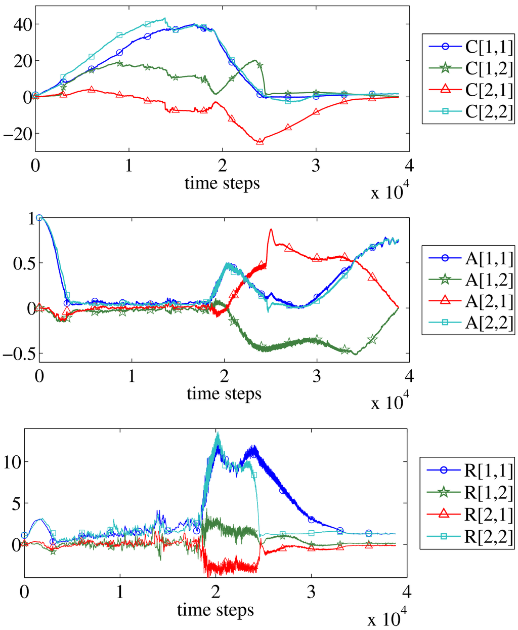
Figure 3. Parameters during the experiment. Top: Matrix c of controller parameters showing the increase of sensitivity, in the first half of the diagram, while in the second half when the rotational whole-body motion sets in the reaction strength is turned down since there is a definite response of the body to the controller actions even with smaller parameter values. Center: Matrix a of model parameters shows the correlation between sensor and motor values. At the beginning there is a decrease from the initial values to the ones representing the weak reaction of the head element to the controller outputs. After step 18000 when the rotational mode sets in the diagonal elements increase since there is a definite response of the body to the controller actions. Bottom: The response matrix R of the system shows a steep rise when the rotational mode emerges. After a stable period the response strength decreases, showing a SO(2)-like form at the end of the experiment reflecting the systems rotational mode of lower frequency. It is seen that the response strength is self-regulating to a slightly supercritical value if the system gives valuable response.

Figure 3. Parameters during the experiment. Top: Matrix c of controller parameters showing the increase of sensitivity, in the first half of the diagram, while in the second half when the rotational whole-body motion sets in the reaction strength is turned down since there is a definite response of the body to the controller actions even with smaller parameter values. Center: Matrix a of model parameters shows the correlation between sensor and motor values. At the beginning there is a decrease from the initial values to the ones representing the weak reaction of the head element to the controller outputs. After step 18000 when the rotational mode sets in the diagonal elements increase since there is a definite response of the body to the controller actions. Bottom: The response matrix R of the system shows a steep rise when the rotational mode emerges. After a stable period the response strength decreases, showing a SO(2)-like form at the end of the experiment reflecting the systems rotational mode of lower frequency. It is seen that the response strength is self-regulating to a slightly supercritical value if the system gives valuable response.

Figure 4. The rotational mode of behavior is characterized by a rotation of all spheres around their axis (connection between the joints), where the first half of the spheres rotate in the opposite direction than the other half. Hence the whole snake rotates around its center and in doing so becomes stiff like a stick.

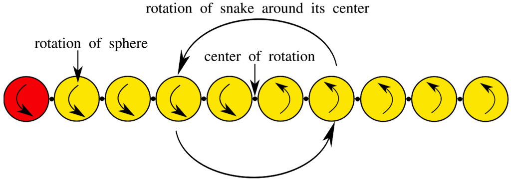
Figure 4. The rotational mode of behavior is characterized by a rotation of all spheres around their axis (connection between the joints), where the first half of the spheres rotate in the opposite direction than the other half. Hence the whole snake rotates around its center and in doing so becomes stiff like a stick.

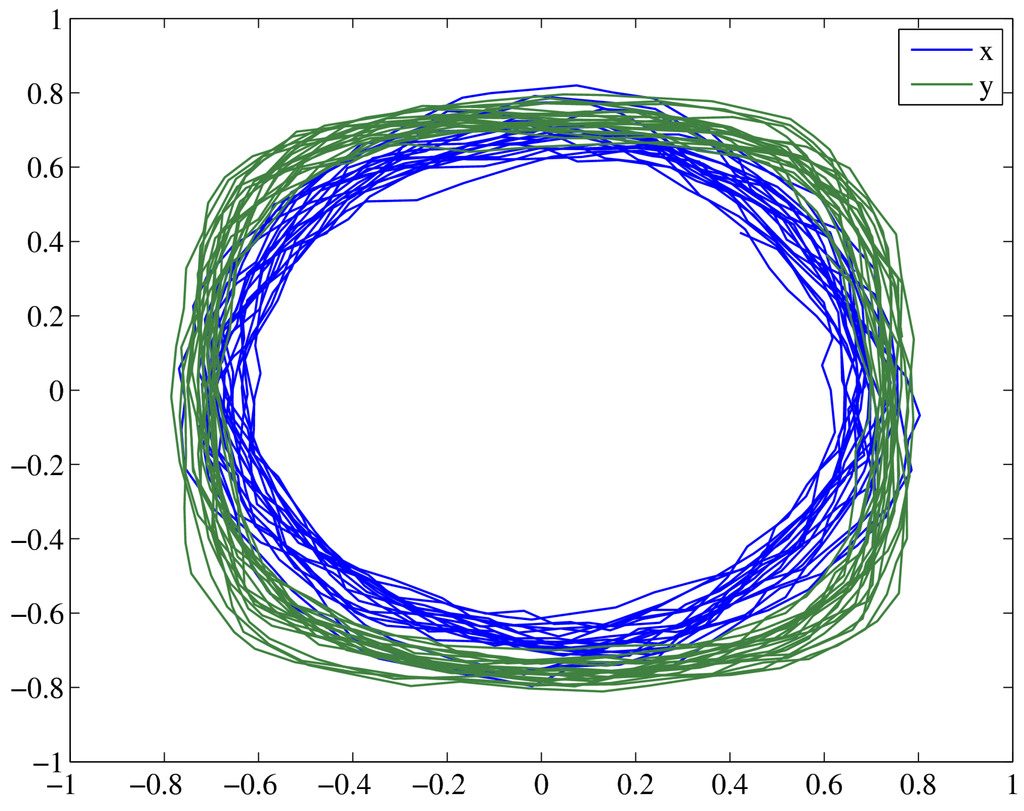
Figure 5. Motor space (blue line) and sensor space (green line) show the temporary stable rotational mode of the skidding snake (1000 time steps plotted).

Figure 5. Motor space (blue line) and sensor space (green line) show the temporary stable rotational mode of the skidding snake (1000 time steps plotted).

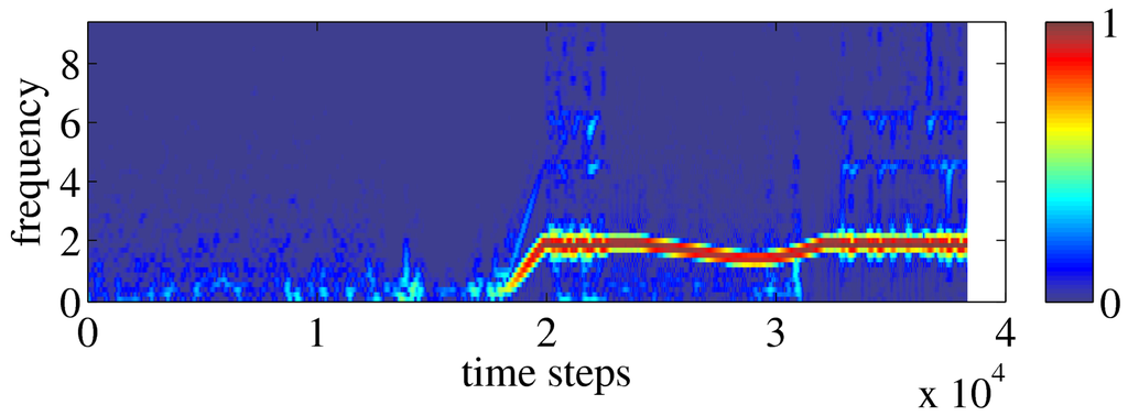
Figure 6. Power spectrum of the sensor value $x_1$ (measured velocity) with a logarithmic color scale during the experiment. Each column represents the lower frequency part of the discrete Fourier transform of a five second sliding window of the sensor value. Every time step a power spectrum is plotted. Blue pixels of the logarithmic color scale correspond to low energy and red to high energy in the corresponding frequency band. High energy in a certain frequency band means that changes between positive and negative velocity in the sensor value occur at about that frequency. The energy is normalized by the maximal energy in the power spectrum. In the beginning of the experiment no favorite frequency of behavior can be identified in the system. The start of the rotational mode of behavior is indicated by the appearance of the red line showing the frequency of rotation (around step 18000). During the rotational mode this frequency decreases due to a collision with a wall of the arena. After the collision the frequency increases again to the pre-collision value. The energy of the frequency of rotation is much larger as compared to the frequency components before this motion sets in. Hence the diagram shows only light blue dots before the rotational mode. The power spectrum of the sensor value $x_2$ looks similar.

Figure 6. Power spectrum of the sensor value $x_1$ (measured velocity) with a logarithmic color scale during the experiment. Each column represents the lower frequency part of the discrete Fourier transform of a five second sliding window of the sensor value. Every time step a power spectrum is plotted. Blue pixels of the logarithmic color scale correspond to low energy and red to high energy in the corresponding frequency band. High energy in a certain frequency band means that changes between positive and negative velocity in the sensor value occur at about that frequency. The energy is normalized by the maximal energy in the power spectrum. In the beginning of the experiment no favorite frequency of behavior can be identified in the system. The start of the rotational mode of behavior is indicated by the appearance of the red line showing the frequency of rotation (around step 18000). During the rotational mode this frequency decreases due to a collision with a wall of the arena. After the collision the frequency increases again to the pre-collision value. The energy of the frequency of rotation is much larger as compared to the frequency components before this motion sets in. Hence the diagram shows only light blue dots before the rotational mode. The power spectrum of the sensor value $x_2$ looks similar.

4. Discussion

The homeokinetic paradigm is formulated mathematically based on the error function (7, 8) which implies the parameter dynamics Equation 11. We have demonstrated that this general scheme is applicable to the control of an unknown body with complex physical properties. Homeokinetic control leads to an active behavior that extracts physical properties of the system from the sensory information and selects behavioral modes where the control is most effective. This corresponds here to the excitation of whole-body motions which cannot be affected by single control actions in an underactuated system. These modes are not persistent but metastable so that the system more or less tries to investigate its behavioral possibilities. Moreover this scenario is stable under strong influences by the environment both of a static and a dynamic nature (other agents), see the videos [12].

An important observation can be derived for the interplay between the world model and the controller. The system does not have information on the structure and dynamics of the body so that the world model learns this relation from scratch by observing the sensory response to the actions taken. The so-called learning paradox has been discussed by several authors [14,15,16]. It refers to the problem that in order to control a robot, information of the reactions of the body is required while this information can only be acquired by sensible control. The homeokinetic paradigm can be seen as a solution of this problem which is sometimes also referred to as the cognitive bootstrapping problem. The concerted manner by which both the controller and the world model evolve during the emergence of the rotational mode seems to be a good example of this process.

Figure 7. Images of skidding snakes. Far left: Initial position in an experiment with three skidding snakes. Left: Close view of three skidding snakes in the beginning of an experiment. Right: Later on in the experiment: Two snakes are in the rotational mode where the bodies become stiff like sticks due to the gyroscopic effects of the rapidly rotating spheres of the body. The third is in z-shape with the tail passively swaying around. Far right: A group of interacting self-organized creatures under homeokinetic control. The three white balls are not actuated. The systems try different modes of behavior (including the rotational mode of the skidding snake) even under perturbations by other active agents. See also the videos [12].

Figure 7. Images of skidding snakes. Far left: Initial position in an experiment with three skidding snakes. Left: Close view of three skidding snakes in the beginning of an experiment. Right: Later on in the experiment: Two snakes are in the rotational mode where the bodies become stiff like sticks due to the gyroscopic effects of the rapidly rotating spheres of the body. The third is in z-shape with the tail passively swaying around. Far right: A group of interacting self-organized creatures under homeokinetic control. The three white balls are not actuated. The systems try different modes of behavior (including the rotational mode of the skidding snake) even under perturbations by other active agents. See also the videos [12].

We consider the homeokinetic approach as a novel contribution to the self-organization of complex robotic systems. At the present stage of development, the behaviors although related to the specific bodies and environments are without goal. However, when watching such behaving systems, one often observes behavioral sequences which might be helpful in reaching a specific goal. In future work we will focus on methods to shape the generated behaviors, see e.g. [17], in order to allow the robot to generate more complex behaviors and solve tasks by building on primitive behaviors according to the goals of developmental and epigenetic robotics [18, 19].

References and Notes

- Der, R.; Steinmetz, U.; Pasemann, F. Homeokinesis - A new principle to back up evolution with learning. In Computational Intelligence for Modelling, Control, and Automation; IOS Press: Amsterdam, Demark, 1999; Concurrent Systems Engineering Series; Vol. 55, pp. 43–47. [Google Scholar]
- Der, R.; Herrmann, M.; Liebscher, R. Homeokinetic approach to autonomous learning in mobile robots. In Robotik 2002; Dillman, R., Schraft, R. D., Wörn, H., Eds.; VDI: Dusseldorf, Germany, 2002; pp. 301–306. [Google Scholar]
- Schöner, G.; Dose, M. A dynamical systems approach to task-level system integration used to plan and control autonomous vehicle motion. Robot. Auton. Systems 1992, 10, 253–267. [Google Scholar] [CrossRef]
- Steels, L. A case study in the behavior-oriented design of autonomous agents. In Proc. Third International Conference on Simulation of Adaptive Behavior: From Animals to Animats (SAB94), 1994; MIT Press: Cambridge, MA, USA, 1994; pp. 445–452. [Google Scholar]
- Tani, J.; Ito, M. Self-organization of behavioral primitives as multiple attractor dynamics: A robot experiment. IEEE Trans. Syst. Man Cybern. Part A: Systems and Humans 2003, 33, 481–488. [Google Scholar] [CrossRef]
- Cannon, W. B. The Wisdom of the Body; Norton: New York, USA, 1939. [Google Scholar]
- Ashby, W. R. Design for a Brain; Chapman and Hill: London, UK, 1954. [Google Scholar]
- Di Paolo, E. Organismically-inspired robotics: Homeostatic adaptation and natural teleology beyond the closed sensorimotor loop. In Dynamical Systems Approach to Embodiment and Sociality; Murase, K., Asakura, T., Eds.; 2003; pp. 19–42. [Google Scholar]
- Williams, H. Homeostatic plasticity in recurrent neural networks. In From Animals to Animats, Proc. 8th International Conference on Simulation of Adaptive Behavior; Schaal, S., Ispeert, A., Eds.; MIT Press: Cambridge, MA, USA, 2004; Vol. 8, pp. 344–353. [Google Scholar]
- Der, R.; Hesse, F.; Martius, G. Rocking stamper and jumping snake from a dynamical system approach to artificial life. Adapt. Behav. 2006, 14, 105–115. [Google Scholar] [CrossRef]
- Rojas, R.; Förster, A. Holonomic control of a robot with an omnidirectional drive. KI - Künstliche Intelligenz 2006, 20, 12–17. [Google Scholar]
- Der, R.; Hesse, F.; Martius, G. Videos of self-organized robot behavior. http://robot.informatik.uni-leipzig.de/Videos 2008.
- Pasemann, F.; Hild, M.; Zahedi, K. SO(2)-networks as neural oscillators. In Computational Methods in Neural Modeling; Mira, J., Alvarez, J., Eds.; Springer-Verlag: Heidelberg, Germany, 2003; pp. 144–151. [Google Scholar]
- Bereiter, C. Towards a solution to the learning paradox. Rev. Edu. Res. 1985, 55, 201–226. [Google Scholar] [CrossRef]
- Steffe, L. The learning paradox: A plausible counterexample. In Epistomological foundations of mathematical experience; Steffe, L., Ed.; Springer: New York, USA, 1991; pp. 26–44. [Google Scholar]
- von Glasersfeld, E. Scheme theory as a key to the learning paradox. In 15th Advanced Course; Archives Jean Piaget: Geneva, Switzerland, 1998. [Google Scholar]
- Hesse, F.; Der, R.; Herrmann, J. M. Reflexes from self-organizing control in autonomous robots. In Proc. 7th International Conference on Epigenetic Robotics: Modelling Cognitive Development in Robotic Systems, Rutgers University, Piscataway, NJ, USA; Berthouze, L., Prince, C., Littman, M., Kozima, H., Balkenius, Ch., Eds.; Lund University Press: Lund, Sweden, 2007; pp. 37–44. [Google Scholar]
- Berthouze, L.; Metta, G. Epigenetic robotics: Modelling cognitive development in robotic systems. Cogn. Sys. Res. 2005, 6, 189–192. [Google Scholar] [CrossRef]
- Zlatev, J.; Balkenius, C. Introduction: Why epigenetic robotics? In Proc. First International Workshop on Epigenetic Robotics: Modeling Cognitive Development in Robotic Systems; Balkenius, C., Zlatev, J., Kozima, H., Dautenhahn, K., Breazeal, C., Eds.; Lund University Cognitive Studies: Lund, Sweden, 2001; pp. 1–4. [Google Scholar]
© 2009 by the authors; licensee Molecular Diversity Preservation International, Basel, Switzerland. This article is an open-access article distributed under the terms and conditions of the Creative Commons Attribution license (http://creativecommons.org/licenses/by/3.0/).