Joint Location and Capacity Optimization of Electric Vehicle Charging and Battery-Swapping Stations Using Random Forest Surrogate-Assisted NSGA-III

Abstract

The increasing penetration of electric vehicles (EVs) creates new challenges for coordinated planning of charging and battery-swapping infrastructure. This study aims to develop a joint location and capacity planning framework for electric vehicle charging stations (EVCSs) and electric vehicle swapping stations (EVSSs) in an electric–traffic coupled system, considering infrastructure cost, user service requirements, and distribution-network performance. A multi-objective planning model is established based on spatial-temporal energy replenishment demand and traffic–grid coupling. To improve computational efficiency, a random forest surrogate-assisted NSGA-III (RF-SA-NSGA-III) is proposed, in which expensive user-service and voltage-related objective evaluations are selectively approximated by random forest models, combined with periodic true-model correction and final verification. Case studies show that the proposed method obtains competitive Pareto-optimal solutions and replaces 89.38% of expensive evaluations, reducing computational time from 45,706.3 s to 4689.4 s. The framework provides practical support for coordinated EVCS–EVSS siting and capacity allocation while balancing investment, user service quality, and voltage performance.

1. Introduction

The rapid development of electric vehicles (EVs) is creating an increasing need for reliable and well-planned charging infrastructure while also intensifying interactions between urban transportation systems and distribution networks [1,2]. The growing penetration of EV charging facilities further raises new requirements for infrastructure planning, grid integration, and coordinated energy management [3,4]. However, the increasing penetration of EVs also introduces new challenges to urban power systems due to the spatial and temporal uncertainty of charging demand and the concentration of charging loads [5,6]. Moreover, the increasing integration of renewable energy sources and flexible resources has further increased the complexity of power system operation, requiring more coordinated planning and optimization strategies [7,8,9]. Therefore, EV charging infrastructure planning is no longer a simple facility deployment problem. The planning must simultaneously consider user accessibility, investment cost, station service capacity, queuing performance, and distribution network operational security [10].

Considerable research has been conducted on the location and capacity planning of EV charging stations (EVCSs) [11,12]. Çelik and Ok reviewed models, algorithms, and simulation methods for EV charging station location and capacity planning, showing that facility location, charging demand allocation, and optimization algorithms are closely related in this field [13]. Recent studies have further refined charging station planning by incorporating charger type differentiation, queuing-theoretic models, dynamic electricity prices, and user experience [14,15]. Wang et al. developed a multi-objective siting and capacity planning model that distinguishes fast and slow chargers and accounts for congestion-adjusted travel distance, time-of-use pricing, and queuing delay [16]. Zhang et al. formulated a multi-objective bi-level programming model for EV charging station location planning by considering user preferences and waiting time, which demonstrated the importance of behavioral factors in charging infrastructure design [17]. Mehouachi et al. proposed a robust hybrid method for urban charging station planning and evaluated its performance in terms of demand satisfaction, grid utilization, and spatial deployment efficiency [18]. These studies indicate that EV charging station planning has gradually shifted from cost-oriented static siting models to multi-factor optimization models that integrate economic, service-related, and grid-related considerations [19].

However, charging stations alone may not be sufficient to satisfy diverse EV operation requirements [20]. Plug-in charging is suitable for general private EV users due to its scalability and compatibility, while battery swapping can significantly reduce energy replenishment time and is more suitable for high-frequency vehicles such as taxis, ride-hailing fleets, and logistics vehicles. However, the deployment of EV swapping stations (EVSSs) involves higher investment costs, battery inventory management, and additional requirements for battery standardization. Existing studies have demonstrated that charging and swapping facilities have complementary advantages and should be jointly considered in planning decisions [21]. Lai and Li investigated the coordinated planning of charging and battery-swapping stations for electrified ride-hailing fleets, while Qi et al. and Gull et al. further highlighted the coupling effects among swapping demand, battery inventory, charging operation, and power system constraints [22,23,24]. These studies indicate that EV charging and swapping infrastructures should be optimized within a unified framework rather than being independently planned.

The joint planning of EVCSs and EVSSs involves multiple conflicting objectives from operators, users, and power systems. Economic objectives require reducing investment and operation costs, whereas user-oriented objectives emphasize accessibility, queuing performance, and service convenience. Meanwhile, large-scale charging and swapping loads may introduce adverse impacts on distribution networks, including voltage fluctuations and capacity constraints. Therefore, an effective planning model should simultaneously consider economic benefits, user satisfaction, and grid security while satisfying constraints related to station deployment, capacity allocation, service coverage, and power system operation [25,26,27].

Multi-objective evolutionary algorithms have been widely used to solve such planning problems because they can generate a set of Pareto-optimal solutions rather than a single deterministic solution [28,29,30]. Non-dominated Sorting Genetic Algorithm II (NSGA-II) and Multi-Objective Teaching Evolutionary Optimization (MOTEO) are commonly used in EV infrastructure planning because of their simplicity and global search capability. NSGA-III introduces a reference-point-based environmental selection mechanism to maintain a well-distributed set of solutions in the objective space. Although the present problem involves three objectives, the annualized cost, user service quality, and voltage performance exhibit clear trade-offs. The reference-point mechanism can guide the search toward different trade-off regions and help preserve solution diversity, making NSGA-III suitable as the base algorithm for the proposed surrogate-assisted framework. Nevertheless, the application of NSGA-III to large-scale urban planning scenarios still faces a computational challenge [31,32]. During the evolutionary process, each candidate solution may require charging and swapping demand allocation, user service evaluation, and distribution network power flow calculation. When the population size and number of generations increase, the repeated evaluation of these time-consuming objectives can considerably reduce the efficiency of the algorithm.

Surrogate-assisted evolutionary optimization provides a feasible way to address this challenge [33,34,35]. The core idea is to train an approximate model using real evaluation samples and then use the surrogate model to replace part of the expensive objective evaluations during the search process [36]. Li et al. pointed out that surrogate-assisted evolutionary computation is especially suitable for expensive optimization problems where objective function evaluations are computationally intensive [37]. Wang and Jin proposed a random forest-assisted evolutionary algorithm for constrained multi-objective combinatorial optimization, showing that random forest models can be effectively integrated into evolutionary search for data-driven multi-objective problems [38]. Compared with some parametric regression models, random forest regression has advantages in capturing nonlinear relationships, handling mixed decision variables, and maintaining relatively stable performance under limited training samples. These characteristics make it suitable for approximating complex objectives such as user satisfaction and voltage fluctuation in charging and swapping station planning.

Motivated by the above considerations, this paper develops a joint planning framework for EVCSs and EVSSs in a coupled transportation–distribution system. The main contributions are summarized as follows:

• Electric–traffic coupling mechanism

A systematic coupling mechanism between road-network nodes and distribution-network nodes is established by jointly considering spatial proximity, capacity compatibility, and node-importance information. The spatial coupling principle and capacity coupling principle are used to identify candidate coupling relationships, while node importance is introduced as an additional screening criterion to improve the rationality of the road–grid mapping.

• Joint EVCS–EVSS planning considering spatiotemporal charging demand

A joint location-and-capacity optimization model for EVCSs and EVSSs is developed by incorporating the spatiotemporal characteristics of EV charging and swapping demand. The siting and sizing decisions of the two types of facilities are optimized simultaneously under transportation-service and distribution-network constraints, with annualized infrastructure cost, user dissatisfaction, and voltage fluctuation considered as the planning objectives.

• RF surrogate-assisted multi-objective optimization

A random forest surrogate-assisted NSGA-III (RF-SA-NSGA-III) is developed to reduce the computational burden caused by repeated traffic-service evaluations and power-flow calculations. RF surrogate models are used to approximate computationally expensive evaluations, while periodic representative-solution correction and dynamic sample updating are introduced to mitigate surrogate prediction errors. The proposed strategy substantially reduces expensive true-model evaluations while maintaining competitive multi-objective optimization performance.

The remainder of this paper is organized as follows. Section 2 presents the formulation of the EVCS and EVSS joint location and capacity optimization model, including the travel behavior analysis, demand estimation, traffic–grid interaction, objective functions, and constraints. Section 3 introduces the proposed solution methodology, including the random forest surrogate model and the RF-SA-NSGA-III framework. Section 4 provides case studies to validate the effectiveness of the proposed method and compares its performance with several benchmark optimization algorithms. Finally, conclusions and future research directions are summarized in Section 5.

2. Model Formulation

2.1. Microscopic Road-Network-Based Path Optimization Model

The spatial distribution of charging and battery swapping demand is determined by the movement of electric vehicles in the urban road network. To obtain the travel path, driving speed, and travel time of each EV, the road network is modeled as a time-varying microscopic traffic network. Intersections are represented as road nodes, road sections are represented as edges, and the weight of each road section is updated according to real-time traffic conditions.

2.1.1. Dynamic Road State Representation

Let the road network be denoted by $G^{\mathrm{R}}=\left({\mathcal{N}}^{\mathrm{R}},{\mathcal{E}}^{\mathrm{R}}\right)$, where ${\mathcal{N}}^{\mathrm{R}}$ is the set of road nodes and ${\mathcal{E}}^{\mathrm{R}}$ is the set of road sections. For road section $r\in {\mathcal{E}}^{\mathrm{R}}$, $L_r$, $v_r^0$, $v_r\left(t\right)$, $s_r\left(t\right)$, $q_r\left(t\right)$, and $C_r$ denote the road length, free-flow speed, actual speed, saturation, traffic flow, and basic traffic capacity, respectively. The saturation of road section $r$ at time $t$ is calculated according to its real-time traffic flow and basic traffic capacity:

$$s_r\left(t\right)={\displaystyle \frac{q_r\left(t\right)}{C_r}}$$

(1)

To account for the differences in operating characteristics among road sections, the actual road speed is determined by the road-specific saturation and road-class parameters:

$$v_r\left(t\right)={\displaystyle \frac{{\lambda }_{1,r}{v}_r^0}{1+{[s}_r{\left(t\right)]}^{{\xi }_r\left(t\right)}}}$$

(2)

$${\xi }_r\left(t\right)={\lambda }_{2,r}+{\lambda }_{3,r}{[s}_r{\left(t\right)]}^3$$

(3)

where ${\lambda }_{1,r}$, ${\lambda }_{2,r}$, and ${\lambda }_{3,r}$ are fitting parameters related to the road type and traffic condition. The free-flow speed $v_r^0$, basic traffic capacity $C_r$, and the corresponding model parameters are assigned according to the road class. Therefore, road sections with different road classes and real-time traffic flows exhibit different time-varying speeds [39].

2.1.2. Generalized Road Weight and Vehicle Speed Update

To describe the route selection behavior of EV users, a generalized road weight is constructed by considering both road impedance and road length. The free-flow travel time of road section $r$ is

$$t_r^0={\displaystyle \frac{L_r}{v_r^0}}$$

(4)

The road-section impedance can be calculated as

$$R_r^{\mathrm{s}\mathrm{e}\mathrm{g}}\left(t\right)=\left\{\begin{array}{ll}{t}_r^0\left[1+\varphi s_r{\left(t\right)}^{\phi }\right],& 0<s_r\left(t\right)\le 1\\ t_r^0\left[1+\varphi {\left(2-s_r\left(t\right)\right)}^{\phi }\right],& 1<s_r\left(t\right)\le 2\end{array}\right.$$

(5)

where $\varphi$ and $\phi$ are impedance influence coefficients. Considering the delay caused by signalized intersections, the node impedance is expressed as

$$R_r^{\mathrm{n}\mathrm{o}\mathrm{d}\mathrm{e}}\left(t\right)=\left\{\begin{array}{ll}{\displaystyle \frac{9}{10}}\left[{\displaystyle \frac{\kappa {\left(1-\gamma \right)}^2}{2\left(1-\gamma s_r\left(t\right)\right)}}+{\displaystyle \frac{s_r{\left(t\right)}^2}{2\zeta \left(1-s_r\left(t\right)\right)}}\right],& 0\le s_r\left(t\right)\le 0.6\\ {\displaystyle \frac{\kappa {\left(1-\gamma \right)}^2}{2\left(1-\gamma s_r\left(t\right)\right)}}+{\displaystyle \frac{1.5\left(s_r\left(t\right)-0.6\right)}{1-s_r\left(t\right)}}{s}_r\left(t\right),& s_r\left(t\right)>0.6\end{array}\right.$$

(6)

where $\kappa$, $\gamma$, and $\zeta$ denote the signal cycle, green-light ratio, and vehicle arrival rate, respectively. The final road weight can be calculated by combining impedance-related cost and physical distance:

$$w_r\left(t\right)={\omega }_1\left[R_r^{\mathrm{s}\mathrm{e}\mathrm{g}}\left(t\right)+R_r^{\mathrm{n}\mathrm{o}\mathrm{d}\mathrm{e}}\left(t\right)\right]+{\omega }_2{L}_r$$

(7)

where $w_r\left(t\right)$ is the time-varying weight of road section $r$; and ${\omega }_1$ and ${\omega }_2$ are the weight coefficients of road impedance and road length, respectively [40].

To reflect microscopic driving behavior, the vehicle speed is updated using the Krauss following model. For an EV traveling at time $t$, the actual speed at the next simulation step is determined by

$$\left\{\begin{array}{l}{v}^{\mathrm{a}\mathrm{c}\mathrm{t}}\left(t+\Delta t\right)=\mathrm{m}\mathrm{a}\mathrm{x}\left[0,v^{\mathrm{d}\mathrm{e}\mathrm{s}}\left(t\right)-\eta \right]\\ v^{\mathrm{d}\mathrm{e}\mathrm{s}}\left(t\right)=\mathrm{m}\mathrm{i}\mathrm{n}\left[v^{\mathrm{m}\mathrm{a}\mathrm{x}},\hspace{0.17em}v\left(t\right)+a^{\mathrm{m}\mathrm{a}\mathrm{x}}\Delta t,\hspace{0.17em}{v}^{\mathrm{s}\mathrm{a}\mathrm{f}\mathrm{e}}\left(t\right)\right]\\ v^{\mathrm{s}\mathrm{a}\mathrm{f}\mathrm{e}}\left(t\right)=v_p\left(t\right)+{\displaystyle \frac{d\left(t\right)-v_p\left(t\right)t_r}{\frac{v_e\left(t\right)+v_p\left(t\right)}{2b}+t_r}}\end{array}\right.$$

(8)

where $v^{\mathrm{a}\mathrm{c}\mathrm{t}}\left(t+\Delta t\right)$ is the actual speed after one simulation step; $v^{\mathrm{d}\mathrm{e}\mathrm{s}}\left(t\right)$ is the desired speed; $v^{\mathrm{m}\mathrm{a}\mathrm{x}}$ is the upper speed limit; $a^{\mathrm{m}\mathrm{a}\mathrm{x}}$ is the maximum acceleration; $v^{\mathrm{s}\mathrm{a}\mathrm{f}\mathrm{e}}\left(t\right)$ is the safe speed; $v_e\left(t\right)$ and $v_p\left(t\right)$ are the speeds of the current EV and the preceding vehicle, respectively; $d\left(t\right)$ is the distance between the two vehicles; $b$ is the maximum braking deceleration; $t_r$ is the driver reaction time; $\eta$ is a random disturbance term; $\Delta t$ is the simulation step size.

2.1.3. Dynamic Path Search

Since the road weight changes with traffic conditions, the travel route of each EV is dynamically updated rather than fixed at the departure time. For EV $m$, the initial departure node, destination node, departure time, and initial state of charge (SOC) are first generated. At each decision point, the road weight matrix is updated according to the current traffic state, and the minimum-impedance path can be calculated by Dijkstra’s algorithm:

$${\mathcal{P}}_m\left(t\right)=\mathrm{a}\mathrm{r}\mathrm{g}\underset{\mathcal{P}\in \Omega \left(o_m,d_m\right)}{\mathrm{m}\mathrm{i}\mathrm{n}}{\sum }_{r\in \mathcal{P}}{w}_r\left(t\right)$$

(9)

where ${\mathcal{P}}_m\left(t\right)$ denotes the optimal path of EV $m$ at time $t$; $o_m$ and $d_m$ are the current origin and destination nodes, respectively; $\Omega \left(o_m,d_m\right)$ represents the feasible path set between them. When the EV reaches a new road node, the impedance matrix is recalculated, and the remaining path is updated. This process continues until the destination is reached.

The microscopic road-network-based path optimization model provides the travel path, driving speed, and travel time of each EV. These outputs are further used to calculate SOC evolution and determine the spatiotemporal charging and swapping demand in the following section.

2.2. Charging and Swapping Demand Forecasting Model

2.2.1. Travel Behavior Characterization

The energy replenishment demand of EVs is generated from their daily travel chains. For each vehicle, the travel chain records the starting node, departure time, initial SOC, parking duration, destination, and selected path. These variables determine travel distance, travel time, SOC variation, and the location where charging or battery swapping demand occurs [40,41,42].

Considering the heterogeneity of vehicle operation patterns, EVs are divided into plug-in EVs (PEVs) and battery-swapping EVs (BSEVs). PEVs are mainly associated with private vehicles with relatively regular travel behavior, while BSEVs are mainly associated with taxis or high-frequency vehicles whose destinations and driving trajectories are more dispersed. The departure time, parking duration, initial SOC, and destination selection are generated according to the corresponding travel-characteristic distributions. The dynamic path optimization model in Section 2.1 is then used to determine the travel path of each vehicle under time-varying traffic conditions.

Based on the obtained travel chain, the energy consumption and SOC evolution of each vehicle can be further calculated. When the SOC falls below the preset threshold, PEVs generate charging demand for EVCS, while BSEVs generate battery swapping demand for EVSS.

2.2.2. EV Power Consumption Model

The SOC variation in each EV is determined by the power consumption along its travel path. The total power consumption consists of motor power consumption and air-conditioning power consumption [43]. The motor power consumption is related to vehicle mass, driving speed, rolling resistance, aerodynamic resistance, and drivetrain efficiency. For vehicle $m$ traveling on road section $r$ at time $t$, the driving power consumption is expressed as

$$P_{m,r}^{\mathrm{D}}\left(t\right)=\left[M_{m}g{\displaystyle \frac{C_r^{\mathrm{r}\mathrm{o}\mathrm{l}\mathrm{l}}}{1000}}\left(c_1{v}_r\left(t\right)+c_2\right)+{\displaystyle \frac{1}{2}}{\rho }_{\mathrm{a}\mathrm{i}\mathrm{r}}{A}_m{C}_m^{\mathrm{d}}{v}_r^2\left(t\right)\right]v_r\left(t\right)$$

(10)

where $P_{m,r}^{\mathrm{D}}\left(t\right)$ is the driving power consumption; $M_m$ is the mass of vehicle $m$; $g$ is the gravitational acceleration; $C_r^{\mathrm{r}\mathrm{o}\mathrm{l}\mathrm{l}}$, $c_1$, and $c_2$ are rolling resistance parameters; ${\rho }_{\mathrm{a}\mathrm{i}\mathrm{r}}$ is the air density; $A_m$ is the frontal area of the vehicle; $C_m^{\mathrm{d}}$ is the aerodynamic drag coefficient; $v_r\left(t\right)$ is the driving speed on road section $r$.

Considering the drivetrain and motor efficiencies, the motor power consumption can be calculated as

$$P_{m,r}^{\mathrm{M}}\left(t\right)={\displaystyle \frac{P_{m,r}^{\mathrm{D}}\left(t\right)}{{\eta }_m^{\mathrm{d}\mathrm{r}}{\eta }_m^{\mathrm{m}\mathrm{o}}}}$$

(11)

where $P_{m,r}^{\mathrm{M}}\left(t\right)$ denotes the motor power consumption; ${\eta }_m^{\mathrm{d}\mathrm{r}}$ and ${\eta }_m^{\mathrm{m}\mathrm{o}}$ are the drivetrain efficiency and motor efficiency, respectively.

In addition to traction-related power consumption, air-conditioning power consumption is considered because ambient temperature may affect the energy consumption of EVs. The cooling and heating power can be calculated as

$$\left\{\begin{array}{l}{P}^{\mathrm{C}}\left(T\right)=1500+\left(T-T_{\mathrm{m}\mathrm{i}\mathrm{n}}^{\mathrm{C}}\right)P_{\mathrm{u}\mathrm{n}\mathrm{i}\mathrm{t}}^{\mathrm{C}}\\ P^{\mathrm{H}}\left(T\right)=2000+\left(T_{\mathrm{m}\mathrm{i}\mathrm{n}}^{\mathrm{H}}-T\right)P_{\mathrm{u}\mathrm{n}\mathrm{i}\mathrm{t}}^{\mathrm{H}}\end{array}\right.$$

(12)

where $P^{\mathrm{C}}\left(T\right)$ and $P^{\mathrm{H}}\left(T\right)$ are the cooling and heating power, respectively; $T$ denotes the ambient temperature; $T_{\mathrm{m}\mathrm{i}\mathrm{n}}^{\mathrm{C}}$ and $T_{\mathrm{m}\mathrm{i}\mathrm{n}}^{\mathrm{H}}$ are the temperature thresholds for activating cooling and heating, respectively; $P_{\mathrm{u}\mathrm{n}\mathrm{i}\mathrm{t}}^{\mathrm{C}}$ and $P_{\mathrm{u}\mathrm{n}\mathrm{i}\mathrm{t}}^{\mathrm{H}}$ are the unit power consumption coefficients of cooling and heating, respectively.

To indicate whether cooling or heating is activated, binary variables are introduced:

$${\chi }^{\mathrm{C}}\left(T\right)=\left\{\begin{array}{ll}1,& T>T_{\mathrm{m}\mathrm{i}\mathrm{n}}^{\mathrm{C}}\\ 0,& T\le T_{\mathrm{m}\mathrm{i}\mathrm{n}}^{\mathrm{C}}\end{array}\right.$$

(13)

$${\chi }^{\mathrm{H}}\left(T\right)=\left\{\begin{array}{ll}1,& T<T_{\mathrm{m}\mathrm{i}\mathrm{n}}^{\mathrm{H}}\\ 0,& T\ge T_{\mathrm{m}\mathrm{i}\mathrm{n}}^{\mathrm{H}}\end{array}\right.$$

(14)

The SOC decrease in vehicle $m$ on road section $r$ during time interval $\Delta t_{m,r}$ is then given by

$$\Delta S_{m,r}\left(t\right)={\displaystyle \frac{\left[P_{m,r}^{\mathrm{M}}\left(t\right)+{\chi }^{\mathrm{C}}\left(T\right)P^{\mathrm{C}}\left(T\right)+{\chi }^{\mathrm{H}}\left(T\right)P^{\mathrm{H}}\left(T\right)\right]\Delta t_{m,r}}{B_m{\eta }_m^{\mathrm{b}\mathrm{a}\mathrm{t}}}}$$

(15)

where $\Delta S_{m,r}\left(t\right)$ denotes the SOC reduction; $B_m$ denotes the battery capacity of vehicle $m$; ${\eta }_m^{\mathrm{b}\mathrm{a}\mathrm{t}}$ denotes the battery efficiency.

For a complete travel path ${\mathcal{P}}_m\left(t\right)$, the remaining SOC after the trip is updated as

$$S_m\left(t+\Delta t\right)=S_m\left(t\right)-\sum _{r\in {\mathcal{P}}_m\left(t\right)}∆S_{m,r}\left(t\right)$$

(16)

where $S_m\left(t\right)$ and $S_m\left(t+\Delta t\right)$ are the SOC values before and after the trip, respectively. This SOC evolution process provides the direct basis for judging whether a vehicle requires charging or swapping service.

2.2.3. Charging and Swapping Demand Determination

The energy replenishment decision is triggered when the remaining SOC of a vehicle falls below the preset threshold. Let $S_{\mathrm{m}\mathrm{i}\mathrm{n}}$ and $S_{\mathrm{m}\mathrm{a}\mathrm{x}}$ be the lower and upper SOC limits, respectively. To avoid deep discharge and overcharge, the SOC of EVs is usually maintained within $\left[S_{\mathrm{m}\mathrm{i}\mathrm{n}},S_{\mathrm{m}\mathrm{a}\mathrm{x}}\right]$. When the SOC of vehicle $m$ after a trip is lower than $S_{\mathrm{m}\mathrm{i}\mathrm{n}}$, the vehicle is assumed to generate an energy replenishment demand.

For PEVs, the required charging energy can be calculated as

$$E_m^{\mathrm{c}\mathrm{h}}\left(t\right)=\left(S_{\mathrm{m}\mathrm{a}\mathrm{x}}-S_m\left(t\right)\right)B_m$$

(17)

where $E_m^{\mathrm{c}\mathrm{h}}\left(t\right)$ represents the charging energy demand of PEV $m$. If the vehicle is served by a charging pile with charging power $P^{\mathrm{c}\mathrm{p}}$, the corresponding charging duration is

$${\tau }_m^{\mathrm{c}\mathrm{h}}\left(t\right)={\displaystyle \frac{E_m^{\mathrm{c}\mathrm{h}}\left(t\right)}{P^{\mathrm{c}\mathrm{p}}{\eta }^{\mathrm{c}\mathrm{p}}}}$$

(18)

where ${\tau }_m^{\mathrm{c}\mathrm{h}}\left(t\right)$ represents the charging duration; ${\eta }^{\mathrm{c}\mathrm{p}}$ is the charging efficiency. According to the service type, $P^{\mathrm{c}\mathrm{p}}$ can represent the power of a fast charging pile or a slow charging pile.

For BSEVs, the vehicle is assumed to obtain service from an EVSS when the SOC is lower than the threshold. The swapping demand is converted into the required battery energy as

$$E_m^{\mathrm{s}\mathrm{w}}\left(t\right)=\left(S_{\mathrm{m}\mathrm{a}\mathrm{x}}-S_m\left(t\right)\right)B_m$$

(19)

where $E_m^{\mathrm{s}\mathrm{w}}\left(t\right)$ represents the battery energy demand corresponding to one swapping service. In the planning model, the accumulated BSEV demand is used to determine the required number of batteries and the service capacity of EVSS.

The charging and swapping demand at road node $i$ during time interval $t$ are aggregated as

$$E_{i,\mathrm{E}\mathrm{V}\mathrm{C}\mathrm{S}}^{\mathrm{d}\mathrm{e}\mathrm{m}}\left(t\right)=\sum _{m\in {\mathcal{M}}^{\mathrm{P}\mathrm{E}\mathrm{V}}}{\delta }_{m,i}\left(t\right)E_m^{\mathrm{c}\mathrm{h}}\left(t\right)$$

(20)

$$E_{i,\mathrm{E}\mathrm{V}\mathrm{S}\mathrm{S}}^{\mathrm{d}\mathrm{e}\mathrm{m}}\left(t\right)=\sum _{m\in {\mathcal{M}}^{\mathrm{B}\mathrm{S}\mathrm{E}\mathrm{V}}}{\delta }_{m,i}\left(t\right)E_m^{\mathrm{s}\mathrm{w}}\left(t\right)$$

(21)

where $E_{i,\mathrm{E}\mathrm{V}\mathrm{C}\mathrm{S}}^{\mathrm{d}\mathrm{e}\mathrm{m}}\left(t\right)$ and $E_{i,\mathrm{E}\mathrm{V}\mathrm{S}\mathrm{S}}^{\mathrm{d}\mathrm{e}\mathrm{m}}\left(t\right)$ are the predicted demand assigned to EVCS and EVSS at road node $i$ during time interval $t$, respectively; ${\mathcal{M}}^{\mathrm{P}\mathrm{E}\mathrm{V}}$ and ${\mathcal{M}}^{\mathrm{B}\mathrm{S}\mathrm{E}\mathrm{V}}$ are the sets of PEVs and BSEVs, respectively; ${\delta }_{m,i}\left(t\right)$ is a binary variable equal to 1 if vehicle $m$ generates energy replenishment demand at node $i$ during time interval $t$, and 0 otherwise.

During demand allocation, the service capacity of each candidate station is evaluated according to the current planning configuration. When a vehicle is assigned to a candidate station, the available service capacity of that station in the corresponding time interval is checked. If the allocated demand would exceed the capacity determined by the current station configuration, the vehicle is redirected to the next feasible candidate station.

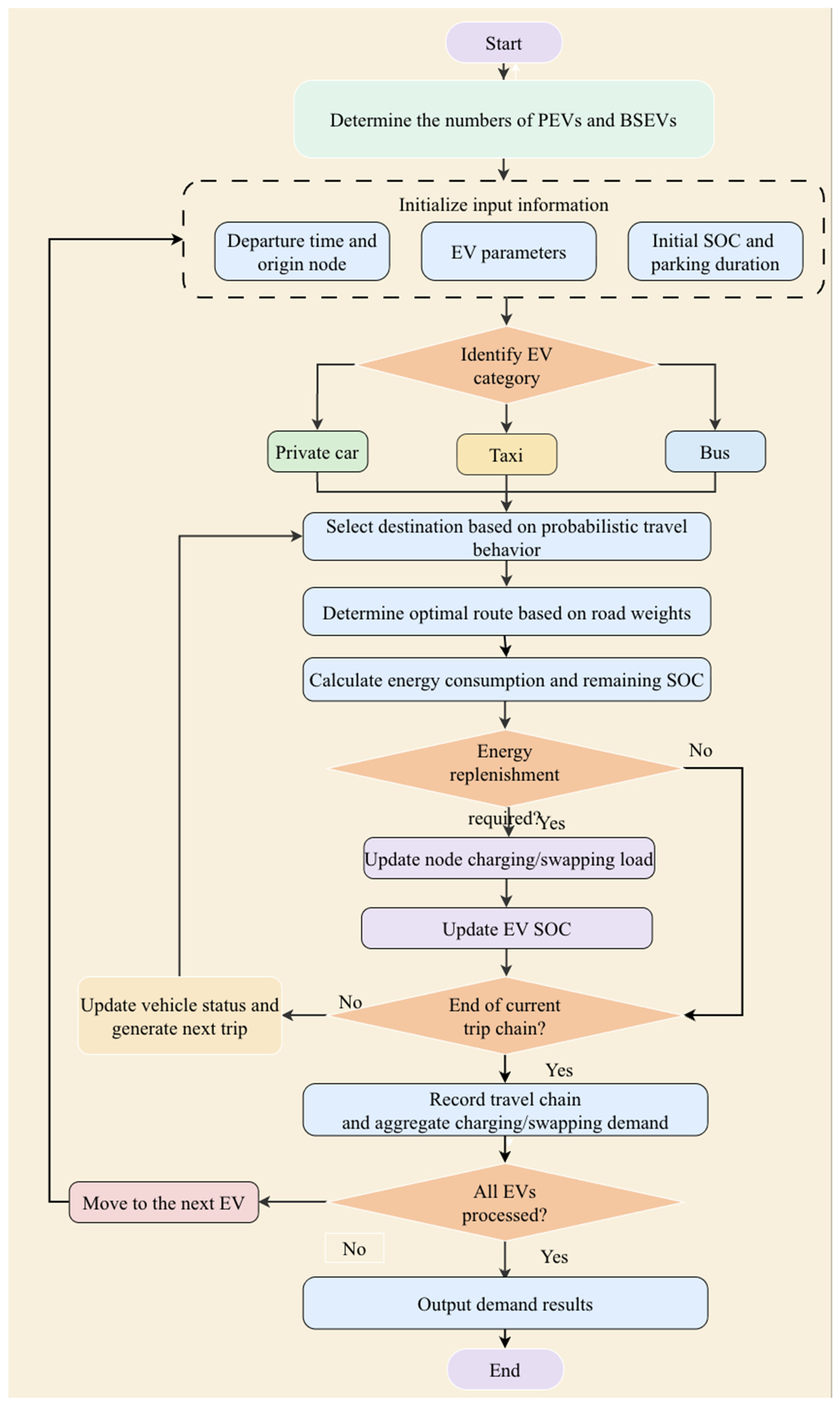
The complete workflow of the proposed charging and swapping demand forecasting model is illustrated in Figure 1.

2.3. Electric-Traffic Coupling Model

The predicted charging and swapping demand in Section 2.2 is obtained at road-network nodes. However, the grid-side impact of EVCS and EVSS depends on the distribution network nodes to which these facilities are connected [44,45]. Therefore, an electric-traffic coupling model is required to map the road-network nodes to the corresponding power-grid nodes. The traffic–grid coupling strategy adopted in this study follows the established coupling framework in [40], in which the association between the transportation network and the distribution network is determined by considering their spatial relationship and the available grid-side capacity. This treatment aims to establish an engineering-feasible correspondence between the two heterogeneous networks while avoiding unreasonable connections between high-demand traffic nodes and heavily loaded grid nodes.

2.3.1. Spatial Coupling Principle

A charging or battery-swapping station located at a road node is generally expected to be connected to a nearby grid node to reduce connection cost and improve engineering feasibility. Let $\mathrm{i}$ denote a road-network node and $\mathrm{k}$ denote a power-grid node. The geographic distance between road node $\mathrm{i}$ and grid node $\mathrm{k}$ can be calculated as

$$D_{i,k}^{\mathrm{s}\mathrm{p}}=2R_{\mathrm{e}}\mathrm{a}\mathrm{r}\mathrm{c}\mathrm{s}\mathrm{i}\mathrm{n}\left[\sqrt{{\mathrm{s}\mathrm{i}\mathrm{n}}^2\left({\displaystyle \frac{\Delta {\phi }_{i,k}}{2}}\right)+\mathrm{c}\mathrm{o}\mathrm{s}\left({\phi }_i\right)\mathrm{c}\mathrm{o}\mathrm{s}\left({\phi }_k\right){\mathrm{s}\mathrm{i}\mathrm{n}}^2\left({\displaystyle \frac{\Delta {\psi }_{i,k}}{2}}\right)}\right]$$

(22)

$$\Delta {\phi }_{i,k}={\phi }_i-{\phi }_k$$

(23)

$$\Delta {\psi }_{i,k}={\psi }_i-{\psi }_k$$

(24)

where ${\mathcal{N}}^{\mathrm{R}}$ and ${\mathcal{N}}^{\mathrm{G}}$ are the sets of road nodes and grid nodes, respectively; $D_{i,k}^{\mathrm{s}\mathrm{p}}$ is the spatial distance index; $R_{\mathrm{e}}$ is the equatorial radius of the Earth; ${\phi }_i$ and ${\phi }_k$ are the latitudes of road node $i$ and grid node $k$, respectively; ${\psi }_i$ and ${\psi }_k$ are the corresponding longitudes; and $\Delta {\phi }_{i,k}$ and $\Delta {\psi }_{i,k}$ are the latitude and longitude differences between the two nodes, respectively.

2.3.2. Capacity Surplus Principle

For grid-side evaluation, the energy replenishment demand obtained in Section 2.2 is converted into an equivalent average power according to the duration of the corresponding time interval. The capacity surplus index is introduced to describe whether grid node $k$ has sufficient remaining capacity to accommodate the charging or swapping load transferred from road node $i$. It is expressed as

$$D_{i,k}^{\mathrm{c}\mathrm{a}\mathrm{p}}=1-{\displaystyle \frac{P_k^{\mathrm{b}\mathrm{a}\mathrm{s}\mathrm{e}}+\underset{t\in \mathcal{T}}{\mathrm{m}\mathrm{a}\mathrm{x}}{P}_i^{\mathrm{d}\mathrm{e}\mathrm{m}}\left(t\right)}{P_k^{\mathrm{m}\mathrm{a}\mathrm{x}}}}$$

(25)

where $P_k^{\mathrm{b}\mathrm{a}\mathrm{s}\mathrm{e}}$ is the basic load of grid node $k$; $P_k^{\mathrm{m}\mathrm{a}\mathrm{x}}$ is the maximum allowable power; $P_i^{\mathrm{d}\mathrm{e}\mathrm{m}}\left(t\right)$ denotes the equivalent average power corresponding to the energy replenishment demand at road node $i$ during time interval $t$. The total equivalent power demand consists of the EVCS and EVSS components:

$$P_i^{\mathrm{d}\mathrm{e}\mathrm{m}}\left(t\right)=P_{i,\mathrm{E}\mathrm{V}\mathrm{C}\mathrm{S}}^{\mathrm{d}\mathrm{e}\mathrm{m}}\left(t\right)+P_{i,\mathrm{E}\mathrm{V}\mathrm{S}\mathrm{S}}^{\mathrm{d}\mathrm{e}\mathrm{m}}\left(t\right)$$

(26)

where $P_{i,\mathrm{E}\mathrm{V}\mathrm{C}\mathrm{S}}^{\mathrm{d}\mathrm{e}\mathrm{m}}\left(t\right)$ and $P_{i,\mathrm{E}\mathrm{V}\mathrm{S}\mathrm{S}}^{\mathrm{d}\mathrm{e}\mathrm{m}}\left(t\right)$ denote the equivalent charging and swapping power demands at road node $i$ during time interval $t$, respectively.

2.3.3. Node Importance Principle

In addition to spatial distance and capacity margin, node importance is introduced to avoid directly coupling high-load traffic nodes with critical or heavily loaded grid nodes. For the power grid, the mean value of the basic load over all grid nodes can be calculated as

$${\mu }^{\mathrm{G}}={\displaystyle \frac{1}{N^{\mathrm{G}}}}{\displaystyle \sum _{k=1}^{N^{\mathrm{G}}}}{P}_k^{\mathrm{b}\mathrm{a}\mathrm{s}\mathrm{e}}$$

(27)

and the standard deviation of the basic load is

$${\sigma }^{\mathrm{G}}=\sqrt{{\displaystyle \frac{1}{N^{\mathrm{G}}}}{\displaystyle \sum _{k=1}^{N^{\mathrm{G}}}}{\left(P_k^{\mathrm{b}\mathrm{a}\mathrm{s}\mathrm{e}}-{\mu }^{\mathrm{G}}\right)}^2}$$

(28)

where $N^{\mathrm{G}}$ is the total number of grid nodes. According to the basic load level, the importance grade of grid node $k$ is defined as

$$G_k^{\mathrm{G}}=\left\{\begin{array}{ll}\mathrm{h}\mathrm{i}\mathrm{g}\mathrm{h},& P_k^{\mathrm{b}\mathrm{a}\mathrm{s}\mathrm{e}}>{\mu }^{\mathrm{G}}+{\sigma }^{\mathrm{G}}\\ \mathrm{m}\mathrm{e}\mathrm{d}\mathrm{i}\mathrm{u}\mathrm{m},& {\mu }^{\mathrm{G}}+{\sigma }^{\mathrm{G}}\ge P_k^{\mathrm{b}\mathrm{a}\mathrm{s}\mathrm{e}}>0\\ \mathrm{l}\mathrm{o}\mathrm{w},& P_k^{\mathrm{b}\mathrm{a}\mathrm{s}\mathrm{e}}=0\end{array}\right.$$

(29)

where $G_k^{\mathrm{G}}$ represents the importance grade of grid node $k$.

The importance of each road node is evaluated according to the average predicted energy replenishment demand. The mean demand of road nodes is expressed as

$${\mu }^{\mathrm{R}}={\displaystyle \frac{1}{N^{\mathrm{R}}}}{\displaystyle \sum _{i=1}^{N^{\mathrm{R}}}}{\displaystyle \frac{1}{T}}{\displaystyle \sum _{t=1}^T}{P}_i^{\mathrm{d}\mathrm{e}\mathrm{m}}\left(t\right)$$

(30)

and the standard deviation is

$${\sigma }^{\mathrm{R}}=\sqrt{{\displaystyle \frac{1}{N^{\mathrm{R}}}}{\displaystyle \sum _{i=1}^{N^{\mathrm{R}}}}{\left({\displaystyle \frac{1}{T}}{\displaystyle \sum _{t=1}^T}{P}_i^{\mathrm{d}\mathrm{e}\mathrm{m}}\left(t\right)-{\mu }^{\mathrm{R}}\right)}^2}$$

(31)

where $N^{\mathrm{R}}$ is the total number of road nodes; $T$ is the number of time intervals. The importance grade of road node $i$ is defined as

$$G_i^{\mathrm{R}}=\left\{\begin{array}{ll}\mathrm{h}\mathrm{i}\mathrm{g}\mathrm{h},& {\displaystyle \frac{1}{T}}{\displaystyle \sum _{t=1}^T}{P}_i^{\mathrm{d}\mathrm{e}\mathrm{m}}\left(t\right)>{\mu }^{\mathrm{R}}+{\sigma }^{\mathrm{R}}\\ \mathrm{m}\mathrm{e}\mathrm{d}\mathrm{i}\mathrm{u}\mathrm{m},& {\mu }^{\mathrm{R}}+{\sigma }^{\mathrm{R}}\ge {\displaystyle \frac{1}{T}}{\displaystyle \sum _{t=1}^T}{P}_i^{\mathrm{d}\mathrm{e}\mathrm{m}}\left(t\right)\ge {\mu }^{\mathrm{R}}-{\sigma }^{\mathrm{R}}\\ \mathrm{l}\mathrm{o}\mathrm{w},& {\displaystyle \frac{1}{T}}{\displaystyle \sum _{t=1}^T}{P}_i^{\mathrm{d}\mathrm{e}\mathrm{m}}\left(t\right)<{\mu }^{\mathrm{R}}-{\sigma }^{\mathrm{R}}\end{array}\right.$$

(32)

where $G_i^{\mathrm{R}}$ represents the importance grade of road node $i$.

2.3.4. Coupling Coefficient and Load Mapping

Based on the above principles, a comprehensive coupling coefficient is constructed to determine the association between road-network nodes and grid nodes. The coefficient combines the spatial distance index and the capacity surplus index:

$${\Gamma }_{i,k}={\beta }_{\mathrm{s}\mathrm{p}}{D}_{i,k}^{\mathrm{s}\mathrm{p}}-{\beta }_{\mathrm{c}\mathrm{a}\mathrm{p}}{D}_{i,k}^{\mathrm{c}\mathrm{a}\mathrm{p}}$$

(33)

where ${\Gamma }_{i,k}$ is the electric-traffic coupling coefficient between road node $i$ and grid node $k$; ${\beta }_{\mathrm{s}\mathrm{p}}$ and ${\beta }_{\mathrm{c}\mathrm{a}\mathrm{p}}$ are the weighting factors of spatial distance and capacity surplus, respectively.

For each road node $i$, the coupled grid node is first selected as the candidate coupled node by minimizing the coupling coefficient:

$$k_i^{*}=\mathrm{a}\mathrm{r}\mathrm{g}\underset{k\in {\mathcal{N}}^{\mathrm{G}}}{\mathrm{m}\mathrm{i}\mathrm{n}}{\Gamma }_{i,k}$$

(34)

The node-importance criterion defined in Section 2.3.3 is then applied as an additional screening condition. Road and grid nodes with simultaneously high importance grades are not allowed to be directly coupled; in such cases, the next eligible grid node according to the coupling coefficient is selected.

After the coupling relationship is determined, the charging and swapping loads generated at road node $i$ are mapped to the corresponding grid node $k_i^{*}$. The total EVCS and EVSS loads connected to grid node $k$ at time $t$ are given by

$$P_{k,\mathrm{E}\mathrm{V}\mathrm{C}\mathrm{S}}\left(t\right)=\sum _{i\in {\mathcal{N}}^{\mathrm{R}}}{\lambda }_{i,k}{P}_{i,\mathrm{E}\mathrm{V}\mathrm{C}\mathrm{S}}^{\mathrm{d}\mathrm{e}\mathrm{m}}\left(t\right)$$

(35)

$$P_{k,\mathrm{E}\mathrm{V}\mathrm{S}\mathrm{S}}\left(t\right)=\sum _{i\in {\mathcal{N}}^{\mathrm{R}}}{\lambda }_{i,k}{P}_{i,\mathrm{E}\mathrm{V}\mathrm{S}\mathrm{S}}^{\mathrm{d}\mathrm{e}\mathrm{m}}\left(t\right)$$

(36)

$${\lambda }_{i,k}=\left\{\begin{array}{c}0,k\ne k_i^{*} \\ 1,k=k_i^{*} \end{array}\right.$$

(37)

where $P_{k,\mathrm{E}\mathrm{V}\mathrm{C}\mathrm{S}}\left(t\right)$ and $P_{k,\mathrm{E}\mathrm{V}\mathrm{S}\mathrm{S}}\left(t\right)$ are the EVCS and EVSS loads connected to grid node $k$, respectively.

Through the electric-traffic coupling model, the road-side charging and swapping demand is transformed into grid-side nodal loads. It should be clarified that the purpose of this coupling model is to provide a physically and operationally reasonable mapping for the subsequent joint planning problem, rather than to formulate the road-to-grid association itself as an additional combinatorial optimization problem. Therefore, the present study does not claim that the resulting mapping represents the theoretical global optimum among all possible road–grid connection combinations. Incorporating the coupling relationship itself into the joint optimization variables could provide a more flexible representation for highly complex network topologies and will be considered in future work.

2.4. Joint Location and Capacity Optimization

The planning model considers three types of stakeholders: infrastructure investors, EV users, and the distribution network. The planning variables include the locations of EVCS and EVSS, the capacities of EVCS, the numbers of fast and slow charging piles, the numbers of batteries in EVSS, and the corresponding grid-connected nodes.

2.4.1. Objective Functions

• Annual construction cost

The first objective is to minimize the annual construction and operation cost of EVCS and EVSS, which is expressed as

$$\mathrm{m}\mathrm{i}\mathrm{n}{F}_1=C_{\mathrm{E}\mathrm{V}\mathrm{C}\mathrm{S}}+C_{\mathrm{E}\mathrm{V}\mathrm{S}\mathrm{S}}$$

(38)

where $C_{\mathrm{E}\mathrm{V}\mathrm{C}\mathrm{S}}$ and $C_{\mathrm{E}\mathrm{V}\mathrm{S}\mathrm{S}}$ are the annual costs of EVCS and EVSS, respectively.

For EVCS, the annual cost is composed of land purchase cost, construction cost, and operation cost:

$$C_{\mathrm{E}\mathrm{V}\mathrm{C}\mathrm{S}}={\displaystyle \sum _{b=1}^{N_{\mathrm{E}\mathrm{V}\mathrm{C}\mathrm{S}}}}\left(C_{b,\mathrm{l}\mathrm{a}}^{\mathrm{E}\mathrm{V}\mathrm{C}\mathrm{S}}+C_{b,\mathrm{c}\mathrm{o}}^{\mathrm{E}\mathrm{V}\mathrm{C}\mathrm{S}}+C_{b,\mathrm{o}\mathrm{p}}^{\mathrm{E}\mathrm{V}\mathrm{C}\mathrm{S}}\right){\displaystyle \frac{r_0{\left(1+r_0\right)}^Y}{{\left(1+r_0\right)}^Y-1}}$$

(39)

$$\left\{\begin{array}{l}{C}_{b,\mathrm{l}\mathrm{a}}^{\mathrm{E}\mathrm{V}\mathrm{C}\mathrm{S}}=x_{b,\mathrm{l}\mathrm{a}}\left({\psi }_f{n}_{b,f}+{\psi }_s{n}_{b,s}+{\psi }_o{n}_{b,o}\right)\\ C_{b,\mathrm{c}\mathrm{o}}^{\mathrm{E}\mathrm{V}\mathrm{C}\mathrm{S}}=x_f{n}_{b,f}+x_s{n}_{b,s}+{\xi }_{\mathrm{c}\mathrm{o}}{J}_b^{\mathrm{E}\mathrm{V}\mathrm{C}\mathrm{S}}\\ C_{b,\mathrm{o}\mathrm{p}}^{\mathrm{E}\mathrm{V}\mathrm{C}\mathrm{S}}=\left(C_{\mathrm{l}\mathrm{a}}^{\mathrm{E}\mathrm{V}\mathrm{C}\mathrm{S}}+C_{\mathrm{c}\mathrm{n}}^{\mathrm{E}\mathrm{V}\mathrm{C}\mathrm{S}}\right)T_b^{\mathrm{E}\mathrm{V}\mathrm{C}\mathrm{S}}+{\xi }_{\mathrm{l}\mathrm{o}}{J}_b^{\mathrm{E}\mathrm{V}\mathrm{C}\mathrm{S}}\end{array}\right.$$

(40)

where $N_{\mathrm{E}\mathrm{V}\mathrm{C}\mathrm{S}}$ is the number of EVCS; $r_0$ is the discount rate; $Y$ is the service life; $x_{b,\mathrm{l}\mathrm{a}}$ is the land price of EVCS $b$; $n_{b,f}$, $n_{b,s}$, and $n_{b,o}$ are the numbers of fast charging piles, slow charging piles, and auxiliary facilities, respectively; ${\psi }_f$, ${\psi }_s$, and ${\psi }_o$ are the corresponding area coefficients; $x_f$ and $x_s$ are the unit prices of fast and slow charging piles, respectively; $J_b^{\mathrm{E}\mathrm{V}\mathrm{C}\mathrm{S}}$ is the capacity of EVCS $b$; ${\xi }_{\mathrm{c}\mathrm{o}}$ and ${\xi }_{\mathrm{l}\mathrm{o}}$ are the construction and loss coefficients, respectively; $C_{\mathrm{l}\mathrm{a}}^{\mathrm{E}\mathrm{V}\mathrm{C}\mathrm{S}}$ and $C_{\mathrm{c}\mathrm{n}}^{\mathrm{E}\mathrm{V}\mathrm{C}\mathrm{S}}$ are the labor and connection costs, respectively; $T_b^{\mathrm{E}\mathrm{V}\mathrm{C}\mathrm{S}}$ is the average operating time.

For EVSS, the annual cost is given by

$$C_{\mathrm{E}\mathrm{V}\mathrm{S}\mathrm{S}}={\displaystyle \sum _{c=1}^{N_{\mathrm{E}\mathrm{V}\mathrm{S}\mathrm{S}}}}\left(C_{c,\mathrm{l}\mathrm{a}}^{\mathrm{E}\mathrm{V}\mathrm{S}\mathrm{S}}+C_{c,\mathrm{c}\mathrm{o}}^{\mathrm{E}\mathrm{V}\mathrm{S}\mathrm{S}}+C_{c,\mathrm{o}\mathrm{p}}^{\mathrm{E}\mathrm{V}\mathrm{S}\mathrm{S}}\right){\displaystyle \frac{r_0{\left(1+r_0\right)}^Y}{{\left(1+r_0\right)}^Y-1}}$$

(41)

$$\left\{\begin{array}{l}{C}_{c,\mathrm{l}\mathrm{a}}^{\mathrm{E}\mathrm{V}\mathrm{S}\mathrm{S}}=A_c^{\mathrm{E}\mathrm{V}\mathrm{S}\mathrm{S}}{x}_{c,\mathrm{l}\mathrm{a}}\\ C_{c,\mathrm{c}\mathrm{o}}^{\mathrm{E}\mathrm{V}\mathrm{S}\mathrm{S}}={\xi }_{\mathrm{i}\mathrm{n}\mathrm{s}}{A}_c^{\mathrm{E}\mathrm{V}\mathrm{S}\mathrm{S}}+{\xi }_{\mathrm{a}\mathrm{r}\mathrm{m}}{N}_{c,\mathrm{a}\mathrm{r}\mathrm{m}}+{\xi }_{\mathrm{b}\mathrm{a}\mathrm{t}}{N}_{c,\mathrm{B}}{J}_{\mathrm{B}}\\ C_{c,\mathrm{o}\mathrm{p}}^{\mathrm{E}\mathrm{V}\mathrm{S}\mathrm{S}}=\left(C_{\mathrm{l}\mathrm{a}}^{\mathrm{E}\mathrm{V}\mathrm{S}\mathrm{S}}+C_{\mathrm{c}\mathrm{n}}^{\mathrm{E}\mathrm{V}\mathrm{S}\mathrm{S}}\right)T_c^{\mathrm{E}\mathrm{V}\mathrm{S}\mathrm{S}}+{\xi }_{\mathrm{B}}{N}_{c,\mathrm{B}}{J}_{\mathrm{B}}\end{array}\right.$$

(42)

where $N_{\mathrm{E}\mathrm{V}\mathrm{S}\mathrm{S}}$ denotes the number of EVSS; $A_c^{\mathrm{E}\mathrm{V}\mathrm{S}\mathrm{S}}$ is the occupied area of EVSS $c$; $x_{c,\mathrm{l}\mathrm{a}}$ is the corresponding land price; $N_{c,\mathrm{a}\mathrm{r}\mathrm{m}}$ and $N_{c,\mathrm{B}}$ are the numbers of mechanical arms and batteries, respectively; $J_{\mathrm{B}}$ is the capacity of a single battery; ${\xi }_{\mathrm{i}\mathrm{n}\mathrm{s}}$, ${\xi }_{\mathrm{a}\mathrm{r}\mathrm{m}}$, ${\xi }_{\mathrm{b}\mathrm{a}\mathrm{t}}$, and ${\xi }_{\mathrm{B}}$ are the installation, mechanical arm, battery investment, and battery operation coefficients, respectively; $C_{\mathrm{l}\mathrm{a}}^{\mathrm{E}\mathrm{V}\mathrm{S}\mathrm{S}}$ and $C_{\mathrm{c}\mathrm{n}}^{\mathrm{E}\mathrm{V}\mathrm{S}\mathrm{S}}$ are the labor and connection costs, respectively; $T_c^{\mathrm{E}\mathrm{V}\mathrm{S}\mathrm{S}}$ is the average operating time.

2.

User satisfaction

The second objective is to maximize user satisfaction. Considering the effects of queuing time and driving time, the satisfaction objective can be calculated as

$$\mathrm{m}\mathrm{a}\mathrm{x}{F}_2=f_{\mathrm{s}\mathrm{a}\mathrm{t}}={\alpha }_w{f}_w\left(t_w\right)+{\alpha }_d{f}_d\left(t_d\right)$$

(43)

where $f_{\mathrm{s}\mathrm{a}\mathrm{t}}$ is the comprehensive satisfaction; $f_w\left(t_w\right)$ and $f_d\left(t_d\right)$ are the waiting satisfaction and driving satisfaction, respectively; $t_w$ and $t_d$ are the waiting time and driving time, respectively; ${\alpha }_w$ and ${\alpha }_d$ are the corresponding weighting coefficients. The functional forms and parameter settings of the waiting satisfaction $f_w\left(t_w\right)$ and driving satisfaction $f_d\left(t_d\right)$ adopted in this study follow those reported in [40], where their detailed formulations are provided. For consistency with the minimization framework of the multi-objective algorithm, the user-oriented objective is implemented as user dissatisfaction, defined as $1-f_{\mathrm{s}\mathrm{a}\mathrm{t}}$. For ease of interpretation, the corresponding user satisfaction is reported in the numerical results.

3.

Voltage fluctuation

The third objective is to minimize voltage fluctuation after the charging and swapping loads are connected to the distribution network:

$$\mathrm{m}\mathrm{i}\mathrm{n}{F}_3={\displaystyle \sum _{k=1}^{N_{\mathrm{g}\mathrm{r}\mathrm{i}\mathrm{d}}}}{\displaystyle \sum _{t=1}^T}\left|V_k\left(t\right)-\overline{V}\right|$$

(44)

where $V_k\left(t\right)$ is the voltage of grid node $k$ at time $t$; $\overline{V}$ is the average voltage of the distribution network; $N_{\mathrm{g}\mathrm{r}\mathrm{i}\mathrm{d}}$ is the number of grid nodes; $T$ is the number of time intervals.

The voltage objective and voltage constraints play complementary roles. The voltage constraints ensure that all nodal voltages remain within the allowable operating range, whereas the voltage objective further minimizes nodal voltage dispersion within the feasible region. Thus, the constraints guarantee operational feasibility, while the objective improves voltage performance among feasible planning schemes.

2.4.2. Constraints

The following constraints are introduced to ensure that the obtained EVCS–EVSS planning scheme is feasible from the perspectives of spatial deployment, service capability, user service quality, and distribution-network operation.

• Distance constraints of charging and swapping facilities

To avoid excessive concentration or unreasonable dispersion of charging and swapping facilities, the distance between any two EVCSs and the distance between any two EVSSs should satisfy the corresponding limits:

$$\left\{\begin{array}{l}{D}_{\mathrm{m}\mathrm{i}\mathrm{n}}^{\mathrm{E}\mathrm{V}\mathrm{C}\mathrm{S}}<D_{b,b^{\prime }}^{\mathrm{E}\mathrm{V}\mathrm{C}\mathrm{S}}<D_{\mathrm{m}\mathrm{a}\mathrm{x}}^{\mathrm{E}\mathrm{V}\mathrm{C}\mathrm{S}}, b\ne b^{\prime }\\ D_{\mathrm{m}\mathrm{i}\mathrm{n}}^{\mathrm{E}\mathrm{V}\mathrm{S}\mathrm{S}}<D_{c,c^{\prime }}^{\mathrm{E}\mathrm{V}\mathrm{S}\mathrm{S}}<D_{\mathrm{m}\mathrm{a}\mathrm{x}}^{\mathrm{E}\mathrm{V}\mathrm{S}\mathrm{S}}, c\ne c^{\prime }\end{array}\right.$$

(45)

where $D_{b,b^{\prime }}^{\mathrm{E}\mathrm{V}\mathrm{C}\mathrm{S}}$ and $D_{c,c^{\prime }}^{\mathrm{E}\mathrm{V}\mathrm{S}\mathrm{S}}$ are the distances between two EVCSs and two EVSSs, respectively; $D_{\mathrm{m}\mathrm{i}\mathrm{n}}^{\mathrm{E}\mathrm{V}\mathrm{C}\mathrm{S}}$, $D_{\mathrm{m}\mathrm{a}\mathrm{x}}^{\mathrm{E}\mathrm{V}\mathrm{C}\mathrm{S}}$, $D_{\mathrm{m}\mathrm{i}\mathrm{n}}^{\mathrm{E}\mathrm{V}\mathrm{S}\mathrm{S}}$, and $D_{\mathrm{m}\mathrm{a}\mathrm{x}}^{\mathrm{E}\mathrm{V}\mathrm{S}\mathrm{S}}$ are the corresponding distance limits.

2.

Capacity constraints

The capacity constraints are introduced to ensure that the planned charging and swapping facilities provide sufficient energy replenishment capability for the predicted demand. Without these constraints, the optimization process may obtain economically favorable but practically infeasible solutions with insufficient service capacity. Therefore, the service capacity of EVCS and EVSS should satisfy the predicted charging and swapping demand:

$$\left\{\begin{array}{l}{\displaystyle \sum _{i=1}^{N_{\mathrm{r}\mathrm{o}\mathrm{a}\mathrm{d}}}}{\displaystyle \sum _{t=1}^T}{P}_{i,\mathrm{E}\mathrm{V}\mathrm{C}\mathrm{S}}^{\mathrm{d}\mathrm{e}\mathrm{m}}\left(t\right)\le {\displaystyle \sum _{b=1}^{N_{\mathrm{E}\mathrm{V}\mathrm{C}\mathrm{S}}}}{J}_b^{\mathrm{E}\mathrm{V}\mathrm{C}\mathrm{S}}\\ {\displaystyle \sum _{i=1}^{N_{\mathrm{r}\mathrm{o}\mathrm{a}\mathrm{d}}}}{\displaystyle \sum _{t=1}^T}{P}_{i,\mathrm{E}\mathrm{V}\mathrm{S}\mathrm{S}}^{\mathrm{d}\mathrm{e}\mathrm{m}}\left(t\right)\le {\displaystyle \sum _{c=1}^{N_{\mathrm{E}\mathrm{V}\mathrm{S}\mathrm{S}}}}{N}_{c,\mathrm{B}}{J}_{\mathrm{B}}\end{array}\right.$$

(46)

where $P_{i,\mathrm{E}\mathrm{V}\mathrm{C}\mathrm{S}}^{\mathrm{d}\mathrm{e}\mathrm{m}}\left(t\right)$ and $P_{i,\mathrm{E}\mathrm{V}\mathrm{S}\mathrm{S}}^{\mathrm{d}\mathrm{e}\mathrm{m}}\left(t\right)$ are the predicted charging demand of PEVs and swapping demand of BSEVs at road node $i$, respectively, $N_{\mathrm{r}\mathrm{o}\mathrm{a}\mathrm{d}}$ is the number of road nodes. The station-specific and time-dependent service-capacity limits are enforced during the demand-allocation process described in Section 2.2.3. Equation (46) therefore provides an additional system-level capacity adequacy requirement.

3.

Power constraints

To ensure the electrical feasibility of EVCS and EVSS integration, nodal power balance should be maintained, and the connected loads should remain within the allowable access limits of the distribution network. The nodal power balance should be maintained as follows:

$${\displaystyle \sum _{k=1}^{N_{\mathrm{g}\mathrm{r}\mathrm{i}\mathrm{d}}}}{\displaystyle \sum _{t=1}^T}\left[P_k^{\mathrm{s}\mathrm{u}\mathrm{p}}\left(t\right)-P_k^{\mathrm{l}\mathrm{o}\mathrm{s}\mathrm{s}}\left(t\right)\right]={\displaystyle \sum _{k=1}^{N_{\mathrm{g}\mathrm{r}\mathrm{i}\mathrm{d}}}}{\displaystyle \sum _{t=1}^T}\left[P_k^{\mathrm{b}\mathrm{a}\mathrm{s}\mathrm{e}}\left(t\right)+P_{k,\mathrm{E}\mathrm{V}\mathrm{C}\mathrm{S}}\left(t\right)+P_{k,\mathrm{E}\mathrm{V}\mathrm{S}\mathrm{S}}\left(t\right)\right]$$

(47)

$$\left\{\begin{array}{l}{P}_{k,\mathrm{E}\mathrm{V}\mathrm{C}\mathrm{S}}\left(t\right)\le P_{k,\mathrm{m}\mathrm{a}\mathrm{x}}^{\mathrm{E}\mathrm{V}\mathrm{C}\mathrm{S}}\\ P_{k,\mathrm{E}\mathrm{V}\mathrm{S}\mathrm{S}}\left(t\right)\le P_{k,\mathrm{m}\mathrm{a}\mathrm{x}}^{\mathrm{E}\mathrm{V}\mathrm{S}\mathrm{S}}\end{array}\right.$$

(48)

where $P_k^{\mathrm{s}\mathrm{u}\mathrm{p}}\left(t\right)$, $P_k^{\mathrm{l}\mathrm{o}\mathrm{s}\mathrm{s}}\left(t\right)$, and $P_k^{\mathrm{b}\mathrm{a}\mathrm{s}\mathrm{e}}\left(t\right)$ are the supplied power, network loss, and base load of grid node $k$, respectively; $P_{k,\mathrm{E}\mathrm{V}\mathrm{C}\mathrm{S}}\left(t\right)$ and $P_{k,\mathrm{E}\mathrm{V}\mathrm{S}\mathrm{S}}\left(t\right)$ are the EVCS and EVSS loads connected to node $k$, respectively; $P_{k,\mathrm{m}\mathrm{a}\mathrm{x}}^{\mathrm{E}\mathrm{V}\mathrm{C}\mathrm{S}}$ and $P_{k,\mathrm{m}\mathrm{a}\mathrm{x}}^{\mathrm{E}\mathrm{V}\mathrm{S}\mathrm{S}}$ are the corresponding access power limits. Equation (47) represents an aggregate system-level power-balance constraint rather than the detailed nodal power-flow equation. The detailed nodal active and reactive power-flow formulations are provided in [40].

4.

Waiting time constraint

To guarantee an acceptable level of user service quality, the waiting time of each EV user should not exceed the maximum allowable queuing time:

$$W_f\le W_{\mathrm{m}\mathrm{a}\mathrm{x}}$$

(49)

where $W_f$ is the waiting time of EV user $f$; $W_{\mathrm{m}\mathrm{a}\mathrm{x}}$ is the maximum acceptable waiting time.

5.

Voltage constraint

The voltage constraint is introduced to maintain secure distribution-network operation after the integration of charging and swapping loads. Large and spatially concentrated EVCS/EVSS loads may cause excessive voltage deviations at weak or heavily loaded nodes. Therefore, the voltage magnitude of each distribution-network node should remain within the allowable operating range:

$$V_{k,\mathrm{m}\mathrm{i}\mathrm{n}}\le V_k\left(t\right)\le V_{k,\mathrm{m}\mathrm{a}\mathrm{x}}$$

(50)

where $V_{k,\mathrm{m}\mathrm{i}\mathrm{n}}$ and $V_{k,\mathrm{m}\mathrm{a}\mathrm{x}}$ are the lower and upper voltage limits of grid node $k$, respectively.

Overall, the proposed optimization model consists of four interconnected components. First, the microscopic transportation-network model and EV travel characteristics are used to determine vehicle trajectories, energy consumption, SOC evolution, and the resulting spatiotemporal charging and swapping demand. Second, the electric–traffic coupling model maps the road-side replenishment demand to the corresponding distribution-network nodes by considering spatial distance, grid-side capacity margin, and node-importance screening. Third, the joint EVCS–EVSS planning model simultaneously determines station locations and capacities under station-deployment, service-capacity, waiting-time, power, and voltage constraints. Finally, the spatiotemporal demand and traffic–grid mapping results are used to evaluate each candidate planning scheme, and annualized infrastructure cost, user dissatisfaction, and voltage fluctuation are jointly optimized to obtain a set of feasible Pareto planning solutions. These components together form the overall structure of the proposed joint location-and-capacity optimization model.

3. Solution Methodology

3.1. Random Forest Surrogate Model

The joint location and capacity planning of EVCSs and EVSSs is formulated as a nonlinear multi-objective optimization problem. During the evolutionary search, each candidate planning scheme must be evaluated in terms of comprehensive annualized cost, user satisfaction, and voltage fluctuation. The cost objective can be calculated directly from the station locations, installed charging piles, battery inventories, land prices, and equipment parameters. By contrast, the evaluation of user satisfaction and voltage fluctuation requires repeated traffic-service analysis, demand allocation, and power-flow calculation. These procedures become computationally intensive when a large number of candidate solutions are evaluated over successive generations.

To improve the optimization efficiency, an RF-based surrogate model is introduced to approximate the computationally intensive objective evaluations. In the proposed framework, the economic cost objective is retained as an exact evaluation, whereas RF models are constructed for the user satisfaction-related objective and voltage fluctuation objective. In addition, considering that infeasible solutions may affect the evolutionary search, an auxiliary RF classifier is introduced to estimate constraint violation probability.

The accuracy of the RF regression models is evaluated using root mean square error (RMSE), mean absolute error (MAE), and $R^2$:

$$\mathrm{R}\mathrm{M}\mathrm{S}\mathrm{E}=\sqrt{{\displaystyle \frac{1}{N}}{\displaystyle \sum _{i=1}^N}{(y_i-{\widehat{y}}_i)}^2}$$

(51)

$$\mathrm{M}\mathrm{A}\mathrm{E}={\displaystyle \frac{1}{N}}\left|y_i-{\widehat{y}}_i\right|$$

(52)

$$R^2=1-{\displaystyle \frac{{\displaystyle {\sum }_{i=1}^N}{\left(y_i-{\widehat{y}}_i\right)}^2}{{\displaystyle {\sum }_{i=1}^N}{\left(y_i-\overline{y}\right)}^2}}$$

(53)

where $y_i$ and ${\widehat{y}}_i$ are the true and predicted values, respectively.

The RF surrogate models are implemented using MATLAB R2025a TreeBagger. Each ensemble contains 100 bagged trees with out-of-bag prediction enabled. The user-dissatisfaction model is trained using all accumulated true-evaluation samples, whereas the voltage-fluctuation model uses only truly feasible samples. The auxiliary feasibility model is implemented as a class-balanced RF model that produces a continuous constraint-violation score. The trained RF models are subsequently embedded into the evolutionary optimization process. Through this strategy, expensive traffic allocation and power-flow calculations are avoided for most candidate solutions, while the original optimization model is retained for periodic correction and final verification.

3.2. RF-SA-NSGA-III Framework

Initially, 300 planning schemes are generated by independent uniform sampling within the prescribed bounds of the 34 decision variables, and the discrete variables are rounded upward before true-model evaluation. After surrogate activation, up to 20 representative solutions are evaluated using the full model every five generations. These solutions include predicted Pareto elites, samples close to the feasibility boundary, predicted feasible solutions with relatively low voltage fluctuation, and decision-space-diverse samples selected using a greedy farthest-point criterion. The newly evaluated true samples are then incorporated into the cumulative training dataset for surrogate updating.

The proposed RF-SA-NSGA-III algorithm retains the basic evolutionary framework of NSGA-III, including nondominated sorting, reference-point-based selection, crossover, and mutation operations. Instead of modifying the evolutionary operators, the proposed method focuses on improving the objective evaluation process.

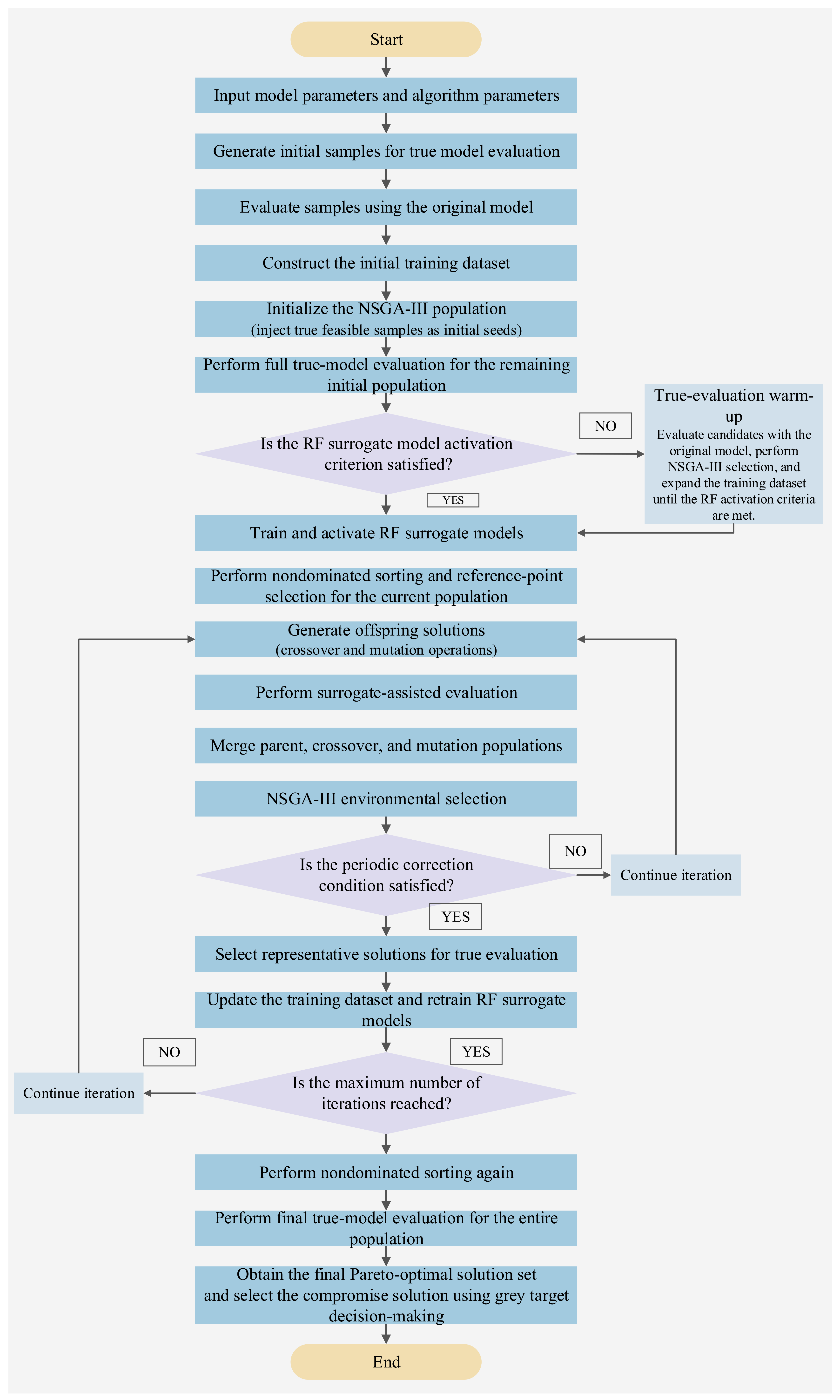
To further improve search reliability, the predicted constraint information is considered during surrogate evaluation. A threshold of 0.5 is used for the predicted constraint-violation score. Solutions classified as infeasible are assigned a penalty value of ${10}^8$ for all three objectives, thereby preventing them from dominating the evolutionary search. The overall procedure of the proposed RF-SA-NSGA-III algorithm is illustrated in Figure 2.

Different from directly accepting surrogate-based results, the proposed final verification eliminates the influence of surrogate prediction errors on the final planning decision. In the implementation, the entire retained population is reevaluated by the original model before the final Pareto front is obtained.

Compared with conventional NSGA-III, the proposed method reduces the number of expensive objective evaluations while maintaining the reliability of the final planning results through continuous surrogate correction and final real-model validation. During optimization, the algorithm records the number of true evaluations, surrogate predictions, training samples, and RF updates to quantitatively analyze the computational efficiency improvement.

To reduce the influence of subjective preferences on the selection of the final solution from the Pareto-optimal set, an improved gray target decision-making (IGTDM) method based on the entropy weight method (EWM) is adopted [46]. The Pareto objective values are first normalized, and the weights of the evaluation criteria are objectively determined according to their information entropy. A gray target decision matrix is then constructed, and the comprehensive target distance of each Pareto solution is evaluated. The solution with the minimum comprehensive target distance is selected as the final compromise solution. The IGTDM procedure is applied only after the Pareto-optimal set has been obtained and therefore does not affect the evolutionary search process or the generation of the Pareto front. Detailed formulations and computational procedures can be found in reference [46].

4. Case Studies

4.1. Case Description and Data Preparation

4.1.1. Case System Description

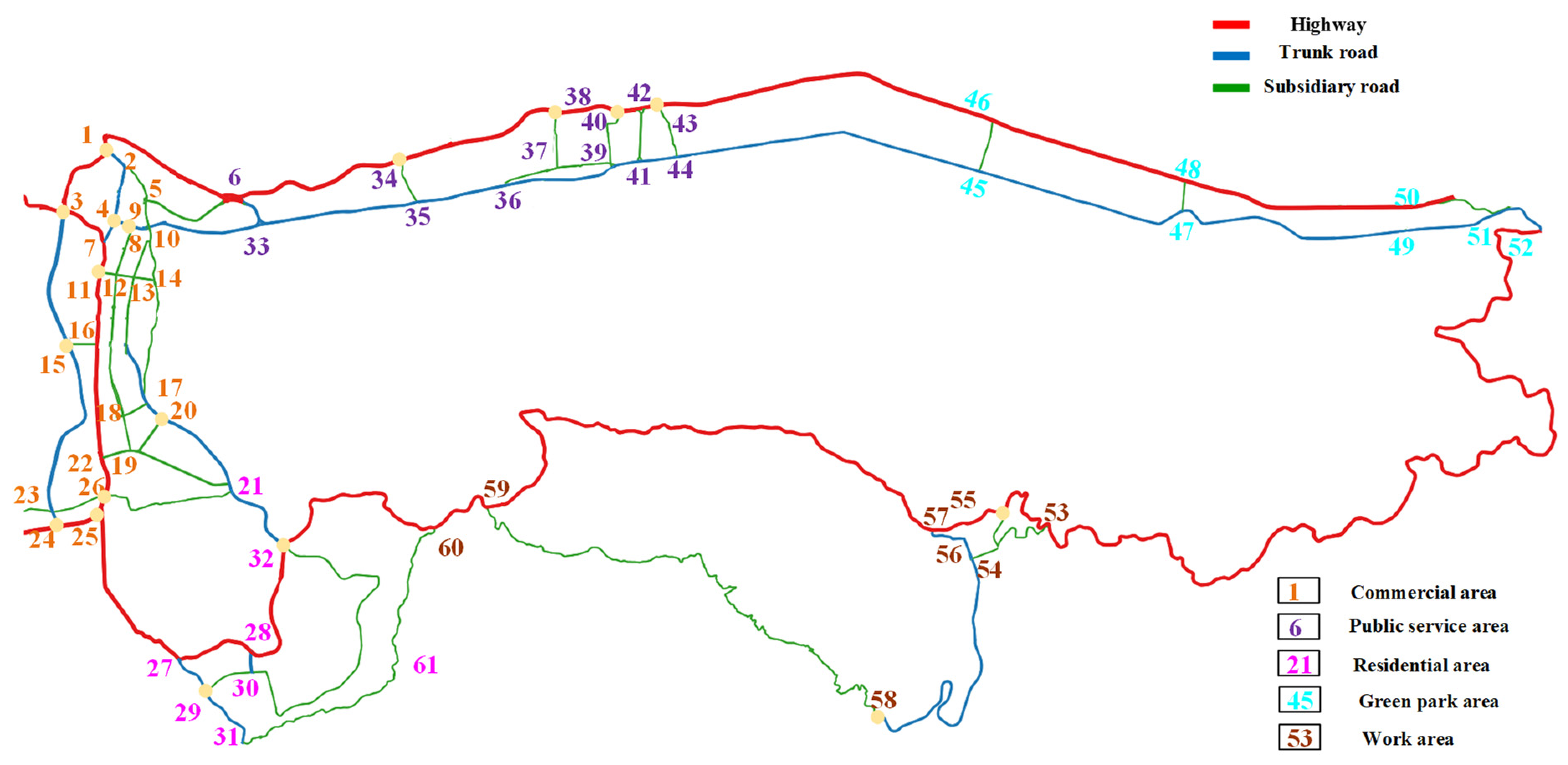
To verify the effectiveness of the proposed method, a simulation case is constructed using an actual urban road network of Dali and the IEEE 69-bus benchmark distribution system. The road network preserves the spatial topology of the studied urban area, while the benchmark distribution system is used to represent the grid-side operating characteristics for planning analysis. The road-node classification is determined based on OpenStreetMap road-network data processed in QGIS, with the study area divided into five functional zones. The topology of the transportation network and classified road nodes are illustrated in Figure 3.

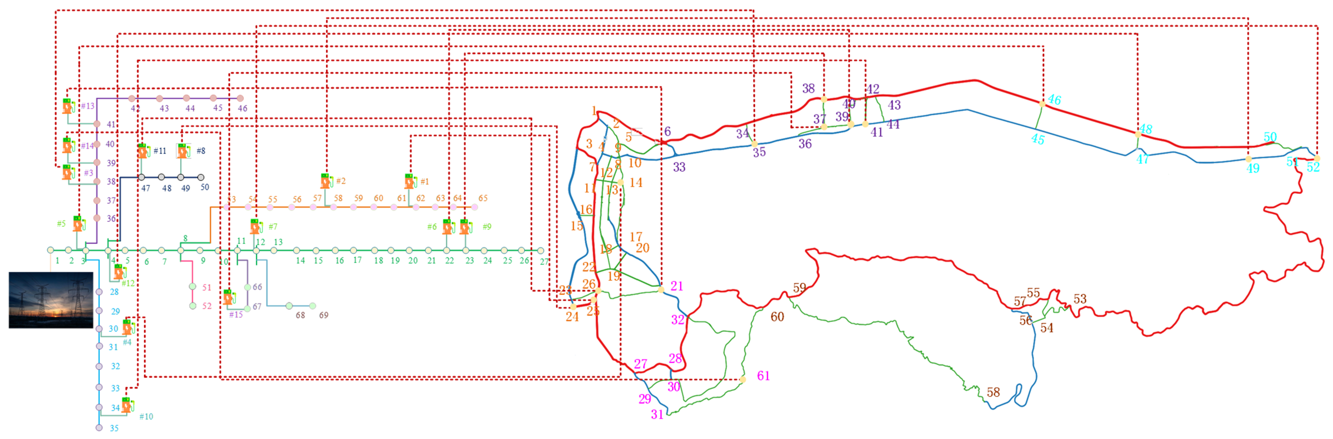
Based on the coupling principle described in Section 2.3, the transportation network and distribution network of the studied area are integrated to establish the traffic-grid coupled system. The road nodes are mapped to the corresponding power network buses, and the resulting coupled topology is illustrated in Figure 4.

4.1.2. Charging Demand Forecasting Results

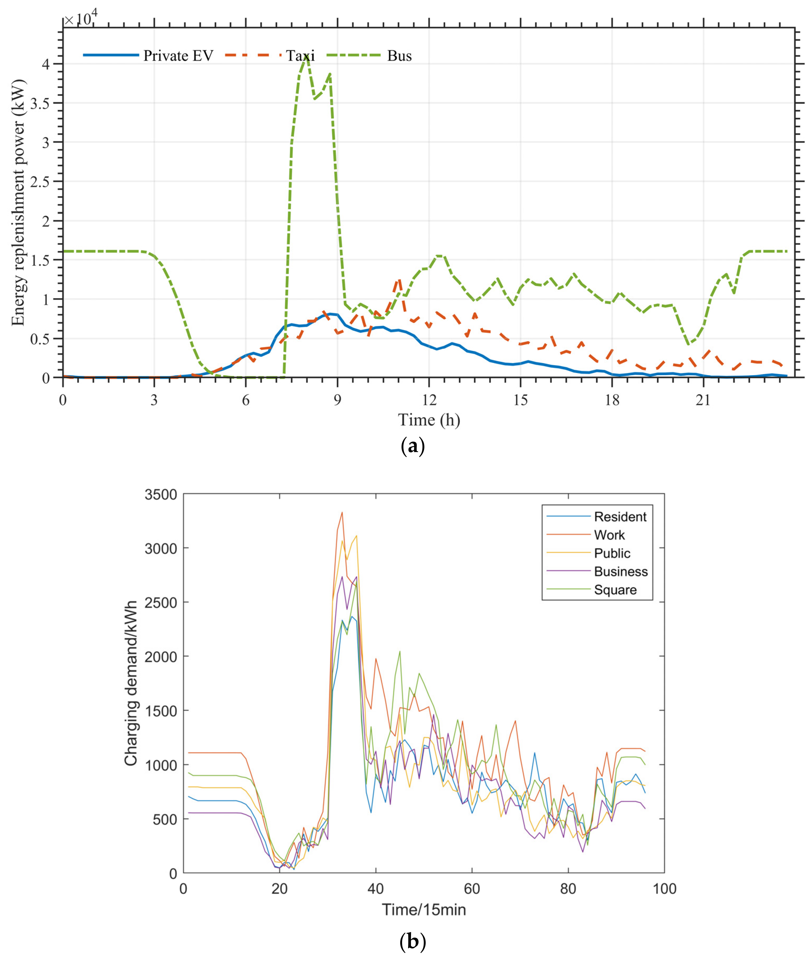
The energy replenishment demand forecasting results are presented in Figure 5 and Figure 6. Figure 5a presents the daily energy replenishment power profiles of private EVs, taxis, and buses. Total daily energy replenishment demand reaches 423.30 MWh, with buses contributing the largest proportion, followed by taxis and private EVs. The demand profiles of different vehicle categories exhibit distinct temporal characteristics. Private EVs mainly concentrate their replenishment demand in the morning period and reach the peak during 08:45–09:00. The battery swapping demand of taxis is distributed over a relatively longer period and reaches its maximum during 11:00–11:15. Compared with private EVs and taxis, buses maintain a higher replenishment demand throughout the day and achieve the maximum demand during 08:00–08:15. The detailed demand statistics of different vehicle categories are provided in

Table 1. Energy replenishment demand statistics of different vehicle categories.

Vehicle Type	Total Number	Number of Vehicles Requiring Replenishment	Replenishment Vehicle Ratio	Daily Energy Replenishment Demand (MWh)	Energy Demand Ratio	Peak Power (MW)	Peak Period
Private EV	2204	704	31.94%	51.52	12.17%	8.09	08:45–09:00
Taxi	1770	1706	96.38%	82.36	19.46%	13.01	11:00–11:15
Bus	1026	974	94.93%	289.42	68.37%	41.29	08:00–08:15

.

Figure 5b presents the energy replenishment demand distribution among different functional areas, including residential, working, commercial, public service, and square areas. The working area has the largest daily demand of 104.57 MWh, accounting for 24.70% of the total demand, followed by the square area with 92.37 MWh. The demand proportions of public service, residential, and commercial areas are 18.90%, 17.56%, and 17.01%, respectively. The demand peaks of all functional areas occur mainly during 08:00–09:00, while the specific peak periods vary among different areas. These differences indicate that energy replenishment demand exhibits clear spatial characteristics associated with different functional areas.

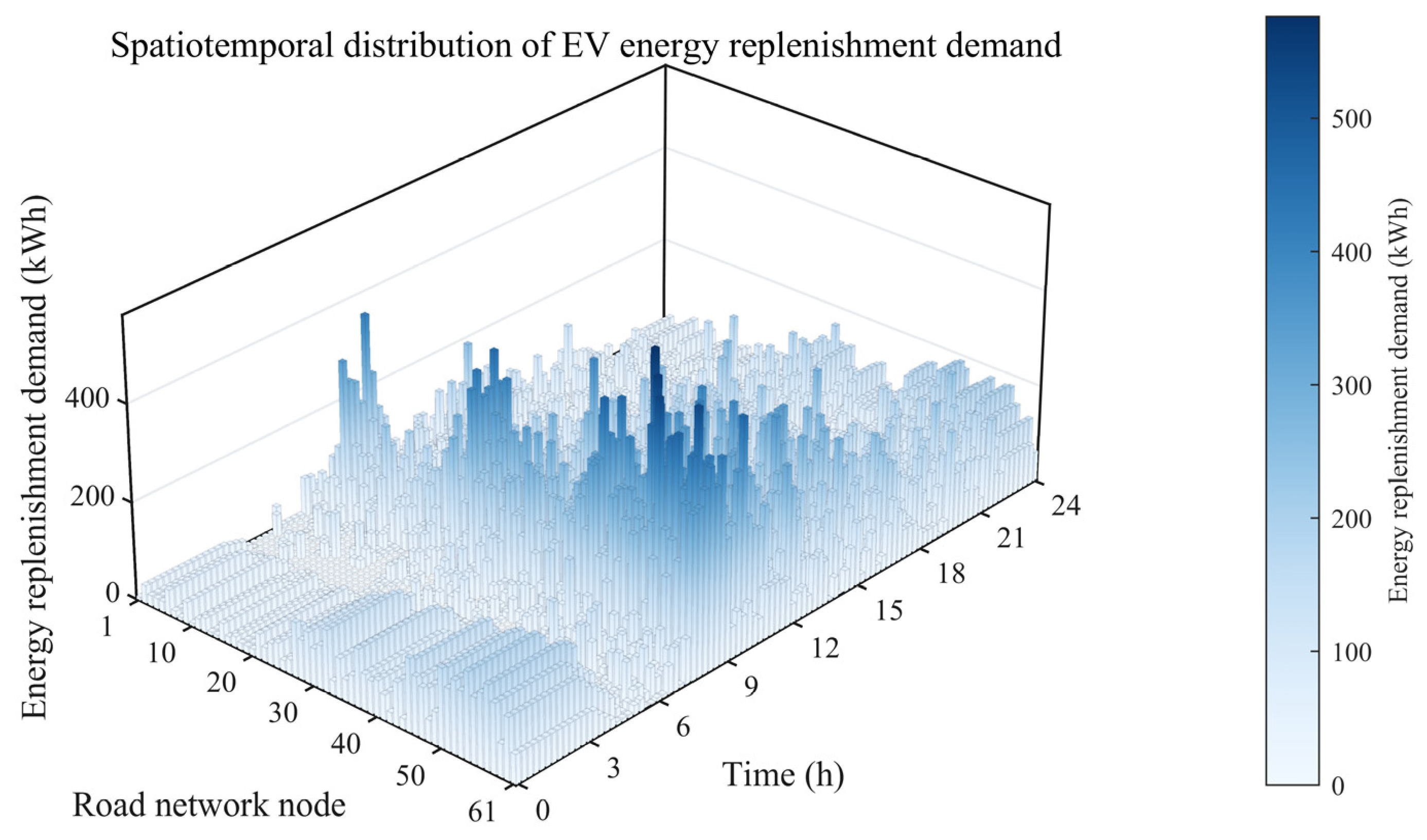
Figure 6 further shows the spatiotemporal distribution of energy replenishment demand across the 61 road network nodes and 96 time intervals. The demand covers all road nodes but presents significant differences in both spatial distribution and temporal variation. A continuous high-demand period appears between 07:45 and 09:00, during which the system reaches the maximum aggregated replenishment load of 55.13 MW at 08:00–08:15. During this peak period, Node 54 has the highest replenishment demand among all nodes. This node is located in a working area and at the intersection of a trunk road and a subsidiary road, which corresponds to its high energy replenishment requirement. Besides Node 54, Nodes 60, 46, 57, and 56 also exhibit relatively high demand levels, forming the major spatial demand clusters during the morning peak period.

4.2. Optimization Results and Algorithm Comparison

4.2.1. Comparison of Optimization Performance

To evaluate the effectiveness of the proposed RF-SA-NSGA-III algorithm, three benchmark algorithms, including MOTEO, NSGA-II, and the standard NSGA-III, are selected for comparative analysis. The optimization performance is evaluated from two aspects: solution quality and computational efficiency. To ensure a consistent comparison, all algorithms are applied to the same EVCS–EVSS planning problem with identical model settings, input data, population size, maximum number of iterations, termination criteria, computational platform, result-statistics procedure, and compromise-solution selection method. Therefore, the algorithms are evaluated under an equivalent evolutionary search budget. The detailed search parameters of different optimization algorithms are listed in

Table 2. Search parameter settings of different optimization algorithms.

Parameter	MOTEO	NSGA-II	NSGA-III	RF-SA-NSGA-III
Population size	100	100	100	100
Maximum number of iterations	200	200	200	200
Crossover probability	0.7	0.7	0.5	0.5
Mutation probability	0.4	0.4	0.5	0.5
Variable mutation rate	0.02	0.02	0.02	0.02

The algorithm-specific crossover and mutation parameters are retained according to commonly adopted configurations for the corresponding search mechanisms rather than being forcibly unified across different algorithms. These settings are intended to provide practical benchmark configurations and are not claimed to be globally optimal. In particular, NSGA-III and RF-SA-NSGA-III use identical evolutionary operators and parameter settings, so that their performance difference mainly reflects the effect of the proposed surrogate-assisted evaluation strategy.

The proposed RF-SA-NSGA-III retains the original evolutionary operators and reference-point mechanism of NSGA-III, while introducing surrogate-assisted evaluation to reduce computational cost. The parameters of the random forest surrogate model adopted in RF-SA-NSGA-III are provided in

Table 3. Parameter settings of the RF surrogate model.

Surrogate Model Parameter	Setting Value	Function
Initial number of true samples	300	Construct the initial random forest training dataset
Surrogate model update interval	5	Perform true-model correction every 5 generations
Number of samples per update	20	Add 20 newly evaluated true samples in each update
Minimum number of training samples	100	Minimum training dataset size required to activate the surrogate model
Minimum number of feasible samples	20	Minimum number of feasible samples required for feasibility model training
Minimum feasible samples for objective 3	50	The voltage fluctuation surrogate model is trained only using true feasible samples
Threshold for activating feasible samples	50	Determined by the larger value between 20 and 50
Minimum number of infeasible samples	20	Ensure sufficient samples for learning the feasibility boundary
Number of trees in random forest	100	Each surrogate model contains 100 regression trees

.

The parameters in Table 3 were selected as practical settings to balance surrogate prediction reliability and the computational cost of true-model evaluations, rather than as globally optimized hyperparameters. In particular, the initial sampling size provides sufficient true-evaluation data for surrogate initialization, while the periodic update interval and number of true evaluations per update balance surrogate correction frequency against computational savings. The RF ensemble size was selected to provide stable prediction performance without introducing excessive training overhead.

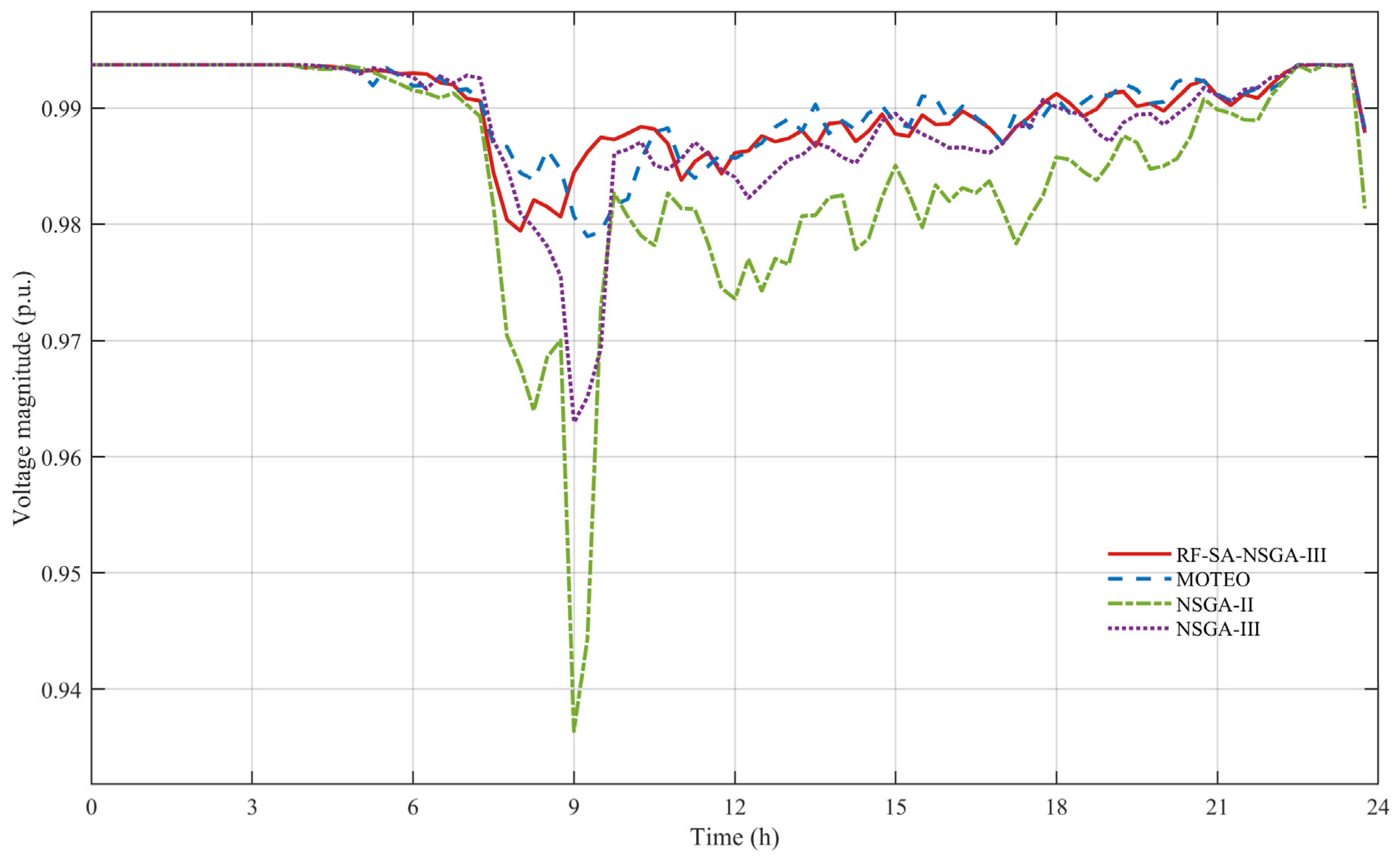
The optimization results of different algorithms are summarized in

Table 4. Optimization results comparison among different algorithms.

Algorithm	Total Annualized Cost (CNY)	User Satisfaction	Voltage Fluctuation
MOTEO	6,944,022.888	0.61830	1.0589
NSGA-II	6,867,567.324	0.62136	2.7329
NSGA-III	7,175,612.393	0.61574	1.6199
RF-SA-NSGA-III	7,079,752.702	0.61252	1.0030

, where the three objective values obtained by each algorithm are compared. In addition, the voltage fluctuation profiles corresponding to the optimal solutions obtained by different algorithms are illustrated in Figure 7 for further comparison.

The results indicate that different algorithms exhibit different optimization characteristics for the multi-objective EVCS–EVSS planning problem. NSGA-II achieves the lowest annualized cost among the compared algorithms, while NSGA-III obtains the highest user satisfaction value. However, both algorithms result in relatively higher voltage fluctuation values, indicating that solutions optimized mainly toward economic or service objectives may negatively affect distribution network operation.

In comparison, RF-SA-NSGA-III achieves the lowest voltage fluctuation value among all algorithms while maintaining comparable user dissatisfaction and annualized cost. Although its annualized cost is slightly higher than those of NSGA-II and MOTEO, the difference remains within an acceptable range, while voltage regulation performance is significantly improved. To complement the voltage profiles shown in Figure 7,

Table 5. Voltage-performance and network-loss indicators for different algorithms.

Algorithms	Minimum System-Average Voltage (p.u.)	Maximum Deviation of System-Average Voltage Profile (p.u.)	Minimum Bus-Average Voltage (p.u.)	Maximum Deviation of Bus-Average Voltage (p.u.)	Active Power Loss of the Distribution Network
MOTEO	0.978924	0.021076	0.972287	0.027713	0.040440
NSGA-II	0.936389	0.063611	0.969376	0.030624	0.116396
NSGA-III	0.962926	0.037074	0.964708	0.035292	0.078450
RF-SA-NSGA-III	0.979422	0.020578	0.975472	0.024528	0.039166

reports several quantitative voltage and network-loss indicators for the optimal solutions obtained by different algorithms.

Overall, the proposed RF-SA-NSGA-III algorithm preserves the optimization capability of the original NSGA-III framework and achieves competitive objective values among different optimization methods. Combined with the subsequent computational efficiency analysis, the proposed method demonstrates that the computational burden can be substantially reduced while maintaining competitive optimization performance for complex EVCS–EVSS planning problems.

To further evaluate the statistical robustness and overall Pareto-front quality of the compared algorithms, hypervolume (HV) and inverted generational distance (IGD) were calculated based on the results of 5 independent runs. The corresponding mean and standard deviation are reported in

Table 6. Statistical performance of different algorithms over independent runs.

Algorithm	HV (Mean ± Std)	IGD (Mean ± Std)
MOTEO	0.579045 ± 0.053544	0.174850 ± 0.022865
NSGA-II	0.540864 ± 0.030861	0.189697 ± 0.018246
NSGA-III	0.600242 ± 0.075338	0.183135 ± 0.025223
RF-SA-NSGA-III	0.694599 ± 0.298682	0.240335 ± 0.054083

, where a larger HV and a smaller IGD indicate better multi-objective optimization performance.

As shown in Table 6, RF-SA-NSGA-III achieved the highest mean HV, indicating its strong ability to obtain high-quality Pareto solutions with a large dominated objective-space volume. However, its relatively large HV standard deviation and higher IGD suggest greater run-to-run variability and less uniform coverage of the empirical reference front. In comparison, MOTEO obtained the lowest mean IGD. These results indicate that RF-SA-NSGA-III provides strong solution quality, while further improvement in robustness and front coverage remains possible.

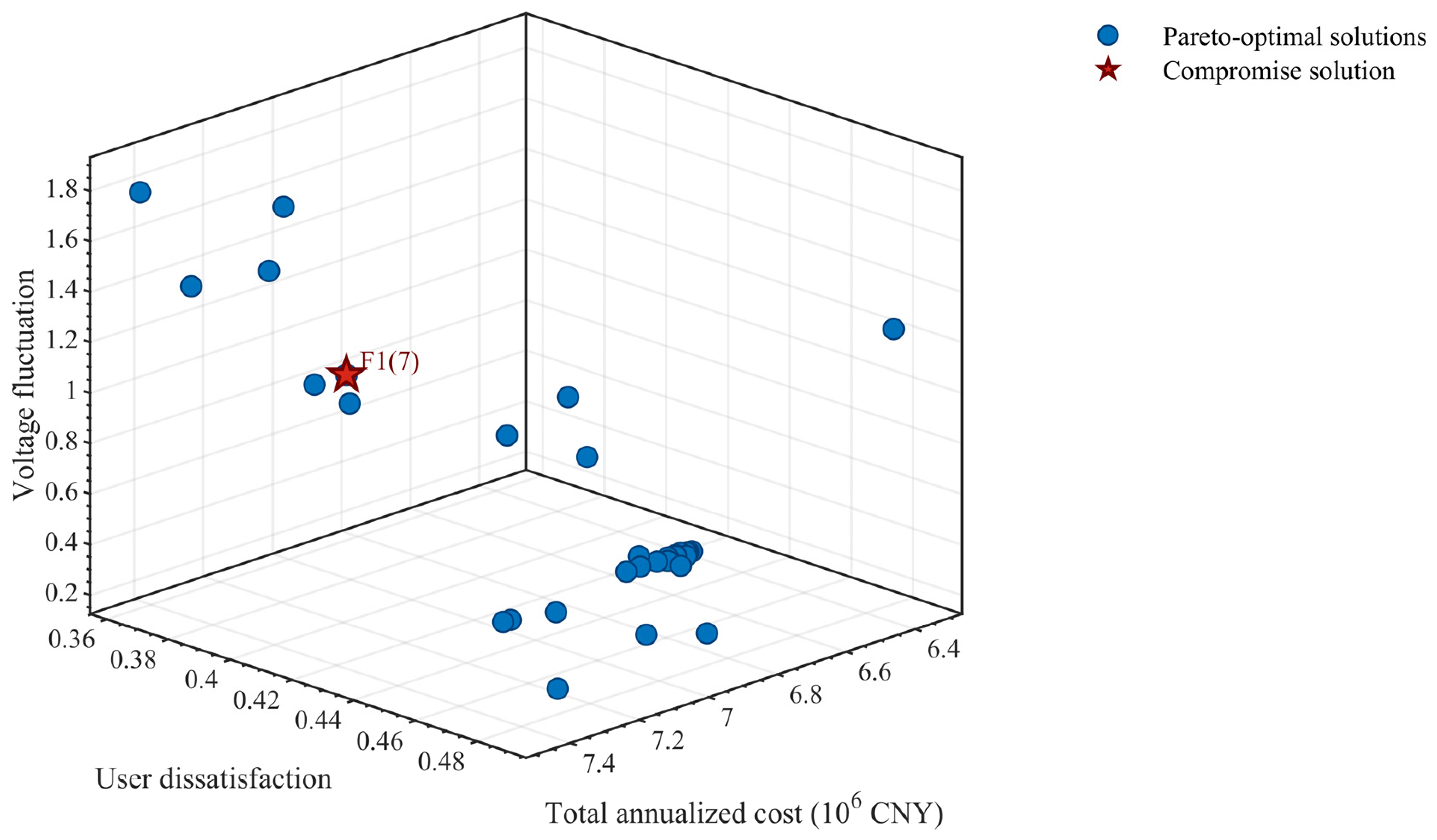
The Pareto optimal solutions obtained by RF-SA-NSGA-III are illustrated in Figure 8. The solution set presents the trade-off relationship among annualized cost, user dissatisfaction, and voltage fluctuation in the three-dimensional objective space. The selected compromise solution F1(7) achieves relatively low voltage fluctuation while maintaining competitive performance in economic cost and user service objectives. The corresponding objective values are consistent with those reported in Table 4.

To further evaluate the computational efficiency of the RF surrogate-assisted strategy, the evaluation statistics of RF-SA-NSGA-III are summarized in

Table 7. Computational efficiency statistics of RF-SA-NSGA-III.

Indicator	Value
Total candidate evaluations	21,258
True objective evaluations	2258
Surrogate-based evaluations	19,000
Surrogate evaluation ratio	89.38%
Final training samples	2040
Training samples/True evaluations	90.35%
Surrogate model updates	39
Computational time (s)	4689.4

. During the 200-generation optimization, a total of 21,258 evaluation calls are recorded, including 2258 full-model evaluations and 19,000 surrogate evaluations, with the latter accounting for 89.38% of the total. Selected surrogate-assessed solutions are reevaluated using the full model during the correction and final verification stages, resulting in a slightly higher total number of evaluation calls. Compared with the approximately 20,100 full-model evaluations required by standard NSGA-III under the same population and iteration settings, RF-SA-NSGA-III reduces the number of computationally expensive full-model evaluations by approximately 88.77%. The final surrogate training dataset contains 2040 true samples, corresponding to 90.35% of the 2258 full-model evaluations, and the surrogate model is updated 39 times during the optimization process. Furthermore, computational time is reduced from 45,706.3 s for standard NSGA-III to 4689.4 s for RF-SA-NSGA-III, corresponding to a reduction of approximately 89.74%. The total runtime of 4689.4 s includes approximately 448.9 s for initial sample generation, 143.5 s for initial population evaluation, 3965.1 s for the main optimization loop, and 131.6 s for final true-model verification. Within the true-objective evaluations, traffic assignment and power-flow calculations require approximately 174.7 s and 3095.3 s, respectively, whereas RF training requires only 11.4 s, indicating that power-flow calculation remains the dominant computational component.

To evaluate the prediction reliability of the random forest surrogate models, MAE, RMSE, and $R^2$ are employed as evaluation metrics. The prediction performance of the surrogate models for objective 2 (user satisfaction) and objective 3 (voltage fluctuation) is summarized in

Table 8. Prediction performance of the RF surrogate models for Objectives 2 and 3.

Surrogate Model	MAE	RMSE	${\mathit{R}}^2$
Objective 2: user satisfaction	0.0182	0.0287	0.7590
Objective 3: voltage fluctuation	0.0971	0.1755	0.8778

.

The reported MAE, RMSE, and $R^2$ values are calculated from out-of-bag predictions of the random forest models using the dynamically accumulated true-evaluation samples collected throughout the optimization process. Objective 2 uses all accumulated true samples, whereas Objective 3 uses only truly feasible samples. For objective 2, the surrogate model achieves a relatively low prediction error and a satisfactory coefficient of determination. The surrogate model can effectively capture the variation trend of this objective and provide reliable guidance for the evolutionary search process. For objective 3, the surrogate model exhibits better fitting performance compared with objective 2. This is mainly attributed to the use of feasible samples for model training and the corresponding data processing strategy, which improves the prediction capability for grid-related objectives. Although a small number of samples may still exhibit relatively larger prediction deviations, the overall prediction results are sufficient to reflect the changing trends of the original objectives. Therefore, the trained surrogate models can provide effective approximate evaluations for RF-SA-NSGA-III and reduce the dependence on repeated true-model calculations.

To further examine the influence of surrogate uncertainty across the Pareto front, an RMSE-based error-band sensitivity analysis was conducted for five representative solutions. Objectives 2 and 3 were independently perturbed by $-RMSE$, 0, and $+RMSE$. As shown in

Table 9. RMSE-based sensitivity analysis of representative solutions across the final Pareto front.

Pareto Region	Solution	Objective 2 Value	Relative RMSE Exposure of Objective 2 (%)	Objective 3 Value	Relative RMSE Exposure of Objective 3 (%)	Nondominated Cases Under RMSE Perturbations
Cost extreme	F1(21)	0.51980	5.97	1.21458	14.45	9/9
User-service extreme	F1(18)	0.63567	7.87	1.80925	9.70	6/9
Voltage extreme	F1(23)	0.51709	5.94	0.25142	69.81	6/9
Middle front	F1(17)	0.54326	6.28	0.41518	42.27	6/9
Final compromise solution	F1(7)	0.61252	7.40	1.00301	17.50	9/9

, the cost-extreme and final compromise solutions remained nondominated under all nine perturbation combinations, whereas the user-service-extreme, voltage-extreme, and middle-front solutions remained nondominated in six cases. The voltage-extreme region showed higher relative sensitivity because of its small baseline objective value. Overall, the final compromise solution exhibits satisfactory local stability at the observed surrogate-error level.

To examine the robustness of RF-SA-NSGA-III to changes in input data, the EV population was varied as a representative input factor, and the corresponding objective values and surrogate-model accuracy metrics are summarized in

Table 10. Sensitivity of optimization performance and surrogate accuracy to EV population.

EV Population	Total Annualized Cost (CNY)	User Satisfaction	Voltage Fluctuation	MAE (Objective2/3)	RMSE (Objective2/3)	${\mathit{R}}^2$(Objective2/3)
4500	5,765,766	0.51979	0.6742	0.0177/0.0878	0.0276/0.1648	0.6287/0.8954
5000	7,079,752	0.61252	1.0030	0.0182/0.0971	0.0287/0.1755	0.7590/0.8778
5500	6,829,928	0.53747	0.8738	0.0157/0.0298	0.0264/0.0745	0.6480/0.8845

.

The sensitivity analysis shows that RF-SA-NSGA-III can consistently obtain feasible planning solutions when the EV population varies by ±10% from the baseline level. The three objective values change with the variation in EV population, reflecting the trade-offs among annualized cost, user satisfaction, and voltage performance under different demand levels. Meanwhile, the surrogate models maintain generally stable prediction accuracy across the three scenarios, with comparable MAE, RMSE, and $R^2$ values. These results indicate that the proposed method retains reasonable adaptability to changes in EV population.

Overall, the RF-SA-NSGA-III algorithm effectively integrates surrogate prediction and true-model correction to accelerate the optimization process of the EVCS–EVSS joint planning problem. The random forest surrogate models are capable of capturing the nonlinear relationship between planning variables and complex objective functions, providing reliable approximate evaluations during the evolutionary search. Although prediction errors inevitably exist in the surrogate-assisted optimization process, the proposed periodic correction mechanism, dynamic training dataset updating, and final true-model verification strategy effectively reduce the influence of surrogate inaccuracies on the reliability of the obtained Pareto solutions. These results demonstrate that the proposed surrogate-assisted mechanism can significantly improve computational efficiency while maintaining sufficient prediction accuracy, providing an effective solution for large-scale traffic–distribution network coupled planning problems.

4.2.2. Optimal Planning Results

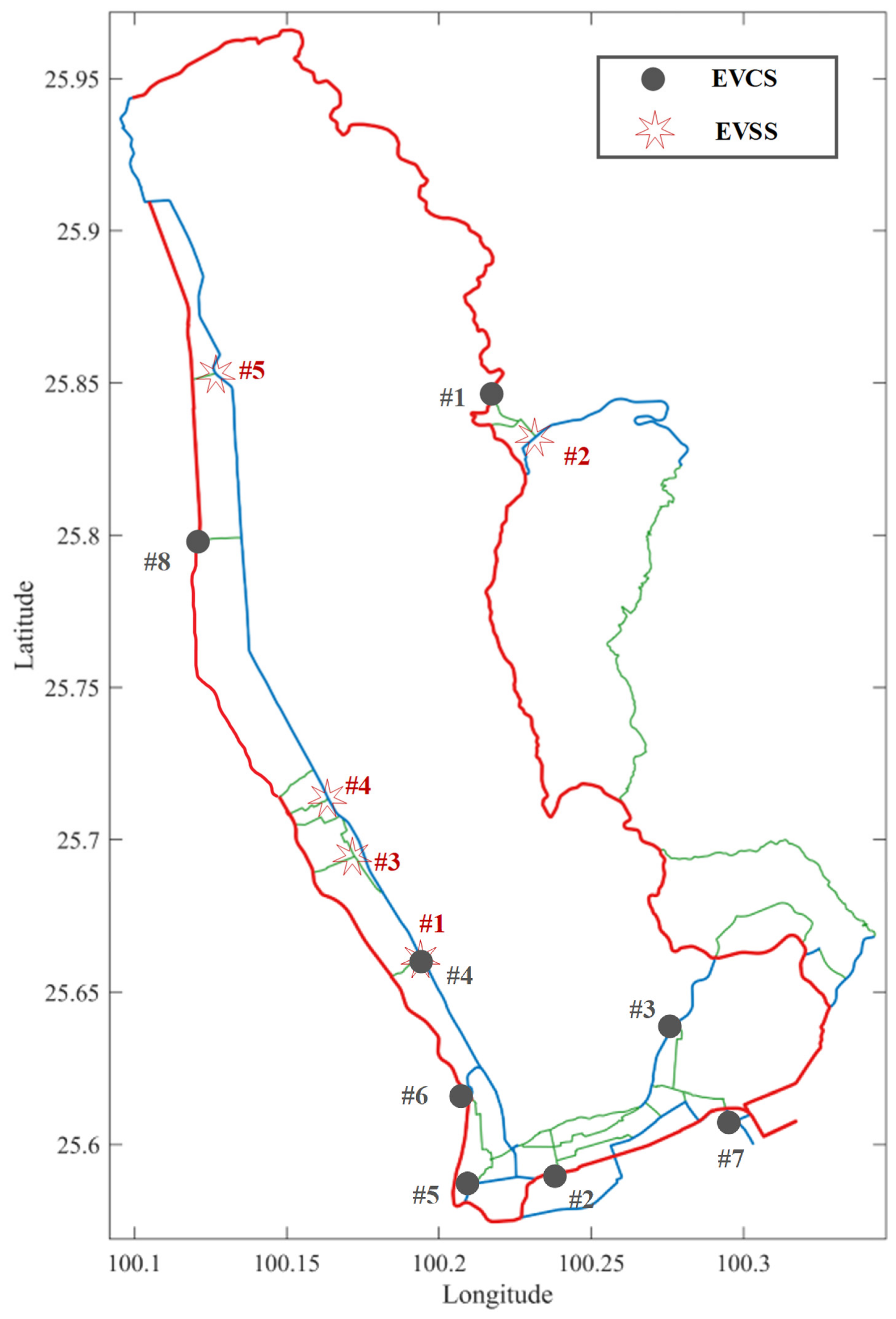
The detailed planning results for EVCS and EVSS obtained from the compromise solution are summarized in

Table 11. Optimal EVCS planning results obtained by RF-SA-NSGA-III.

No.	Traffic Node	Distribution Node	Slow Chargers	Fast Chargers	Rated Power (kW)
1	53	66	17	13	2070
2	11	50	8	15	2040
3	21	41	19	16	2490
4	35	38	6	12	1620
5	2	32	12	12	1800
6	6	29	8	18	2400
7	23	28	8	6	960
8	46	3	8	12	1680

and

Table 12. Optimal EVSS planning results obtained by RF-SA-NSGA-III.

No.	Traffic Node	Distribution Node	Battery Swapping Capacity
1	35	38	9
2	54	36	16
3	37	67	16
4	41	34	15
5	47	33	6

. The proposed scheme determines eight EVCS locations and five EVSS locations in the studied transportation–distribution network, with their spatial distributions illustrated in Figure 9.

The selected EVCSs are distributed among multiple functional areas of the studied road network, including work areas (node 53), commercial areas (nodes 2, 11, and 23), public service areas (nodes 6 and 35), green park areas (node 46), and residential areas (node 21). The deployment results are consistent with the spatial characteristics of charging demand obtained from the demand forecasting analysis. Specifically, work areas and commercial areas exhibit relatively concentrated charging demands during the morning peak period due to commuting and activity accumulation, and EVCSs are accordingly deployed at representative nodes within these regions. Meanwhile, charging stations located in public service, residential, and green park areas provide additional service coverage for vehicles with different travel purposes and temporal demand characteristics.

The planning results also show that EVCS capacities are not uniformly allocated among different locations. Instead, the numbers of slow and fast charging piles, rated power, and daily energy replenishment capacity are jointly optimized according to the corresponding demand characteristics. For example, EVCSs located at nodes 21, 35, and 46 are assigned relatively higher charging capacities, corresponding to their larger daily replenishment demands. This indicates that the proposed method can achieve coordinated optimization of station location and capacity rather than only determining candidate locations.

For EVSS deployment, five battery-swapping stations are selected at nodes 35, 54, 37, 41, and 47, which are mainly distributed in public service areas, work areas, and green park areas. Compared with private EV charging demand, taxi battery-swapping demand presents a stronger relationship with continuous operation requirements and concentrated service periods. Therefore, the obtained EVSS locations are mainly concentrated in areas with intensive transportation activities.

Among the selected locations, node 54 is located in a work area and corresponds to the road-network node with the highest replenishment demand during the system peak period (08:00–08:15) identified in the demand forecasting results. The deployment of an EVSS at this node helps provide timely energy replenishment service for taxis during high-demand periods. In addition, EVSSs located at nodes 35, 37, and 41 in public service areas improve service accessibility by covering additional travel-demand regions, while node 47 in the green park area provides supplementary swapping capacity for surrounding traffic flows. Different swapping capacities are assigned to the selected EVSSs according to their daily replenishment requirements. This differentiated capacity configuration avoids excessive investment at low-demand locations while ensuring sufficient service capability at high-demand areas.

Overall, the obtained EVCS–EVSS planning scheme achieves coordinated deployment of charging and battery-swapping facilities. The selected locations and capacity configurations are jointly optimized according to the spatial distribution of energy replenishment demand and the operational requirements of the coupled transportation–distribution network. In particular, stations with relatively larger capacities are generally allocated to areas with higher energy replenishment demand, while the overall spatial distribution of the planned facilities provides balanced coverage across different functional areas. This consistency between the predicted demand characteristics and the resulting infrastructure deployment provides an additional indication of the rationality and practical feasibility of the proposed planning model.

From an electrical and energy perspective, the obtained results show that the system behavior is closely related to the temporal and spatial distribution of EV replenishment demand and the corresponding EVCS/EVSS capacity allocation. The daily simulation is divided into 96 intervals, and the aggregated replenishment load reaches a peak of 55.13 MW during 08:00–08:15, reflecting the concentration of charging and swapping demand in the morning period. These time-varying demands are mapped to the distribution network through the road–grid coupling relationship and directly affect nodal loading conditions. The power-flow results further indicate that the optimized station configuration maintains the bus voltages within the prescribed operating limits, while the voltage-deviation and network-loss indicators vary with the magnitude and spatial allocation of replenishment demand. Therefore, the final EVCS and EVSS capacities should be interpreted not only as infrastructure sizing decisions, but also as a means of coordinating transportation-side energy demand with distribution-network operating.

5. Conclusions and Future Work

This paper investigates the joint location and capacity optimization problem of EVCSs and EVSSs in a traffic–grid coupled system and proposes a surrogate-assisted evolutionary optimization framework. To address the high computational burden caused by repeated traffic demand evaluation, user service assessment, and multi-period power-flow calculations in conventional evolutionary algorithms, an RF-SA-NSGA-III algorithm is developed. By introducing RF surrogate models to approximate computationally intensive objective evaluations and adopting a periodic real-model correction strategy, the proposed method significantly reduces the dependence on expensive model evaluations. The case study shows that 89.38% of the evaluation calls are performed using surrogate predictions, while the computational time is reduced from 45,706.3 s to 4689.4 s compared with conventional NSGA-III, indicating a substantial improvement in computational efficiency.

A traffic–grid coupled planning scenario is constructed based on an urban transportation network and a distribution system to evaluate the proposed method for EVCS and EVSS joint planning. The repeated-run comparisons and Pareto-based performance indicators show that RF-SA-NSGA-III achieves competitive multi-objective optimization performance under the considered experimental setting while requiring substantially fewer full-model evaluations than conventional NSGA-III. Furthermore, the combination of surrogate prediction and periodic correction helps reduce the influence of surrogate approximation errors while limiting expensive objective evaluations. Overall, the results suggest that the proposed framework provides a favorable balance between computational efficiency and solution quality under the considered case-study conditions.

From a practical planning perspective, the proposed framework can support the coordinated siting and capacity allocation of EVCSs and EVSSs by linking spatiotemporal energy replenishment demand with distribution-network operating requirements. The obtained Pareto solutions provide alternative planning schemes under different priorities, allowing planners to balance investment cost, user service performance, and grid voltage performance. Although the present case study is based on a specific urban transportation network and benchmark distribution system, the overall framework can be extended to other cities or regions by replacing the corresponding transportation topology, EV travel characteristics, spatial demand distribution, distribution-network parameters, and traffic–grid coupling relationships. However, these inputs and coupling parameters must be recalibrated according to local conditions, particularly for highly meshed road networks, heavily constrained distribution systems, or substantially different demand patterns.

The present study adopts a representative daily scenario with 15 min temporal resolution to balance demand representativeness and computational burden. Seasonal temperature information is incorporated through its influence on auxiliary energy consumption and SOC evolution, but independent season-specific scenarios, weekday/weekend travel patterns, nighttime demand characteristics, and other sources of long-term demand variability are not modeled separately. Future work will therefore extend the framework toward multi-scenario planning with more diverse temporal and spatial operating conditions, as well as stochastic travel behavior and dynamic electricity-price information.

Further research will also focus on improving the robustness and validation of the surrogate-assisted optimization framework. In particular, systematic sensitivity analysis of the initial training sample size, surrogate update interval, number of true evaluations per update, and RF settings will be conducted to quantify their influence on prediction accuracy, computational efficiency, and optimization performance. In addition, the repeated-run results indicate that further improvement in run-to-run stability and Pareto-front coverage remains possible. Future studies may therefore investigate more adaptive sample-selection and surrogate-update strategies, together with more detailed operational validation using station utilization, demand-to-capacity ratios, waiting-time statistics, and real-world traffic and charging data.

References

1. Kumar, B.V.; Farhan, A. Multi-Objective Optimization Framework for Strategic Placement of Electric Vehicle Charging Stations and Shunt Capacitors in a Distribution Network Considering Traffic Flow. Appl. Energy 2025, 397, 126284. [Google Scholar] [CrossRef] [Scilit]
2. Ren, H.; Tseng, C.-L.; Wen, F.; Wang, C.; Chen, G.; Li, X. Scenario-Based Optimal Real-Time Charging Strategy of Electric Vehicles with Bayesian Long Short-Term Memory Networks. J. Mod. Power Syst. Clean Energy 2024, 12, 1572–1583. [Google Scholar] [CrossRef] [Scilit]
3. Sawant, V.; Zambare, P. DC Fast Charging Stations for Electric Vehicles: A Review. Energy Convers. Econ. 2024, 5, 54–71. [Google Scholar] [CrossRef] [Scilit]
4. Munusamy, N.; Vairavasundaram, I. Enhancing Grid Stability and V2G Integration by Optimizing Three-Phase Bidirectional EV Chargers Using ANFIS and FPGA-Based Control Systems. Glob. Energy Interconnect. 2025, 8, 1047–1061. [Google Scholar] [CrossRef] [Scilit]
5. Jiang, C.; Lin, Z.; Liu, C.; Chen, F.; Shao, Z. MADDPG-based active distribution network dynamic reconfiguration with renewable energy. Prot. Control Mod. Power Syst. 2024, 9, 143–155. [Google Scholar] [CrossRef] [Scilit]
6. Qiu, C.; Huang, S.; Hu, Y. Review of HVDC Tap. Chin. J. Electr. Eng. 2025, 11, 1–15. [Google Scholar] [CrossRef] [Scilit]
7. Saxena, A.; Shankar, R. An Interactive Operating Demand Response Approach for Hybrid Power Systems Integrating Renewable Energy Sources. Prot. Control Mod. Power Syst. 2024, 9, 174–194. [Google Scholar] [CrossRef] [Scilit]
8. Sarwar, F.A.; Hernando-Gil, I.; Vechiu, I. Review of Energy Management Systems and Optimization Methods for Hydrogen-based Hybrid Building Microgrids. Energy Convers. Econ. 2024, 5, 259–279. [Google Scholar] [CrossRef] [Scilit]
9. Wu, W.; Wang, M.; Tu, L.; Cai, H.; Yan, G.; Qu, X.; Gu, H.; Chen, W. Control, Modeling and Stability Analysis of DRU-Based Grid-Forming Converter. Chin. J. Electr. Eng. 2025, 11, 83–92. [Google Scholar] [CrossRef] [Scilit]
10. Wu, X.; Yang, W.; Zhang, N.; Zhou, C.; Song, J.; Kang, C. A Distributed Computing Algorithm for Electricity Carbon Emission Flow and Carbon Emission Intensity. Prot. Control Mod. Power Syst. 2024, 9, 138–146. [Google Scholar] [CrossRef] [Scilit]
11. Hu, W.; Wang, S.; Du, P. An optimized distribution model for energy system in virtual power plants integrating electric vehicles based on TD3 and DQN. Prot. Control Mod. Power Syst. 2025, 10, 31–48. [Google Scholar] [CrossRef] [Scilit]
12. Mostofa, K.Z.; Fokrul Islam, M.; Islam, M.A.; Basher, M.K.; Abedin, T.; Yap, B.K.; Nur-E-Alam, M. Data-Driven Insights for Optimizing EV Charging Infrastructure: A Case Study on Efficiency and Utilization. Glob. Energy Interconnect. 2025, 8, 997–1009. [Google Scholar] [CrossRef] [Scilit]
13. Qin, W.; Li, X.; Jing, X.; Zhu, Z.; Lu, R.; Han, X. Multi-Temporal Optimization of Virtual Power Plant in Energy-Frequency Regulation Market under Uncertainties. J. Mod. Power Syst. Clean Energy 2024, 13, 675–687. [Google Scholar] [CrossRef] [Scilit]
14. Kumar, B.V.; Farhan, M.A.A. Optimal Simultaneous Allocation of Electric Vehicle Charging Stations and Capacitors in Radial Distribution Network Considering Reliability. J. Mod. Power Syst. Clean Energy 2024, 12, 1584–1595. [Google Scholar] [CrossRef] [Scilit]
15. Xiao, L.; Muttaqi, K.M.; Agalgaonkar, A.P. Reliability assessment of distribution systems under influence of stochastic nature of PV and spatial-temporal distribution of EV load demand. J. Mod. Power Syst. Clean Energy 2025, 13, 1287–1299. [Google Scholar] [CrossRef] [Scilit]
16. Wang, Z.; Zou, J.; Tu, J.; Li, X.; Liu, J.; Wu, H. Towards Sustainable EV Infrastructure: Site Selection and Capacity Pla-nning with Charger Type Differentiation and Queuing-Theoretic Modeling. World Electr. Veh. J. 2025, 16, 600. [Google Scholar] [CrossRef] [Scilit]
17. Zhang, B.; Zhao, M.; Hu, X. Location Planning of Electric Vehicle Charging Station with Users’ Preferences and Waiting Time: Multi-Objective Bi-Level Programming Model and HNSGA-II Algorithm. Int. J. Prod. Res. 2023, 61, 1394–1423. [Google Scholar] [CrossRef] [Scilit]
18. Mehouachi, I.; Trojette, M.; Grayaa, K. Optimal Planning of Electric Vehicle Charging Stations Using a Robust Hybrid Method: A Tunisian Urban Case Study. Transp. Plan. Technol. 2025, 1–27. [Google Scholar] [CrossRef] [Scilit]
19. Su, L.; Xu, Y.; Dong, Z. State-of-health estimation of lithium-ion batteries: A comprehensive literature review from cell to pack levels. Energy Convers. Econ. 2024, 5, 224–242. [Google Scholar] [CrossRef] [Scilit]
20. Wang, H.; Chen, S.; Yuan, J.; Xia, M.; Chen, Z.; Li, G.; Folly, K.A.; Lin, Y.; Ma, Y.; Yang, J. Pricing-based Coordinated Scheduling for Multiple EV Charging Stations Considering Capacity Prediction and Service Radius. Energy Convers. Econ. 2025, 6, 225–236. [Google Scholar] [CrossRef] [Scilit]
21. Zhang, Y.; He, P.; Ren, W.; Jiao, J.; Long, Z.; Jian, Y. A Customer Satisfaction-Based Optimization Model for the Charging and Discharging Path and Battery Swapping Stations’ Site Selection of Electric Vehicles. Front. Energy Res. 2024, 12, 1353268. [Google Scholar] [CrossRef] [Scilit]
22. Lai, Z.; Li, S. Towards a Multimodal Charging Network: Joint Planning of Charging Stations and Battery Swapping Stations for Electrified Ride-Hailing Fleets. Transp. Res. Part B Methodol. 2024, 183, 102928. [Google Scholar] [CrossRef] [Scilit]
23. Qi, W.; Zhang, Y.; Zhang, N. Scaling up Electric-Vehicle Battery Swapping Services in Cities: A Joint Location and Repairable-Inventory Model. Manag. Sci. 2020, 69, 6855–6875. [Google Scholar] [CrossRef] [Scilit]
24. Gull, M.S.; Khalid, M.; Arshad, N. Multi-Objective Optimization of Battery Swapping Station to Power up Mobile and Stationary Loads. Appl. Energy 2024, 374, 124064. [Google Scholar] [CrossRef] [Scilit]
25. Yu, Y.; Jiang, H.; Zhang, N.; Yong, P.; Teng, F.; Zhang, J.; Wang, Y.; Strbac, G. Revisiting capacity value of variable renewable energy generation in power systems with high renewable energy penetration. J. Mod. Power Syst. Clean Energy 2025, 13, 1593–1603. [Google Scholar] [CrossRef] [Scilit]
26. Ji, Z.; Liu, X.; Tang, D. Game-theoretic applications for decision-making behavior on the energy demand side: A systematic review. Prot. Control Mod. Power Syst. 2024, 9, 1–20. [Google Scholar] [CrossRef] [Scilit]
27. Zu, S.; Sun, L. Research on Location Planning of Urban Charging Stations and Battery-Swapping Stations for Electric Vehicles. Energy Rep. 2022, 8, 508–522. [Google Scholar] [CrossRef] [Scilit]
28. EL-Qasery, M.; Abbou, A.; Laamim, M.; Id-Khajine, L.; Rochd, A. Comparative Analysis of GA and PSO Algorithms for Optimal Cost Management in On-Grid Microgrid Energy Systems with PV-Battery Integration. Glob. Energy Interconnect. 2025, 8, 572–580. [Google Scholar] [CrossRef] [Scilit]
29. Jing, Y.; Liang, M.; Wang, H.; Yang, Z.; Li, G.; Márquez, F.P.G.; Yang, J.; Chen, Z. Optimal Economic and Low-carbon Scheduling in Integrated Energy System Considering Multi-level Thermal Energy Coupling and Integrated Demand Response. Energy Convers. Econ. 2025, 6, 83–100. [Google Scholar] [CrossRef] [Scilit]
30. Yang, B.; Zhou, Y.M.; Yan, Y.F.; Su, S.; Li, J.; Yao, W.; Li, H.; Gao, D.; Wang, J. A critical and comprehensive handbook for game theory applications on new power systems: Structure, methodology, and challenges. Prot. Control Mod. Power Syst. 2025, 10, 1–27. [Google Scholar] [CrossRef] [Scilit]
31. Wang, Z.; Pei, Y.; Li, J. Enhancing Non-Dominated Sorting Genetic Algorithm III Using Chaotic Dynamics and Estimated Convergence Point. In Proceedings of the 2025 IEEE International Conference on Systems, Man, and Cybernetics (SMC), Vienna, Austria, 5–8 October 2025; pp. 5540–5545. [Google Scholar] [CrossRef] [Scilit]
32. Zhang, Z.; Ma, S.; Jiang, X. Research on Multi-Objective Multi-Robot Task Allocation by Lin–Kernighan–Helsgaun Guided Evolutionary Algorithms. Mathematics 2022, 10, 4714. [Google Scholar] [CrossRef] [Scilit]
33. Chen, Z.; Dong, Z.Y.; Xu, Y. Anomaly-detection-based learning for real-time data processing in non-intrusive load monitoring. Energy Convers. Econ. 2024, 5, 146–155. [Google Scholar] [CrossRef] [Scilit]
34. Gu, Q.; Wang, Q.; Xiong, N.N.; Jiang, S.; Chen, L. Surrogate-Assisted Evolutionary Algorithm for Expensive Constrained Multi-Objective Discrete Optimization Problems. Complex Intell. Syst. 2022, 8, 2699–2718. [Google Scholar] [CrossRef] [Scilit]
35. Hong, Y.; Liang, S.; Lian, J.; Mai, G.; Zhao, L.; Xu, Y.; Xiang, Y.; Zhang, H.; Liu, F.; Hao, Z. Evolutionary Constrained Optimization Based on Causal Random Forest. Expert Syst. Appl. 2026, 312, 131417. [Google Scholar] [CrossRef] [Scilit]
36. Li, W.; Qiu, Y.; Wang, Z.; Xu, B.; Hao, Z.; Zhang, Q.; Li, Y.; Fan, Z. Surrogate-Assisted Neural Learning and Evolutionary Optimization for Expensive Constrained Multi-Objective Problems. Swarm Evol. Comput. 2025, 97, 102020. [Google Scholar] [CrossRef] [Scilit]
37. Li, J.; Zhan, Z.; Zhang, J. Evolutionary Computation for Expensive Optimization: A Survey. Mach. Intell. Res. 2022, 19, 3–23. [Google Scholar] [CrossRef] [Scilit]
38. Wang, H.; Jin, Y. A Random Forest-Assisted Evolutionary Algorithm for Data-Driven Constrained Multiobjective Combinatorial Optimization of Trauma Systems. IEEE Trans. Cybern. 2018, 50, 536–549. [Google Scholar] [CrossRef] [Scilit] [PubMed]
39. Zhao, F.; Fu, L.; Zhong, M.; Liu, S.; Wang, X.; Huang, J.; Ma, X. Development and Validation of Improved Impedance Functions for Roads with Mixed Traffic Using Taxi GPS Trajectory Data and Simulation. J. Adv. Transp. 2020, 2020, 7523423. [Google Scholar] [CrossRef] [Scilit]
40. He, B.; Yang, B.; Han, Y.; Zhou, Y.; Hu, Y.; Shu, H.; Su, S.; Yang, J.; Huang, Y.; Li, J.; et al. Optimal EVCS Planning via Spatial-Temporal Distribution of Charging Demand Forecasting and Traffic-Grid Coupling. Energy 2024, 313, 133885. [Google Scholar] [CrossRef] [Scilit]
41. Hu, Y.; Yang, B.; He, B.; Li, H.; Gao, D.; Wang, J.; Jiang, L. Optimal Operation and Planning of Hydrogen Refueling Stations for Hydrogen Fuel Cell Vehicles: A Typical Techno-Economic-Environmental Paradigm. Renew. Energy 2026, 256, 124459. [Google Scholar] [CrossRef] [Scilit]
42. Zhou, X.; Liu, X.; Liu, H.; Ji, Z.; Li, F. Optimal Dispatching Strategy for Residential Demand Response Considering Load Participation. Glob. Energy Interconnect. 2024, 7, 38–47. [Google Scholar] [CrossRef] [Scilit]
43. Fiori, C.; Ahn, K.; Rakha, H.A. Power-Based Electric Vehicle Energy Consumption Model: Model Development and Validation. Appl. Energy 2016, 168, 257–268. [Google Scholar] [CrossRef] [Scilit]
44. Chen, S.; Cheng, H.; Lv, S.; Wei, Z.; Li, P.; Jin, J. Learning-Aided Collaborative Optimization of Power, Hydrogen, and Transportation Networks. J. Mod. Power Syst. Clean Energy 2024, 13, 475–487. [Google Scholar] [CrossRef] [Scilit]
45. Liu, G.; Wang, L.; Cui, K.; Guo, P.; Dai, H.; Guo, M.; Xin, L. Assessment of Flexible Interconnection Strategies for the Integration of Electric Vehicles and Renewable Energy in Load-Centric Distribution Networks. Glob. Energy Interconnect. 2025, 8, 447–459. [Google Scholar] [CrossRef] [Scilit]
46. Li, J.; Yang, B.; Huang, J.; Guo, Z.; Wang, J.; Zhang, R.; Hu, Y.; Shu, H.; Chen, Y.; Yan, Y. Optimal Planning of Electricity–Hydrogen Hybrid Energy Storage System Considering Demand Response in Active Distribution Network. Energy 2023, 273, 127142. [Google Scholar] [CrossRef] [Scilit]
Figure 1. Framework of the charging and swapping demand forecasting process.
Algorithms 19 00783 g001
Figure 2. Flowchart of the proposed RF-SA-NSGA-III algorithm.
Algorithms 19 00783 g002
Figure 3. Road network topology and node classification diagram.
Algorithms 19 00783 g003
Figure 4. Schematic diagram of electric-traffic coupling network.
Algorithms 19 00783 g004
Figure 5. Energy replenishment demand characteristics under different classifications. (a) Daily energy replenishment power profiles of different EV categories. (b) Charging energy demand profiles of different functional areas.
Algorithms 19 00783 g005
Figure 6. Spatiotemporal distribution of EV energy replenishment demand across road network nodes.
Algorithms 19 00783 g006
Figure 7. Voltage fluctuation profiles of the optimal solutions obtained by different algorithms.
Algorithms 19 00783 g007
Figure 8. Three-dimensional Pareto-optimal solution set obtained by RF-SA-NSGA-III.
Algorithms 19 00783 g008
Figure 9. Spatial distribution of optimal EVCS and EVSS locations obtained by RF-SA-NSGA-III.
Algorithms 19 00783 g009