Quasi-Random Sampling-Enhanced Metaheuristic Algorithms for CAMD-Based Solvent Selection in Octacosanol Extraction

Abstract

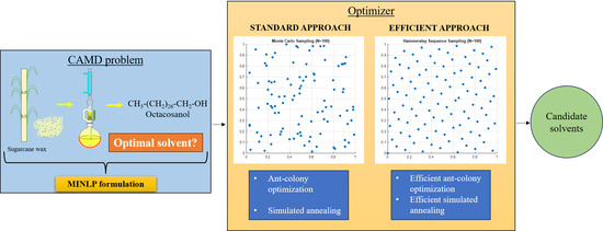
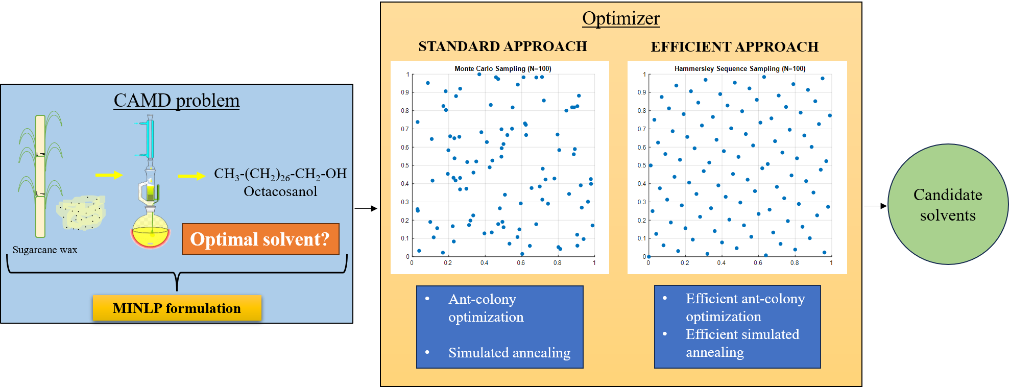
This study develops a computer-aided molecular design (CAMD) framework for selecting solvents to extract octacosanol from multicomponent sugarcane wax. The solvent-selection problem is formulated as a mixed-integer nonlinear programming problem in which candidate solvents are assembled from UNIFAC functional groups and evaluated using the net distribution coefficient and net solvent selectivity. Four metaheuristic solvers—ant-colony optimization (ACO), simulated annealing (SA), efficient ant-colony optimization (EACO), and efficient simulated annealing (ESA)—are compared in terms of solvent quality and computational efficiency. EACO and ESA replace selected pseudo-random samples with Hammersley sequence samples to improve multidimensional sampling uniformity. All four solvers identify the same highest-ranked candidate, while ACO and EACO require substantially fewer objective-function evaluations than SA and ESA. The SA-based methods provide greater diversity among lower-ranked candidates. Relative to their conventional counterparts, EACO reduces the computational cost by 14.2% and ESA by 16% while preserving the leading solvent candidates. Overall, the CAMD framework consistently identifies promising candidates, including ethane and propanal, for octacosanol extraction, and quasi-random sampling improves the efficiency of both metaheuristic approaches.

1. Introduction

Natural products often occur as complex mixtures, making the isolation of target compounds an important objective because of their specific applications. In industry, extraction is one of the most widely used separation operations, and solvent selection is critical to its effectiveness. In an extraction system, the solvent should selectively attract the desired compound into the extract phase while leaving impurities in the raffinate phase. For a given system, solvents are generally selected using one of three approaches [1,2]:

(a)

Experimental screening of candidate solvents for the system.

(b)

Database screening based on physical, chemical, and related properties.

(c)

Computer-aided molecular design (CAMD) to generate optimal solvents.

The first two approaches may not identify the best solvent and can lead to incomplete evaluation. Although experimental screening provides reliable results, it is often expensive and time-consuming. In contrast, CAMD uses thermodynamic models to design solvents tailored to target performance requirements [1]. In CAMD, molecules are generated by combining available functional groups to ensure that the resulting structures meet desired performance metrics. Because the number of possible group combinations and attachment patterns is extremely large, combinatorial optimization is central to this problem.

Papadimitriou and Steiglitz [3] define a combinatorial optimization problem as one that seeks an optimal solution, such as an integer, permutation, or graph structure, from a finite or countably infinite set. Common examples include the travelling salesman and scheduling problems [4]. CAMD can also be formulated as a combinatorial optimization problem. Metaheuristic algorithms, including ant colony optimization (ACO), evolutionary computation, genetic algorithms, and simulated annealing (SA), use random number generation during the search process and their performance strongly depends on the quality of the sampling. In this work, we enhance SA and ACO by replacing the pseudo-random numbers used in conventional implementations with quasi-Monte Carlo samples generated through Hammersley sequence sampling (HSS). The resulting algorithms, efficient ant-colony optimization (EACO) and efficient simulated annealing (ESA), preserve k-dimensional sampling uniformity.

Although ESA and EACO have been applied separately in previous studies, their performance has not been compared systematically with that of conventional SA and ACO for the same molecular-design problem. It therefore remains unclear whether HSS provides consistent benefits across distinct metaheuristic search mechanisms or whether its effectiveness depends on the application. This study addresses that gap by comparing all four algorithms for a nutraceutical-extraction problem: selecting solvents to recover octacosanol from multicomponent sugarcane wax.

Nutraceuticals are health-promoting compounds derived from food sources, including plant and animal waxes and apple and grape seeds, that provide benefits beyond basic nutrition [5]. Because sugarcane is produced worldwide at large scale, recovering nutraceuticals from sugarcane residues is an important separation opportunity [6]. Sugarcane wax contains long-chain alcohols, esters, aldehydes, acids, and saturated hydrocarbons. Among its saturated alcohols, policosanols contain 18–34 carbon atoms and a hydroxyl group (-OH) on the alpha carbon. Octacosanol, a 28-carbon policosanol, is particularly promising because of its reported immune-supporting, anti-Parkinsonian, and anti-fatigue effects [7,8]. Accordingly, this study uses CAMD to identify optimal solvents for extracting octacosanol from the multicomponent mixture in sugarcane wax.

The remainder of this paper is organized as follows. Section 2 reviews octacosanol extraction, CAMD, molecular construction, the UNIFAC group-contribution method, and the solvent-selection formulation. Section 3 presents ACO, SA, HSS, EACO, and ESA, together with their algorithmic frameworks, parameter values, and the mapping of continuous samples to discrete molecular-design variables. Section 4 compares the solvents identified by the four solvers and evaluates the computational efficiency of EACO and ESA relative to ACO and SA. The final section summarizes the best solvent candidates and the comparative performance of the four algorithms.

2. The Solvent Selection Problem

Policosanols offer several health benefits, including lipid regulation, anti-atherosclerotic effects, and support in managing obesity, etc. [8,9]. Among them, octacosanol is a particularly promising nutraceutical. Numerous studies have attempted to extract policosanols or octacosanol-rich fractions from sugarcane using methods such as Soxhlet extraction, supercritical CO₂ (99.99%), and subcritical dimethyl ether extraction [10,11,12,13]. However, in most cases, solvent selection has been ad hoc, guided largely by prior experience. Further, the experimental studies observed that the obtained extracts still contain some amounts of impurities. Such an approach risks overlooking solvents with superior performance, especially because experimentally screening a large solvent set is costly and time-consuming. A systematic, performance-based solvent selection strategy is therefore essential.

Solvent choice in extraction depends on properties such as the distribution coefficient, selectivity, recoverability, and environmental safety [1,5]. In this study, we focus on distribution coefficient and solvent selectivity.

• Distribution coefficient is the ratio of the desired solute’s concentration in the solvent phase to its concentration in the original mixture.
• Solvent selectivity measures how effectively a solvent attracts the desired solute relative to undesired components.

These metrics form the basis of the solvent selection optimization problem developed in the following sections.

2.1. Computer-Aided Molecular Design

The group contribution method estimates molecular properties—melting and boiling points, density, viscosity, and activity coefficients (γ)—from the functional groups that make up a molecule. As distribution coefficient and selectivity can be determined using activity coefficients, this method is central to our analysis.

CAMD reverses this logic: Instead of predicting properties from a molecule, it constructs molecules from available groups to optimize performance metrics [1]. CAMD has been widely applied in designing solvents for separation processes, refrigerants, polymers, pharmaceuticals, and more [1,2,14,15,16,17]. Recent advances even integrate machine learning to generate molecules with drug-like characteristics [18].

In CAMD, molecules are built by selecting the following:

• $N_1$, representing the total number of functional groups.
• $N_2^{\left(i\right)}$, representing the index of each group (i = 1, …, N₁).

Feasible molecular structures must satisfy chemical bonding rules—the octet rule for covalent systems [5]. Thus, $N_1$ and $N_2^{\left(i\right)}$ serve as decision variables, while bonding constraints ensure chemically valid structures.

Figure 1 outlines the CAMD workflow for identifying optimal solvents for sugarcane wax extraction. The process begins by identifying mixture components and estimating their activity coefficients, followed by formulating and solving the solvent-performance optimization problem.

2.2. Group Contribution Method: UNIFAC

The group contribution method (GCM) predicts thermodynamic properties by decomposing molecules into functional groups and summing their contributions [19]. This approach is especially valuable when experimental data are unavailable, enabling property estimation across chemical engineering, molecular design, and process simulation.

Among the many properties GCM can predict, activity coefficients are particularly important for mixture behavior. They quantify deviations from ideality, with γ = 1 representing ideal solutions. For solvent design, the most widely used GCM for estimating activity coefficients is UNIFAC, which provides reliable predictions for non-ideal liquid mixtures. For molecule i present in a solution, its activity coefficient, ${\gamma }_i$, is defined as shown in Equation (1) [19].

$$U\left({\gamma }_i\right)=ln {\gamma }_i-\left(ln {\gamma }_i^C + ln {\gamma }_i^R\right)=0$$

(1)

Equation (1) is the standard UNIFAC expression for estimating the activity coefficient. The estimate comprises two contributions: A combinatorial term and a residual term. The combinatorial term accounts for differences in molecular size and shape, whereas the residual term accounts for energetic interactions among the functional groups of the molecules in solution.

Firstly, the combinatorial part is estimated as shown in Equation (2a–f) [19].

$$ln {\gamma }_i^C=\ln \left({\displaystyle \frac{{\Phi }_i}{x_i^b}}\right)+5q_i\ln \left({\displaystyle \frac{{\theta }_i}{{\Phi }_i}}\right)+l_i-{\displaystyle \frac{{\Phi }_i}{x_i^b}}\sum _j{x}_j^b{l}_j$$

(2a)

where

$${\Phi }_i={\displaystyle \frac{r_i{x}_i^b}{{\displaystyle {\sum }_j^{N_C}}{r}_j{x}_j^b}}$$

(2b)

$${\theta }_i={\displaystyle \frac{q_i{x}_i^b}{{\displaystyle {\sum }_j^{N_C}}{q}_j{x}_j^b}}$$

(2c)

$$l_i=5\left(r_i-q_i\right)-\left(r_i-1\right)$$

(2d)

where ${\Phi }_i$ and ${\theta }_i$ are the molecular volume fraction and the molecular surface area fraction, respectively, of molecule i, ranging from 1 to N_C molecules. This is followed by the estimation of van der Waals’ volume, $r_i$, and surface area, $q_i$, using Equation (2e) and Equation (2f), respectively.

$$r_i=\sum _g^{N_g}{\nu }_g^{\left(i\right)}{R}_g$$

(2e)

$$q_i=\sum _g^{N_g}{\nu }_g^{\left(i\right)}{Q}_g$$

(2f)

where $R_g$ and $Q_g$ are van der Waals’ group volume and group surface area values ranging from the $i$ to the $N_g$ groups and where ${\nu }_g^{\left(i\right)}$ is the total number of functional groups present in the molecule. The values of $R_g$ and $Q_g$ are obtained from the literature for this study while the estimation of the residual part is based on Equation (3a–e) [19].

$$ln {\gamma }_i^R=\sum _k{v}_k^i\left(\ln {\Gamma }_k-\ln {\Gamma }_k^i\right)$$

(3a)

where ${\Gamma }_k$ is defined as the residual activity coefficient of group k in a solution, shown in Equation (3b). Similarly, ${\Gamma }_k^i$ is defined as the residual activity coefficient of group k in a solution containing only molecules of type i.

$$n{\Gamma }_k=Q_k\left[1-ln\left(\sum _m{\Theta }_m{\Psi }_{mk}\right)-\sum _m{\displaystyle \frac{{\Theta }_m{\Psi }_{km}}{\sum _n{\Theta }_n{\Psi }_{nm}}}\right]$$

(3b)

where m and n represent all of the functional groups in the molecule, ${\Theta }_m$ is the surface fraction of group m in Equation (3c), which is further expressed in terms of mole fraction of groups present in the bulk phase, Equation (3d), and where, lastly, the temperature-dependent parameter as per UNIFAC is ${\Psi }_{mn}$, in Equation (3e) [19].

$${\Theta }_m={\displaystyle \frac{Q_m{X}_m}{\sum _m{Q}_m{X}_m}}$$

(3c)

$$X_m={\displaystyle \frac{{\sum }_i^j{\nu }_m^{\left(i\right)}{x}_j}{{\sum }_1^j{\sum }_1^n{\nu }_m^{\left(i\right)}{x}_j}}$$

(3d)

$${\Psi }_{mn}=e^{-{\displaystyle \frac{a_{mn}}{T}}}$$

(3e)

In Equation (3e), $a_{mn}$ is called the group interaction parameter (represents interaction of group m with group n). This is defined as the difference in the energy level between group m and group n or between two of the main groups of m. In the latter case, the interaction parameter is zero because of the same energy levels of both the groups. These values are obtained from the literature for every group [19].

In the next subsection, we discuss the development of the optimization problem for solvent selection used in this study along with the parameters important to build the optimization problem.

2.3. Solvent Selection Optimization Problem

This section formulates the solvent-selection optimization problem for extracting a desired compound from a multicomponent mixture. Solvent performance is evaluated using the distribution coefficient ($m$) and solvent selectivity ($\beta$), both estimated using the UNIFAC group contribution method. For a binary mixture containing desired solute B, undesired solute A, and solvent S, these quantities are defined by Equation (4a) and Equation (4b), respectively [5].

$$m_B={\displaystyle \frac{C_{B, S}}{C_{B, A}}}={\displaystyle \frac{{\gamma }_{BA}}{{\gamma }_{BS}}}$$

(4a)

$${\beta }_B={\displaystyle \frac{m_B}{m_A}}={\displaystyle \frac{C_{B,S}}{C_{A,S}}}={\displaystyle \frac{{\gamma }_{SA}}{{\gamma }_{BS}}}$$

(4b)

Here, C_x,y denotes the concentration of component x in phase y. Because the present system contains multiple undesired solutes, the binary definitions of the distribution coefficient and solvent selectivity are extended by weighting each undesired solute A_i, i = 1, 2, …, N, by its mole fraction. Equation (5a) and Equation (5b) define the resulting net distribution coefficient and net solvent selectivity, respectively, following the formulation reported in the literature [5].

$$m_{net}={\displaystyle \frac{{\gamma }_{BX}}{{\gamma }_{BS}}}$$

(5a)

$${\beta }_{net}=\sum _{i=1}^N{x}_{A_i}{\beta }_i$$

(5b)

where ${\gamma }_{BX}={\displaystyle \frac{{\sum }_{i=1}^N{x}_{A_i}{\gamma }_{B{A}_i}}{{\sum }_{i=1}^N{x}_{A_i}}}$ and ${\beta }_i$ is the solvent selectivity value obtained between desired solute B and the undesired solute A_i. The system of undesired solutes is represented as X. That is the reason the activity coefficient (${\gamma }_{BX}$) is defined between the desired solute B and every undesired solute A_i by weighing against their corresponding mole fraction.

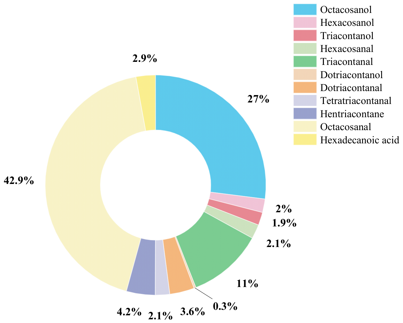
Next, in this study, the multicomponent system is built based on earlier experimental studies. Sugarcane wax is a complex matrix of compounds. Therefore, we considered a few of the most abundant compounds reported in the literature to be present in this multicomponent mixture, while the desired solute remains octacosanol [13]. Figure 2 shows the system of compounds considered in this study along with their corresponding mole fractions as reported in the literature.

Solvent generation requires a defined set of UNIFAC groups. In this study, candidate molecules are constructed by selecting up to 12 groups from the 20 groups listed in

Table 1. Various UNIFAC groups ranging from general hydrocarbons to aromatic (groups starting with “A”), and a few other functional groups such as hydroxyl, carboxylic acid, aldehyde, and ketone.

$\mathit{i}$	${\mathit{N}}_2^{\left(\mathit{i}\right)}$	$\mathit{i}$	${\mathit{N}}_2^{\left(\mathit{i}\right)}$	$\mathit{i}$	${\mathit{N}}_2^{\left(\mathit{i}\right)}$	$\mathit{i}$	${\mathit{N}}_2^{\left(\mathit{i}\right)}$	$\mathit{i}$	${\mathit{N}}_2^{\left(\mathit{i}\right)}$
1	CH3–	2	CH2<	3	–CH<	4	>C<	5	H2O
6	CH2=CH–	7	–CH=CH–	8	–CH=C<	9	CH2=C<	10	–OH
11	ACH	12	AC	13	ACCH3	14	ACCH2	15	ACCH
16	ACOH	17	CH3–CO–	18	–CH2–CO–	19	–CHO	20	–COOH

, which were obtained from Fredenslund et al. [19]. Each group is indexed from 1 to 20. A molecule may contain multiple instances of the same group, but the final structure must satisfy the octet rule. This feasibility constraint is expressed mathematically in Equation (6) [2].

$${\displaystyle \sum _i^{N_1}}{b}_i=2(N_1-1)$$

(6)

where $b_i$ determines the number of groups that can be attached to the group index i.

Lastly, another molecular constraint, the boiling point of CAMD solvent, is included in the formulation based on the definition proposed by Joback’s true boiling point as shown in Equation (7) [20]. In order to have a broad computational search range, the true boiling point of a generated solvent is set to vary from −100 °C to 400 °C.

$$TBP (°\mathrm{C})=198.15+{\displaystyle \sum _{i=1}^{N_1}}{T}^{BP}\left(N_2^{\left(i\right)}\right)$$

(7)

Finally, our objective is to maximize the net distribution coefficient of the solvent generated by any of the 20 groups listed in Table 1, so that it can isolate octacosanol with a net solvent selectivity (${\beta }_{net,min}$) greater than or equal to the set value from the ten undesired solutes present in the mixture. Based on these, the optimization problem is defined as shown in Equation (8).

$$\begin{array}{c}\hfill \underset{N_1,N_2^{\left(i\right)}}{max}{ m}_{net}\hfill \\ \mathrm{s}.\mathrm{t}.\hfill \\ \hfill {\beta }_{net}\ge {\beta }_{net,min}\hfill \\ \hfill U\left({\gamma }_i\right)=0\hfill \\ \hfill {\displaystyle \sum _i^{N_1}}{b}_i=2(N_1-1)\hfill \\ \hfill 2 \le N_1\le 12\hfill \\ \hfill 1\le N_2^{\left(i\right)}\le 20, \forall i \mathsf{ϵ} [1,2,\dots ,N_1]\hfill \\ \hfill -100\le TBP (°\mathrm{C})\le 400\hfill \end{array}$$

(8)

Equation (8) shows that the decision variables, $N_1$ and $N_2^{\left(i\right)}$, are discrete and that the objective function and constraints, which are evaluated using UNIFAC, are nonlinear; therefore, the problem is a mixed-integer nonlinear programming problem. The combinatorial complexity arises because the groups in Table 1 can be connected in many feasible ways. To address this challenge, metaheuristic algorithms such as ACO and SA, and their efficient variants ESA and EACO, are used to identify optimal solvent candidates. The next section presents the four solvers used in this work to solve this optimization problem.

3. Algorithmic Framework

This section presents the four metaheuristic algorithms used to solve the solvent-selection problem. It first reviews conventional ACO and SA, then introduces Hammersley sequence sampling and explains how it is incorporated into ACO and SA to form EACO and ESA, respectively. The section also specifies the algorithmic frameworks, parameter values, and efficiency measures used for the comparative analysis.

3.1. Ant-Colony Optimization

Ant-colony optimization (ACO) is a nature-inspired metaheuristic based on the foraging behavior of ants, introduced by Dorigo to solve combinatorial optimization problems [21]. In nature, ants deposit pheromones as they return from food sources, allowing other ants to follow promising paths. Because shorter paths are traversed more frequently, pheromone accumulates faster on them, gradually guiding the colony toward the shortest route [21,22]. Similarly, in ACO, artificial ants construct solutions using pheromone information and, when available, heuristic information. At iteration iter, the probability of selecting solution component j from state I, (${\mathbb{P}}_{ij}^{iter}$) is given by Equation (9) [21,22].

$${\mathbb{P}}_{ij}^{iter}={\displaystyle \frac{{\tau }_{ij}^{\alpha }\left(iter\right){\eta }_{ij}^{\beta }}{{\sum }_{iter}{\tau }_{ij}^{\alpha }\left(iter\right){\eta }_{ij}^{\beta }}}$$

(9)

where ${\tau }_{ij}^{\alpha }$ and ${\eta }_{ij}^{\beta }$ are the pheromone value and edge desirability for edge ij, respectively, at iteration iter, while $\alpha$ and $\beta$ determine the influence of pheromone and heuristic information [22]. After all ants construct solutions, pheromone trails are updated according to solution quality, with additional pheromone assigned to edges in better solutions, as shown in Equation (10) [22].

$${\tau }_{ij}\left(iter+1\right)=\rho {\tau }_{ij}\left(iter\right)+∆{\tau }_{ij}\left(iter\right)$$

(10)

where $\rho$ is the pheromone evaporation factor and $∆{\tau }_{ij}$ is the pheromone addition for edge ij.

The artificial pheromone along the path acts as a communication bridge among artificial ants. In the less favourable solution routes, the artificial pheromone decays gradually, whereas in the better solution routes, the pheromone concentration increases, as observed in Equation (9). Eventually, iterative updating of pheromone values based on information gained from earlier iterations encourages the artificial ants towards the optimal solution in the solution space.

The solution construction in this study is based on an incremental manner, i.e., an ant first probabilistically chooses one of the solutions from the archive based on Equation (11) [22].

$${\mathbb{P}}_i={\displaystyle \frac{{\omega }_i}{{\displaystyle {\sum }_{j=1}^K}{\omega }_j}}$$

(11)

where ${\omega }_i$ is the weight associated with solution i, i is the rank of the solution in the archive, and K is the size of the solution archive. The weight is defined as shown in Equation (12) [22].

$${\omega }_i={\displaystyle \frac{\mathrm{e}\mathrm{x}\mathrm{p}(-\frac{{\left(i-1\right)}^2}{2{\left(qK\right)}^2})}{qK\sqrt{2\pi }}}$$

(12)

where q is the algorithmic parameter of ACO and the mean of the Gaussian function is 1. However, in this study, the optimization problem is a mixed integer non-linear programming problem. Therefore, using a set of probability density functions, a multimodal one-dimensional density function is obtained. To estimate the multimodal density function, the following equation, Equation (13), is used [23].

$$G_j\left(x\right)={\displaystyle \sum _{i=1}^K}{\omega }_i{\displaystyle \frac{\exp \left(-\frac{{\left(x-{\mu }_i\right)}^2}{2{\sigma }_i^2}\right)}{{\sigma }_i\sqrt{2\pi }}}, i,j\in \left\{1,\dots ,K\right\}$$

(13)

where $G_j\left(x\right)$ is the Gaussian kernel, ${\omega }_i$ is the weight associated with individual Gaussian function, and ${\mu }_i$ and ${\sigma }_i$ are the vector means of the individual solution components and standard deviations, respectively.

3.2. Simulated Annealing

Simulated annealing (SA) is a probabilistic metaheuristic for finding near-optimal solutions to optimization problems. It is inspired by metallurgical annealing, in which a material is heated and then slowly cooled so that its particles settle into a low-energy state. Similarly, SA gradually reduces a control parameter, analogous to temperature, to guide the search toward lower objective-function values while allowing occasional uphill moves. If cooling is sufficiently slow, the system can approach thermal equilibrium at each temperature level, described by the Boltzmann distribution. At temperature T, the probability of occupying energy level E_i is given by Equation (14) [24].

$${\mathbb{P}}_T={\displaystyle \frac{exp\left(-\frac{E_i}{k_{B}T}\right)}{Z}}$$

(14)

where 1/Z is the normalization factor and k_B is Boltzmann’s constant (1.3806 × 10⁻²³ J/K).

In SA, the objective function represents the system energy. Starting from an initial configuration, the algorithm generates a candidate configuration by perturbing the current one. If the candidate has a lower objective value, the move is accepted. If it has a higher objective value, the move may still be accepted with probability according to the Metropolis criterion, given in Equation (15) [24,25].

$$\mathrm{Accept} \mathrm{the} \mathrm{move} \mathrm{if} {Pr}_{accept}\le A_{ij}=\left\{\begin{array}{c}exp\left(-{\displaystyle \frac{∆E}{T}}\right) if \Delta E=E_j-E_i\ge 0\\ 1 otherwise\end{array}\right\} \forall i,j\in \mathrm{move}$$

(15)

where $A_{ij}$ is the probability of accepting a transition from state i to state j. At high temperatures, SA accepts more uphill moves, improving exploration of the solution space. As temperature decreases, the probability of accepting such moves declines, allowing the algorithm to converge while reducing the risk of becoming trapped in local optima.

ACO and SA differ substantially in their search mechanisms. SA follows a single-solution trajectory, exploring the search space through successive perturbations of one candidate solution; therefore, complex problems may require many iterations, and escape from local optima depends on the Metropolis criterion [24,26]. In contrast, ACO uses multiple ants to construct solutions in parallel and share information through pheromone trails, which improves exploration and reduces the likelihood of premature trapping [21]. However, as a population-based heuristic, ACO may still miss some high-quality regions of the search space.

3.3. Hammersley Sequence Sampling

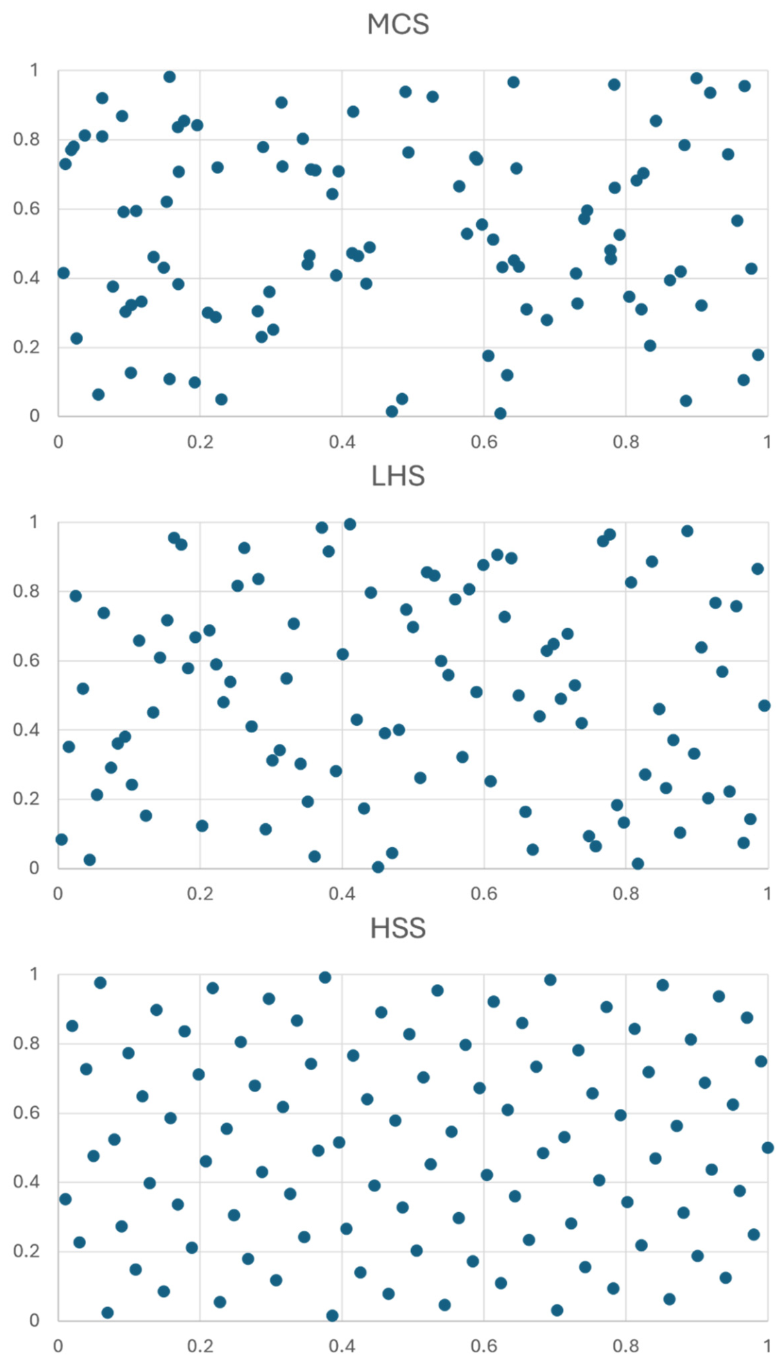
Sampling strongly affects optimization efficiency. Monte Carlo sampling uses independently generated pseudo-random numbers over the sampling domain; these samples are statistically unbiased and useful for estimating probabilities and objective-function values in complex systems [25]. However, pseudo-random samples can cluster in some regions while leaving others unexplored, as shown in Figure 3 for two random variables. This reduces sampling efficiency and often requires many samples to adequately cover the search space [25,27]. Quasi-random methods, such as Hammersley sequence sampling (HSS), reduce this clustering by distributing samples more uniformly. HSS, developed by Kalagnanam and Diwekar based on Hammersley points [28], provides better multidimensional uniformity than Monte Carlo methods and other methods, such as Latin hypercube sampling, as illustrated in Figure 3 [25].

In both metaheuristics, ACO and SA, HSS is introduced to improve the distribution of samples within the solution space, thereby enhancing exploration to build higher-quality solutions and reducing the computational cost. The following subsections discuss more about the implementation of HSS in these algorithms.

3.4. Efficient Ant-Colony Optimization (EACO)

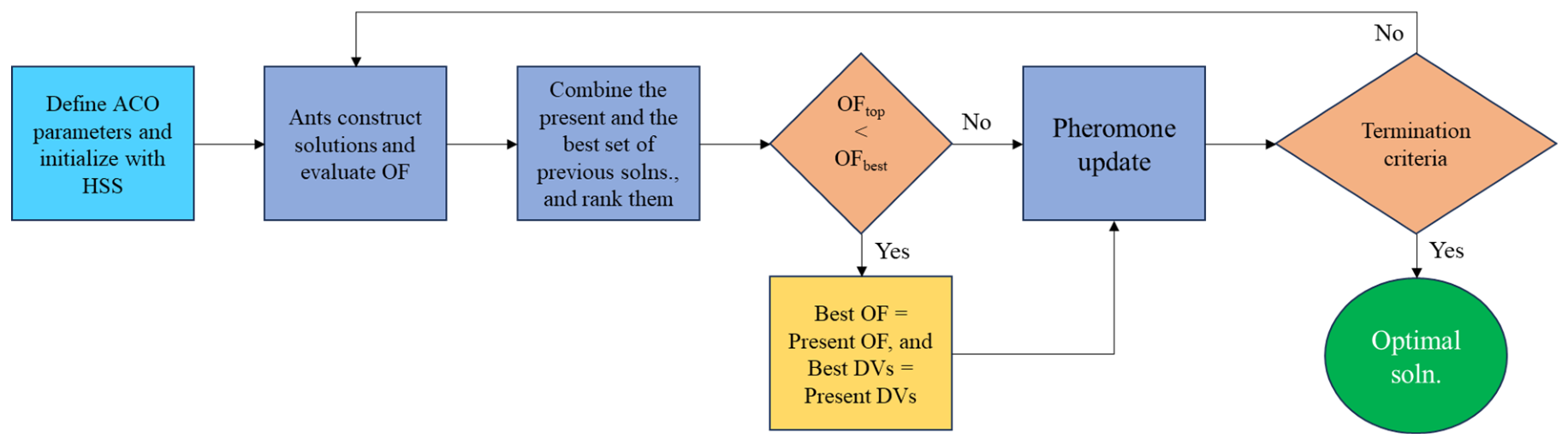
ACO can suffer from premature convergence when excessive pheromone accumulation reduces population diversity and limits exploration. Several variants have been developed to improve its performance, including the elitist ant system, rank-based ant system, max–min ant system, ant colony system, hypercube-based ACO, and hybrids with local search methods such as tabu search [4]. Efficient ant-colony optimization (EACO) improves ACO by replacing selected pseudo-random numbers with quasi-random numbers generated using Hammersley sequence sampling (HSS) [22,27]. Reported studies show that EACO improves computational efficiency by 3–71% for selected problems [22]. In this study, HSS is used only during initialization, where k-dimensional uniformity is most important for generating the initial ant population, as shown in Figure 4.

Both ACO and EACO use 30 artificial ants, a pheromone decay factor of 0.75, and a solution archive of size 1500 × 13. The first 12 columns store the functional-group indices that define each candidate solvent, and the final column stores its objective-function value. The algorithms terminate when the absolute difference between successive objective-function values is below 10⁻⁶ or when 20,000 iterations have been completed. These parameter values were adopted from a previous study in which multiple combinations were evaluated [27]. Because solvent generation is subject to several constraints, the objective is implemented as a penalty function using the extended oracle penalty method [29]. The method transforms the objective into an equality constraint of the form OF − Ω, where the oracle value Ω is set to 3, and penalizes candidate solvents that violate the constraints in Equation (8) with cumulative residual res(x). Equation (16a,b) define the penalty function used in this study; further details are provided by Schlüter and Gerdts [29].

$$p\left(x\right)=\left\{\begin{array}{c}-\left|f\left(x\right)-\Omega \right|, if f\left(x\right)\le \Omega , and res\left(x\right)\le {10}^{-6}\\ \alpha \left|f\left(x\right)-\Omega \right|+\left(1-\alpha \right)res\left(x\right), if f\left(x\right)>\Omega or res\left(x\right)>{10}^{-6} \end{array}\right.$$

(16a)

where $\alpha$ is given by:

$$\alpha =\left\{\begin{array}{c}\begin{array}{c}{\displaystyle \frac{\left|f\left(x\right)-\Omega \right|\left(\frac{6\sqrt{3}-2}{6\sqrt{3}}\right)-res\left(x\right)}{\left|f\left(x\right)-\Omega \right|-res\left(x\right)}}, if f\left(x\right)>\Omega and res\left(x\right)<{\displaystyle \frac{\left|f\left(x\right)-\Omega \right|}{3}} \\ 1-{\displaystyle \frac{1}{2\sqrt{\frac{\left|f\left(x\right)-\Omega \right|}{res\left(x\right)}}}}, if f\left(x\right)>\Omega and {\displaystyle \frac{\left|f\left(x\right)-\Omega \right|}{3}}\le res\left(x\right)\le \left|f\left(x\right)-\Omega \right|\\ {\displaystyle \frac{1}{2}}\sqrt{{\displaystyle \frac{\left|f\left(x\right)-\Omega \right|}{res\left(x\right)}}}, if f\left(x\right)>\Omega and res\left(x\right)>\left|f\left(x\right)-\Omega \right|\end{array}\\ 0, if f\left(x\right)\le \Omega \end{array}\right.$$

(16b)

3.5. Efficient Simulated Annealing (ESA)

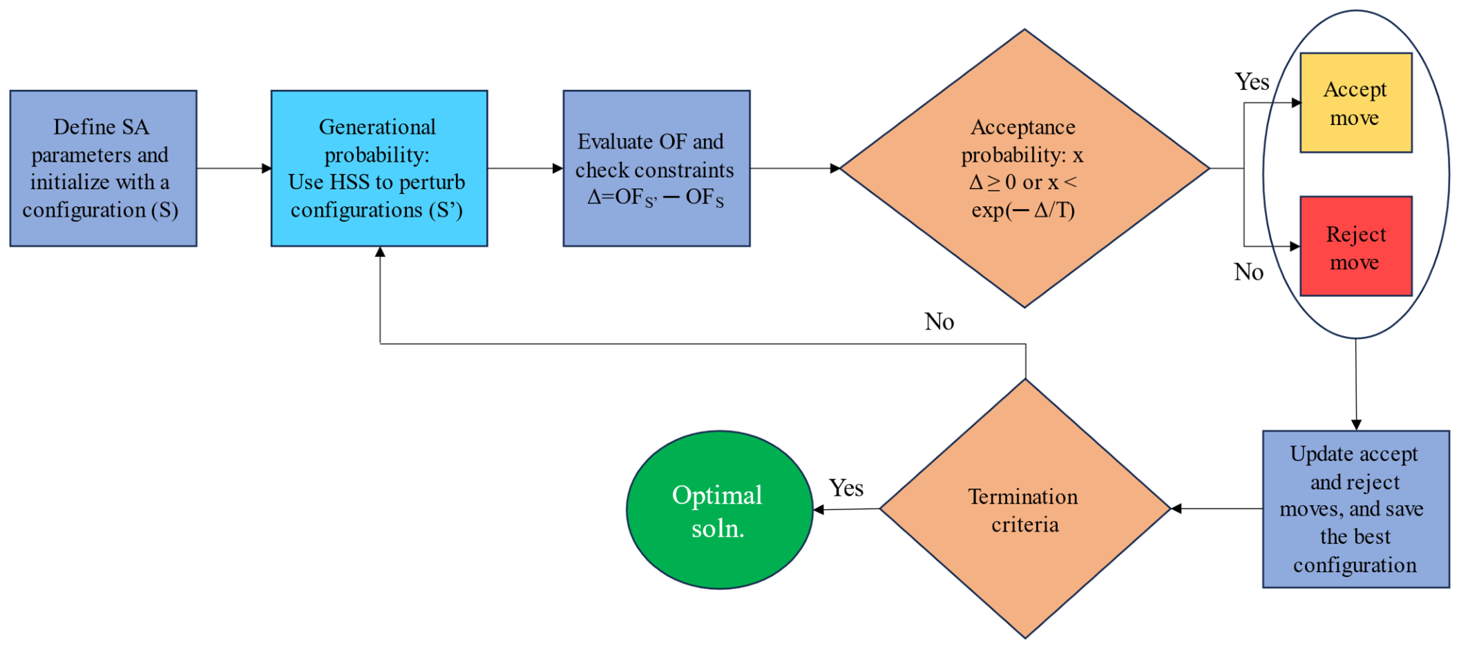
SA uses two probabilities: the acceptance probability, $A_{ij}$, and the generational probability, $G_{ij}$ [25]. The acceptance probability determines whether a candidate configuration is accepted, whereas the generational probability controls how new configurations are sampled near the current solution. SA efficiency depends strongly on the generational probability [25]. In conventional SA, these probabilities are generated using uniformly distributed pseudo-random numbers, which can cluster sampled moves and require longer Markov chains. Several SA variants, including fast SA and hybrid SA, modify the generational probability or cooling schedule, or combine SA with methods such as differential evolution and genetic algorithms [30,31,32]. However, these approaches do not directly address sampling uniformity. Kim and Diwekar improved configurational sampling by incorporating HSS into SA, leading to efficient simulated annealing (ESA) [25]. As shown in Figure 5, ESA replaces pseudo-random numbers with HSS to generate configuration moves, thereby improving k-dimensional uniformity and reducing the Markov chain length required at each temperature level. Studies report that ESA is approximately 30–54% more efficient than conventional SA in terms of total moves [25].

In this study, the initial SA temperature is 50 and is reduced by a cooling factor of 0.85 until it reaches the freezing temperature of 10⁻⁷. SA uses pseudo-random numbers for all four generational probabilities and the acceptance probability. In ESA, the four generational probabilities are generated using HSS, while the acceptance probability remains pseudo-random. Both algorithms terminate when the temperature falls below the freezing temperature or when the candidate solvent remains unchanged for 10 consecutive moves across different samples. The algorithmic parameters have been rigorously used in various previous studies and, therefore, the same values have been used in the study [1,2,5].

3.6. Mapping of Continuous Samples to Discrete Samples

The optimization problem considered here is a mixed-integer nonlinear programming problem, whereas both pseudo-random sampling and HSS generate coordinates in a continuous domain. These coordinates must therefore be mapped to the discrete decision variables that specify the number and identities of the functional groups. In SA and ESA, each sampling dimension is partitioned into equal subintervals, and the subinterval containing a generated coordinate determines the corresponding integer value. In ACO and EACO, each continuous coordinate is mapped to a predefined set of allowable molecular-design values; the midpoint between consecutive allowable values defines the assignment boundary, and coordinates outside the prescribed range are assigned to the nearest bound. The resulting discrete decision variables are then used to construct the molecular structure and evaluate the objective function and constraints.

4. Results and Discussions

This study evaluates the efficiency of ACO, SA, EACO, and ESA for solving the CAMD problem of selecting solvents to extract octacosanol from a multicomponent sugarcane wax mixture. In Equation (8), the minimum net solvent selectivity, βnet,min, is set to 1.2. Each algorithm is then used to generate the top 20 candidate solvents.

4.1. Candidate Solvents Using ACO and SA

Based on the algorithm parameters mentioned in the methodology section, the candidate solvents generated using ACO and SA are listed in

Table 2. List of candidate solvents generated using ACO.

Sno.	UNIFAC Groups in the Candidate Solvent	${\mathbf{m}}_{\mathbf{n}\mathbf{e}\mathbf{t}}$	${\mathsf{\beta }}_{\mathbf{n}\mathbf{e}\mathbf{t}}$
1	2 CH3	529.49	1.69
2	1 CH3, 1 CHO	168.32	7.29
3	1 CH3, 1 CH2, 1 CHO	64.58	5.41
4	2 CH3, 1 CH, 1 CHO	30.89	4.34
5	1 CH3, 2 CH2, 1 CHO	30.71	4.34
6	2 CH3, 1 CH2, 1 CH, 1 CHO	17.43	3.65
7	1 CH3, 3 CH2, 1 CHO	17.36	3.65
8	3 CH3, 1 C, 1 CHO	15.71	3.67
9	3 CH3, 1 CH2, 1 C, 1 CHO	10.35	3.20
10	2 CH3, 1 CH=C, 1 CHO	4.03	3.17
11	2 CH3, 1 CH, 1 COOH	3.408	3.11
12	1 CH3, 2 CH2, 1 COOH	3.401	3.11
13	1 CH3, 1 CH2, 1 COOH	3.07	4.29
14	2 CH3, 1 CH2, 1 CH, 1 COOH	3.03	2.43
15	1 CH3, 3 CH2, 1 COOH	3.03	2.43
16	3 CH3, 1 C, 1 COOH	2.84	2.42
17	2 CH3, 2 CH2, 1 CH, 1 COOH	2.57	2.03
18	3 CH3, 1 CH2, 3 CH, 1 CHO, 1 COOH	2.45	3.54
19	1 CH3, 3 CH2, 1 CH, 1 CHO, 1 COOH	2.23	4.38
20	4 CH3, 1 CH2, 2 CH, 1 CH=C, 2 CHO	1.48	2.97

and

Table 3. List of candidate solvents generated using SA.

Sno.	UNIFAC Groups in the Candidate Solvent	${\mathbf{m}}_{\mathbf{n}\mathbf{e}\mathbf{t}}$	${\mathsf{\beta }}_{\mathbf{n}\mathbf{e}\mathbf{t}}$
1	2 CH3	529.49	1.69
2	1 CH3, 1 CHO	168.32	7.29
3	1 CH3, 1 CH2, 1 CHO	64.58	5.41
4	2 CH3, 1 CH, 1 CHO	30.89	4.34
5	1 CH3, 2 CH2, 1 CHO	30.71	4.34
6	2 CH3, 1 CH2, 1 CH, 1 CHO	17.43	3.65
7	1 CH3, 3 CH2, 1 CHO	17.36	3.65
8	3 CH3, 1 C, 1 CHO	15.71	3.67
9	3 CH3, 2 CH, 1 CHO	11.19	3.18
10	2 CH3, 2 CH2, 1 CH, 1 CHO	11.15	3.18
11	1 CH3, 4 CH2, 1 CHO	11.12	3.18
12	3 CH3, 1 CH2, 1 C, 1 CHO	10.35	3.20
13	3 CH3, 1 CH2, 2 CH, 1 CHO	7.84	2.83
14	2 CH3, 3 CH2, 1 CH, 1 CHO	7.82	2.83
15	1 CH3, 5 CH2, 1 CHO	7.80	2.83
16	2 CH3, 1 CH=C, 1 CHO	4.03	3.17
17	2 CH3, 1 CH2, 1 CH=C, 1 CHO	3.73	2.81
18	2 CH3, 1 CH, 1 COOH	3.408	3.11
19	1 CH3, 2 CH2, 1 COOH	3.401	3.11
20	1 CH3, 1 CH2, 1 COOH	3.07	4.29

, respectively.

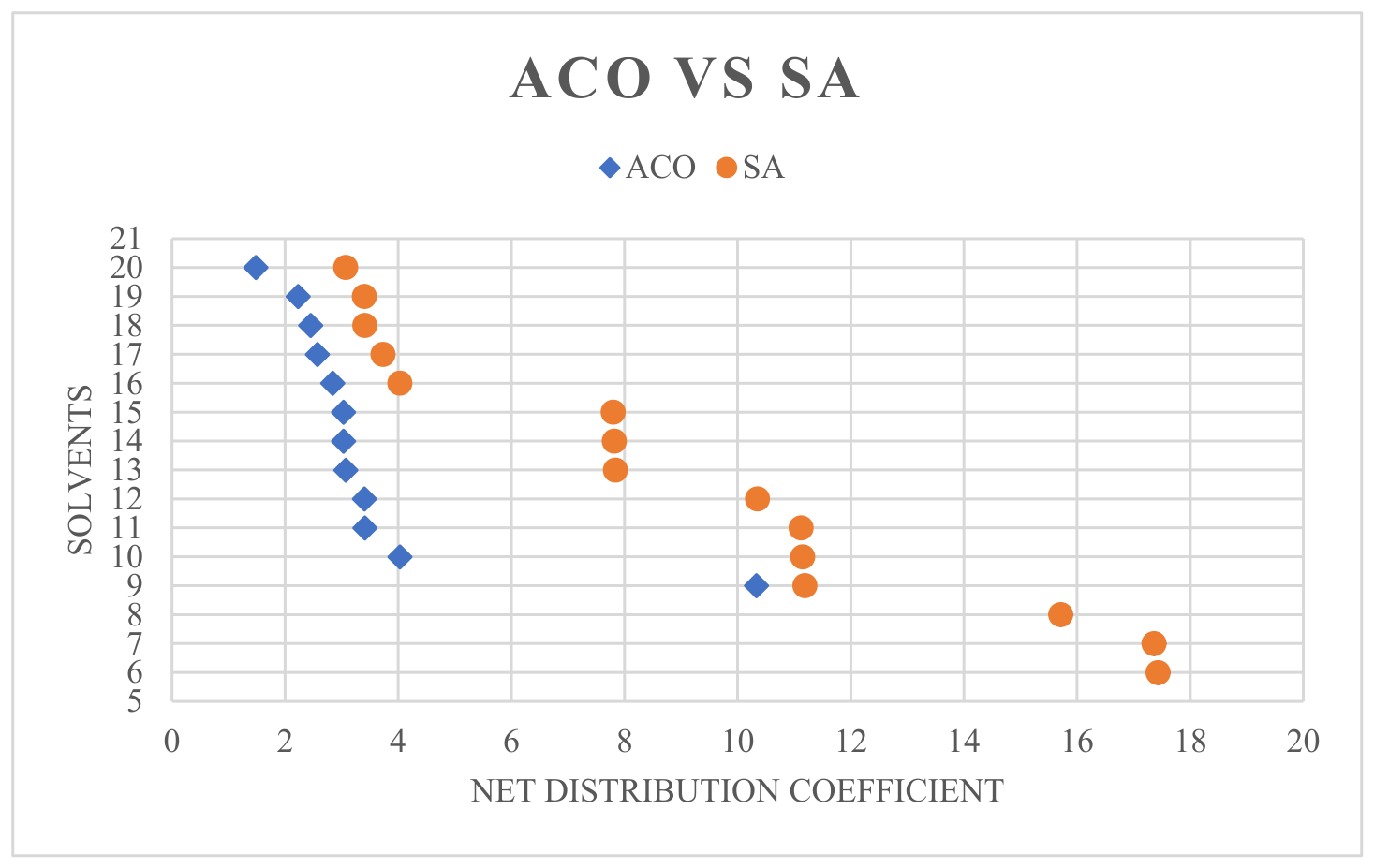
As shown in Table 2 and Table 3 and Figure 6, ACO and SA identify the same top nine candidate solvents. SA yields stronger candidates among the remaining 11 positions but requires 1,271,876 objective-function evaluations, compared with 153,330 for ACO. Thus, ACO uses only 12.05% of the computational effort required by SA. This difference arises because SA produces one solution per run and must be restarted from different initial values to obtain multiple candidates, whereas ACO generates all 20 candidates in a single run.

4.2. Candidate Solvents Using EACO and ESA

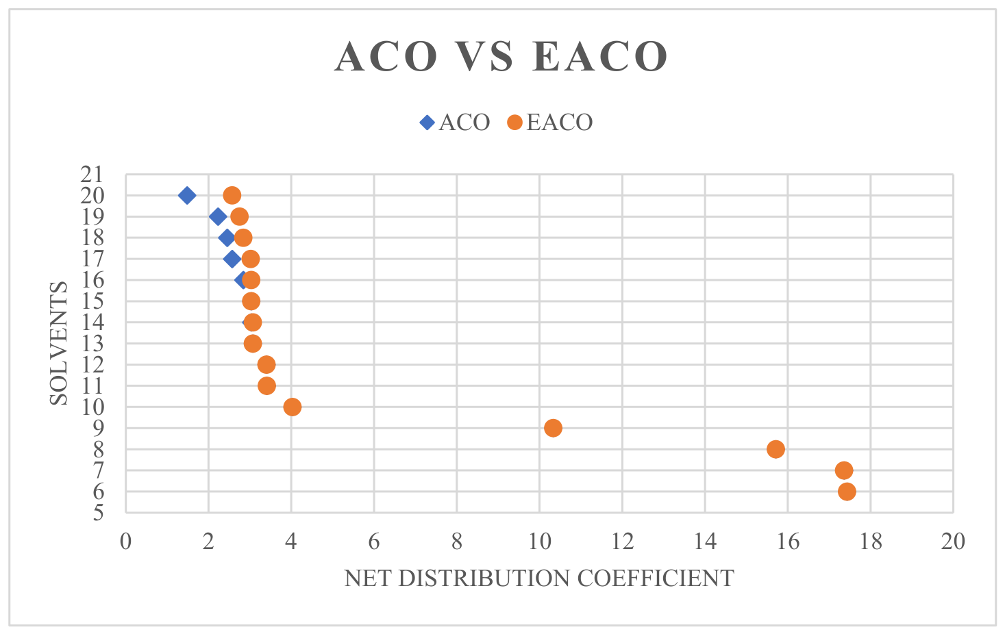
The same optimization problem was then solved using EACO and ESA.

Table 4. List of candidate solvents generated using EACO.

Sno.	UNIFAC Groups in the Candidate Solvent	${\mathbf{m}}_{\mathbf{n}\mathbf{e}\mathbf{t}}$	${\mathsf{\beta }}_{\mathbf{n}\mathbf{e}\mathbf{t}}$
1	2 CH3	529.49	1.69
2	1 CH3, 1 CHO	168.32	7.29
3	1 CH3, 1 CH2, 1 CHO	64.58	5.41
4	2 CH3, 1 CH, 1 CHO	30.89	4.34
5	1 CH3, 2 CH2, 1 CHO	30.71	4.34
6	2 CH3, 1 CH2, 1 CH, 1 CHO	17.43	3.65
7	1 CH3, 3 CH2, 1 CHO	17.36	3.65
8	3 CH3, 1 C, 1 CHO	15.71	3.67
9	3 CH3, 1 CH2, 1 C, 1 CHO	10.35	3.20
10	2 CH3, 1 CH=C, 1 CHO	4.03	3.17
11	2 CH3, 1 CH, 1 COOH	3.408	3.11
12	1 CH3, 2 CH2, 1 COOH	3.401	3.11
13	2 CH3, 2 CH2, 2 CH, 2 CHO	3.07	3.78
14	1 CH3, 1 CH2, 1 COOH	3.07	4.29
15	2 CH3, 1 CH2, 1 CH, 1 COOH	3.03	2.43
16	1 CH3, 3 CH2, 1 COOH	3.03	2.43
17	2 CH3, 1 CH2, 2 CH, 2 CHO	3.02	4.08
18	3 CH3, 1 C, 1 COOH	2.84	2.42
19	2 CH3, 1 CH2, 1 C, 2 CHO	2.75	4.51
20	3 CH3, 2 CH, 1 COOH	2.57	2.03

lists the candidate solvents obtained from EACO for the problem defined in Equation (8). As shown in Figure 7, EACO and conventional ACO identify the same top 15 solvents, while EACO yields stronger candidates among the remaining five positions. EACO requires 131,550 objective-function evaluations, a 14.20% reduction relative to ACO.

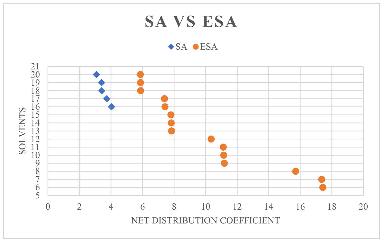
Similarly,

Table 5. List of candidate solvents generated using ESA.

Sno.	UNIFAC Groups in the Candidate Solvent	${\mathbf{m}}_{\mathbf{n}\mathbf{e}\mathbf{t}}$	${\mathsf{\beta }}_{\mathbf{n}\mathbf{e}\mathbf{t}}$
1	2 CH3	529.49	1.69
2	1 CH3, 1 CHO	168.32	7.29
3	1 CH3, 1 CH2, 1 CHO	64.58	5.41
4	2 CH3, 1 CH, 1 CHO	30.89	4.34
5	1 CH3, 2 CH2, 1 CHO	30.71	4.34
6	2 CH3, 1 CH2, 1 CH, 1 CHO	17.43	3.65
7	1 CH3, 3 CH2, 1 CHO	17.36	3.65
8	3 CH3, 1 C, 1 CHO	15.71	3.67
9	3 CH3, 2 CH, 1 CHO	11.19	3.18
10	2 CH3, 2 CH2, 1 CH, 1 CHO	11.15	3.18
11	1 CH3, 4 CH2, 1 CHO	11.12	3.18
12	3 CH3, 1 CH2, 1 C, 1 CHO	10.35	3.20
13	3 CH3, 1 CH2, 2 CH, 1 CHO	7.84	2.83
14	2 CH3, 3 CH2, 1 CH, 1 CHO	7.82	2.83
15	1 CH3, 5 CH2, 1 CHO	7.80	2.83
16	4 CH3, 2 CH2, 1 C, 1 CHO	7.42	2.85
17	3 CH3, 2 CH2, 1 C, 1 CHO	7.39	2.85
18	4 CH3, 3 CH, 1 CHO	5.88	2.57
19	3 CH3, 2 CH2, 2 CH, 1 CHO	5.87	2.57
20	2 CH3, 4 CH2, 1 CH, 1 CHO	5.86	2.57

lists the optimal solvents obtained by solving the solvent-selection optimization problem with ESA. Similar to Figure 7, Figure 8 compares the net distribution coefficient values for the solvents generated by SA and ESA, excluding the top five candidates. ESA again outperformed SA by identifying five better solvents among the lower-ranked 20 candidates. ESA required 1,068,448 objective function evaluations, which is 16% fewer than SA.

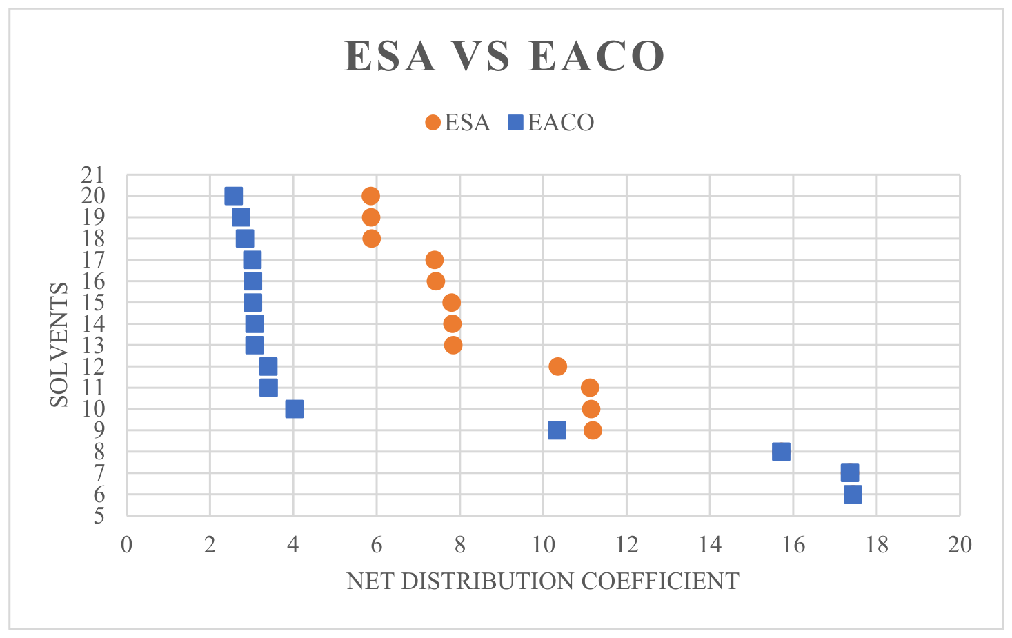
Figure 9 presents solvents obtained by ESA and EACO. This figure shows the same trend as the comparison of SA and ACO in Figure 6. The top 9 solvents found using EACO are the same as those found in the ESA case, while the bottom 11 are better solvents found by ESA as compared with those found with EACO. However, EACO consumes 12.3% of the computational cost when compared with ESA.

4.3. Comparison of All Four Algorithms

Taken together, the results show that all four algorithms are reliable for identifying the highest-quality region of the solvent-design space. ACO, SA, EACO, and ESA return the same leading candidate, represented by two CH₃ groups, with a net distribution coefficient of 529.49 and a net solvent selectivity of 1.69. They also reproduce the same next several high-ranked candidates, indicating that the dominant solvent structures are robust to both the underlying search mechanism and the choice of pseudo-random or Hammersley sequence sampling.

The principal distinction is computational effort. ACO requires 153,330 objective-function evaluations, compared with 1,271,876 for SA, because its population-based search generates multiple candidates in a single run, whereas SA follows a single-solution trajectory and requires repeated runs to assemble a ranked set. Incorporating Hammersley sequence sampling further reduces the effort: EACO requires 131,550 evaluations, 14.20% fewer than ACO, and ESA requires 1,068,448 evaluations, approximately 16% fewer than SA. Thus, EACO is the most computationally efficient method among the four, while ESA improves substantially on conventional SA but remains more expensive than either ant-colony method.

The algorithms also differ in the diversity of lower-ranked solutions. SA and ESA explore a broader range of candidate structures beyond the common leading set, while ACO and EACO converge more rapidly on a compact group of high-performing candidates. Hammersley sequence sampling improves both algorithm families without changing the best solutions: EACO preserves the top 15 ACO candidates and strengthens several lower-ranked positions, whereas ESA identifies five stronger lower-ranked candidates than SA. Accordingly, EACO is preferable when the primary objective is rapid identification of the best solvents, while SA or ESA may be useful when greater structural diversity is desired. Overall, the quasi-random variants provide the best balance within their respective algorithm families by preserving solution quality while reducing objective-function evaluations.

Sensitivity analysis has also been conducted for all four solvers to check whether the candidate solvents depend on the selected algorithmic parameters. The cooling factor in SA and ESA was increased from 0.85 to 0.9, while in ACO and EACO, the pheromone decay was increased to 0.85 from 0.75. In each case, the modified parameter yielded the same candidate solvents as the reference configuration. This consistency in the results obtained using both conventional and enhanced algorithms shows that the optimum solution is robust to the selected algorithmic parameter. Consequently, both SA and ACO frameworks show confidence in the reliability and reproducibility of solvent design.

Finally, solving the proposed optimization problem using the four solvers resulted in the same top candidate solvents. In addition, EACO and ESA obtained a better list of candidate solvents when compared with their counterparts’ solutions, which indicates that the advantages of Hammersley sequence sampling have been utilized. Further, we have also experimentally validated the ability to extract octacosanol from an industrially obtained sugarcane wax using two solvents, propanal and 2-methylpropanal, which aligned with those of the CAMD results.

5. Conclusions

This study developed and evaluated a CAMD-based framework for designing solvents to extract octacosanol from multicomponent sugarcane wax. The solvent-selection problem was formulated as a mixed-integer nonlinear programming problem using UNIFAC-based estimates of the net distribution coefficient and net solvent selectivity. Four metaheuristic solvers—ACO, SA, EACO, and ESA—were compared to assess both solvent quality and computational efficiency. Across all methods, the highest-ranked candidates were consistent, indicating that the CAMD formulation reliably identifies strong solvent structures for the target extraction. Chemically, the best candidate solvent, ethane, achieved the highest net distribution coefficient, and other solvents, aldehyde- and carboxylic-acid-containing structures, also satisfied the selectivity constraint and appeared among the top candidates. Incorporating the Hammersley sequence sampling in ACO and SA has improved the search performance of EACO and ESA by distributing samples more uniformly across the solution space. EACO reduced the number of objective function evaluations by 14.2% compared with ACO while retaining the same top-ranked solvents and improving some lower-ranked candidates. ESA also identified better lower-ranked candidates than SA and reduced the computational cost by almost 16%. Overall, ACO- and EACO-based approaches were substantially more computationally efficient than SA-based approaches for generating a list of candidate solvents, whereas SA and ESA provided improved diversity among lower-ranked solutions. Furthermore, the candidate solvents remained the same in all four cases when sensitivity analysis was performed. These results show that quasi-random sampling can enhance metaheuristic solvent design and that the proposed CAMD framework is robust for complex nutraceutical extraction problems.

References

1. Kim, K.-J.; Diwekar, U.M.; Joback, K.G. Greener solvent selection under uncertainty. In ACS Symposium Series; American Chemical Society: Washington, DC, USA, 2002; Volume 819, pp. 224–237. [Google Scholar]
2. Kim, K.J.; Diwekar, U.M. Efficient combinatorial optimization under uncertainty. 2. Application to stochastic solvent selection. Ind. Eng. Chem. Res. 2002, 41, 1285–1296. [Google Scholar] [CrossRef] [Scilit]
3. Papadimitriou, C.; Steiglitz, K. Combinatorial Optimization: Algorithms and Complexity; Dover Publications, Inc.: New York, NY, USA, 1982; Available online: https://api.semanticscholar.org/CorpusID:265900001 (accessed on 10 August 2026).
4. Blum, C. Ant colony optimization: Introduction and recent trends. Phys. Life Rev. 2005, 2, 353–373. [Google Scholar] [CrossRef] [Scilit]
5. Nistala, V.S.; Bhartiya, S.; Juvekar, V.; Diwekar, U.M. Designing Solvents to Extract Nutraceuticals from Multicomponent Sugar Cane Wax Using a Computer-Aided Molecular Design (CAMD) Approach. Ind. Eng. Chem. Res. 2026, 65, 11655–11670. [Google Scholar] [CrossRef] [Scilit]
6. Food and Agriculture Organization of the United Nations. Food and Agriculture Organization of the United Nations (2025)—with major processing by Our World in Data. “Sugar cane production—UN FAO” 2026. Available online: https://archive.ourworldindata.org/20260727-131016/grapher/sugar-cane-production.html (accessed on 10 August 2026).
7. Sharma, R.; Matsuzaka, T.; Kaushik, M.K.; Sugasawa, T.; Ohno, H.; Wang, Y.; Motomura, K.; Shimura, T.; Okajima, Y.; Mizunoe, Y.; et al. Octacosanol and policosanol prevent high-fat diet-induced obesity and metabolic disorders by activating brown adipose tissue and improving liver metabolism. Sci. Rep. 2019, 9, 5169. [Google Scholar] [CrossRef] [Scilit] [PubMed]
8. Shen, J.; Luo, F.; Lin, Q. Policosanol: Extraction and biological functions. J. Funct. Foods 2019, 57, 351–360. [Google Scholar] [CrossRef] [Scilit]
9. Marinangeli, C.P.F.; Jones, P.J.H.; Kassis, A.N.; Eskin, M.N.A. Policosanols as nutraceuticals: Fact or fiction. Crit. Rev. Food Sci. Nutr. 2010, 50, 259–267. [Google Scholar] [CrossRef] [Scilit] [PubMed]
10. Asikin, Y.; Takahashi, M.; Hirose, N.; Hou, D.X.; Takara, K.; Wada, K. Wax, policosanol, and long-chain aldehydes of different sugarcane (Saccharum officinarum L.) cultivars. Eur. J. Lipid Sci. Technol. 2012, 114, 583–591. [Google Scholar] [CrossRef] [Scilit]
11. Kamchonemenukool, S.; Ho, C.T.; Boonnoun, P.; Li, S.; Pan, M.H.; Klangpetch, W.; Weerawatanakorn, M. High Levels of Policosanols and Phytosterols from Sugar Mill Waste by Subcritical Liquefied Dimethyl Ether. Foods 2022, 11, 2937. [Google Scholar] [CrossRef] [Scilit] [PubMed]
12. Irmak, S.; Dunford, N.T.; Milligan, J. Policosanol contents of beeswax, sugar cane and wheat extracts. Food Chem. 2006, 95, 312–318. [Google Scholar] [CrossRef] [Scilit]
13. Attard, T.M.; McElroy, C.R.; Rezende, C.A.; Polikarpov, I.; Clark, J.H.; Hunt, A.J. Sugarcane waste as a valuable source of lipophilic molecules. Ind. Crops Prod. 2015, 76, 95–103. [Google Scholar] [CrossRef] [Scilit]
14. Cignitti, S.; Rodriguez-Donis, I.; Abildskov, J.; You, X.; Shcherbakova, N.; Gerbaud, V. CAMD for entrainer screening of extractive distillation process based on new thermodynamic criteria. Chem. Eng. Res. Des. 2019, 147, 721–733. [Google Scholar] [CrossRef] [Scilit]
15. Salazar, J.; Diwekar, U.; Joback, K.; Berger, A.H.; Bhown, A.S. Solvent selection for post-combustion CO2 capture. Energy Procedia 2013, 37, 257–264. [Google Scholar] [CrossRef] [Scilit]
16. Trevizo, C.; Daniel, D.; Nirmalakhandan, N. Screening alternative degreasing solvents using multivariate analysis. Environ. Sci. Technol. 2000, 34, 2587–2595. [Google Scholar] [CrossRef] [Scilit]
17. Kim, K.J.; Diwekar, U.M. Integrated solvent selection and recycling for continuous processes. Ind. Eng. Chem. Res. 2002, 41, 4479–4488. [Google Scholar] [CrossRef] [Scilit]
18. Button, A.; Merk, D.; Hiss, J.A.; Schneider, G. Automated de novo molecular design by hybrid machine intelligence and rule-driven chemical synthesis. Nat. Mach. Intell. 2019, 1, 307–315. [Google Scholar] [CrossRef] [Scilit]
19. Fredenslund, A.; Gmehling, J.; Rasmussen, P. Vapor-Liquid Equilibria Using UNIFAC: A Group Contribution Method, 1st ed.; Elsevier Scientific Pub. Co.: Amsterdam, The Netherlands, 1977. [Google Scholar]
20. Joback, K.G.; Reid, R.C. Estimation of pure-component properties from group contributions. Chem. Eng. Commun. 1987, 57, 233–243. [Google Scholar] [CrossRef] [Scilit]
21. Dorigo, M.; Stu¨tzle, T. Ant Colony Optimization; The MIT Press: Cambridge, MA, USA, 2004. [Google Scholar]
22. Diwekar, U.; Gebreslassie, B. Efficient ant colony optimization (EACO) algorithm for deterministic optimization. Int. J. Swarm Intell. Evol. Comput. 2016, 5, 131. [Google Scholar]
23. Socha, K.; Dorigo, M. Ant colony optimization for continuous domains. Eur. J. Oper. Res. 2008, 185, 1155–1173. [Google Scholar] [CrossRef] [Scilit]
24. Aarts, E.; Korst, J. Simulated Annealing and Boltzmann Machines: A Stochastic Approach to Combinatorial Optimization and Neural Computing; John Wiley & Sons Ltd.: Essex, UK, 1989. [Google Scholar]
25. Kim, K.J.; Diwekar, U.M. Hammersley stochastic annealing: Efficiency improvement for combinatorial optimization under uncertainty. IIE Trans. 2002, 34, 761–777. [Google Scholar] [CrossRef] [Scilit]
26. van Laarhoven, P.; Aarts, E. Simulated Annealing: Theory and Applications; Springer-Science+ Business Media, B.V.: Berlin/Heidelberg, Germany, 1992. [Google Scholar]
27. Gebreslassie, B.H.; Diwekar, U.M. Efficient ant colony optimization for computer aided molecular design: Case study solvent selection problem. Comput Chem. Eng. 2015, 78, 1–9. [Google Scholar] [CrossRef] [Scilit]
28. Kalagnanam, J.R.; Diwekar, U.M. An efficient sampling technique for off-line quality control. Technometrics 1997, 39, 308–319. [Google Scholar] [CrossRef]
29. Schlüter, M.; Gerdts, M. The oracle penalty method. J. Glob. Optim. 2010, 47, 293–325. [Google Scholar] [CrossRef] [Scilit]
30. Szu, H.; Hartley, R. Fast simulated annealing. Phys. Lett. A 1987, 122, 157–162. [Google Scholar] [CrossRef] [Scilit]
31. Azizi, N.; Zolfaghari, S.; Liang, M. Hybrid simulated annealing with memory: An evolution-based diversification approach. Int. J. Prod. Res. 2010, 48, 5455–5480. [Google Scholar] [CrossRef] [Scilit]
32. Yu, X.; Liu, Z.; Wu, X.; Wang, X. A hybrid differential evolution and simulated annealing algorithm for global optimization. J. Intell. Fuzzy Syst. 2021, 41, 1375–1391. [Google Scholar] [CrossRef] [Scilit]
Figure 1. Schematic flowchart of solvent generation using CAMD.
Algorithms 19 00678 g001
Figure 2. Multicomponent system present in sugarcane wax and their mole fractions.
Algorithms 19 00678 g002
Figure 3. 100 sample points ranging from 0 to 1 generated using Monte Carlo, LHS and HSS showing the k-dimensional uniformity property.
Algorithms 19 00678 g003
Figure 4. The working mechanism of the ACO algorithm with HSS initialization. Note: OF: objective function, DV: decision variable.
Algorithms 19 00678 g004
Figure 5. The working mechanism of the SA algorithm with HSS initialization.
Algorithms 19 00678 g005
Figure 6. Comparison of net distribution coefficient values of solvents generated using SA and ACO, except the top five.
Algorithms 19 00678 g006
Figure 7. Comparison of net distribution coefficient values of solvents generated using ACO and EACO, except the top five.
Algorithms 19 00678 g007
Figure 8. Comparison of net distribution coefficient values of solvents generated using SA and ESA, except the top five.
Algorithms 19 00678 g008
Figure 9. Comparison of the net distribution coefficient values of solvents generated using ESA and EACO, except the top five.
Algorithms 19 00678 g009