Imperfect Debugging SRGM with FDP–FCP

Abstract

Over the past few decades, extensive research has been conducted on software reliability growth models based on the non-homogeneous Poisson process. However, most existing studies rely on the premise of perfect debugging, failing to fully consider key factors such as potential error introduction, the diversity of failure types, and dynamic changes in the testing environment. They also neglect the systematic analysis of the testing and repair processes. This disconnection between theoretical assumptions and practical application scenarios makes it difficult for these models to accurately depict the complex phenomena in real testing processes. To address these limitations, this study proposes an integrated NHPP-based SRGM combining an imperfect debugging mechanism, the fault detection process (FDP) and fault correction process (FCP), fault heterogeneity, and change-point analysis. The model introduces dynamic correction intensity linked to pending faults, classifies faults into simple (instantly corrected) and complex (queued for FCP), and models detection and correction rates as piecewise functions before and after change points, capturing realistic scheduling logic and synchronized effects of strategy, tools, and personnel changes. On this basis, a comprehensive and optimized software release strategy is further proposed. This strategy accounts for detection costs during testing, failure repair costs, and comprehensive costs from post-release failures. Its aim is to minimize full life cycle costs while meeting the reliability targets, thus providing software project managers with a scientifically grounded and practically reliable decision-making basis leveraging the integrated modeling innovations.

1. Introduction

With the in-depth penetration of software into safety-critical systems (such as medical diagnosis, rail transit, nuclear energy control, and aerospace) and civilian fields (such as financial transactions and smart homes), software faults have become a core factor leading to system failures, economic losses, and even personal safety risks [1]. Against this backdrop, developing high-reliability software products and realizing the quantitative evaluation of their reliability have become core demands within the domain of software testing engineering. As a key tool for tracking the evolution law of software reliability during the testing process, software reliability growth models (SRGMs) [2] have been widely applied in decision-making links such as estimating the number of remaining faults, evaluating fault intensity, guiding the allocation of testing resources, and determining software release time [3], providing important theoretical support for software quality control [4].

Existing SRGMs usually assume a “perfect debugging” [5,6] process, supposing that observed faults can be eliminated immediately. On the one hand, this ignores the imperfection of actual debugging—new faults may be introduced due to improper correction, leading to an over-optimistic estimation of reliability. On the other hand, most models directly assume that faults are corrected immediately after detection, which essentially neglects the process of rectifying errors. Furthermore, traditional SRGMs rarely consider the diversity of fault types or the dynamic changes in the testing environment, limiting their applicability in complex real-world scenarios.

However, the complexity of actual software development and testing processes far exceeds the assumptions of traditional models. Tasks in the testing phase include both the fault detection process (FDP) and the fault correction process (FCP) [7,8,9]. The troubleshooting process consumes the time and human resources of the testing team, which in turn affects the software quality verification work. From the perspective of fault characteristics, software faults exhibit diversity: some faults are quite simple and require little time and resources for correction, while others are relatively complex and demand a certain amount of time and resources. Therefore, we can classify faults into two categories to achieve more accurate modeling. This classification reflects practical testing scenarios, where faults differ not only in their intrinsic complexity but also in detection difficulty and repair effort within real debugging environments. In addition, the testing environment often changes due to adjustments in testing strategies, the introduction of new tools, or changes in resource input, which naturally leads to time-dependent structural shifts in fault detection and correction behavior, motivating the introduction of changepoint modeling.

To address these challenges, this study proposes a novel integrated NHPP-based SRGM that combines four key factors—imperfect debugging, FDP–FCP, fault heterogeneity, and change-point analysis. The model incorporates three key innovations: (1) dynamic correction intensity linked to pending faults, (2) classification of faults into simple (instantly corrected) and complex (queued for FCP) with parsimonious parameters, and (3) piecewise modeling of detection and correction rates before and after change points, capturing the synchronized effects of strategy, tools, and personnel upgrades.

On this basis, this study further constructs an “optimization framework for software cost-reliability” to enhance the model’s practical engineering value. This framework comprehensively considers the human and time costs during the testing phase, the direct costs of fault correction, as well as the comprehensive costs incurred by faults during the post-release operation phase (including removal costs and risk costs, etc.). Subject to the constraints of preset reliability requirements, it derives the software release plan that achieves the optimal solution for the expected total cost.

The subsequent sections of this article will unfold in the following structure. Section 2 conducts an extensive survey of prior research in relevant domains, meticulously identifying the novel contributions and distinctive entry points of the present research. Section 3 delves into the model construction methodology, systematically detailing the hypothesis formulation, mathematical derivation, parameter estimation techniques, and performance validation procedures. Section 4 devises an optimal software release strategy grounded in the proposed model, and corroborates its efficacy through illustrative numerical simulations. Finally, Section 5 encapsulates the principal research findings and outlines potential directions for future investigations.

2. Literature Review

Over the past few decades, researchers have proposed a large number of SRGMs. Among them, models based on the NHPP have become the most extensively used category because they can effectively characterize the random characteristics of fault occurrence during the testing phase [7]. Goel and Okumoto [10] proposed the most classic NHPP-based SRGM, laying the foundation for research in this field. Subsequent scholars have developed exponential, S-shaped, and hybrid types of SRGMs, for instance, Yamada et al. [11] devised an S-shaped model, Ohba [12] presented an inflection S-curve model, and Bittanti et al. [13] created a versatile model.

The aforementioned studies are all based on the “perfect debugging” assumption (i.e., faults are corrected instantly after detection without introducing new faults). However, actual software debugging involves processes such as fault localization, code modification, and regression testing. Moreover, manual operations and code complexity might give rise to the emergence of additional errors during the “fault correction” process. Goel et al. [14] were the first to introduce the probability of imperfect debugging, initiating research in this field. Ohba and Chou [15] argued that new faults would be generated during the fault removal process and proposed a fault generation model; Kapur and Garg [16] assumed that the fault detection rate would decrease due to imperfect debugging; Pham and colleagues [17] put forward a general model for imperfect debugging with an S-shaped fault detection rate; Pham et al. [18] proposed a multi-fault type model involving fault generation; Zhang et al. [19] combined fault removal with imperfect debugging and fault generation.; and Hung et al. [20] considered S-shaped functions and imperfect debugging.

Schneidewind [8] conducted an analysis of the fault detection and correction procedures during the software functional testing stage, incorporating a fixed latency to model the fault rectification process. Gokhale [21] employed a non-homogeneous Markov chain to construct models for the two processes of testing and correction; Stutzke and Smidts [22], and Xie et al. [23] emphasized the impact of fault correction delay on decision-making; and Lo and Huang [9] improved the delay modeling framework. Xie et al. [24] clearly defined FCP as a delayed FDP and extended the delay types to constant, time-varying, and random. Wu et al. [25] modeled the FCP and FDP processes separately and considered six types of delay functions to characterize FCP, while Huang [26] associated the fault correction rate with the current detection intensity. In actual testing work, there is a deployment process for the workload of detection and correction. When some faults remain uncorrected for a long time, resulting in excessive accumulation of pending faults, the testing team will increase the correction efforts by adding correction personnel, adjusting priorities, and suspending some detection tasks. Although the above studies have achieved good prediction results in the application of the fault correction process, they fail to well reflect the dynamic deployment of actual testing. This study considers that the fault correction intensity is related to the number of remaining pending faults, which is more in line with actual testing work, and models the FDP and FCP in a correlated manner.

Most studies assume that each fault correction task consumes the same amount of time and resources, ignoring differences in faults in terms of causes, severity, and complexity. This obviously conflicts with the actual testing scenarios. Simply homogenizing faults may lead to deviations in reliability estimation. Kaushal and Khullar [27] pointed out that prior knowledge of “fault severity” can effectively improve the efficiency of time and resource allocation. Yamada [28] proposed a modified exponential SRGM with two types of faults: one type is readily detectable, while the other eludes easy detection. According to Kapur [29], faults can be classified into three categories: simple, difficult, and complex. He also introduced the concept of change points and hypothesized that the detection rate might vary depending on different change points. Kapur [30] put forward a software reliability growth model constructed upon Ito-type stochastic differential equations, which considers faults of different severities and the continuous state space of testing efforts. Garmabaki et al. [31] proposed a reliability growth model for multi-version (multi-upgrade) software considering fault severity. They also proposed a version fault inheritance mechanism: faults not removed in the previous version may be inherited to the next version. Khatri and Chhillar [32] classified faults into three categories—simple, difficult, and complex—based on their detectability and correctability. Subsequently, the author developed SRGM for object-oriented programming (OOP) software systems, considering both perfect and imperfect debugging scenarios.

Khullar and Kaushal [27] identified and classified faults in many public datasets, dividing them into 3 levels according to fault severity. Level 3 is defined as negligible minor faults, accounting for nearly half of the total. Minor faults (such as spelling errors, uninitialized variables, and missing interface parameter verification) involve a small amount of code modification (possibly only one or two lines of code), involve few modules, and their root causes can be located immediately (e.g., direct error reporting in logs). The correction time is generally within 1 h, or even shorter, which can be approximately regarded as “completed immediately” compared with the fault statistical interval (usually one day or longer). In contrast, complex faults often require more effort and time to remove. Therefore, this study classifies faults into two categories: simple faults (instantly repairable faults) and complex faults.

In the actual software testing process, factors such as adjustments in testing strategies, improvements in personnel skills, updating of tools, and switching of environments may cause sudden changes in the fault evolution law. The time point of such parameter mutations is called a “change point”. Zhao [33] was the first to introduce change point analysis into the field of software and hardware reliability. Shyur [6], under the NHPP framework, combined imperfect debugging (new faults may be introduced during fault correction) with change points, and assumed that the fault detection rate and fault introduction rate mutate before and after the change point. Huang and Lyu [34] extended classic SRGMs (Goel-Okumoto, Yamada delayed S-shaped, etc.) to multi-change point versions and solved the change point problem of “transition between testing and operation phases”. Inoue and Yamada [35] proposed a bivariate NHPP model that considers the uncertainty of testing environment coefficients before and after the change point. Inoue and Yamada [36] used a semi-Markov process to describe the fault correction process, combining imperfect debugging (probability α of fault correction, probability 1−α of uncorrected faults) with change points to more truly reflect the randomness of debugging. Song et al. [37] considered uncertainties in the working environment. Mahapatra et al. [38] proposed a software reliability growth model incorporating multiple change points based on an imperfect debugging framework.

3. Model Development

The assumptions made in this study are as follows:

(1)

The software fault detection/correction process follows the NHPP.

(2)

Software faults are divided into simple faults and complex faults. Simple faults are regarded as repairable instantly, while complex faults require a certain period of time (e.g., within 1 h or even less in practice) to be corrected and removed.

(3)

During the debugging process, new potential faults may be introduced.

(4)

The occurrence of change points is known. In practical applications, the change point may be estimated from testing logs, resource allocation records, abrupt changes in failure intensity, or statistical change-point detection methods. In this study, the change point is assumed to be known for model tractability.

In this study, the following symbols are employed for the representation and analysis of the relevant concepts and data:

• $M_d$: Expected number of detected faults within a time interval;
• $M_c$: Expected number of corrected faults within a time interval;
• $M_r$: Total expected number of removed faults within a time interval;
• $A$: Initial number of software faults;
  $B$: Cumulative number of residual faults within a time interval;
• $p$: Proportion coefficient of instantly repairable faults;
  $\alpha$: Fault introduction rate coefficient;
  ${\lambda }_d\left(t\right)$: Expected number of detected faults at time t (i.e., intensity function);
• $d\left(t\right)$: Fault detection rate;
• $q\left(t\right)$: Fault correction rate;
• $\tau$: The time of the occurrence of the change point;
  $T$: Software release time;
• $c_1$: The cost per unit time of fault detection during the testing phase;
• $c_2$: The unit cost of fixing simple errors during the testing phase;
• $c_3$: The unit cost of fixing complex errors during the testing phase;
• $c_4$: The unit cost of error removal during the operation phase;
• $C\left(T\right)$: Total expected cost of software at release time T;
• $T_{LC}$: Software life cycle length;
• $R$: Software reliability;
• $R_1$: Software reliability target value;
• $\Delta T$: The length of the specific observation time interval after software release.

3.1. Model Construction

The goal of this study was to construct a software reliability evaluation model that incorporates fault diversity and change points into imperfect debugging, and considers the FDP and the FCP to provide a quantitative basis for software reliability evaluation and testing decision-making.

Considering the software FDP, in the classic NHPP model, the expected fault detection intensity function $\lambda \left(t\right)$ is determined by the fault detection rate and the remaining undetected faults, which can be expressed by the following formula:

$$\lambda \left(t\right)={\displaystyle \frac{dm\left(t\right)}{dt}}=b\left(a-m\left(t\right)\right)$$

(1)

where $m\left(t\right)$ is the mean value function (i.e., the expected cumulative number of detected faults from time 0 to t); b is the fault detection rate, reflecting the percentage of remaining faults detected in the research system; a is the total number of software faults.

Due to imperfect debugging, new potential faults may be introduced. Such faults are in an unknown state and need to be detected again. It is assumed that $\alpha$ is the probability of introducing a new fault for each detected fault. Therefore, the expected fault detection intensity function is given by the following formula:

$${\lambda }_d\left(t\right)= {\displaystyle \frac{d{M}_d\left(t\right)}{dt}}=d\left(t\right)\cdot \left.\left(A-\left(1-\alpha \right)\cdot M_d\left(t\right)\right.\right)$$

(2)

where A represents the total initial number of software faults, and $M_d\left(t\right)$ represents the cumulative total number of detected faults by time t. $d\left(t\right)$ is the fault detection rate.

Considering that before and after the change point $\tau$, changes in the testing environment (including adjustments in testing strategies, changes in resource input, and changes in testing personnel) may lead to changes in the fault detection rate and fault correction rate. Therefore, the fault detection rate and fault correction rate are as follows:

$$d\left(t\right)=\left\{\begin{array}{c}{b}_1, 0\le t\le \tau \\ b_2, t>\tau \end{array}\right.,$$

(3)

$$q\left(t\right)=\left\{\begin{array}{c}{q}_1, 0\le t\le \tau \\ q_2, t>\tau \end{array}\right.,$$

(4)

Considering the fault correction process (FCP), most previous studies did not consider the correlation between the instantaneous expected number of corrected faults and the cumulative number of pending faults when considering the instantaneous expected number of corrected faults. In actual projects, the more pending faults accumulate, the more faults will be corrected. Therefore, it is more rigorous and reasonable that the instantaneous expected number of corrected faults is related to the pending faults:

$${\displaystyle \frac{d{M}_c\left(t\right)}{dt}}=q\left(t\right)·B\left(t\right)$$

(5)

Among the software faults, instantly repairable faults account for a considerable proportion. The proportion of such faults is mainly related to the software project, so it can be regarded as a constant proportion $p$. In the previous assumption, instantly repairable faults can be regarded as removed directly. Therefore, the cumulative number of faults to be repaired is:

$$B\left(t\right)=\left(1-p\right)M_d\left(t\right)-M_c\left(t\right)$$

(6)

Thus, the total number of removed faults is:

$$M_r\left(t\right)=p\cdot M_d\left(t\right)+M_c\left(t\right)$$

(7)

Finally, the piecewise function of $M_r\left(t\right)$ can be obtained, and its expression is as follows.

When $0\le t\le \tau$:

$$M_r\left(t\right)={\displaystyle \frac{A}{1-\alpha }}\left.\left(1-e^{-b_1\left(1-\alpha \right)t}\right.\right)+{\displaystyle \frac{A b_1\left(1-p\right)}{q_1-b_1\left(1-\alpha \right)}}\left.\left(e^{-q_{1}t}-e^{-b_1\left(1-\alpha \right)t}\right.\right)$$

(8)

When $t>\tau$:

$$\begin{array}{c}{M}_r\left(t\right)={\displaystyle \frac{A}{1-\alpha }}\left.\left(1-e^{-b_1\left(1-\alpha \right)\tau -b_2\left(1-\alpha \right)\left(t-\tau \right)}\right.\right)\\ +{\displaystyle \frac{A b_2\left(1-p\right)}{q_2-b_2\left(1-\alpha \right)}}\left.\left(e^{-q_1\tau -q_2\left(t-\tau \right)}-e^{-b_1\left(1-\alpha \right)\tau -b_2\left(1-\alpha \right)\left(t-\tau \right)}\right.\right)\\ +A\left(1-p\right)\left.\left(e^{-q_1\tau }-e^{-b_1\left(1-\alpha \right)\tau }\right.\right)\left({\displaystyle \frac{b_1}{q_1-b_1\left(1-\alpha \right)}}-{\displaystyle \frac{b_2}{q_2-b_2\left(1-\alpha \right)}}\right)\end{array}$$

(9)

3.2. Parameter Estimation

Through a comprehensive analysis of the collected software fault dataset, this study provides empirical evidence that the proposed model exhibits superior goodness-of-fit compared to state-of-the-art alternatives. In previous studies, the least squares estimation method and the maximum likelihood estimation method were mostly used to estimate model parameters.

The core goal of the least squares method is to find the parameter values that make the model best fit the actual observations by minimizing the “sum of squares of differences between the observed data and model-predicted data”. This method has a simple calculation logic and is more suitable for complex models like the one in this study. Therefore, the least squares estimation (LSE) was employed to estimate the model parameters in this study. Specifically, the nonlinear least squares optimization process was implemented in Python 3.8 using the curve_fit function provided by the SciPy 1.10.1 optimization library. In practical software repositories and issue tracking systems (e.g., Jira), the observation data required for parameter estimation may be extracted from cumulative defect reports, issue state transition records, debugging logs, and software testing records. A concise overview of this method is provided below.

Suppose there are n sets of observation data in the study: $\left(t_1,y_1\right),\left(t_2,y_2\right),\dots ,\left(t_n,y_n\right)$. Among them, $t_i$ is the time of the i-th observation, and $y_i$ is the actual value of the i-th observation. ${\widehat{y}}_i=f\left(t_i;\theta \right)$ is the predicted value of the i-th observation by the model, where $\theta =\left({\theta }_1,{\theta }_2,\dots ,{\theta }_k\right)$ are the $k$ parameters to be estimated (including the fault introduction rate $\alpha$, the initial number of software faults $A$, etc. in this model), and $f\left(·\right)$ is the prediction function.

The core of the least squares method is to minimize the sum of squared residuals (i.e., the objective function $S\left(\theta \right))$, which is expressed by the following formula:

$$S\left(\theta \right)={\sum }_{i=1}^n{e}_i^2={\sum }_{i=1}^n{{(y}_i-f\left(t_i;\theta \right))}^2$$

(10)

Among them, the residual $e_i$ is the difference between the observed value and the predicted value.

3.3. Model Validation and Comparison

In this study, 6 core indicators were selected from the most commonly used evaluation criteria for different models in previous studies to verify the effectiveness, estimation accuracy, and prediction effectiveness of the proposed model. The following are the evaluation criteria:

(1)

Mean Absolute Error (MAE): It reflects the average fitting error of the model intuitively by calculating the mean of absolute deviations between the model-predicted values and actual fault data: $MAE={\displaystyle \frac{{\sum }_{i=1}^n\left|y_i-\widehat{m}\left(t_i\right)\right|}{n-k}}$, where $y_i$ is the total number of faults observed at time $t_i$ based on test data; $\widehat{m}\left(t_i\right)$ is the cumulative number of faults predicted by the model; $n$ is the number of observations; and $k$ is the number of model parameters. Therefore, the lower the MAE value, the better the model performance.

(2)

Sum of Squared Errors (SSE): This directly measures the overall size of errors by calculating the mean of squares of differences between the model-predicted values and actual observed values. The SSE function can be expressed as follows: $SSE={\sum }_{i=1}^n{\left[y_i-\widehat{m}\left(t_i\right)\right]}^2$

(3)

R-square: This measures the proportion of data variation explained by the model, $R^2=1-{\displaystyle \frac{{\sum }_{i=1}^n{\left[y_i-\widehat{m}\left(t_i\right)\right]}^2}{{\sum }_{i=1}^n{\left.\left(y_i-\overline{y}\right.\right)}^2}}$, where $\overline{y}$ is the mean of the actual observed values.

(4)

The Akaike Information Criterion (AIC): This is formulated as the log-likelihood term adjusted by a penalty factor that accounts for the number of model parameters. In the context of regression models, this criterion can be explicitly expressed as: $AIC=n\ast ln{\displaystyle \frac{SSE}{n}}+2k$

(5)

Root Mean Square Error (RMSE): This measures the square root of the average squared differences between the predicted values and the actual observed values, reflecting the overall prediction accuracy of the model. Compared with MAE, RMSE is more sensitive to large prediction errors. The RMSE function can be expressed as follows: $RMSE=\sqrt{{\displaystyle \frac{1}{n}}{\displaystyle {\sum }_{i=1}^n}{\left[y_i-\widehat{m}\left(t_i\right)\right]}^2}$. The lower the RMSE value, the better the predictive performance of the model.

(6)

Mean Absolute Percentage Error (MAPE): This measures the average percentage deviation between the predicted values and the actual observed values, reflecting the relative prediction accuracy of the model. The MAPE function can be expressed as follows: $MAPE={\displaystyle \frac{100\%}{n}}{\displaystyle {\sum }_{i=1}^n}|{\displaystyle \frac{y_i-\widehat{m}\left(t_i\right)}{y_i}}|$. A smaller MAPE value indicates that the predicted results are closer to the actual observed values, implying better prediction capability of the model.

Among them, $n$ represents the number of observations, $k$ denotes the number of parameters used in the model, and $SSE$ is the sum of squared errors. The core advantage of AIC lies in its built-in model complexity penalty mechanism: as the number of parameter $k$ increases, the model complexity rises, and the corresponding penalty becomes more severe. This design can effectively prevent the model from overfitting due to excessive complexity, helping researchers strike a balance between model goodness-of-fit and complexity. It is especially suitable for linear regression, nonlinear regression, and other models solved by LSE.

This study uses three datasets that are widely used in previous studies. (1) DS1: Zhang and Pham [39]. The dataset was obtained from a real-time command and control system (RTC&CS), where 136 software failures were observed during 25 h of system testing. (2) DS2: Lyu [40]. The dataset contains 137 observed software faults collected over 88,682 units of CPU execution time. (3) DS3: Ullah [41]. The dataset includes 147 software failures and their corresponding occurrence times.

Although these datasets were collected in different periods, they are still widely adopted as benchmark datasets in software reliability growth modeling studies. The use of these publicly available datasets enables a fair comparison with existing SRGMs and facilitates the validation and reproducibility of the proposed model. Furthermore, the datasets contain cumulative fault evolution information that is consistent with the modeling assumptions of NHPP-based software reliability growth models.

We attempted to fit these data with several existing models and the model proposed in this study and compare their effectiveness. The models selected for this study, along with their respective mean value functions, are presented in

Table 1. Mean value functions and summaries of the compared models.

Model	$\mathbf{Mean} \mathbf{Value} \mathbf{Function}, \mathit{m}\left(\mathit{t}\right)$	Summary
G–O [10]	$a\left(1-e^{-bt}\right)$	Assume perfect debugging, based on the NHPP process.
Yamada [11]	$a\left(1-\left(1+bt\right)e^{-bt}\right)$	It is extended from the G–O model and exhibits a characteristic S-shaped curve.
Zhao [33]	$\left\{\begin{array}{c}a\left(1-e^{-{\lambda }_{1}t}\right), 0\le t\le \tau ,\\ a\left(1-e^{-{\lambda }_1\tau -{\lambda }_2\left(t-\tau \right)}\right), t>\tau .\end{array}\right.$	Improved G–O model considering change points
Zhang [19]	${\displaystyle \frac{a}{p-\beta }}\left[1-{\left({\displaystyle \frac{\left(1+\alpha \right)e^{-b t}}{1+\alpha e^{-b t}}}\right)}^{{\displaystyle \frac{c}{b}}\left(p-\beta \right)}\right]$	Imperfect debugging model considering fault removal efficiency
Xie [24]	$\left\{\begin{array}{c}0, 0\le t\le \Delta ,\\ a\cdot \left.\left(1-e^{-b\left(t-\Delta \right)}\right.\right), t>\Delta .\end{array}\right.$	Consider the latency of FCP relative to FDP
Huang [26]	$a(1+e^{\alpha \left(e^{-\beta t}-1\right)}\left(\alpha \beta e^{-\beta t}\left(t+{\displaystyle \frac{e^{-\eta t}-1}{\eta }}+{\displaystyle \frac{(2\delta \pi \left(\cos \left(\frac{\delta \pi t}{2}\right)-e^{\eta t}\right)+4\eta \mathrm{s}\mathrm{i}\mathrm{n}(\frac{\delta \pi t}{2})e^{-\eta t}}{{\delta }^2{\pi }^2+4{\eta }^2}}\right)-1\right))$
Proposed model	$\left\{\begin{array}{c}{\displaystyle \frac{A}{1-\alpha }}\left.\left( 1-e^{-b_1\left(1-\alpha \right)t}\right.\right)+{\displaystyle \frac{A b_1\left(1-p\right)}{q_1-b_1\left(1-\alpha \right)}}\left.\left(e^{-q_{1}t}-e^{-b_1\left(1-\alpha \right)t}\right.\right), 0\le t\le \tau ,\\ {\displaystyle \frac{A}{1-\alpha }}\left.\left(1-e^{-b_1\left(1-\alpha \right)\tau -b_2\left(1-\alpha \right)\left(t-\tau \right)}\right.\right)+{\displaystyle \frac{A b_2\left(1-p\right)}{q_2-b_2\left(1-\alpha \right)}}\left.\left(\begin{array}{c}{e}^{-q_1\tau -q_2\left(t-\tau \right)}-\\ e^{-b_1\left(1-\alpha \right)\tau -b_2\left(1-\alpha \right)\left(t-\tau \right)}\end{array}\right.\right)\\ +A\left(1-p\right)\left.\left(e^{-q_1\tau }-e^{-b_1\left(1-\alpha \right)\tau }\right.\right)\left({\displaystyle \frac{b_1 }{q_1-b_1\left(1-\alpha \right)}}-{\displaystyle \frac{b_2}{q_2-b_2\left(1-\alpha \right)}}\right), t>\tau .\end{array}\right.$

.

To improve the reproducibility of the proposed model, the parameter estimation procedure and experimental settings are described in detail. All model parameters were estimated using the nonlinear least squares estimation method implemented in Python 3.8 with the SciPy 1.10.1 optimization library. The same parameter estimation strategy and evaluation criteria were adopted for all comparison models and datasets. The estimated parameter values of different models for DS1 are summarized in

Table 2. Estimated parameter values of different models for DS1.

Model	Estimated Parameters
G–O	$a=124.672,b=0.356$
Yamada	$a=143.776,b=0.187$
Zhao	$a=132.171,{\lambda }_1=0.145,{\lambda }_2=0.3,\tau =14.917$
Xie	$a=135.391,b=0.142,\Delta =0.1$
Zhang	$a=130.536,b=0.01,\beta =0.273,p=1.233,c=0.145$
Huang	$a=100,\alpha =1.123,\beta =0.746,\delta =0.198,\eta =0.77$
Proposed	$A=138,\alpha =0.01,b_1=0.5,b_2=0.126,p=0.435,q_1=0.084,$ $q_2=0.057,\tau =5$

.

Table 3. Comparison results from DS1.

Model	MAE	SSE	R2	AIC	RMSE	MAPE (%)
G–O	9.532	3087.359	0.865	124.405	11.113	13.512
Yamada	4.710	766.097	0.966	93.561	5.536	6.587
Zhao	4.062	632.830	0.972	88.783	5.031	5.941
Zhang	4.713	766.837	0.966	97.585	5.538	5.590
Xie	4.949	853.192	0.963	94.253	5.842	7.034
Huang	2.848	317.240	0.986	73.520	3.562	2.718
Proposed	1.713	110.313	0.995	53.111	2.101	1.942

,

Table 4. Comparison results from DS2.

Model	MAE	SSE	R2	AIC	RMSE	MAPE (%)
G–O	4.916	4679.7	0.978	485.213	5.866	15.367
Yamada	9.813	17,321.0	0.917	663.195	11.285	28.549
Zhao	3.051	1779.0	0.991	357.676	3.617	11.835
Zhang	4.830	5117.3	0.976	505.372	6.134	14.567
Xie	5.103	4918.0	0.977	493.968	6.013	16.538
Huang	3.170	1912.4	0.990	369.513	3.750	18.259
Proposed	2.750	1574.0	0.993	349.026	3.401	11.916

and

Table 5. Comparison results from DS3.

Model	MAE	SSE	R2	AIC	RMSE	MAPE (%)
G–O	7.864	14,950.548	0.944	683.444	10.084	13.432
Yamada	7.273	10,533.912	0.960	631.973	8.465	22.472
Zhao	2.843	2104.0	0.991	399.191	3.783	5.337
Zhang	3.798	3065.043	0.988	458.496	4.566	9.220
Xie	7.680	12,799	0.952	662.603	9.331	19.033
Huang	8.832	17,337.1	0.934	711.554	10.873	20.719
Proposed	2.505	941.0	0.994	315.907	3.502	4.986

illustrate the performance comparisons of the proposed model against other models across multiple evaluation criteria on datasets DS1, DS2, and DS3, respectively. It can be seen that the proposed model has better fitting performance in terms of mean absolute error (MAE), coefficient of determination (R-squared), sum of squared errors (SSE), and Akaike information criterion (AIC). It should be noted that using more parameters can improve the flexibility of the model, thereby enhancing the fitting ability. However, the ultimate effectiveness still depends on the design of a scientific and reasonable model architecture. In this study, the model integrates five core parameters and three additional parameters determined by the change point. This architecture empowers the model to dynamically adapt to a wide spectrum of testing scenarios, significantly enhancing its capacity to fit test data. Although the penalty caused by the increase in parameters will have a certain impact on the AIC criterion, the proposed model can handle changes in fault detection rate and correction rate, environmental changes, introduction of new faults, and other situations. Therefore, the core advantage of this model lies in its outstanding generalization ability: it can not only flexibly adapt to diverse test scenarios, but also consistently maintain high-precision fitting performance; especially in more complex environments, the prediction performance of the model proposed in this study is more outstanding.

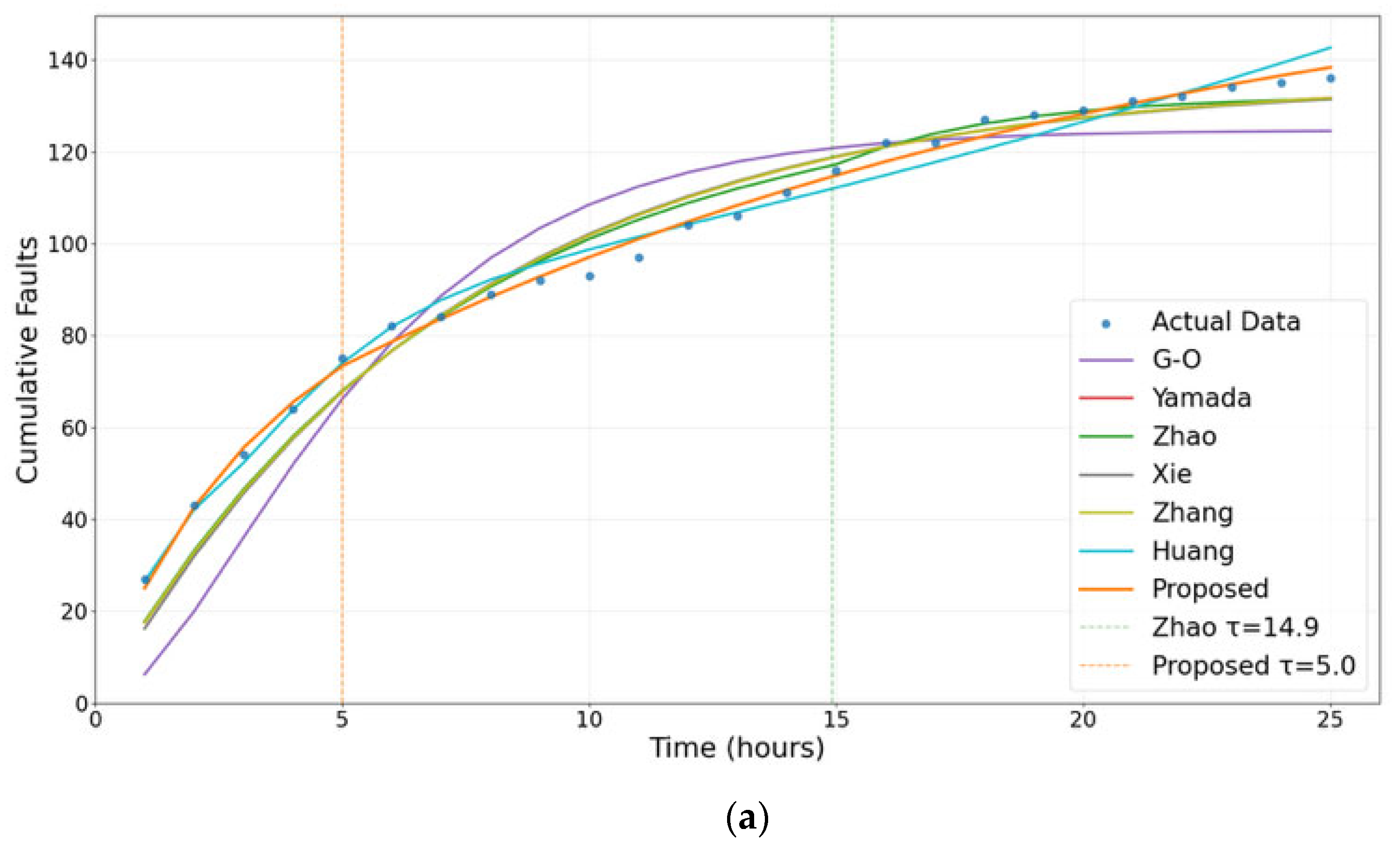
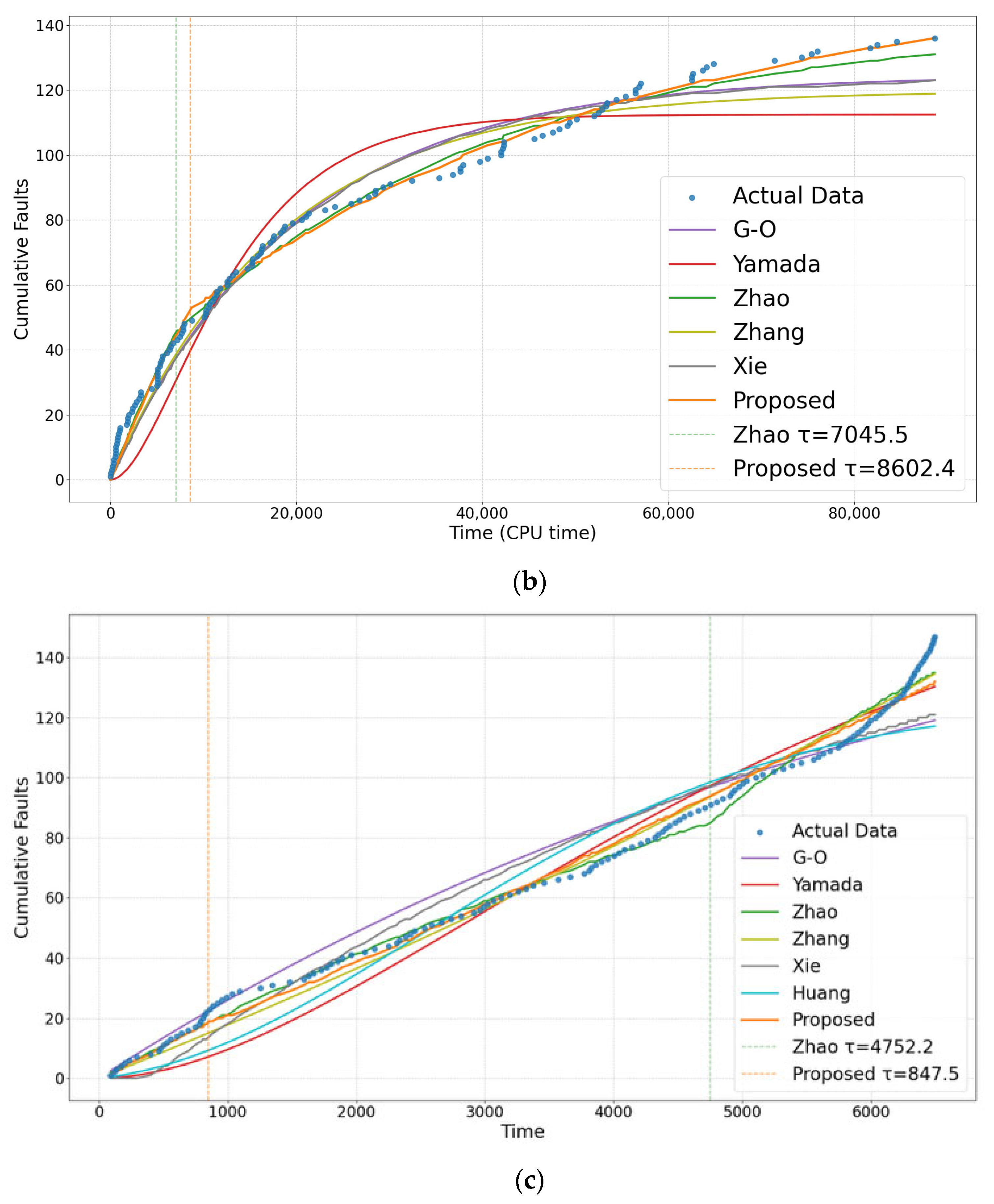
Figure 1 show the mean value function fitting graphs of the 6 models on DS1, DS2, and DS3, respectively.

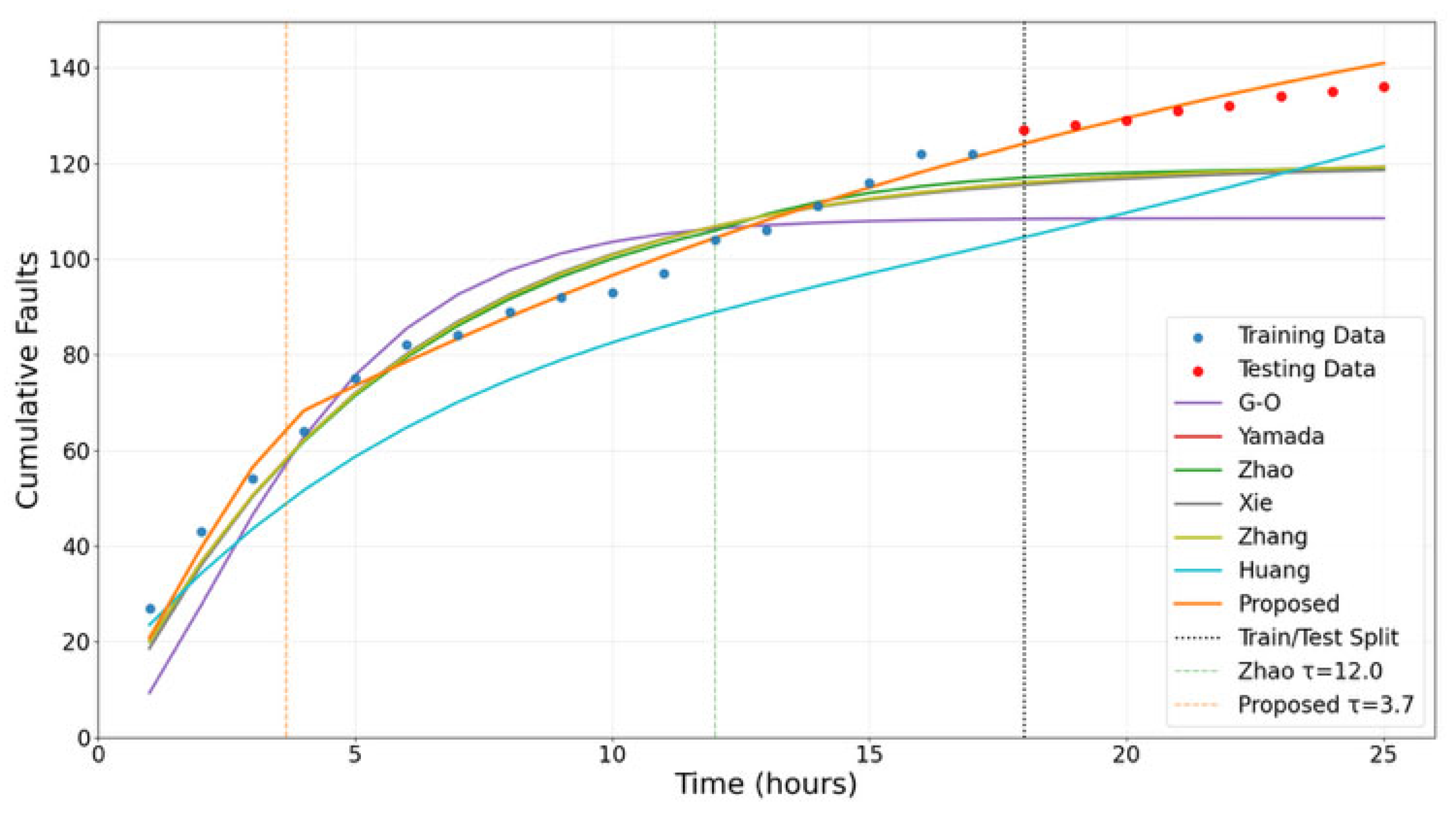
To further evaluate the predictive capability of the proposed model, an out-of-sample validation experiment was conducted. Specifically, the first 70% of the failure data were used for parameter estimation, while the remaining 30% were used for prediction evaluation.

Taking DS1 as an example, the fitting and prediction results of the proposed model are illustrated in Figure 2, while the corresponding evaluation results are summarized in

Table 6. Out-of-sample evaluation results of different models on DS1.

Model	MAE	SSE	AIC	RMSE	MAPE (%)
G–O	23.034	4320.4	54.333	23.239	17.471
Yamada	13.627	1519.8	49.974	13.783	10.331
Zhao	13.259	1457.7	49.642	13.498	9.043
Zhang	13.634	1521.4	53.984	13.791	10.337
Xie	14.202	1650.9	48.638	14.367	10.767
Huang	17.674	2577.3	56.200	17.949	13.504
Proposed	2.435	63.493	32.572	2.817	1.835

. It can be observed that the proposed model maintained good prediction accuracy not only on the training data but also on the unseen testing data. The predicted failure curve was generally consistent with the actual observed failure trend, indicating that the proposed model possesses satisfactory predictive capability for future software failures.

Furthermore, the experimental results demonstrate that the proposed model achieves relatively low prediction errors and stable performance across different evaluation metrics. This suggests that the model does not merely fit historical cumulative fault data, but also exhibits acceptable generalization capability in practical prediction scenarios. Therefore, the risk of over-fitting is considered limited.

3.4. Ablation and Sensitivity Analysis

To further investigate the contribution of different mechanisms in the proposed software reliability growth model, an ablation study was conducted by constructing several simplified variants of the complete model. The purpose of this analysis was to evaluate the influence of each component on the overall predictive performance of the model.

The detailed mechanisms retained in each ablation model are summarized in

Table 7. Configuration of different ablation models.

Model	Imperfect Debugging	Change-Point	Fault Classification	FDP–FCP
Full Model	✓	✓	✓	✓
Model A	✓	✗	✓	✓
Model B	✓	✓	✗$(p=0)$	✓
Model C	✓	✓	✗ ($p=1)$	✗

.

(1)

Full Model: The complete proposed model includes imperfect debugging, failure classification, FDP/FCP mechanisms, and change-point analysis.

(2)

Model A: Model A removes the change-point τ mechanism from the full model. It assumes that the software testing environment remains stable throughout the testing process, without abrupt parameter variations. Therefore, the fault detection rate and fault correction rate are treated as constant values rather than piecewise functions. The formula is shown as follows.

$$M_r\left(t\right)={\displaystyle \frac{A}{1-\alpha }}\left.\left(1-e^{-b\left(1-\alpha \right)t}\right.\right)+{\displaystyle \frac{A b\left(1-p\right)}{q-b\left(1-\alpha \right)}}\left.\left(e^{-qt}-e^{-b\left(1-\alpha \right)t}\right.\right)$$

(11)

(3)

Model B: Model B removes the fault diversity classification mechanism. In this case, all software faults are regarded as complex faults, and no instantly repairable simple faults are considered (i.e., the proportion coefficient of simple faults is set to $p=0)$. Consequently, all detected faults must undergo an independent delayed correction process. The formula is shown as follows.

$$M_r\left(t\right)=\left\{\begin{array}{c}{\displaystyle \frac{A}{1-\alpha }}\left.\left(1-e^{-b_1\left(1-\alpha \right)t}\right.\right)+{\displaystyle \frac{A b_1}{q_1-b_1\left(1-\alpha \right)}}\left.\left(e^{-q_{1}t}-e^{-b_1\left(1-\alpha \right)t}\right.\right), 0\le t\le \tau ,\\ {\displaystyle \frac{A}{1-\alpha }}\left.\left(1-e^{-b_1\left(1-\alpha \right)\tau -b_2\left(1-\alpha \right)\left(t-\tau \right)}\right.\right)+{\displaystyle \frac{A b_2}{q_2-b_2\left(1-\alpha \right)}}\left.\left(\begin{array}{c}{e}^{-q_1\tau -q_2\left(t-\tau \right)}-\\ e^{-b_1\left(1-\alpha \right)\tau -b_2\left(1-\alpha \right)\left(t-\tau \right)}\end{array}\right.\right)\\ +A\left.\left(e^{-q_1\tau }-e^{-b_1\left(1-\alpha \right)\tau }\right.\right)\left({\displaystyle \frac{b_1}{q_1-b_1\left(1-\alpha \right)}}-{\displaystyle \frac{b_2 }{q_2-b_2\left(1-\alpha \right)}}\right), t>\tau .\end{array}\right.$$

(12)

(4)

Model C: Model C removes the coupled FDP–FCP mechanism and returns to the traditional assumption that fault detection and fault correction occur synchronously. Under this assumption, no delayed correction process or pending fault accumulation exists after fault detection. Therefore, the correction quantity of complex faults satisfies $M_c\left(t\right)=0$, and the pending fault quantity becomes $B\left(t\right)=0$.

Since the delayed correction process is no longer considered, all software faults are treated as simple faults that can be repaired immediately after detection (i.e., the proportion coefficient is set to $p=1)$. Consequently, the fault diversity classification mechanism is also implicitly removed in this model.

This model still retains the change-point mechanism and imperfect debugging assumption. Accordingly, the cumulative removed faults are directly determined by the fault detection process. The simplified segmented mean value function is given as follows.

$$M_r\left(t\right)=\left\{\begin{array}{c}{\displaystyle \frac{A}{1-\alpha }}\left.\left(1-e^{-b_1\left(1-\alpha \right)t}\right.\right), 0\le t\le \tau ,\\ {\displaystyle \frac{A}{1-\alpha }}\left.\left(1-e^{-b_1\left(1-\alpha \right)\tau -b_2\left(1-\alpha \right)\left(t-\tau \right)}\right.\right), t>\tau .\end{array}\right.$$

(13)

Based on Model C, when the fault introduction effect caused by imperfect debugging is further ignored, namely $\alpha =0$, the proposed model degenerates into the traditional perfect debugging framework, where no new faults are introduced during the debugging process. Furthermore, if the change-point effect is also neglected, the fault detection rate remains constant throughout the entire testing process. In this case, the proposed model can be further simplified to the classical Goel–Okumoto (GO) software reliability growth model. Therefore, the GO model can be regarded as a special case of the proposed model without imperfect debugging and change-point effects.

The ablation experimental results shown in

Table 8. Ablation experimental results of different models on DS1.

Model	MAE	RMSE	MAPE	SSE	R2	AIC
Model A	1.802667	2.257413	1.973435	127.3978	0.994414	50.71096
Model B	2.280082	3.041885	3.592482	231.3266	0.989857	69.62387
Model C	2.054754	2.487199	2.816897	154.654	0.993219	55.55787
Full Model	1.713675	2.100619	1.941986	110.315	0.995163	53.1116

indicate that the full model generally achieved the best performance among all comparison models across most evaluation criteria, demonstrating the effectiveness of integrating the change-point mechanism, fault diversity classification, and the coupled FDP–FCP process into a unified framework.

Among the simplified variants, Model A, which removes the change-point mechanism, still maintained relatively good prediction performance and ranked second overall. This suggests that although the change-point effect contributes positively to the modeling accuracy, the remaining mechanisms can still capture the main characteristics of the software fault evolution process.

In comparison, the performances of Models B and C declined to different degrees after removing the fault diversity classification mechanism and the coupled FDP–FCP process. These results indicate that fault diversity and the interaction between fault detection and fault correction play important roles in describing the dynamic characteristics of practical software testing processes. Without these mechanisms, the models cannot effectively characterize the complexity of software fault evolution, resulting in reduced prediction accuracy.

Overall, the ablation results demonstrate that each introduced mechanism contributed positively to the predictive capability of the proposed model, while the complete model achieved the most stable and accurate performance.

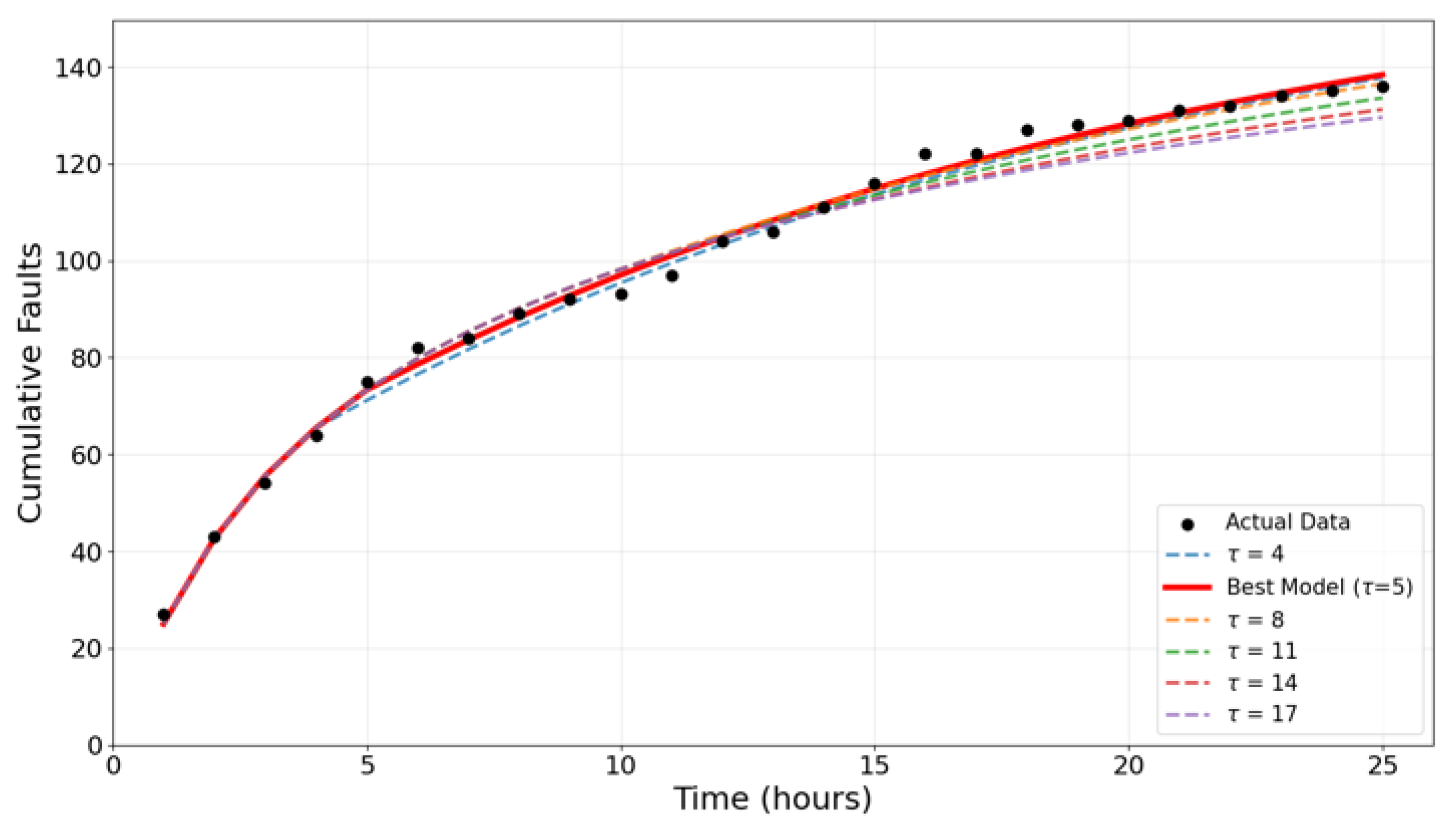
To further investigate the robustness and stability of the proposed model, a sensitivity analysis on the change-point parameter $\tau$ was conducted in this section. Since the change-point mechanism plays an important role in characterizing dynamic variations during the software testing process, different values of $\tau$ were selected to evaluate their influence on the prediction performance of the model. Figure 3 shows the fitting curves of the proposed model under different change-point parameters on DS1, reflecting how the model performs with varying τ values.

The sensitivity analysis results are summarized in

Table 9. Sensitivity analysis results of the change-point parameter τ on DS1.

τ	MAE	RMSE	MAPE	SSE
4	2.028785	2.497572	2.295171	155.9466
5	1.713675	2.100619	1.941987	110.315
8	2.000713	2.429478	2.22388	147.559
11	2.823332	3.27166	2.845826	267.594
14	3.555194	4.184085	3.409394	437.6643
17	3.978307	4.770896	3.732172	569.0362

. It can be observed that the evaluation indicators fluctuated only slightly under different values of the change-point parameter $\tau$. This indicates that the proposed model maintains relatively stable prediction performance when moderate parameter variations occur.

Although different change-point settings may lead to minor changes in prediction accuracy, the overall fitting and prediction capabilities of the model remain stable. Therefore, the proposed model demonstrates acceptable robustness and sensitivity stability with respect to the change-point parameter.

4. Software Optimal Release Strategy

Determining the optimal release strategy is a critical decision for software projects. Under the condition of limited resources in software development projects, how to achieve an acceptable level of software reliability at minimum cost is a key issue that needs to be urgently addressed before software release. Many papers [24,25,42] have conducted research on this issue.

4.1. Based on Reliability Criteria and Cost Model: Optimal Software Release Strategy

Assuming that the software is released at time $T$, the software reliability function based on the NHPP within the interval $\left(T,T+\Delta T\right)$ is as follows:

$$R\left(\Delta T|T\right)=e^{-\left[M_d\left(T+\Delta T\right)-M_r\left(T\right)\right]}$$

(14)

Among them, $\Delta T$ represents the observation time interval after software release, during which failure data are collected and analyzed.

Besides reliability requirements, we also need to consider the costs of the testing phase and the operation phase. The total cost model can be expressed as:

$$C\left(T\right)= c_{1}T+c_{2}p{M}_d\left(T\right)+c_3{M}_c\left(T\right)+c_4\left[M_d\left(T_{LC}\right)-M_{\mathrm{r}}\left(T\right)\right]$$

(15)

Among them, $T_{LC}$ denotes the software life cycle length; $c_1$ represents the unit time cost for fault detection in the testing phase (including labor, environment, and tool expenses); $c_2$ is the unit cost for simple fault repair in the testing phase (estimated from actual working hours and engineer wage standards); $c_3$ stands for the unit cost for complex fault repair in the testing phase (involving senior engineers, longer working hours, and regression testing overhead), and $c_4$ refers to the unit fault removal cost in the operation phase (comprehensively including maintenance labor, downtime losses, user compensation, and brand reputation impact).

Considering both the reliability requirements and total cost, our goal was to determine the optimal software release time $T$ to minimize the total life cycle cost while satisfying the pre-defined reliability constraint. The final optimization objective is: Min $C\left(T\right)$, The constraint conditions are: $R\left(\Delta T|T\right)=e^{-\left[M_d\left(T+\Delta T\right)-M_r\left(T\right)\right]}\ge R_1$, among them, $R_1$ denotes the minimum acceptable reliability target for software release.

4.2. Numerical Example of Software Release Strategy

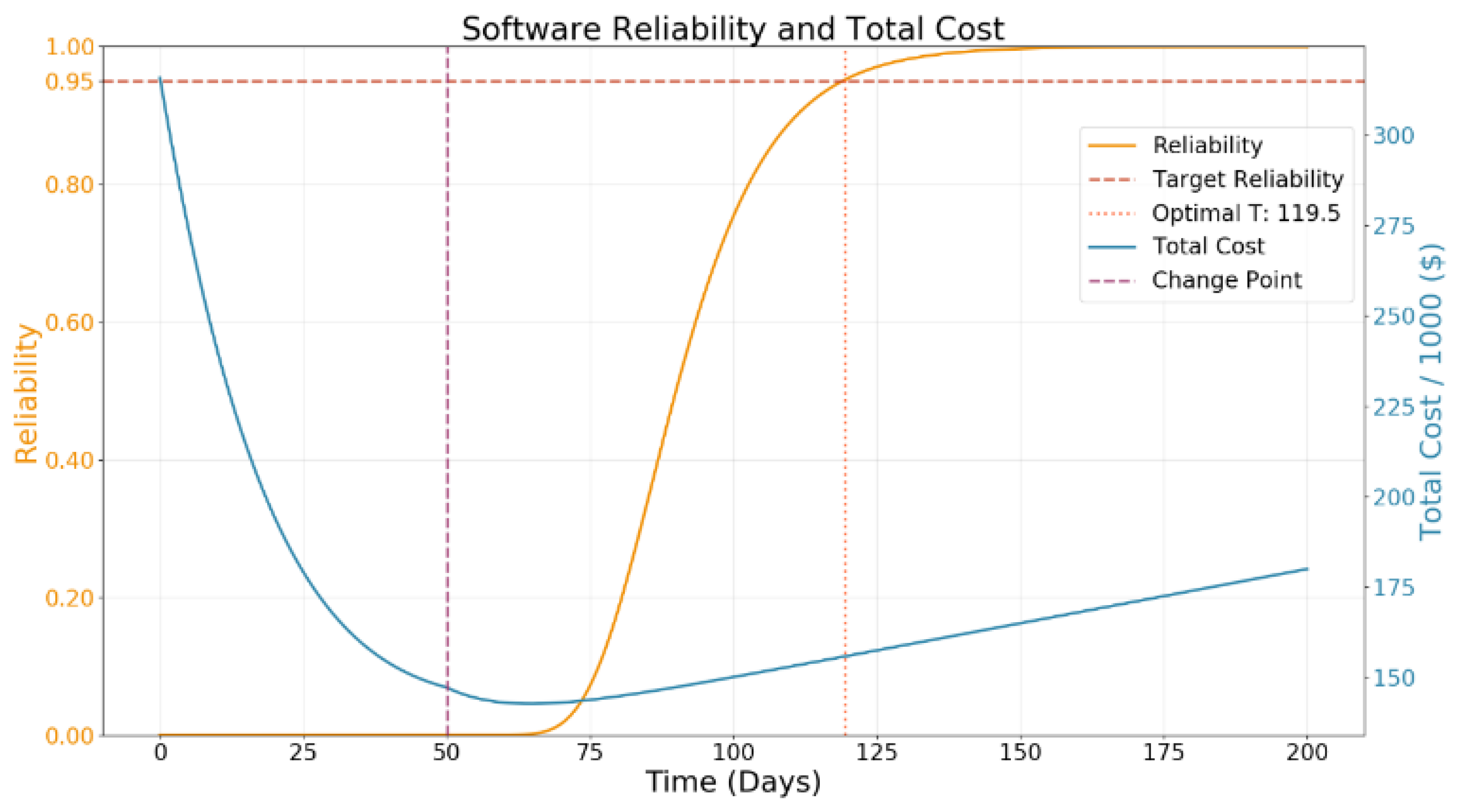
Suppose a software company has completed the development of a commercial system and is now in the final phase of the software development life cycle. At this critical juncture, the manager faces the crucial decision of determining the optimal release time for the commercial system. It is assumed that the fixed daily testing cost $c_1$ is USD 300; the unit cost for repairing simple faults $c_2$ and the unit cost for repairing complex faults $c_3$ in the testing phase are USD 200 and USD 500, respectively; the comprehensive cost caused by unit faults in the operation phase (including costs of detection, repair, as well as risks and reputation impacts) $c_4$ is USD 1000. The testing cycle $T_{LC}$ was set to 200 days; due to the increase in testers, the change point $\tau$ will occur on day 50. To meet customer requirements, the final software reliability $R_1$ needs to reach 0.95, and $\Delta T=10$.

Based on the test data of multiple typical software projects in the past, a systematic analysis of the parameters of the residual mean value function was conducted, and the estimated values were as follows: $A=300, p=0.4$, $\alpha$ = 0.05, $b_1$ = 0.1, $b_2$ = 0.15, $q_1=0.06$, $q_2=0.09$.

Figure 4 shows the changes in the total cost function C(T) and the reliability function R(ΔT|T) as a function of time. It can be seen that when the release time T ≥ 119.5, the reliability can meet the requirement of 0.95. On this basis, the release time T with the lowest cost is 119.5 days, and the minimum total cost C(T) is USD 155,874.56.

5. Conclusions and Future Research Suggestions

The construction of software reliability growth models, a crucial tool in the software development process, enables managers to scientifically predict software reliability metrics and systematically evaluate and monitor the software development process. Based on the analysis results of the model, managers can further optimize resource allocation plans, accurately determine the optimal release time of the software, and maximize development benefits.

This study focused on the limitations of software reliability growth models (SRGMs) in practical testing scenarios. By integrating elements such as imperfect debugging, the correlation between the fault detection process (FDP) and the fault correction process (FCP), fault diversity (distinguishing between simple and complex faults), and change points, a novel software reliability growth model based on the non-homogeneous Poisson Process (NHPP) is constructed. This model can more accurately depict the dynamic evolution process of software faults in actual testing environments, providing more realistic theoretical support for software reliability assessment.

Through parameter estimation using the least squares estimation (LSE) method and validation with three widely used datasets (DS1, DS2, DS3), the proposed model was compared with six representative SRGMs based on multiple evaluation indicators, including MAE, SSE, RMSE, MAPE, $R^2$, and AIC. The experimental results demonstrate that the proposed model generally achieves lower prediction errors and better overall performance across different datasets. In addition, the out-of-sample validation experiments further verify that the proposed model maintains satisfactory predictive capability on previously unseen data, indicating acceptable generalization ability and limited over-fitting risk.

To further evaluate the effectiveness of different mechanisms in the proposed model, ablation experiments and sensitivity analyses were also conducted. The results indicate that the change-point mechanism, fault diversity classification, and coupled FDP–FCP process all contribute positively to the prediction accuracy and robustness of the proposed model. These findings further confirm the rationality and effectiveness of incorporating multiple practical testing factors into the software reliability modeling framework.

Based on the proposed reliability model, this study further establishes a software cost-reliability optimization framework that simultaneously considers the testing phase costs and operational phase risk costs. A numerical example demonstrated that the proposed release strategy can minimize the total expected cost while satisfying the preset reliability requirement. Therefore, the proposed framework can provide project managers with a quantitative decision-making basis for balancing software reliability and development cost.

In addition, the proposed model is independent of specific software development methodologies and can also be applied to iterative development environments such as Agile or Scrum. In practical software repositories and issue tracking systems (e.g., Jira), the cumulative fault data and model parameters may be estimated from defect reports, issue state transitions, debugging logs, and testing records collected during software testing and maintenance processes.

Nevertheless, the proposed model still has certain practical limitations. The current study was mainly validated using publicly available benchmark datasets, and the diversity of industrial software projects remains relatively limited. In addition, some model assumptions, such as fixed fault classification proportions and predefined change-point settings, may not fully reflect the highly dynamic characteristics of real-world software development environments. Therefore, the applicability of the proposed model to large-scale and highly complex industrial software systems still requires further investigation.

Future research can be extended in several directions. First, the current model assumes a single known change point, whereas practical software testing processes may involve multiple unknown change points caused by continuous adjustments in testing strategies, personnel, and testing tools. Second, time-varying fault detection and correction rates may be introduced to better characterize the dynamic evolution of testing efficiency throughout the software life cycle. Third, more refined fault classification mechanisms based on fault severity, repair difficulty, and system impact can be considered to further improve the modeling accuracy. Fourth, future work may further consider more complex real-world software engineering factors, such as successive software version releases, evolving requirement changes, repository issue handling states, and the influence of continuously generated event logs during testing and operational phases. Finally, additional practical factors, such as maintenance cost, warranty cost, and operational uncertainty, may be incorporated to establish a more comprehensive software reliability optimization framework.