Author Contributions
Conceptualization, R.V.C.; methodology, R.V.C.; software, R.V.C.; validation, R.V.C. and A.M.; formal analysis, R.V.C.; investigation, A.M.; resources, R.V.C. and A.M.; data curation, R.V.C.; writing—original draft preparation, R.V.C.; writing—review and editing, A.M.; visualization, R.V.C.; supervision, A.M.; project administration, A.M.; funding acquisition, A.M. All authors have read and agreed to the published version of the manuscript.
Figure 1.
Transfer learning pipeline for intrusion detection. Tabular network flow features are scaled, padded, and reshaped into a single-channel image for classification by a pre-trained CNN architecture.
Figure 1.
Transfer learning pipeline for intrusion detection. Tabular network flow features are scaled, padded, and reshaped into a single-channel image for classification by a pre-trained CNN architecture.
Figure 2.
Lab experiment network topology. The Attacker node replays CICIDS2017 PCAP captures over an isolated Ethernet segment to the Sniffer node via a SPAN-mirrored switch. The Sniffer node (Raspberry Pi 4) simulates a resource-constrained edge device hosting the IDS. A host workstation (not depicted) connects over WiFi for out-of-band administrative control of both nodes and is not part of the IDS data path.
Figure 2.
Lab experiment network topology. The Attacker node replays CICIDS2017 PCAP captures over an isolated Ethernet segment to the Sniffer node via a SPAN-mirrored switch. The Sniffer node (Raspberry Pi 4) simulates a resource-constrained edge device hosting the IDS. A host workstation (not depicted) connects over WiFi for out-of-band administrative control of both nodes and is not part of the IDS data path.
Figure 3.
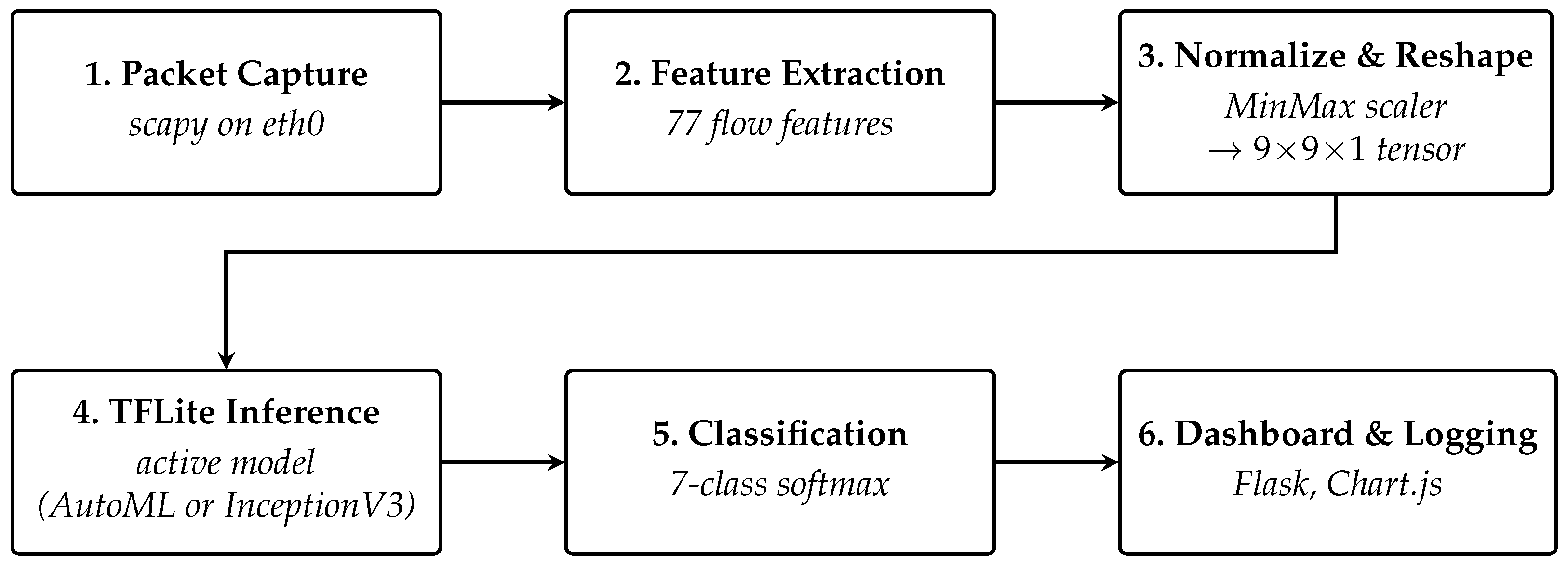
Onboard inference pipeline on the Sniffer/IDS node. Captured packets are converted to flow-level features (77
CICIDS2017 features), normalized with the migrated MinMax scaler, reshaped to a
tensor, classified by the currently selected TFLite model (AutoML: 1.18 M parameters, ∼3 ms per inference; or InceptionV3: 22.3 M parameters, ∼85 ms; sizes reported in
Section 4.3.4) into one of the seven
CICIDS2017 attack classes (BENIGN, Bot, BruteForce, DoS, Infiltration, PortScan, WebAttack), and logged to a Flask dashboard. A co-located System Monitor samples CPU utilization, memory consumption, and die temperature at one-second intervals (
Section 4).
Figure 3.
Onboard inference pipeline on the Sniffer/IDS node. Captured packets are converted to flow-level features (77
CICIDS2017 features), normalized with the migrated MinMax scaler, reshaped to a
tensor, classified by the currently selected TFLite model (AutoML: 1.18 M parameters, ∼3 ms per inference; or InceptionV3: 22.3 M parameters, ∼85 ms; sizes reported in
Section 4.3.4) into one of the seven
CICIDS2017 attack classes (BENIGN, Bot, BruteForce, DoS, Infiltration, PortScan, WebAttack), and logged to a Flask dashboard. A co-located System Monitor samples CPU utilization, memory consumption, and die temperature at one-second intervals (
Section 4).
Figure 4.
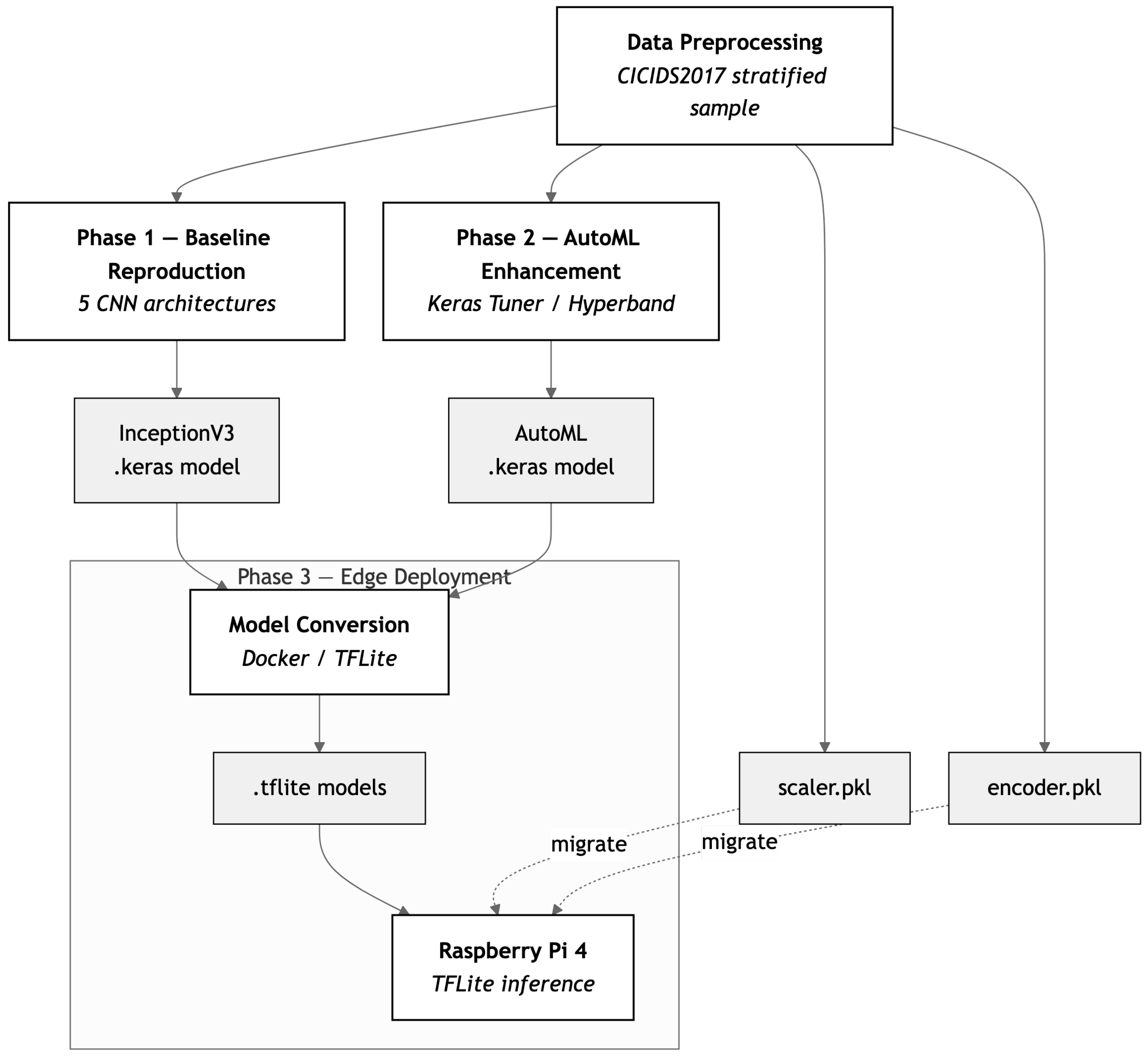
Preprocessing state migration from training to edge deployment. Data preprocessing produces the shared
scaler.pkl and
encoder.pkl artifacts that are consumed by both Phase 1 (baseline reproduction) and Phase 2 (AutoML enhancement). Phase 3 encompasses the full edge deployment workflow: the resulting
.keras models from both phases are converted to TFLite format via Docker and deployed to the Raspberry Pi 4, while the serialized scaler and encoder are migrated directly to the Pi alongside the converted models. Classification integrity of the conversion process is validated during this phase (see
Section 4.3.1).
Figure 4.
Preprocessing state migration from training to edge deployment. Data preprocessing produces the shared
scaler.pkl and
encoder.pkl artifacts that are consumed by both Phase 1 (baseline reproduction) and Phase 2 (AutoML enhancement). Phase 3 encompasses the full edge deployment workflow: the resulting
.keras models from both phases are converted to TFLite format via Docker and deployed to the Raspberry Pi 4, while the serialized scaler and encoder are migrated directly to the Pi alongside the converted models. Classification integrity of the conversion process is validated during this phase (see
Section 4.3.1).
Figure 5.
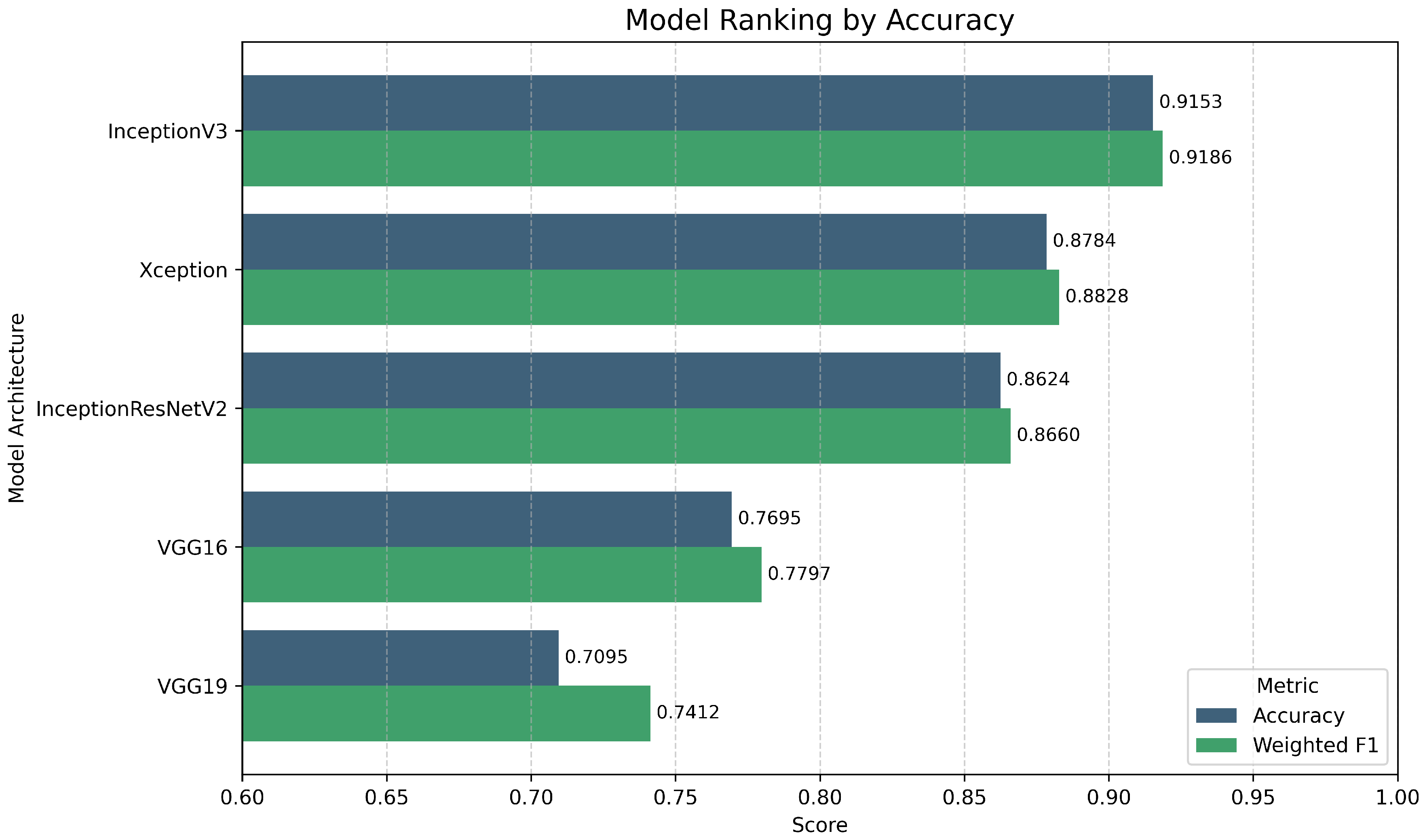
Comparison of model accuracy and Weighted F1-Score across all replicated deep learning architectures. InceptionV3 is the top-performing baseline.
Figure 5.
Comparison of model accuracy and Weighted F1-Score across all replicated deep learning architectures. InceptionV3 is the top-performing baseline.
Figure 6.
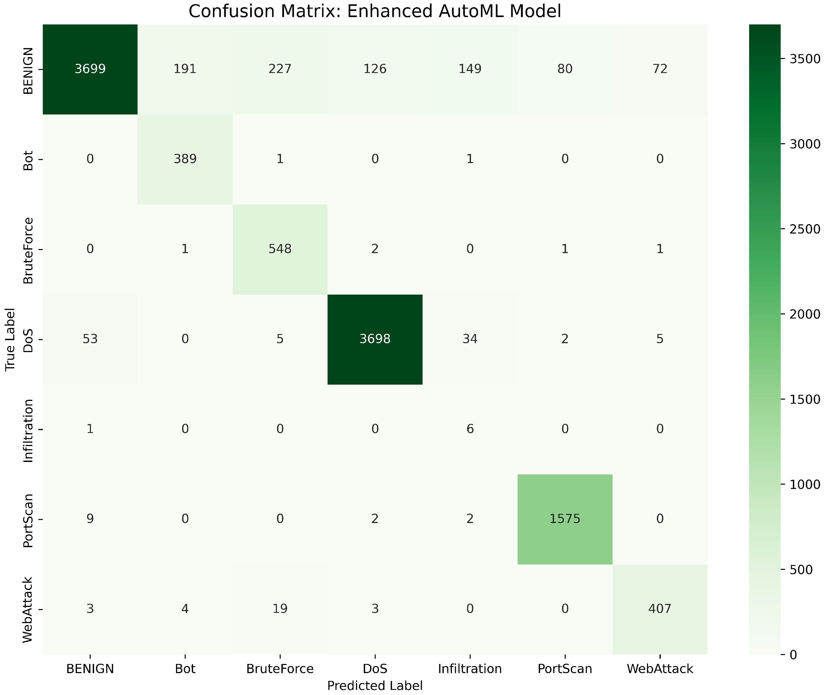
Confusion matrix for the AutoML enhanced model on the CICIDS2017 test set.
Figure 6.
Confusion matrix for the AutoML enhanced model on the CICIDS2017 test set.
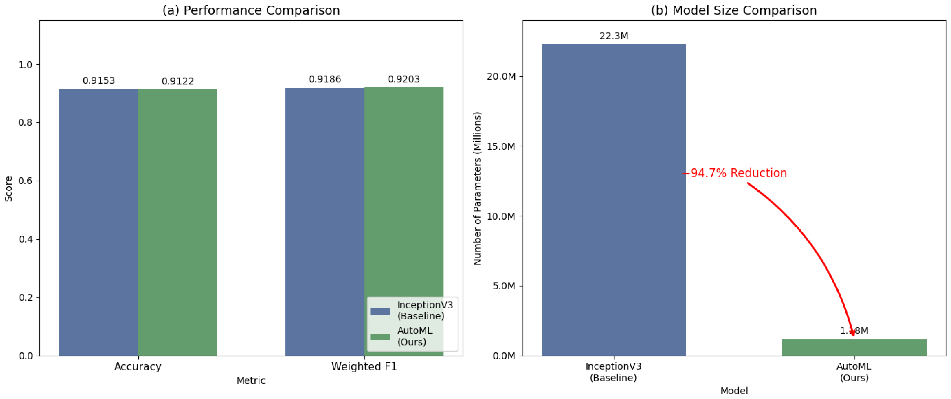
Figure 7.
Performance and model size comparison between the InceptionV3 baseline and the AutoML-optimized model. (a) Classification performance (Accuracy and Weighted F1) of both models, where higher is better. (b) Trainable parameter count of both models in millions, where lower is better; the AutoML model achieves a 94.7% reduction relative to the InceptionV3 baseline.
Figure 7.
Performance and model size comparison between the InceptionV3 baseline and the AutoML-optimized model. (a) Classification performance (Accuracy and Weighted F1) of both models, where higher is better. (b) Trainable parameter count of both models in millions, where lower is better; the AutoML model achieves a 94.7% reduction relative to the InceptionV3 baseline.
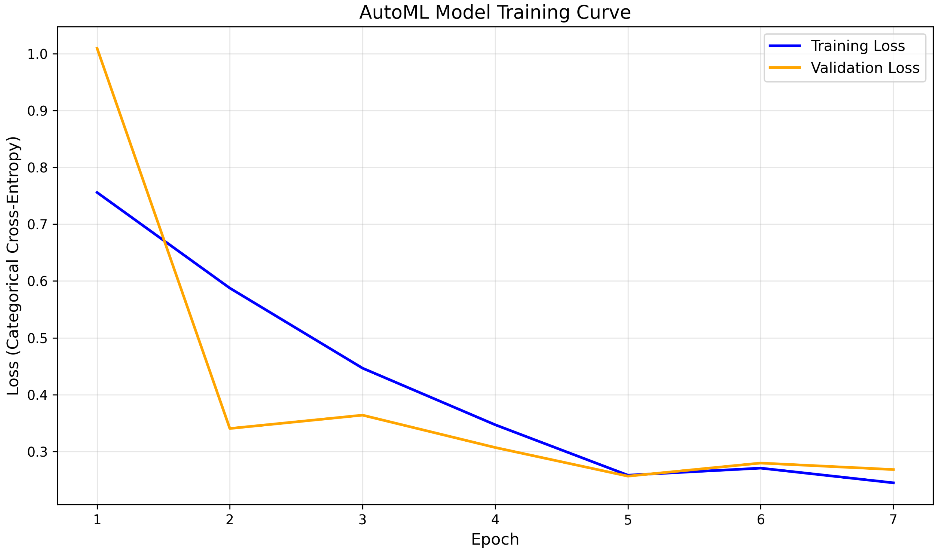
Figure 8.
AutoML model training and validation loss curves across all training epochs.
Figure 8.
AutoML model training and validation loss curves across all training epochs.
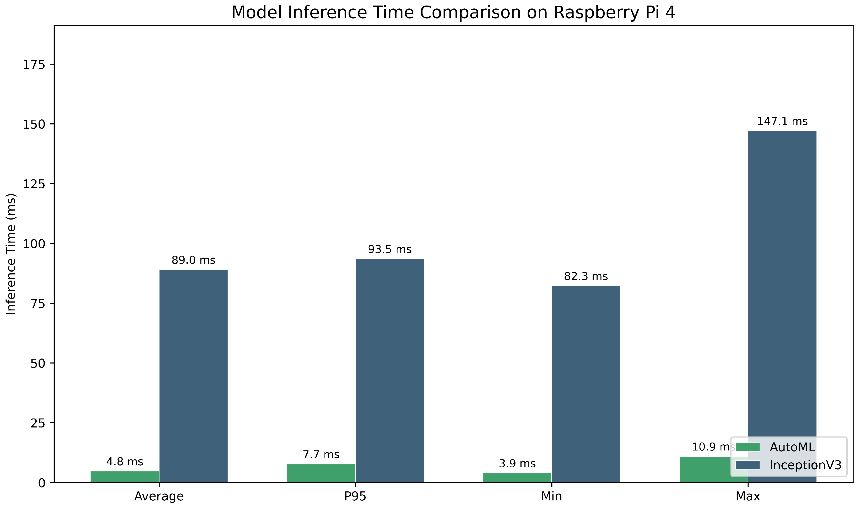
Figure 9.
Inference latency comparison under sustained PCAP replay load on Raspberry Pi 4. AutoML achieves an 18.7× speedup over InceptionV3 across all latency percentiles.
Figure 9.
Inference latency comparison under sustained PCAP replay load on Raspberry Pi 4. AutoML achieves an 18.7× speedup over InceptionV3 across all latency percentiles.
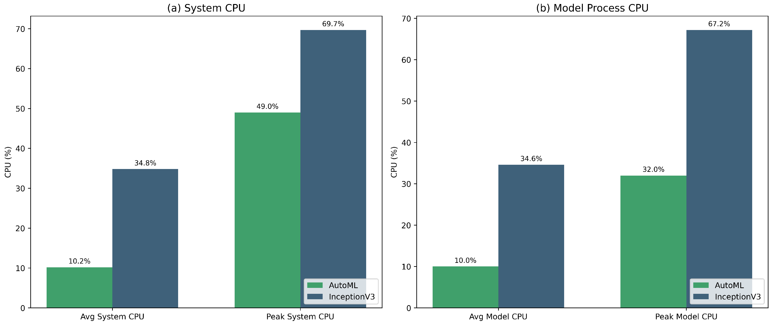
Figure 10.
CPU utilization comparison on the Raspberry Pi 4. (a) System wide CPU utilization (average and peak). (b) Model process CPU utilization (average and peak). The AutoML model requires approximately 3.5× less CPU than InceptionV3 for sustained IDS inference.
Figure 10.
CPU utilization comparison on the Raspberry Pi 4. (a) System wide CPU utilization (average and peak). (b) Model process CPU utilization (average and peak). The AutoML model requires approximately 3.5× less CPU than InceptionV3 for sustained IDS inference.
Figure 11.
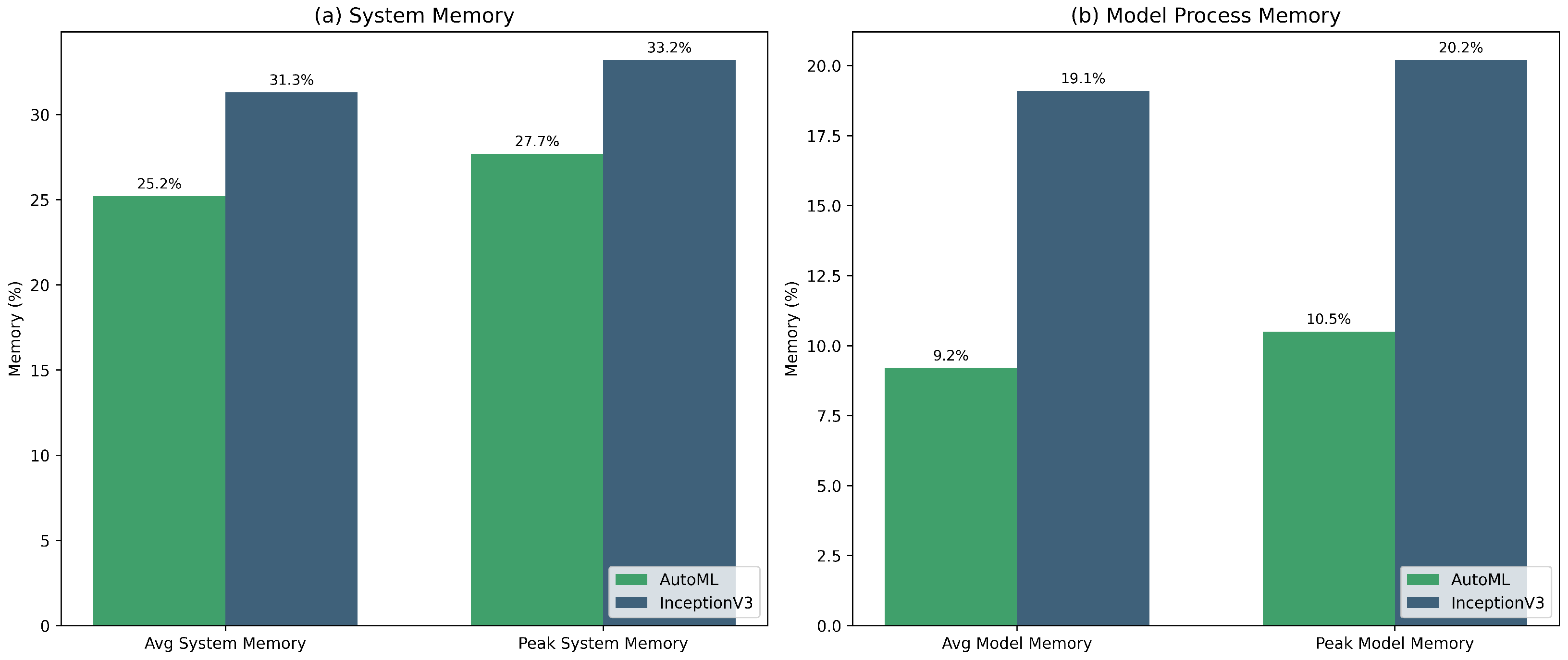
Memory utilization comparison on the Raspberry Pi 4. (a) System-wide memory utilization (average and peak). (b) Model process memory utilization (average and peak). The AutoML model requires approximately 2.1× less memory than InceptionV3 for sustained IDS inference.
Figure 11.
Memory utilization comparison on the Raspberry Pi 4. (a) System-wide memory utilization (average and peak). (b) Model process memory utilization (average and peak). The AutoML model requires approximately 2.1× less memory than InceptionV3 for sustained IDS inference.
Figure 12.
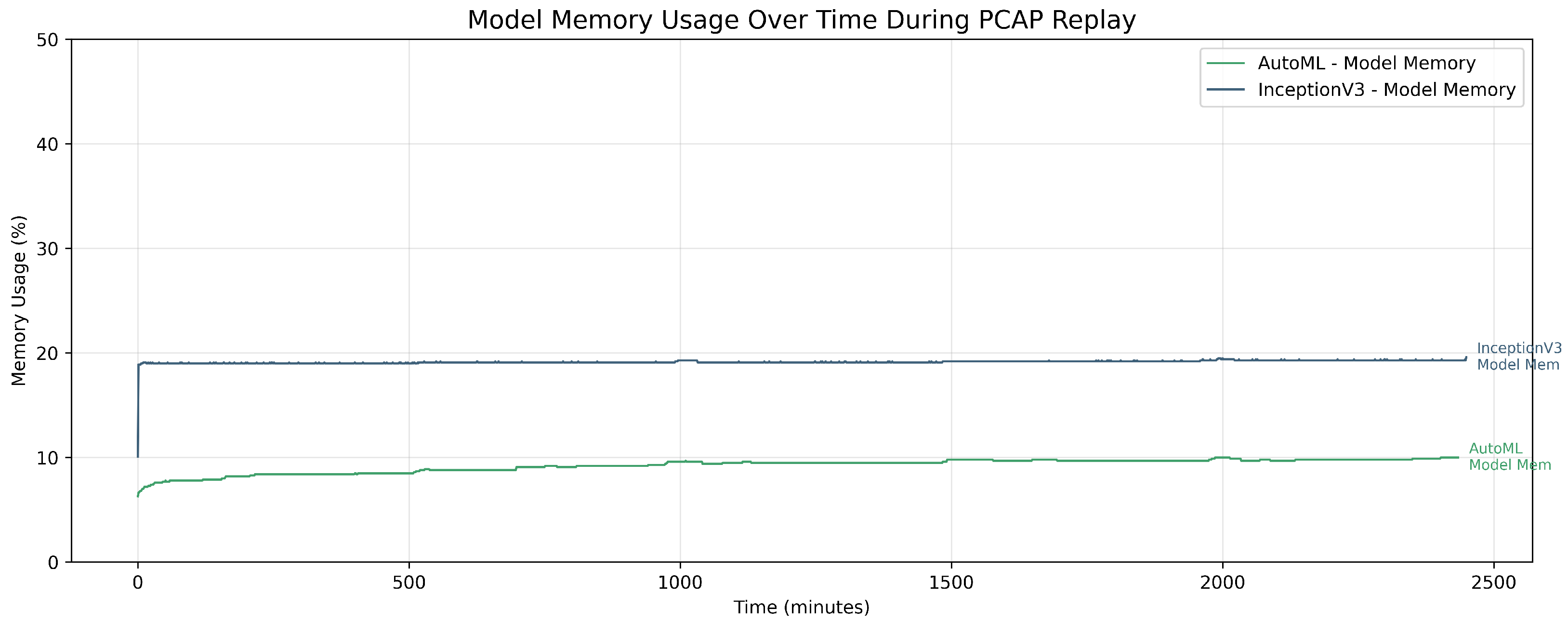
Model memory usage over time during the 41 h PCAP replay. Both models maintain stable memory profiles with no evidence of memory leaks.
Figure 12.
Model memory usage over time during the 41 h PCAP replay. Both models maintain stable memory profiles with no evidence of memory leaks.
Figure 13.
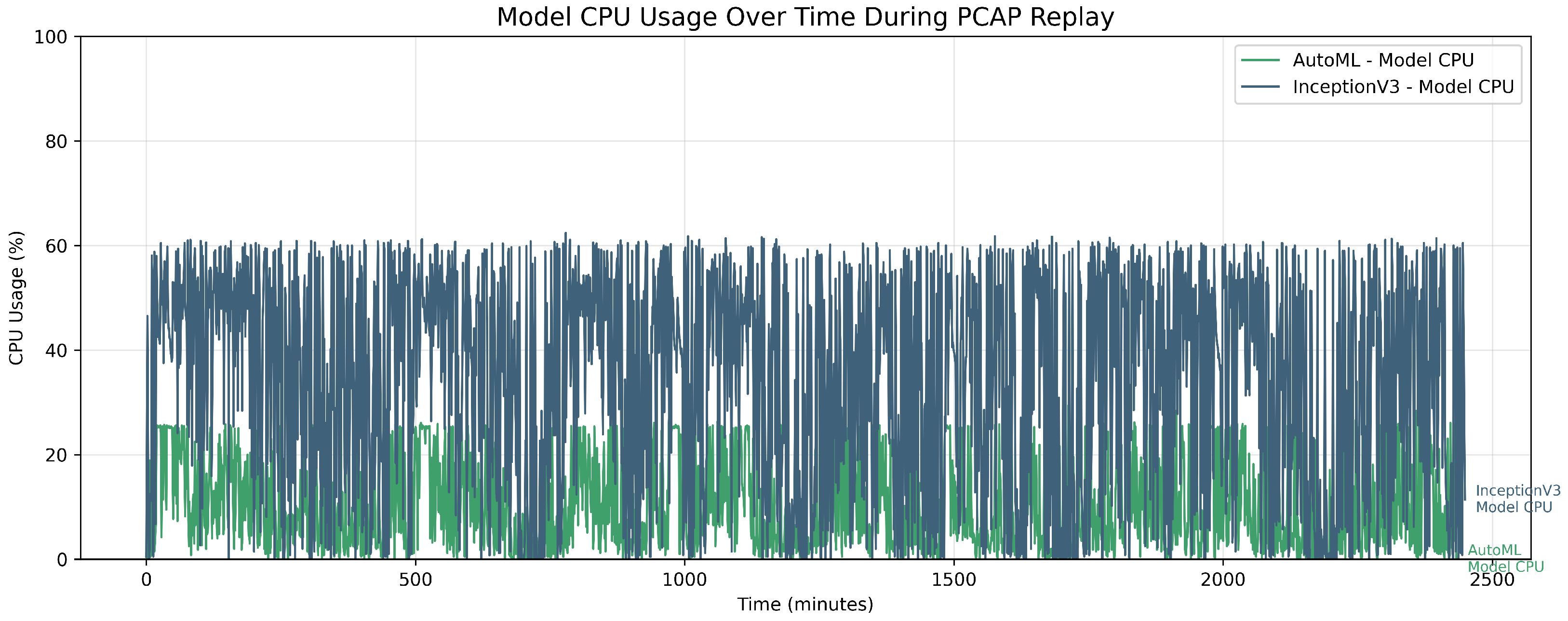
Model CPU usage over time during PCAP replay. InceptionV3 sustains 3.5× higher CPU load throughout the 41 h test.
Figure 13.
Model CPU usage over time during PCAP replay. InceptionV3 sustains 3.5× higher CPU load throughout the 41 h test.
Figure 14.
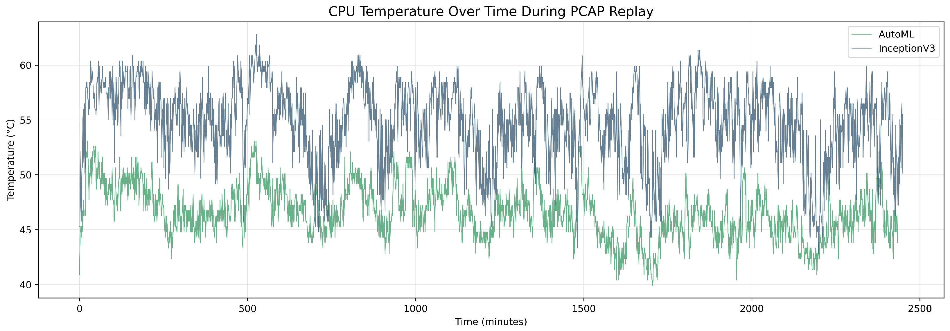
CPU temperature over time during PCAP replay. InceptionV3 induces higher sustained thermal load on the passively cooled ARM processor.
Figure 14.
CPU temperature over time during PCAP replay. InceptionV3 induces higher sustained thermal load on the passively cooled ARM processor.
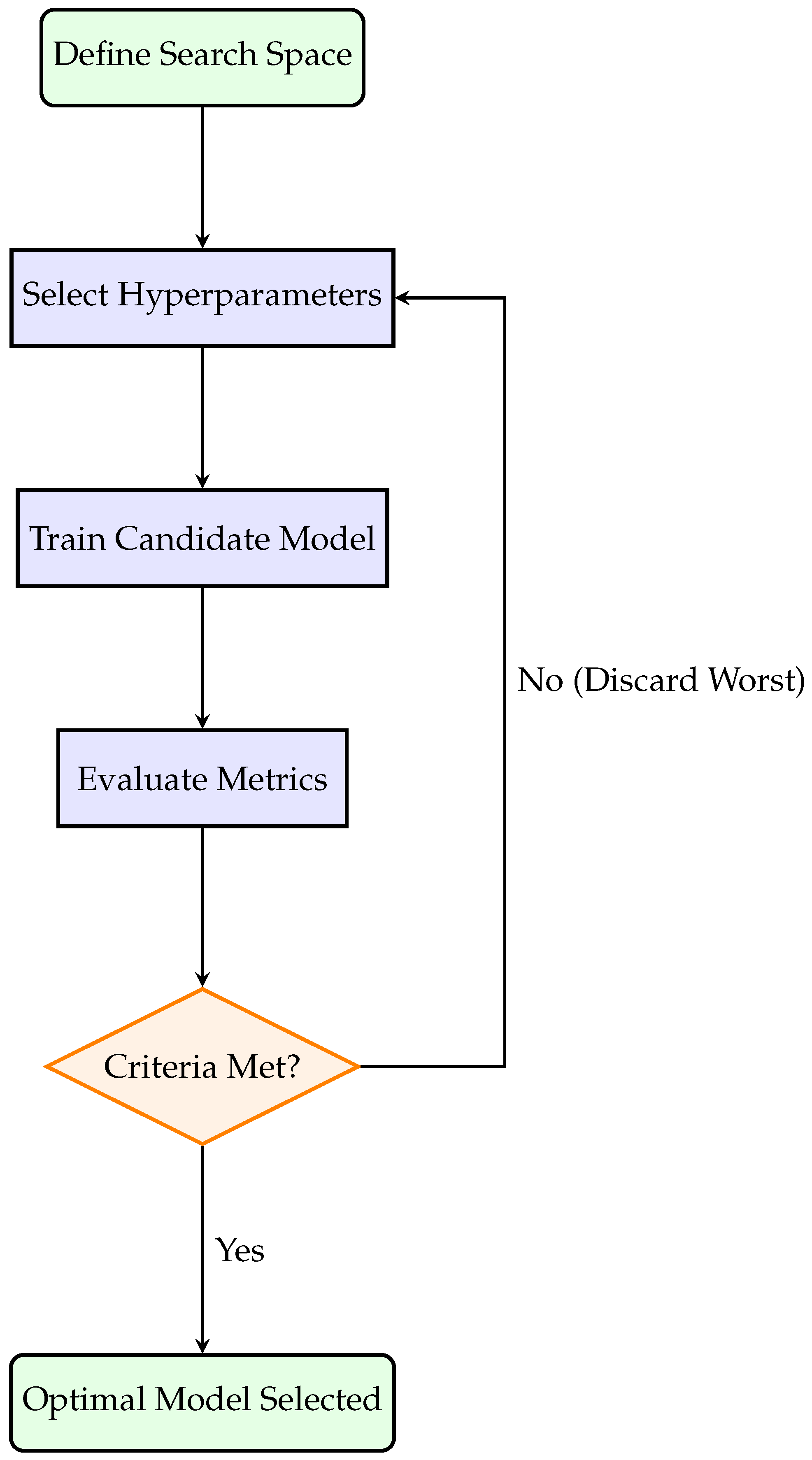
Figure 15.
The AutoML optimization loop: The Hyperband algorithm iteratively selects hyperparameters, trains candidates, and progressively discards the worst performers to minimize model size while maximizing accuracy.
Figure 15.
The AutoML optimization loop: The Hyperband algorithm iteratively selects hyperparameters, trains candidates, and progressively discards the worst performers to minimize model size while maximizing accuracy.
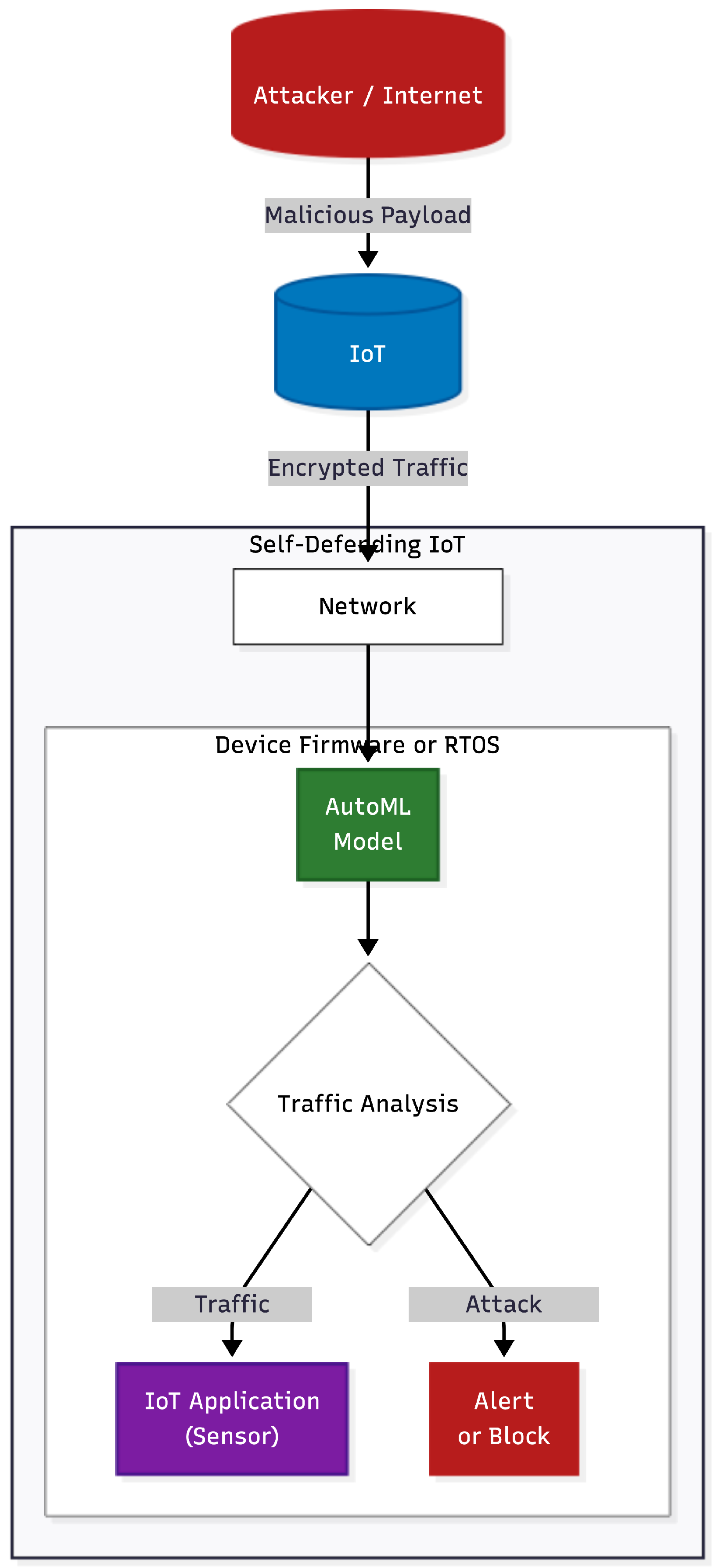
Figure 16.
Proposed embedded HIDS architecture. The AutoML model runs directly on the device firmware to inspect traffic after decryption.
Figure 16.
Proposed embedded HIDS architecture. The AutoML model runs directly on the device firmware to inspect traffic after decryption.
Table 1.
Positioning of this work relative to recent deep learning IDS research. “Reported Acc.” is each cited paper’s own best result on the dataset it used; these figures are not directly comparable across rows, since the datasets, splits, and evaluation protocols differ, and are listed only to confirm that the surveyed methods are strong, well-regarded detectors. The comparison this table draws is along the model-size (“Params”) and edge-validation columns. “N/R” denotes a value not reported in a directly comparable form in the cited work; “(F1)” marks an F1-score rather than accuracy.
Table 1.
Positioning of this work relative to recent deep learning IDS research. “Reported Acc.” is each cited paper’s own best result on the dataset it used; these figures are not directly comparable across rows, since the datasets, splits, and evaluation protocols differ, and are listed only to confirm that the surveyed methods are strong, well-regarded detectors. The comparison this table draws is along the model-size (“Params”) and edge-validation columns. “N/R” denotes a value not reported in a directly comparable form in the cited work; “(F1)” marks an F1-score rather than accuracy.
| Work | Architecture | Dataset | Params | Reported Acc. | Edge-Validated |
|---|
| RTIDS [19] | Transformer | CICIDS2017 | N/R | 99.17% (F1) | No |
| Yang et al. [21] | Vision Transformer | NSL-KDD | N/R | 99.68% | No |
| FlowTransformer [20] | Transformer a | UNSW-NB15 a | varies a | ∼0.97 (F1) a | No |
| Gueriani et al. (2024) [22] | CNN-LSTM | CICIoT2023 | N/R | 98.42% | No |
| Gueriani et al. (2025) [12] | LSTM-CNN-Attention | Edge-IIoTset | N/R | 99.04% | No |
| This work (AutoML) | Compact CNN | CICIDS2017 | 1.18 M | 91.22% | Yes (Pi 4) |
Table 2.
AutoML search space and hyperband configuration.
Table 2.
AutoML search space and hyperband configuration.
| Hyperparameter | Type | Range/Choices |
|---|
| Searched (8 tunable hyperparameters) |
| img_size | Choice | {32, 48} |
| conv_blocks | Int | 1–3 |
| filters_i | Int | 16–64, step 16 (per block) |
| batch_norm | Boolean | {True, False} |
| conv_dropout | Float | 0.0–0.3, step 0.1 |
| dense_units | Int | 32–128, step 32 |
| dense_dropout | Float | 0.2–0.5, step 0.1 |
| learning_rate | Choice | {, } |
| Hyperband configuration |
| Objective | — | val_accuracy |
| Max epochs per trial | — | 12 |
| Reduction factor | — | 3 |
| Early stopping | — | monitor = val_loss, patience = 2 |
| Class weights | — | balanced (per training distribution) |
| Final retrain epochs | — | 10 |
| Fixed (not searched) |
| Optimizer | — | Adam |
| Loss | — | Categorical cross-entropy |
| Kernel size | — | , padding = same |
| Pooling | — | MaxPooling |
| Hidden activation | — | ReLU |
| Output activation | — | Softmax |
Table 3.
Edge testbed hardware specifications for Sniffer/IDS node (Raspberry Pi 4 Model B).
Table 3.
Edge testbed hardware specifications for Sniffer/IDS node (Raspberry Pi 4 Model B).
| Component | Specification |
|---|
| Processor (CPU) | Broadcom BCM2711, Quad-core Cortex A72 (ARM v8) 64-bit |
| Clock Speed | 1.5 GHz |
| Memory (RAM) | 2 GB LPDDR4-3200 SDRAM |
| Storage | 32 GB MicroSDHC (Class 10) |
| Network Interface | Gigabit Ethernet, 2.4 GHz and 5.0 GHz IEEE 802.11ac wireless |
| Operating System | Raspbian GNU/Linux 12 (Bookworm), 64-bit kernel (aarch64) running 32-bit armhf userspace, Kernel 6.12.75 |
Table 4.
Comparison of replicated deep learning architectures on CICIDS2017.
Table 4.
Comparison of replicated deep learning architectures on CICIDS2017.
| Model | Accuracy | Weighted F1 | Parameters |
|---|
| VGG16 | 0.7695 | 0.7797 | 14,847,845 |
| VGG19 | 0.7095 | 0.7412 | 20,157,541 |
| Xception | 0.8784 | 0.8828 | 21,387,853 |
| InceptionV3 | 0.9153 | 0.9186 | 22,329,157 |
| InceptionResNetV2 | 0.8624 | 0.8660 | 54,732,037 |
Table 5.
AutoML enhancement performance by class on CICIDS2017 test set.
Table 5.
AutoML enhancement performance by class on CICIDS2017 test set.
| Class | Precision | Recall | F1-Score | Support |
|---|
| BENIGN | 0.9825 | 0.8140 | 0.8904 | 4544 |
| Bot | 0.6650 | 0.9949 | 0.7971 | 391 |
| BruteForce | 0.6850 | 0.9910 | 0.8101 | 553 |
| DoS | 0.9653 | 0.9739 | 0.9696 | 3797 |
| Infiltration | 0.0312 | 0.8571 | 0.0603 | 7 |
| PortScan | 0.9499 | 0.9918 | 0.9704 | 1588 |
| WebAttack | 0.8392 | 0.9335 | 0.8838 | 436 |
| Overall Accuracy | 0.9122 | 11,316 |
Table 6.
Detailed confusion metrics by class (derived from confusion matrix). The FP and FN column totals are necessarily equal in single-label multi-class classification: each misclassified sample contributes one false negative to its true class and one false positive to its predicted class.
Table 6.
Detailed confusion metrics by class (derived from confusion matrix). The FP and FN column totals are necessarily equal in single-label multi-class classification: each misclassified sample contributes one false negative to its true class and one false positive to its predicted class.
| Class | Support | TP | FP | FN | Detection |
|---|
| (Total) | (Correct) | (False Alarm) | (Missed) | Rate (Recall) |
|---|
| BENIGN | 4544 | 3699 | 66 | 845 | 81.40% |
| Bot | 391 | 389 | 196 | 2 | 99.49% |
| BruteForce | 553 | 548 | 252 | 5 | 99.10% |
| DoS | 3797 | 3698 | 133 | 99 | 97.39% |
| Infiltration | 7 | 6 | 186 | 1 | 85.71% |
| PortScan | 1588 | 1575 | 83 | 13 | 99.18% |
| WebAttack | 436 | 407 | 78 | 29 | 93.35% |
| Totals | 11,316 | 10,322 | 994 | 994 | – |
Table 7.
Binary classification view of the AutoML model (BENIGN vs. Attack), derived directly from
Table 6 by collapsing the six attack classes into a single positive class.
Table 7.
Binary classification view of the AutoML model (BENIGN vs. Attack), derived directly from
Table 6 by collapsing the six attack classes into a single positive class.
| | Predicted: Attack | Predicted: BENIGN | Total |
|---|
| Actual: Attack | 6706 (TP) | 66 (FN) | 6772 |
| Actual: BENIGN | 845 (FP) | 3699 (TN) | 4544 |
| Total | 7551 | 3765 | 11,316 |
| Attack class metrics | Benign class metrics |
| Precision | 0.8881 | Specificity (TNR) | 0.8140 |
| Recall (TPR) | 0.9903 | False Positive Rate | 0.1860 |
| F1-Score | 0.9365 | False Negative Rate | 0.0097 |
| Overall Binary Accuracy: 0.9195 |
Table 8.
Efficiency comparison: replicated baseline vs. AutoML enhancement.
Table 8.
Efficiency comparison: replicated baseline vs. AutoML enhancement.
| Model | Accuracy | Weighted F1 | Parameters | Size Reduction |
|---|
| Replication (InceptionV3) | 0.9153 | 0.9186 | 22,329,157 | — |
| AutoML (Ours) | 0.9122 | 0.9203 | 1,180,615 | −94.7% |
Table 9.
Statistical comparison of the AutoML and InceptionV3 models on the 11,316-sample CICIDS2017 test set, computed from the existing test predictions (no retraining). Brackets give bootstrap 95% confidence intervals ( resamples).
Table 9.
Statistical comparison of the AutoML and InceptionV3 models on the 11,316-sample CICIDS2017 test set, computed from the existing test predictions (no retraining). Brackets give bootstrap 95% confidence intervals ( resamples).
| Metric | AutoML | InceptionV3 |
|---|
| Accuracy | 0.9122 | 0.9153 |
| Weighted F1 | 0.9203 | 0.9186 |
| Accuracy (AutoML − InceptionV3): , 95% CI |
| Weighted F1 (AutoML − InceptionV3): , 95% CI |
| McNemar’s test on paired predictions: , discordant; exact two-sided |
Table 10.
TFLite conversion integrity: Colab Keras vs. Raspberry Pi 4 TFLite.
Table 10.
TFLite conversion integrity: Colab Keras vs. Raspberry Pi 4 TFLite.
| Model | Env. | Accuracy | Weighted F1 | Conversion Loss |
|---|
| AutoML | Colab (Keras) | 0.9122 | 0.9203 | — |
| AutoML | Pi 4 (TFLite) | 0.9122 | 0.9203 | 0.00% |
| InceptionV3 | Colab (Keras) | 0.9153 | 0.9186 | — |
| InceptionV3 | Pi 4 (TFLite) | 0.9153 | 0.9186 | 0.00% |
Table 11.
Per-class conversion validation: AutoML Keras (Colab) vs. TFLite (Pi 4).
Table 11.
Per-class conversion validation: AutoML Keras (Colab) vs. TFLite (Pi 4).
| Class | Keras Precision | TFLite Precision | Keras Recall | TFLite Recall | Keras F1 | TFLite F1 |
|---|
| BENIGN | 0.9825 | 0.9825 | 0.8140 | 0.8140 | 0.8904 | 0.8904 |
| Bot | 0.6650 | 0.6650 | 0.9949 | 0.9949 | 0.7971 | 0.7971 |
| BruteForce | 0.6850 | 0.6850 | 0.9910 | 0.9910 | 0.8101 | 0.8101 |
| DoS | 0.9653 | 0.9653 | 0.9739 | 0.9739 | 0.9696 | 0.9696 |
| Infiltration | 0.0312 | 0.0312 | 0.8571 | 0.8571 | 0.0603 | 0.0603 |
| PortScan | 0.9499 | 0.9499 | 0.9918 | 0.9918 | 0.9704 | 0.9704 |
| WebAttack | 0.8392 | 0.8392 | 0.9335 | 0.9335 | 0.8838 | 0.8838 |
Table 12.
Isolated-inference latency comparison on Raspberry Pi 4 (11,316 pre-scaled test samples; capture and feature-extraction overhead excluded).
Table 12.
Isolated-inference latency comparison on Raspberry Pi 4 (11,316 pre-scaled test samples; capture and feature-extraction overhead excluded).
| Model | Avg (ms) | P95 (ms) | Min (ms) | Max (ms) |
|---|
| AutoML | 3.00 | 3.20 | 2.90 | 5.39 |
| InceptionV3 | 84.71 | 88.42 | 78.44 | 507.26 |
| Speedup | 28× | 28× | 27× | 94× |
Table 13.
Hardware performance comparison: AutoML vs. InceptionV3 on Raspberry Pi 4 (Test 3). Note: Unlike the other tables in this paper, this table lists metrics as rows and models as columns due to the larger number of metrics being reported.
Table 13.
Hardware performance comparison: AutoML vs. InceptionV3 on Raspberry Pi 4 (Test 3). Note: Unlike the other tables in this paper, this table lists metrics as rows and models as columns due to the larger number of metrics being reported.
| Metric | AutoML | InceptionV3 | Ratio |
|---|
| Model Size | 4.5 MB | 85 MB | 19× smaller |
| Avg Inference Latency | 4.76 ms | 89.03 ms | 18.7× faster |
| P95 Inference Latency | 7.71 ms | 93.51 ms | 12.1× faster |
| Max Inference Latency | 10.86 ms | 147.08 ms | 13.5× faster |
| Inferences/s | 10.4 | 5.81 | 1.8× higher |
| Avg System CPU | 10.2% | 34.8% | 3.4× lower |
| Avg Model CPU | 10.0% | 34.6% | 3.5× lower |
| Peak System CPU | 49.0% | 69.7% | — |
| Peak Model CPU | 32.0% | 67.2% | — |
| Avg System Memory | 25.2% (465 MB) | 31.3% (578 MB) | — |
| Avg Model Memory | 9.2% (170 MB) | 19.1% (353 MB) | 2.1× lower |
| Peak System Memory | 27.7% (511 MB) | 33.2% (613 MB) | — |
| Peak Model Memory | 10.5% (194 MB) | 20.2% (373 MB) | — |
| Total Inferences | 1,542,926 | 862,194 | 1.8× more |
| Run Time | 41.2 h | 41.2 h | — |