Metaheuristic-Based Model Selection Framework for EOQ and Inventory Policies Using Machine Learning and Multi-Objective Optimization

Abstract

The challenge of inventory optimization is extremely important for all manufacturing companies, as inventory costs significantly impact operational efficiency. The Economic Order Quantity (EOQ) model was developed to address this issue, and it is widely used to formulate it, as it generally considers only a few parameters and a single objective. This research develops a simulation-based framework that integrates multiple EOQ-based inventory policies and performs multi-objective optimization using the NSGA-II algorithm. The framework optimizes total cost, fill rate, and average inventory level and finally generates a Pareto front as a result. To reduce computational costs, we use a machine learning-based random forest model, which replaces a significant amount of the simulations with predictions. This reduces the simulation cost to approximately one-sixth of the original, while the quality of the simulation changes only minimally, as the hypervolume value decreases by only 4%. The proposed framework can be used as an effective decision-support tool for inventory optimization under stochastic demand conditions.

1. Introduction

The application of a warehousing strategy is a critical task for manufacturing companies, as a significant amount of warehousing costs depends on certain parameters and decision-making logic. Warehousing operations consist of numerous cost types, such as property-related maintenance costs, equipment costs, investment costs, human resource costs, and inventory costs. Each cost parameter is easily measurable and analyzable and thus can be optimized. In the field of logistics, the most extensively researched logistics cost parameter is inventory cost, as this cost can be minimized through various strategic decisions during operations while still meeting the warehousing needs dictated by production.

The definition of warehouse demand can be interpreted within the framework of lean thinking, which aims to maximize value across the entire supply chain while minimizing resource utilization, including inventory, time, and operational effort [1]. From a manufacturing perspective, this philosophy means that a company should produce what is needed, when it is needed. The Lean approach defines its core statements as five distinct principles, of which the pull system is the most important from a warehousing perspective [2]. This principle states that the company should only produce when there is demand, thereby avoiding unnecessary overproduction. Minimal resource usage can be achieved by minimizing waste in various processes. The Lean concept defines these wastes as “muda” and identifies seven different types of waste, of which the aforementioned overproduction, waiting, inventory, and unnecessary transportation are particularly relevant to warehousing processes [3].

The practical implementation of one of the fundamental principles of the Lean philosophy is Just-In-Time (JIT). This method states that the right product must be available at the right time and in the right place [4]. Consequently, production expects the warehouse to ensure that the raw materials needed for manufacturing are available exactly when production requires them, in precisely the quantities needed, and that this support is continuous and reliable. Implementing JIT principles to meet customer demand is a difficult operational task, as seasonal trends are accompanied by uncertain factors, making them difficult to forecast. In industrial practice, analytical inventory models can be used to implement the Lean approach, which supports the implementation of inventory strategies through mathematical modeling. The most widely used inventory modeling strategy in the literature is the Economic Order Quantity (EOQ), which determines the optimal order size that minimizes the total inventory cost—comprising ordering costs and holding costs—under deterministic demand assumptions [5].

Numerous academic articles have been published on the topic of EOQ. A review of these articles reveals that general models are based on a number of assumptions, such as deterministic, pre-known information regarding the level of demand, predictable delivery times, and predetermined costs. Furthermore, classical EOQ models aim to optimize total inventory costs, thereby achieving single-objective optimization. Industrial experience shows that in pull-based production processes, demand is difficult to express deterministically due to existing noise, costs are variable, and companies do not aim solely to minimize inventory costs.

The aim of this research is to develop an inventory modeling framework that better aligns with current industrial needs compared to classical models, thereby enabling multi-objective optimization by allowing the framework to apply multiple basic EOQ models. We validate the model’s operation in a simulation environment, where multi-objective optimization is performed by the NSGA-II algorithm, yielding a set of solutions. The goal of the simulation is to evaluate the performance of different inventory policies in an uncertain environment, as demand may be uncertain during operations, delivery times may vary, and stockouts may occur. Simulating these scenarios is a costly task, so the research investigates the extent to which a machine learning-based surrogate model can support the simulation. The goal of this model is to predict various scenarios instead of performing actual simulations and to run simulations only in specific cases, thereby reducing simulation costs. By applying the model, the time required for optimization is significantly reduced, while its quality remains unchanged.

In this research, the role of machine learning (ML) is represented by a surrogate model, which allows us to reduce computationally intensive simulations and enables faster evaluation of solutions. Although ML does not directly select the optimal EOQ policy, it supports the optimization process by making the exploration of the solution space more efficient.

Despite the extensive literature on EOQ-based models, numerous challenges remain in the field of practical inventory optimization regarding parameter settings, objectives, and simulation costs. Based on these challenges, we have identified 3 main research questions:

• RQ1: How can multiple EOQ-based inventory policies be integrated into a unified optimization framework that enables simultaneous policy selection and parameter tuning?
• RQ2: How can multi-objective optimization be applied to better capture trade-offs between cost, service level, and inventory levels in realistic environments?
• RQ3: To what extent can a machine learning-based surrogate model reduce computational cost while preserving the quality of optimization results?

2. Materials and Methods

In this chapter, we examine the published literature and research findings related to the research topic. We use data visualization techniques and clustering methods to present the literature. In presenting the published research, we will review existing methods, then identify gaps in the research field and opportunities for further development. Following this, in a further subchapter, we will describe the characteristics of the inventory modeling technique under examination, and finally, we will present the research questions, objectives, and tools.

2.1. Systematic Literature Review

For a systematic literature review, we use the Scopus database, which stores general information on published works, allowing us to identify existing research trends and findings. As mentioned in the introduction, the JIT system is one of the most important practical applications of the Lean approach within the field of warehousing. This process system, designed to maximize the satisfaction of customer needs, has gained increasing popularity in recent decades, as demands grow in parallel with a constantly evolving and diversifying society—a trend further intensified by capitalist corporate operations and competition. Thus, we first filtered for the keywords “Just-In-Time” and “warehouse”, and as a result of the search, we found more than 15,000 relevant publications. The figure below illustrates these publications by year of publication (Figure 1).

It is clear that the number of publications has increased significantly year by year; for example, the number of publications in 2025 is more than double that of articles published 10 years earlier. An analysis of the most frequently cited articles reveals that various technological solutions are at the heart of ensuring material supply at the right time and in the right quantity.

The JIT approach is also closely linked to the problem of route planning, as minimizing delivery times is essential for meeting customer demands. The literature emphasizes that optimized routes are NP-hard problems; thus, there is no algorithm capable of finding a solution in polynomial time. The use of genetic algorithms (GA) [6] is a common tool for generating approximate solutions. GA is a population-based metaheuristic optimization method based on the principle of natural selection. The method iteratively evolves a population of potential solutions using various genetic operators, thereby generating an approximately optimized solution within a specific search space [7].

The fundamental idea behind the EOQ inventory modeling strategy is to implement Lean and JIT concepts using existing infrastructure, solely through strategic decisions. One of the motivations for our research is linked to this, as achieving the optimum in logistics optimization does not require significant technological investment; it can be achieved solely through the transformation of existing processes. This type of optimization is also significantly more favorable for industrial practice, as better results can be achieved without investment.

As a next step, we focused on research related to the EOQ topic; in the Scopus database, we filtered for the keywords “economic order quantity” and “warehouse,” which resulted in 181 scientific articles. We analyzed the content of these articles using the VOSviewer software (Version 1.6.30), which allows for the exploration and analysis of relationships between keywords appearing in various academic literature (Figure 2). These relationships are examined through co-occurrence analysis, which clearly illustrates which keywords most frequently appear together in the literature. A total of 1160 keywords were identified; however, for the sake of effective visualization, only those keywords appearing in at least five sources are presented. During the analysis, the keywords must be preprocessed to eliminate grammatical variations (e.g., plural forms, abbreviations).

The resulting chart clearly illustrates the most important keywords and the relationships between them. The size of the keywords was determined by the number of references, so the most popular keywords dominate the network diagram. The keywords may be related, since if two keywords appear in the same article, there is some connection between them. The cluster analysis shown in the diagram serves to analyze these relationships, as the software was able to identify a total of 6 keywords based on these connections. Examining the clusters individually can greatly contribute to reviewing the published literature. The primary cluster is the blue one, which includes central keywords such as inventory management and warehouse. This cluster encompasses the keywords of classic inventory management problems, where warehousing, forecasting, and forecasting are closely linked. Numerous classic inventory management models have been developed in the literature, aimed at balancing transportation, warehousing, and holding costs. This requires the application of multiple policies and their continuous review, as the transportation environment and demand are constantly changing [8]. In industrial applications, available data may be inaccurate due to IT errors or human error, factors that complicate the optimization of inventory levels and costs [8]. In these classical EOQ models, the objective function relates to storage costs; however, to ensure the optimized operation of the entire supply chain, the objective function can be extended to include transportation costs as well. In such cases, a company faces numerous new challenges, as several new factors emerge as influencing parameters, such as transportation capacities or supplier locations [9].

The second main cluster is the red one, which includes key terms related to EOQ modeling, such as “inventory modeling” and “warehouse systems.” Terms related to the classic EOQ modeling parameters also appear here: during deterioration, inventory loses its value over the storage period; this is most common with food or pharmaceuticals [10]. Trade credit refers to the option to defer payment, meaning payment is not made simultaneously with the order or delivery. This can also be an important decision-making factor, as not every company is able to pay for raw materials in advance [11]. Shortage is also an important parameter in inventory modeling, as there may be cases where, for various reasons, the manufacturer cannot meet customer demand. Companies usually fulfill these orders retroactively, a process known as backordering [12].

When applying EOQ, the goal is to optimize the supplier’s inventory; however, this research framework can be extended to the retailer level, thereby implementing a two-stage optimization process that goes beyond the scope of EOQ and can be interpreted as full supply chain optimization, within which multiple EOQ submodels can be defined [13]. The two levels are not limited to the supplier–retailer level. The application of inventory management models can be extended to determine when it is more cost-effective to rent extra warehouse capacity and establish a two-tier warehousing operation at the supplier level rather than placing frequent orders [14]. A review of the literature reveals that when creating a realistic model, it is essential to address financing, deterioration, and shortage scenarios in addition to inventory parameters [15].

The red and blue clusters shown refer to the problem to be solved, which is addressed using the keywords in the yellow cluster. In general, EOQ can also be interpreted as a decision-making process, in which the task is simply to select the strategy for the inventory management model [16]. The complexity of the models’ solutions can be further expanded, as an optimized solution can be created for every industrial example. When creating the optimization model, it becomes apparent that the EOQ problem is complex, as there are many interrelated decision variables: product quantities, warehouse capacity, cost constraints, and production and delivery times. Furthermore, the model’s objective function—minimizing inventory costs—is non-linear, as there are many additional parameters (e.g., shortage, spoilage), and general costs also change dynamically, thereby allowing for multiple local optima. Due to these characteristics, the use of metaheuristic algorithms is a suitable choice for implementing EOQ models, as these algorithms do not require convexity, are capable of global search, and perform well in high-dimensional spaces [17]. The most widely used solution is the genetic algorithm, which simulates a population [7]. However, previous research has developed several algorithms that may also be capable of implementing the EOQ model: Sequential Quadratic Programming (SQP) decomposes the optimization problem into several quadratic subproblems [18]; the Gravitational Search Algorithm (GSA) models the law of gravity, assigning higher mass values to better solutions, which attract the other solutions [19]; and the Grasshopper Optimization Algorithm (GOA) is based on swarm intelligence and models the behavior of grasshoppers during the foraging process [20].

Genetic algorithms and numerical methods appear as separate clusters, which clearly demonstrates that, in co-occurrence-based clustering, the yellow cluster tends to contain more general concepts, while the light blue cluster includes terms referring to specific algorithms. This suggests that research based on metaheuristics represents a distinct direction within the inventory optimization literature.

Keywords related to sustainability appear in numerous scientific works. Thus, during the clustering process, sustainability-related keywords—such as carbon, sustainability, emissions, and green technology—were placed in the purple cluster. The reason for this is that transportation and warehousing processes have a significant CO2 impact, which can influence strategic decisions, and certain environmental regulations must also be taken into account during modeling. Furthermore, during optimization, environmental factors may even appear in the objective function or supplement it. The general objective of EOQ models is to minimize costs, which can be supplemented by the perspective of whether it is worthwhile to invest in green technology, thereby examining the joint optimization of inventory levels and green technology investments while taking regulatory mechanisms into account [21].

When reviewing the literature, it is particularly important to examine research from recent years in order to identify research trends. Articles published in recent years on this topic place a strong emphasis on the potential applications of artificial intelligence and on the study of sustainability. Jackson et al. say generative AI (GAI) holds significant potential in the areas of supply chain and operations management, as it can support decision-making and process optimization [22]. The integration of AI can be extended to the application of robotics, and their combined use can significantly improve operational efficiency [23]. The application of machine learning has remained consistently popular in recent years, particularly in regression, classification, clustering, and time series tasks [24]. Achieving sustainability has become a popular feature in logistics cost optimization tasks. The consideration of environmental impacts significantly transforms optimization problems, particularly in transportation and collection tasks [25]. Siriuk et al.’s research is relevant to the study of EOQ-based inventory policies. However, the research does not study the simultaneous use of existing policies and their analysis within a common system; rather, it introduces a new parameter and optimizes the costs arising from perishable products [26].

During the literature review, it became clear that a significant number of studies have been published on JIT and Lean, that research approaches are diverse, and that the results are applicable across numerous industrial sectors. Research on EOQ primarily covers knowledge related to general modeling; however, certain studies highlight that the creation of complex, multi-parameter models is essential for practical application [8,9,27]. The relevant literature reviewed for this study is summarized in

Table 1. Comparison of relevant articles.

Study	Policy Type	Objective	Simulation-Based	Surrogate Model	Limitation
Aslani et al. [12]	predefined	single	no	no	single policy
Khalilpourazari et al. [17]	predefined	single	no	no	specific model
Pasandideh et al. [13]	predefined	single	no	no	deterministic + fix policy
Amaran et al. [28]	-	-	yes	yes	general framework
This study	multiple	multi-objective	yes	yes	validation

.

These findings strongly support our research hypothesis that a well-applicable model requires a complex framework covering numerous parameters. The reviewed literature does not cover multi-objective optimization, the importance of simulation or its support via ML models. Thus, the problems examined in this research constitute a relevant research gap in the literature.

2.2. Research Objectives

In logistics optimization, the EOQ model is widely used and is one of the fundamental models of inventory management, aimed at determining the order quantity that minimizes total inventory costs [5]. The classic EOQ is based on several assumptions: the model assumes deterministic and constant demand, meaning that demand is known in advance and does not depend on time. Another assumption is that raw materials are procured immediately or that the delivery time is known and precise. Furthermore, the classical model operates without stockouts and assumes known ordering costs and linear holding costs. The total cost of inventory can be expressed by the following function:

$$TC\left(Q\right)={\displaystyle \frac{D}{Q}}\ast K+{\displaystyle \frac{Q}{2}}\ast h,$$

(1)

where D is annual demand, Q is the order quantity, K is the fixed cost per order, and h is the unit holding cost. The total cost consists of two components: the ordering cost, which is the annual demand divided by the order quantity, multiplied by the constant cost K. This cost decreases as the order quantity increases, since the larger the order quantity, the fewer orders are required, and thus the total cost is lower. The other factor is the inventory holding parameter, which is a linear constant, since the cost of inventory is directly proportional to the quantity held. The sum of these two costs is the total inventory holding cost [29], which is clearly illustrated in Figure 3.

The total cost of the two components has a global minimum where the ordering cost and the holding cost are equal. From this, we can derive the closed-form formula for the optimal cost:

$$Q=\sqrt{{\displaystyle \frac{2DK}{h}}}$$

(2)

By analyzing the classic EOQ model, it can be concluded that extending it to real-world industrial practice is not feasible or is only possible with great difficulty and many compromises. Although more advanced models [12,13,17] extend EOQ by incorporating stochastic demand or multi-objective optimization, these approaches usually consider a predefined inventory policy and optimize only its parameters. As a result, the selection of the most appropriate policy remains a separate decision problem. Simulation-based approaches allow more realistic modeling of such systems [28], but they are computationally expensive, especially when combined with population-based optimization algorithms [30]. Existing surrogate-based methods address this issue only partially and are typically applied in simpler or single-policy settings. The aim of this research is therefore to develop an optimization framework that integrates policy selection, multi-objective optimization, and computational efficiency within a single, unified approach.

The framework is based on stochastic demand, which is a significant departure from the classic EOQ model. In practice, in most industries, the demand for finished goods -and thus for raw materials -exhibits some degree of seasonality, which is defined by a base level and an amplitude. The periodicity of seasonality may vary across different industries, and the framework also incorporates random noise to simulate realistic demand.

The framework is capable of simulating and selecting multiple EOQ models to achieve an optimized result. This is the first research question and contribution of this study, as a general model utilizes a specific policy type and generates the result in conjunction with its specific parameters. In the framework developed during this research, it is not necessary to define this in advance; instead, based on the input data, the system is capable of automatically selecting which policy offers the best trade-offs according to the defined objective function. During the research, the system learns three policies:

-

(s, Q) policy: If inventory falls below s (reorder point), an order for Q (order quantity) units is placed.

-

(s, S) policy: If inventory falls below s (reorder point), inventory is replenished up to S (order-up-to-level).

-

(R, S) policy: Orders are placed at intervals of R (review period) so that inventory is replenished to the S (order-up-to-level) point.

To ensure efficient optimization, candidate solutions are generated in a continuous search space as a preliminary step to the simulation. This is because the basic operators of the genetic algorithms used (mutation and crossover) do not perform well in a discrete space. To achieve gradual improvement and avoid random jumps, random initialization must be performed in a continuous space. For the simulation, the framework decodes the values generated in this continuous space into a state such that the simulation can be executed.

The second contribution and main objective of this research is to achieve multi-objective optimization. A review of the literature revealed that most published research focuses on single-objective optimization; however, to ensure a realistic and practical framework, this research performs multi-objective optimization. As a preliminary step, the developed simulator generates the following values based on the specified parameters, which will later serve as the objective functions for optimization:

-

Cost: The amount of ordering and inventory holding costs.

-

Fill rate: The percentage of total demand fulfilled without stockouts.

-

Average on hand: Remaining stock level at the end of the day in the warehouse system.

Multi-objective optimization clearly demonstrates that the research is based on the EOQ model, while also supplementing and further developing it. Thus, the first objective function corresponds to that of the classical EOQ model, namely ordering and holding costs. This is supplemented by the fill rate parameter, which examines the extent to which the system can satisfy incoming demand. While this characteristic cannot be measured in monetary terms, analyzing it is essential for efficient and optimized operation. The third objective function is the inventory remaining in the warehouse system over a given period. In a well-functioning warehousing system, incoming raw materials are processed, and only a minimal quantity remains in the warehouse. Though this measure can be considered indirectly in the context of total cost via the holding cost element, it is included as a distinct objective in order to have an explicit perspective on the workings of the inventory. Considering average inventory as a distinct objective makes it easier for the optimization model to consider the trade-off between cost effectiveness, service rate, and inventory strength. This means that including the average inventory objective does not make it redundant but adds value to the cost function. This is especially relevant for real-life scenarios, in which the inventory level might be subject to some constraints independently of cost objectives.

Multi-objective optimization is implemented using the NSGA-II algorithm. The Non-dominated Sorting Genetic Algorithm II (NSGA-II) is a genetic algorithm designed for multi-objective optimization that seeks not a single optimum but a set of Pareto-optimal solutions [31]. This means that the algorithm does not provide an exact solution but rather a set of solutions for which it is impossible to determine which is better; instead, it serves as a decision-support tool, offering equally good options for selecting the final solution.

As we examine thousands of cases during optimization, simulating the inventory is a costly and time-consuming task. To address this, we create a machine learning (ML)-based surrogate model designed to predict a significant portion of the cases; thus, the various parameters are not determined by the simulation but are estimated by this model. The main advantage of this is that it speeds up the framework’s operation; the disadvantage is that we assign predicted values rather than actual values to the various policy cases. The third objective of our research is to evaluate the aforementioned ML model to determine the quality of its predictions for the cost, fill_rate, and avg_on_hand parameters and, consequently, the amount of simulation time we can save. The hypothesis is that by applying this, significant simulation time can be saved, with results deviating only within a tolerance limit. To determine the exact Pareto front, we replace the optimized cases with actual evaluations.

To summarize the research objectives, we have defined the following three goals: the developed framework should be capable of handling multiple EOQ policies and selecting the best policy and its parameters; by further developing classical EOQ models, we will implement multi-objective optimization, thereby creating a more practical and realistic system; and we replace a significant part of the simulations required for optimization with an ML-based surrogate model, thereby reducing the runtime of the framework. By building on the goals and results of previous research, the realization of these research objectives will lead to the creation of an innovative inventory modeling framework suitable for industrial applications (Figure 4).

3. Results

This chapter presents the results of the research and their details. In the previous chapter, under the section on objectives, we outlined the three main areas of focus in this research: implementing multiple EOQ models within the framework, performing multi-objective optimization, and applying an ML-based surrogate model to reduce simulation costs. In this chapter, we first present the preparatory modeling steps, such as generating the time-series environment, initializing the various policies, and creating the simulation environment. We then examine the defined research questions in separate subsections, presenting the modeling steps and their results using mathematical modeling and data visualization tools.

3.1. Modeling Preparation

The first contribution of this research – and its first departure from classical EOQ models—is that we apply a stochastic, changing demand environment. This approach is essential for the framework to be applicable in realistic environments, and it is an important precondition for multi-objective optimization, as this is where inventory problems such as service level achievement and stockouts arise. The first step in modeling stochastic demand is to define the time horizon, since every seasonal demand simulation is based on a single horizon:

$$t=1, 2,\dots ,T,$$

(3)

Stochastic demand consists of a deterministic component and stochastic noise. The deterministic seasonal component of demand is represented by a sinus function, whose parameters are the baseline demand (b), the amplitude (A), and the periodicity (P), since all demand exhibits some form of repetition (e.g., weekly or monthly repetition):

$$d_t^{\left(\mathrm{d}\mathrm{e}\mathrm{t}\right)}=b+A\ast \sin {\displaystyle \frac{2\pi t}{P}},$$

(4)

We supplement this formula with stochastic noise, as real demand is not deterministic, which can be described by the following formula:

$${\epsilon }_t=\mathcal{N}\left(0, {\sigma }^2\right),$$

(5)

This noise appears at every time step and follows a normal distribution with a mean of 0 and a standard deviation of $\sigma$. Once the two components have been determined, it is important to maximize their value, since demand cannot be zero. The final formula is:

$$d_t=\max \left(b+A\ast \sin {\displaystyle \frac{2\pi t}{P}}+{\epsilon }_t,0\right).$$

(6)

After determining the time index (t) and demand ($d_t$), various ordering policies can be created. These strategies are derived from classical EOQ models, which we implement within the established framework. In addition to these parameters, it is important to define the inventory level ($I_t$), which indicates how much inventory is available at time t. A particularly important parameter during ordering is the lead time (L), which indicates when the ordered material will arrive after an order is placed. The total inventory position consists of the current inventory level, inventory that has been ordered but not yet received (on order), and unfulfilled demand (backorder):

$${IP}_t=I_t+{on\_order}_t-{backorder}_t,$$

(7)

These parameters can be used to describe the EOQ policies applied in the research. In the (s, Q) policy, a fixed quantity Q is ordered at a given time if the inventory level falls below a predetermined level s:

$$Q_t=\left\{\begin{array}{cc}Q,& if {IP}_t\le s\\ 0,& otherwise\end{array}\right.,$$

(8)

In the (s, S) policy, an order of $Q_t$ is placed when the inventory level falls below the predetermined level s, as in the previous case; however, the order quantity is not fixed, but rather the order is placed so that the inventory is replenished to the specified level S:

$$Q_t=\left\{\begin{array}{cc}{S-IP}_t,& if {IP}_t\le s\\ 0,& otherwise\end{array}\right.,$$

(9)

The (R, S) policy operates differently from the previous two cases, as it is time-based instead of status-based. In this system, ordering takes place within a fixed R ordering cycle, such that inventory is reordered to reach a predetermined S level:

$$Q_t=\left\{\begin{array}{cc}{S-IP}_t,& if t \equiv 0 (mod R)\\ 0,& otherwise\end{array}\right..$$

(10)

After initializing demand and policies, we can define the inventory simulator. This is a crucial step in setting up the framework, as the simulation environment determines the scope of industrial problems to which the system can be extended and applied. The most important parameters in the simulator are the inventory level ($I_t$), unfulfilled customer demand, the backorders ($B_t$), and the set of orders that have been placed but not yet received ($P_t$), where each element is of the form (r, q), representing the quantity q arriving on day r. Initial values of these parameters:

$$I_0=I^{init}, B_0=0,$$

(11)

The first step of the simulator is to process the arrival of previously placed orders. An order arrives if it is found in the set $P_t$ and its parameter r matches the given day t. At that point, the following inventory arrives:

$$A_t=\sum _{(r,q)ϵP_t}q\ast 1_{\{r=t\}},$$

(12)

After delivery, the inventory level is updated, and the received orders are removed from the $P_t$ set:

$$I_t\leftarrow I_t+A_t,$$

(13)

Following the processing of the received items, it is necessary to update the “on order” ($O_t$) stock currently in transit, as this is required to determine the total inventory position:

$$O_t=\sum _{\left(r,q\right)ϵP_t}q\ast 1_{\{r>t\}},$$

(14)

$${IP}_t=I_t+O_t-B_t.$$

(15)

The system makes the daily ordering decision based on the applicable policy after the inventory position is determined. To define the selected policy, we use the policy function ($\pi$), which describes the decision-making logic, and the parameter vector ($\theta$), which contains the specific parameter values. The ordering decision can be described by the following formula:

$$\left(q_t, L_t\right)=\pi \left(t, q_t, I_t, B_t, O_t, d_t; \theta \right),$$

(16)

The result of the ordering decision is the order quantity ($q_t$) and the lead time ($L_t$). This differs from the classic EOQ model and is one of the contributions of this research, since the classic model assumes a fixed lead time, whereas it is essential for the realistic framework defined as the research objective that the arrival time be treated as a variable in the model. A precondition for the order is that delivery must occur within the simulation time horizon:

$$t+L_t<T,$$

(17)

The order is valid if $q_t>0$. In this case, after the order is placed, it is added to the set $P_t$ of ordered but not yet received items:

$$P_{t+1}=P_t\cup \left\{\left(t+L_t, q_t\right)\right\},$$

(18)

One of the objectives of the framework’s objective function is to minimize costs, so it is necessary to determine the ordering cost:

$$C_t^{ord}=\left\{\begin{array}{cc}K,& if q_t>0\\ 0,& if q_t=0\end{array}\right..$$

(19)

After the orders and their costs have been defined, the simulator performs demand fulfillment. The required quantity on a given day is composed of the backorders ($B_t$) remaining from previous days that have not been fulfilled and the demand for that day ($d_t$):

$$R_t=B_t+d_t,$$

(20)

However, the required quantity cannot necessarily be fulfilled, since demand can be met only up to the quantity in stock ($I_t$). Accordingly, the quantity actually fulfilled is:

$$S_t=\min \left(I_t,R_t\right),$$

(21)

The next day’s opening inventory is calculated according to the previous formulas, to which the quantity received on the following day is added:

$$I_{t+1}=I_t-S_t,$$

(22)

During system operation, on any given day, backorder requests are always fulfilled first, followed by the fulfillment of that day’s demand; however, there is an upper limit to this, so new backorders may arise from that day’s demand. An important parameter in the optimization process is the quantity fulfilled from that day’s demand, which can be expressed by the following formula:

$$S_t^{\left(d\right)}=\max \left(0, S_t-B_t\right),$$

(23)

To update the backorder, we need to determine the remaining, unfulfilled demand:

$$U_t=R_t-S_t,$$

(24)

This results in the following day’s backorder inventory:

$$B_{t+1}=\left\{\begin{array}{cc}{U}_t,& if U_t>0\\ 0,& otherwise\end{array}\right..$$

(25)

At the end of the inventory simulation, it is also necessary to determine its cost parameters. In our research, the total cost is the sum of ordering costs, holding costs, and shortage costs. The ordering cost has already been presented; the inventory holding cost is composed of the next-day inventory and the unit inventory holding cost (h), while the shortage cost is derived from the next-day backorder inventory and the unit shortage cost parameter (p):

$$C_t^{ord}=K\ast 1_{\left\{q_{t>0}\right\},}$$

(26)

$$C_t^{hold}=h\ast I_{t+1},$$

(27)

$$C_t^{short}=p\ast B_{t+1},$$

(28)

The total simulation cost must be calculated over the entire time horizon:

$$C^{total}={\displaystyle \sum _{t=0}^{T-1}}\left(C_t^{ord}+C_t^{hold}+C_t^{short}\right),$$

(29)

$$C^{total}={\displaystyle \sum _{t=0}^{T-1}}\left(K\ast 1_{\left\{q_{t>0}\right\}}+h{I}_{t+1}+p{B}_{t+1}\right).$$

(30)

Another important parameter of the framework is the fulfillment rate; that is, the proportion of total demand that is fulfilled. Total demand during the simulation:

$$D^{tot}={\displaystyle \sum _{t=0}^{T-1}}{d}_t,$$

(31)

Total quantity actually supplied to fulfil daily demand:

$$D^{sat}={\displaystyle \sum _{t=0}^{T-1}}{S}_t^{\left(d\right)},$$

(32)

The performance rate required for optimization is the quotient of the two preceding parameters:

$$FillRate={\displaystyle \frac{D^{sat}}{D^{tot}}},$$

(33)

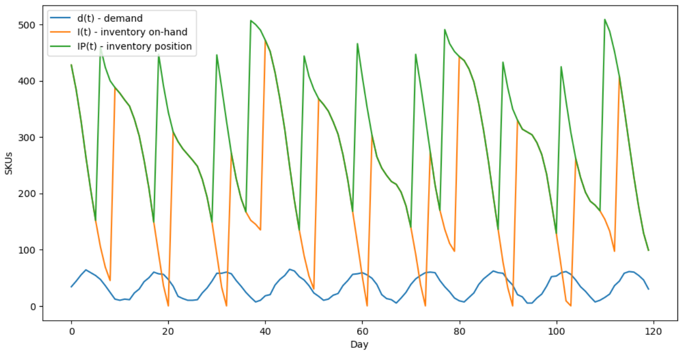
These formulas describe the entire simulation process as well as the parameters required for optimization. To support interpretability, we present the stochastic demand described earlier, along with the operation of the policy and the simulator, using an example. The figure below shows a 120-day demand time series based on an (s, Q) policy. The blue line represents the daily demand, which has a 14-day periodicity. Its value was determined randomly, resulting in the base level (b), the amplitude (A), and the stochastic noise ($\epsilon$). The green line represents the total inventory position (IP), which consists of existing stock and stock awaiting arrival; the orange line represents the currently received and usable stock level. The green and orange lines largely overlap; they diverge when an order is placed due to the nature of the policy, at which point the on-hand stock and total quantity differ until the lead time (L) days when the order arrives. Figure 5 shows that in certain cases, the on-hand stock is smaller than the demand, resulting in a backorder. Based on these parameters, the simulation can calculate the total inventory cost as well as the fill rate.

3.2. Integration of Multiple Inventory Policies

When applying multiple policies, their parameters differ because their meanings and ranges are different. This situation can cause problems during optimization, as it results in a fixed-length vector, and the surrogate model can only operate in a numerical feature space. One of the goals of the developed framework is to be able to handle multiple different policies, which significantly contributes to the realistic application of the system, as strategic decisions in industrial practice also require the application of different policies. We implement the different inventory policies within the framework by introducing a unified representation for the purpose of common optimization.

The framework describes every possible solution in an encoded representation called a candidate. This consists of two parts: a policy identifier (m) and a fixed-length gene vector (g):

$$c=\left(m, g\right),$$

(34)

$$m\in \mathbb{N},$$

(35)

$$g=\left(g_1, g_2,\dots ,g_n\right),$$

(36)

where the following applies to every gene:

$$g_i\in \left[0,1\right], i=1,\dots ,n.$$

(37)

We generate the initial population from various random candidates, which must be decoded. The unified representation values are important for the optimization algorithm and the ML model, while the decoded, real parameters are important for the simulation. Decoding can be formally described as the following mapping:

$$D:\left(m, g, e\right)\mapsto \left(\pi ,\theta \right),$$

(38)

where m is the candidate identifier, g is the gene vector, and e is the vector of environmental statistics. The purpose of this parameter is to allow certain parameters of the inventory simulator to be predefined for population specification in order to ensure realistic modeling. In the framework, we define the average demand and average lead time values:

$$e=\left(d_{mean}, L_{mean}\right),$$

(39)

The result of the decoding is the selected policy ($\pi$) and its parameters ($\theta$). The various policies can be listed in the following set:

$$\Pi =\left({\pi }_0, {\pi }_1, \dots , {\pi }_{M-1}\right),$$

(40)

When generating the population, we map the candidate ID to a valid policy ID using a modulus based on the size of the policy set:

$$m^{\prime }=m mod M,$$

(41)

$$\pi =\Pi \left({\mathrm{m}}^{\prime }\right).$$

(42)

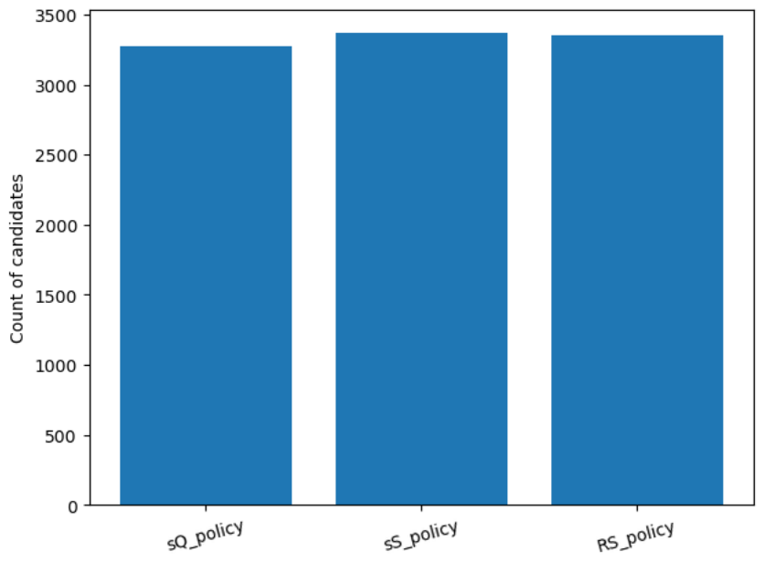
This ensures that each candidate can always be assigned to one of the defined policies, while random sampling guarantees an even distribution across the policies. Figure 6 illustrates the distribution of inventory policies decoded from randomly generated candidate solutions. The results show that the three policy types appear in approximately equal proportions. This confirms that the encoding and decoding processes are unbiased, and that a balanced policy space is created during the optimization process.

The parameters of a policy can be represented by gene vectors. A precondition for this is the definition of the parameters’ bounds. In a stock-based modeling system, it is essential to define the ranges of the various parameters, as this significantly reduces modeling costs and aids in the creation of realistic policies. The set of parameters for a policy can be modeled as follows:

$$P_{\pi }=\left\{p_1, p_2, \dots , p_k\right\},$$

(43)

These intervals depend on the given environmental statistics (e). Therefore, their bounds can also be interpreted in terms of those statistics:

$$p_j=\left[l_j\left(e\right), u_j\left(e\right)\right], j=1,\dots ,k.$$

(44)

For example, in a given environment:

$$s \in \left[0, 100\right],$$

(45)

$$Q\in \left[1, 150\right],$$

(46)

$$S \in \left[1, 200\right],$$

(47)

$$R \in \left[1, 14\right].$$

(48)

When representing genes as real parameters, these limits must be taken into account. This is done by rescaling the gene value (whose range is $g_j\in \left[0, 1\right])$ to fall within the parameter limits, and finally rounding it to the nearest integer:

$${\theta }_j=l_j+g_j\ast \left(u_j-l_j\right),$$

(49)

Parameters are assigned based on their index. Since the policy contains k parameters and the gene vector is n-dimensional, if there are more parameters than dimensions, the gene vector can be used in a circular manner. Otherwise, certain dimensions of the gene vector will not be used.

Finally, policy-specific cases must be handled, as certain policies require the application of logical constraints. A (s, S) policy is only valid if $S\ge s$, since the order level is not greater than the post-order level; therefore, if this condition is not met, the system corrects it: $S≔s$. In the case of the (R, S) policy, both parameters must be positive. Thus, if this condition is not met after decoding, the system must also correct it: $R≔\mathrm{m}\mathrm{a}\mathrm{x}(1,R)$, $S≔\mathrm{m}\mathrm{a}\mathrm{x}(1,S)$.

The output of the decoding process is therefore a specific policy and its parameter vector, which can be used directly in the simulation; the result of this is the f objective vector:

$$D:\left(c, e\right)\mapsto \left(\pi ,\theta \right),$$

(50)

$$\left(\pi ,\theta \right)\mapsto f.$$

(51)

3.3. Multi-Objective Optimization

The second objective of this research is the application of multi-objective optimization. This differs from the general EOQ model, which aims only to achieve minimum cost. In industrial practice, however, numerous other factors are important for a manufacturing company, and the order of priority among these factors depends on the specific strategic decision. When creating a realistic framework, it is essential to consider multiple objectives and apply multi-objective optimization. In the course of the research, we identified three objective parameters, which have already been described in the Research Objectives chapter. In addition to minimizing costs—a factor also present in the classic EOQ model – we defined the maximization of the service level and the minimization of the average inventory level.

As a preparatory step for optimization, it is important to note that the inventory simulator generates parameters suitable for optimization. The following parameters must be specified for the simulation:

-

Time horizon (T);

-

Initial inventory level;

-

Unit ordering cost (K);

-

Unit holding cost (h);

-

Unit shortage cost (p).

The specific parameters generally depend on the industrial partner and can be extended to encompass supply chain-wide optimization. However, this is not the objective of the present study. In addition to initializing the initial parameters, the simulator requires the selected policy and its parameters to be specified. After the preparatory processes, the simulation generates the target values used by the optimization. The goal of the optimization algorithm is to determine a result that meets the various criteria.

After completing the preparatory steps, we perform multi-objective optimization. To achieve this, we use the previously mentioned NSGA-II algorithm, which is one of the most widespread and frequently used multi-objective algorithms. In the research problem, we optimize a nonlinear, simulation-based stochastic system that does not require an analytical model, as the system is not closed-form and has no definable gradient. NSGA-II operates on a population-based principle, so it does not require continuity [31]. Thus, it can handle discrete policies and integer parameters well, and global search is also feasible, since the algorithm does not get stuck in local optima due to the population. The model yields a Pareto front, which is a set of trade-offs containing solutions from which no single best solution can be chosen; rather, each element can be considered the best according to some criterion [32].

The research problem can be interpreted as a multi-objective optimization problem, where the solution is $x\in X$, where x represents the policy parameters:

$$x=\left(x_1, x_2, \dots , x_d\right),$$

(52)

Each solution corresponds to multiple objective function values, and the research problem involves minimizing these values simultaneously:

$$f\left(x\right)=\left(f_1\left(x\right), f_2\left(x\right), \dots , f_m\left(x\right)\right),$$

(53)

$$\underset{x\in X}{\mathit{min}} f\left(x\right),$$

(54)

In this research, therefore, the objective of maximizing inventory levels must be reversed, since the optimization algorithm can handle only one type of optimization; thus, instead of this parameter, the objective is to minimize the fill rate. Consequently, the objective function can be written as follows:

$$f\left(x\right)=\left(total cost, 1-fill rate, average on hand\right).$$

(55)

Given two solutions, solution x dominates solution y if solution x is at least as good as solution y on every objective and better than solution y on at least one objective. This logic helps determine the hierarchy among the solutions:

$$x\prec y, if \forall k:f_k\left(x\right)\le f_k\left(y\right) and \exists k:f_k\left(x\right)<f_k\left(y\right),$$

(56)

The algorithm then sorts all individuals in the population into fronts using the principle of non-dominated sorting. A solution is considered non-dominated if there is no other solution that is better than it in every respect. These can be regarded as compromise solutions, since none is clearly better than the others, but each excels in a particular parameter. These solutions are placed in the first front:

$$F_0=\left\{x\in P \right| \nexists y\in P: y\prec x\}.$$

(57)

The non-dominated solutions can be regarded as the current Pareto front. The second front consists of those individuals that are dominated only by elements of the first front, and this process is repeated. Based on the fronts, each individual is assigned a rank, and the lower the rank, the better the individual is considered to be:

$$rank\left(x\right)=i if x\in F_i,$$

(58)

If two solutions lie on the same front, the algorithm makes a decision based on the crowding distance function. This measures how sparsely or densely a given individual is distributed within the target function space. The algorithm favors the higher value because such individuals better preserve the diversity of the target function set:

$${CD}_i={\displaystyle \sum _{k=1}^m}{\displaystyle \frac{f_k^{i+1}-f_k^{i-1}}{f_k^{max}-f_k^{min}}}.$$

(59)

The selection step can be carried out based on the previously determined rank and crowding distance values. This process is one of the key steps of the algorithm and models natural selection. For two individuals, the one with the lower rank is considered better, or, in the case of equal ranks, the one with the larger crowding distance value. This ensures that the algorithm strives simultaneously for convergence and the preservation of diversity. During selection, the algorithm selects two individuals from the population, and the one with the better value becomes the parent. It repeats this process twice, selecting two better solutions from four. The algorithm then creates new individuals, or offspring, which can also be called child individuals:

$$x^{\left(child\right)}=variation(x^{\left(p1\right)}, x^{\left(p2\right)})$$

(60)

There are three main steps to creating a new individual: first, the child is generated from the parents’ parameters, which serves to pass on the traits of both parents:

$$x_j^{\left(child\right)}=\left\{\begin{array}{c}{x}_j^{\left(p1\right)}\\ x_j^{\left(p2\right)}\end{array}\right.$$

(61)

Next, in the mutation step, the resulting child individual is slightly modified by a random shift ($\Delta j$), which must be normalized to the specified range. The purpose of this is to ensure that the new individuals possess their own characteristics and are not merely combinations of their parents:

$$x_j^{\prime }=x_j+\Delta j$$

(62)

Finally, the algorithm repeats these steps until the number of offspring equals the number of parents. The process of generating offspring ensures the creation of new solutions, their combinations, and their fine-tuning:

$$Q_t=\{x_1^{\left(child\right)}, x_2^{\left(child\right)}, \dots , x_N^{\left(child\right)}\}$$

(63)

After the child population is generated, the algorithm combines it with the original parent population ($P_t$) to create the combined population:

$$R_t=P_t\cup Q_t$$

(64)

The algorithm applies the specified ranking functions to the new population and repeats this process iteratively until the specified number of generations is reached, resulting in the formation of the Pareto front, which contains compromise solutions between the various objective functions.

After initializing the algorithm, we integrate it into the complete framework and perform the optimization on a randomized population. We examine the framework’s performance over a 365-day time horizon, for which we randomly generate a demand time series based on the parameters presented. The selection of this time horizon is justified by the fact that the model’s stable and balanced performance can be clearly observed over a 365-day period, whereas a shorter period does not fully reflect this and may lead to a biased performance evaluation. Furthermore, annual seasonality is commonly observed in many real-world inventory systems, especially in the procurement of raw materials, where demand is influenced by yearly cycles such as market trends, production planning, and external factors.

The optimization always runs on the same demand, so the different simulations are easily comparable. When defining the simulation environment, we specify the initial inventory and the unit costs, which are constant values, and from these, we determine the environmental statistics required for decoding (average inventory level and lead time). We then set the boundaries of the unified search space presented in the previous subsection. Its elements are the candidate identifier, from which the policy can be derived, and the candidate’s gene vector. By applying this, we ensure that every policy appears in the same unified search space; that is, the optimizer does not treat different policies separately but is able to represent every instance using the same structure. The gene values must be normalized to the range [0, 1]:

$$(candidate id,g_0, g_1,g_2)$$

(65)

The step following decoding is simulation, which allows us to define objective functions for the decoded poly and its parameter values, with the goal of minimizing each of them. After this, all prerequisites are in place for the framework to perform the optimization. In the presented example, the NSGA-II algorithm is configured with a population size of 80 and 40 generations, resulting in a total of 80 + 40 ∗ 80 = 3280 simulation evaluations. During the selection of parameters, the main consideration was to efficiently explore the search space while maintaining computational efficiency. Increasing the population or generation size would have resulted in significant computational costs, while we observed that increasing the parameters did not lead to substantial changes in the structure of the resulting Pareto front, which confirms that the selected configuration provides reliable results.

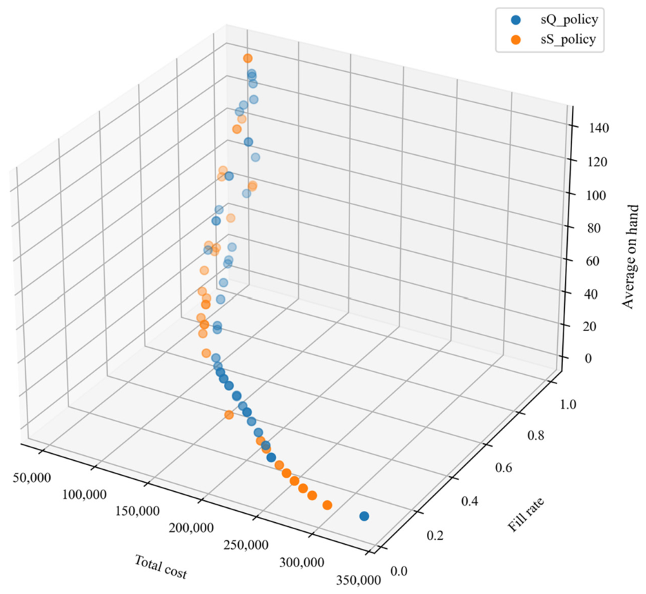
The framework operates successfully; the simulation of the objective functions and the resulting multi-objective optimization were supported by realistic, randomized demand data. During testing of the framework, we initialized numerous parameters with realistic values, and the optimization results are also realistic, making them well-suited for application to real-world industrial data. The result of running the framework is the Pareto front, which can be seen in the figure below. For visualization, we converted the fill rate parameter back to its original, maximized form. Figure 7 shows that none of the possible solutions for the (R, S) policy made it onto the Pareto front.

Based on the examined scenario, the absence of the (R, S) policy can be explained by differences in demand characteristics, cost structures, and operating methods. It is particularly important to note that the (R, S) policy differs significantly from the other two cases, as it is based on periodic analysis, which limits its responsiveness to short-term demand fluctuations in the case of seasonal demand. Consequently, based on the target parameters examined, the following policy is less favorable than the (s, Q) and (s, S) models.

3.4. Application of Surrogate Model

Based on the results presented above, the framework is well-structured and capable of effectively applying multiple policy strategies to a realistic demand time series. The main limitations of the framework are runtime and computational costs, as the NSGA-II algorithm involves many generations of iterations, and simulating inventory levels over these generations is a computationally intensive task. To support this, we defined the third objective of the research: the application of a surrogate model. A surrogate model is a computationally cheap approximation model that emulates the behavior of an expensive simulation model [33]. In this research, we investigate the extent to which simulation costs can be reduced by using a surrogate model and to what extent this degrades the quality of the evaluation.

A surrogate model does not refer to a specific algorithm but rather to a concept aimed at reducing simulation costs and runtime using machine learning-based solutions. The specific solution is generated by a regression model. In this research, we use the Random Forest Regressor model to generate predictions that replace simulations. This algorithm is capable of handling nonlinear relationships well, performs well in noisy environments, and requires little preprocessing [34]. These properties are key to model selection, as the model must handle the nonlinear effects arising from various policy parameters as well as the noisy demand time series.

The selection of the Random Forest regressor is motivated by its robustness and stability in stochastic environments in contrast to more complex models (e.g., neural networks). When choosing the model, these advantages were particularly important, since it is only a small part of the overall framework. Our goal was therefore to select a model that is simple yet highly effective.

To analyze the contribution of the surrogate model, we will examine a specific case. The simulation environment covers a 365-day time horizon. The real simulation and the surrogate model operate on the same seasonal demand pattern, making the results of the two runs easily comparable. We use the same values for the population and generation parameters as in the previous subsection, so the real, simulation-based result is based on a total of 3280 simulations. In addition, we initialize the initial inventory level, the specific order cost (K), holding cost (h), and shortage cost (p). To simplify the comparison process, we apply only the (s, Q) policy, for which we define the value bounds to produce the realistic results mentioned in the previous sections. The simulation results in the real Pareto front, for each element of which ($n_1$) the objective function vector is stored. We organize these into the following matrix:

$$F_{NSGA}\in {\mathbb{R}}^{n_1\ast 3},$$

(66)

We compare these values with the results of simulations supported by the surrogate model. The key point here is that not every candidate solution needs to be evaluated through simulation. Instead, the model uses an approximation algorithm to estimate the target values of certain individuals.

The first steps of the method involve creating an initial training set (300 candidates). The goal is to generate combinations of decision variables. Here, the target value vectors are determined through real simulations. Choosing the right size for the dataset is crucial, as too few samples will result in an inaccurate model, while too many samples render the approach ineffective, since its primary goal is to reduce the need for real simulations.

Next, we fit the previously described regression model to the initial training set, which learns the relationships between the input parameters and the target value vectors. As a result, this model can later be used to approximate the actual simulation. During the execution of the optimization algorithm, the majority of the population is evaluated not by the actual simulation, but by this regression model. During execution, dominance determination, non-dominated sorting, and selection are based on these estimates, thereby achieving faster execution times.

In order to achieve realistic results, the model evaluates a smaller set (20 candidates) in each generation using real simulations; 15 of these candidates are close to the Pareto front, allowing us to assign real simulation values to them, while the purpose of the remaining 5 candidates is to cover new areas in the search space and thereby avoid local optima. The actual evaluated samples are added to the training set, causing this set to grow continuously. We retrain the model iteratively, making it increasingly accurate. The result of the surrogate model-assisted optimization is also the Pareto front, whose elements ($n_2$) are included in the following set:

$$F_{Surr}\in {\mathbb{R}}^{n_2\ast 3}$$

(67)

The sizes of the two sets reflect the extent to which the surrogate model contributed to the optimization:

$${\displaystyle \frac{F_{Surr}}{F_{NSGA}}}={\displaystyle \frac{554}{3280}}\approx {\displaystyle \frac{1}{6}}$$

(68)

Thus, by using the surrogate model, the simulation cost – runtime of the framework—was significantly reduced to one-sixth of the original. This represents a significant speedup, and as a result, the industrial applicability of the framework has increased considerably. However, it is important to examine the extent to which this acceleration is achieved at the expense of optimization results. First, we examine the extent to which the best elements of the three objective values have changed. The results are shown in

Table 2. Comparison of model results (source: Python).

	Cost	Fill Rate	Average Inventory Level
NSGA-II	40,954	1	1.02
Surrogate-assisted model	43,699	1	1.02
	107%	100%	100%

.

An analysis of each parameter individually shows that surrogate-assisted optimization did not achieve the same best result for cost minimization alone as it did for the other two parameters. This can be considered a particularly good result; however, more advanced methods can also be used for a constructive comparison of multi-objective optimization models. Hypervolume (HV) measures the volume of solutions defined by the Pareto front relative to a predefined reference point. Its value reflects the model’s convergence, i.e., the proximity of the solutions to the optimal point; diversity, which indicates the degree to which solutions are scattered along the front; as well as the coverage of the front. Thus, HV is a complex metric that effectively reflects the accuracy and distribution of solutions. When comparing the results of different methods, a higher HV value is considered to indicate better performance [35].

The HV value of the model based on full simulation is 1.168, while that of the surrogate-assisted optimization model is 1.123. In terms of the HV parameter, the original model performs 4% better. To summarize the results of the surrogate model, the runtime of the accelerated model is nearly one-sixth that of the original, full simulation model, while its performance is only 4% better. This improvement in runtime is a drastic and significant result for the operation of the entire framework, while its performance has deteriorated only minimally. Based on these values, it can be concluded that the implementation of the surrogate model into the framework is successful and useful.

To evaluate the accuracy of the surrogate model, we computed standard regression error metrics, including Mean Absolute Error (MAE), Root Mean Squared Error (RMSE) normalized RMSE (NRMSE), and the coefficient of determination (R²), for each objective function. The results indicate that the surrogate model provides sufficiently accurate approximation across all objectives. The R² are consistently high (above 0.97), which demonstrates and excellent fit between predicted and true values. Although the prediction error is higher for the inventory level, this can be attributed to the increased variability of this objective in stochastic inventory systems. The reported metrics are computed on candidate solutions that were re-evaluated by the true simulator during the refinement phase of the surrogate-assisted optimization (

Table 3. Prediction accuracy of the surrogate model (source: Python).

	Cost	1-Fill Rate	Average Inventory Level
MAE	6283	0.02	1.45
RMSE	31,288	0.05	4.77
NRMSE	11%	11%	17%
R2	0.98	0.97	0.97

). In summary, the total error remains within an acceptable range for surrogate-based optimization, while the runtime is reduced to approximately one-sixth of the original.

Following the initial implementation and experimental results, we tested the presented model using various parameters to examine the variability arising from stochastic demand modeling and the random behavior of the algorithm. We performed a total of 25 runs, based on five different demand scenarios and seed combinations. Based on the results, the surrogate-based approach resulted in an average 3.1% reduction in HV compared to the standard NSGA-II algorithm, while the number of simulation evaluations decreased by an average of 5.39 times. The results of the more robust evaluation differ minimally from those of the initially implemented model, but their scale is the same, thereby further validating the research findings.

To evaluate the unified approach we developed, we used the same 25 runs employed for the robustness evaluation to compare it with a single policy-based benchmark, in which we optimized each inventory strategy separately using the NSGA-II algorithm, and then subsequently unified the resulting Pareto fronts and selected the best solution set. The results show that the average HV value of the developed unified framework (without surrogate assistance) is 1.134, while the average HV value of the benchmark single-policy method is 1.144. There is a total difference of only 0.9% between the two values, which is practically negligible. It is important to note that the single-policy method requires three different optimizations, resulting in significantly longer runtime despite minimal improvement. Since examining implementation time was among the research objectives, the developed framework is a significantly more favorable solution due to automatic policy selection, as it provides a more flexible and efficient solution in practical applications (

Table 4. Aggregated results across multiple demand scenarios and random seeds (source: Python).

Method	n	HV (Mean, Std)	95% CI	Best Cost (Mean, Std)	Evaluations (Mean)	Pareto Size (Mean)
Surrogate NSGA-II	25	1.099 ± 0.062	±0.024	47,278 ± 13,034	611	80
Unified NSGA-II	25	1.134 ± 0.055	±0.021	44,976 ± 11,750	3280 ± 0	80
Single-policy NSGA-II	25	1.144 ± 0.052	±0.020	44,884 ± 11,774	9840	132

).

We conducted our research using a randomized, noise-contaminated demand time series, in which the initialization parameters were also randomly selected; thus, a potential avenue for further research is the extension of the framework to real-world industrial problems. On the one hand, this can provide feedback on the level of applicability resulting from the research contributions; on the other hand, practical cases can define new simulation tasks.

4. Discussion

During the research, we formulated three objectives, which were successfully applied and implemented. The main contribution of the research was the creation of a realistic framework for inventory modeling, based on the classic EOQ model and utilizing its various policy strategies.

The first research question examined the integration of different policies. The aim was to define the various strategies within a common optimization space. The methodology developed made it possible to handle inventory models based on different operational strategies within a common search space, thereby making them directly comparable—a significant advantage in an optimization problem. The results showed that multiple policy settings can be found on the Pareto front, so a relational connection cannot necessarily be established between policy types, as their settings are crucial during optimization. This extension of the search space significantly improves upon traditional inventory models, as in general modeling, the policy strategy is a preliminary decision, whereas in our research, it has become part of the optimization process.

During the selection of algorithm parameters, our primary goal was to strike a balance between computational cost and stable convergence. In the case of NSGA-II, the population size and number of generations were chosen to ensure adequate diversity, thereby enabling simulation-based evaluation. For the surrogate-assisted model, when selecting parameters, we ensured that the model could maintain predictive accuracy while reducing computation time. The Random Forest model and its parameters are designed to deliver stable performance on the nonlinear problem, thereby fitting well within the established framework.

To assess robustness and reliability, we conducted several demand scenarios using different random seeds. Furthermore, we evaluated predictive accuracy using the MAE, RMSE, NRMSE, and R² metrics. These provided statistical validation of the quality of the optimization and the reliability of the surrogate-assisted method. The results of repeated runs confirmed that the developed framework is capable of reaching the optima on the Pareto front with significant reductions in computational cost.

NSGA-III is indeed a more advanced and modern algorithm. However, the goal of this research was to select an algorithm that is truly reliable and has been validated in numerous academic publications. As a result, NSGA-II proved to be the appropriate choice due to its simplicity and robustness. The primary goal of the research was to create a framework in which the optimization algorithm is one of the building blocks; therefore, the main focus was on creating a unified framework. At the same time, the application of NSGA-III could be an important future research direction for creating an up-to-date and advanced framework.

The application of multi-objective optimization is particularly important when creating a realistic inventory model, and it goes significantly beyond the models used to date. The result of the optimization is the Pareto front, which presents a set of optimal solutions from which no single best solution can be selected, as this depends on the specific industrial situation.

Simulating various scenarios is essential for population-based optimization algorithms. This method involves significant simulation costs, as the algorithm operates iteratively and requires a large number of simulations even within a single iteration. The integration of the surrogate model significantly reduced simulation costs, thereby increasing the computational efficiency of the entire framework. The model, which functions as a regression approach, was able to preserve the quality of the Pareto front while significantly reducing simulation costs. The trade-off is negligible compared to the simulation improvement, and its use clearly demonstrates the level of contribution that state-of-the-art ML-based methods can provide to simulation-based optimization procedures.

The proposed framework provides a practical decision-support tool for inventory optimization. Instead of focusing on a single optimization objective, the framework offers a set of solutions for the simultaneous optimization of multiple practical objectives, enabling industrial managers to select the solution that best aligns with their strategic goals from among several optimal solutions during practical application. Furthermore, it is not necessary to pre-select an inventory optimization strategy, as the framework is capable of managing and specifying multiple policies. These practical capabilities contribute significantly to agile, simulation-based decision assistance.

5. Conclusions

The aim of the research was to develop a realistic inventory modeling framework. As a first step, we described its relationship to Lean and JIT, as well as the findings and distribution of the published literature. Regarding previous research, it can be concluded that most studies are primarily academic in nature, and numerous further developments are required for their application in industrial practice. To achieve this goal, the research defined three objectives.

By unifying the various inventory strategies, we have ensured that strategy selection is not a preliminary decision-making step but rather is integrated into the optimization process and becomes part of it. As a result, the set of final results includes solutions for multiple policies. Classic EOQ solutions aim to minimize costs; however, in logistics inventory optimization, objectives cannot be limited to this alone, so we expanded the objectives and created a framework for multi-objective optimization. In addition to minimizing costs, we defined the objectives of maximizing demand fulfillment and minimizing average remaining inventory. To implement the optimization, we applied the NSGA-II algorithm, which was capable of determining the optimal Pareto front. During the execution of the simulation-based framework, it was observed that simulation costs are significant in the system. To address this, we employed a surrogate model, which significantly reduced the framework’s runtime with minimal compromise. Its application represents a significant scientific contribution to this problem and, more generally, to the use of ML methods in optimization problems.

The research focused on establishing a framework, which has made it possible to identify a number of limitations and opportunities for further development. The experiments are based on synthetically generated demand data with a fixed seasonal structure, and the validation is limited to a specific set of parameter configurations. In addition, the surrogate model introduces approximation errors, which, although controlled, may affect the accuracy of the optimization results in certain cases. Further development can be achieved in several directions. Extending the model to real-world industrial data could open up new modeling possibilities, and the model can also be fine-tuned by analyzing more detailed or complex seasonal trends. Finally, the complete research results could be integrated into the digital twin or smart manufacturing concept, the exploration and integration of which could offer new research opportunities.