Article

Hidden Drivers in Ecological Networks: Detecting Possible Latent Forcing from Time-Series Data

1
College of Information Science and Engineering, Zaozhuang University, Zaozhuang 277100, China
2
College of Information Science and Engineering, Shandong Agricultural University, Taian 271018, China
*
Author to whom correspondence should be addressed.
Algorithms 2026, 19(4), 307; https://doi.org/10.3390/a19040307
Submission received: 12 February 2026 / Revised: 8 April 2026 / Accepted: 9 April 2026 / Published: 14 April 2026

Abstract

Ecological interaction networks are often influenced by unobserved upstream forcing, which can make an observed link between two variables appear causal even when it primarily reflects mediation within a deeper causal chain. This challenges the interpretation of trophic control, the identification of dominant ecological drivers, and the design of effective monitoring strategies. Here, we introduce detecting pairwise effect (DPE), a data-driven method based on empirical dynamic modeling and multivariable state-space reconstruction, to assess whether an observed directional link is more consistent with a direct ecological driver or with a mediated effect shaped by latent upstream forcing. Using benchmark dynamical system motifs, we show that DPE can identify conditions under which a strong upstream driver acting on the putative cause may distort pairwise causal interpretation. We further demonstrate its ecological relevance using real-world time series, where DPE reveals diagnostic signals consistent with hidden trophic forcing in a plankton food-chain dataset and possible latent external forcing in soil-temperature depth dynamics. Overall, DPE provides a diagnostic signal that is consistent with the presence of latent upstream influence, thereby improving the interpretability of inferred ecological causal relationships.

1. Introduction

Ecological interaction networks are shaped by coupled biotic and abiotic processes acting across space and time. In practice, however, ecological monitoring is inevitably incomplete: key environmental drivers, missing taxa, or unrecorded management actions can act as unobserved upstream forcing, leaving only partial time-series observations of the system. This creates a recurrent inferential challenge: an apparent causal relationship between two measured variables may be interpreted as a direct ecological driver, even when it largely reflects mediation within a deeper causal chain [1]. Such ambiguity can limit our ability to interpret trophic control, identify dominant ecological drivers, and design effective monitoring strategies.
To interrogate dynamic interactions from time series, ecologists have increasingly adopted causality inference tools [2]. These include Granger causality [3,4,5], dynamical Bayesian inference [6,7,8,9,10,11], convergent cross mapping (CCM) and related empirical dynamic modeling (EDM) approaches [12,13,14,15,16,17,18], as well as neural network-based methods [19]. These methods have proven valuable for detecting directional dependencies and information flow among observed variables. Nevertheless, real-world ecosystems are inherently complex [20,21,22,23,24], typically comprising large networks of interacting components, and many relevant drivers may remain unknown, unmeasured, or difficult to observe. As a result, existing approaches—largely focused on relationships among measured variables—often provide limited guidance on a critical ecological question: when an observable directional link X → Y is detected, does X represent a direct driver of Y, or is the link primarily a mediated effect shaped by unobserved upstream forcing? If the latter holds, interventions or monitoring centered on X may target a mediator rather than the more proximal leverage point, and mechanistic interpretation of the inferred network can be misleading.
Addressing this gap requires diagnostic tools that can extract evidence of latent upstream structure using only the available time series. To our knowledge, systematically detecting latent causation solely from observable time series in dynamical ecological systems has not yet been fully explored [25,26,27]. In this paper, we propose a data-driven method termed detecting pairwise effect (DPE) to infer latent upstream forcing from two interconnected time series X and Y when an observable directional relationship X → Y has been established. The central idea of DPE is to detect a characteristic signature—termed the pairwise effect—that indicates the observed link X → Y is unlikely to be directly fundamental, but instead embeds a deeper latent chain Z → X → Y, in which X primarily acts as a mediator rather than the root cause of Y.
We validate DPE in simulated benchmark ecosystem motifs with controlled causal structures and then demonstrate its ecological relevance using real-world time series networks. Under appropriate conditions, DPE provides additional insight into whether an inferred link is more consistent with a direct driver or a mediated relationship shaped by latent forcing. By providing an interpretable screening step prior to targeted data collection, DPE complements existing causality inference methods and helps improve the interpretability of causal relationships in complex ecological networks.
The contribution of this study is threefold. First, we propose DPE as a diagnostic framework for assessing whether an observed directional link is more consistent with a direct driver or with a mediated effect shaped by latent upstream forcing. Second, we provide a mechanistic interpretation of how the pairwise effect can arise in systems with hidden upstream structures. Third, we evaluate the method using benchmark dynamical systems and representative ecological and environmental time-series datasets.

2. Materials and Methods

2.1. Detecting Pairwise Effect

Convergent cross mapping (CCM) is a widely used method for causal inference in ecological systems [12]. Based on Takens’ embedding theorem [28], CCM reconstructs shadow manifolds from time series data and exploits nearest-neighbor relationships in the reconstructed state-space to assess causality via predictive skill  ρ [29]. The key idea is that if X causally influences Y (i.e., X → Y), then information about X is embedded in the time series of Y [12]. Consequently, the effect variable can be used to predict the cause. For a pair of time series X and Y, if Y exhibits high predictive skill in reconstructing X, that is, the predicted series  X ^ M Y  closely matches the observed X, this indicates causality in the direction X → Y.
In the original CCM formulation, only the time series of Y is used to reconstruct the shadow manifold  M Y . In addition, it has been shown that a time series can accurately predict itself, yielding a high self-prediction skill  ρ ( Y , Y ^ | M Y )  that typically approaches 1 [30] (see Section 2.3 for details). A similar property holds for  ρ ( X , X ^ | M X ) .
In this study, we propose a data-driven method termed detecting pairwise effect (DPE), which extends CCM by introducing multivariable embedding [29,31,32] into the reconstruction process. Specifically, when reconstructing the manifold of Y, we incorporate not only Y itself but also information from X, resulting in a multivariate shadow manifold  M Y , X . When predicting Y based on  M Y , X , the inclusion of X may act as an additional perturbation, reducing the purity of the reconstructed manifold. As a result, the predictive skill typically decreases, i.e.,
ρ Y , Y ^ M Y , X < ρ Y , Y ^ M Y
In a simple dynamical system involving two variables X and Y, if there exists a unidirectional causal relationship X → Y, then Y, as the effect, contains information about X, whereas X, as the cause, contains limited information about Y. Consequently, under multivariable embedding, we expect:
ρ X , X ^ M X , Y > ρ Y , Y ^ M Y , X
However, real-world dynamical systems are typically more complex and often involve additional latent variables beyond X and Y, which we collectively denote as Z. In the DPE framework, these variables may be unobserved or entirely unknown. If the underlying causal structure includes a chain Z → X → Y, then the reconstruction of X from Y can be substantially affected by the upstream influence Z → X. As the strength of this causal link increases, the predictive skill  ρ ( X , X ^ M X , Y )  may decrease significantly. We hypothesize that when the influence of Z → X exceeds a certain threshold, the inequality may reverse, leading to:
ρ X , X ^ M X , Y < ρ Y , Y ^ M Y , X
We refer to this counterintuitive phenomenon as the pairwise effect.
In summary, the central idea of DPE is to compare the predictive skills  ρ X , X ^ M X , Y  and  ρ Y , Y ^ M Y , X . Under an approximately unidirectional causal relationship X → Y, the occurrence of  ρ X , X ^ M X , Y < ρ Y , Y ^ M Y , X  indicates the presence of the pairwise effect. This, in turn, suggests the existence of a deeper causal structure (e.g., Z → X → Y), in which X functions primarily as a mediator rather than the more proximal causal driver of Y.

2.2. Normal Reconstruction

In CCM theory, given a pair of time series X and Y, if Y has a high forecasting skill for predicting X, this indicates a causal relationship in the direction of X → Y. In the original CCM framework, the time series of Y is used to reconstruct the shadow manifold  M Y . The parameter of embedding dimension can be computationally determined by the simplex projection method [31,33]. Given an embedding dimension  E , the reconstructed manifold  M Y  consists of a series of  E -dimensional state vectors  Y t , where each state vector is defined as:
Y t = y t , y t 1 , , y t E 1
The time delay  τ  is fixed to 1 in this study for all experiments unless otherwise specified. Thus, the reconstructed shadow manifold is written as
M Y = { Y t }
The manifold  M Y  can be used to predict the historical data of X. Specifically, the prediction of  x t  at time  t  based  M Y  is denoted as  x t ^ | M Y . To estimate  x t  from  M Y , we first identify the  E + 1  nearest neighbors of the target point  Y t , corresponding to time indices  t 1 , , t E + 1 . Let  d i  denote the Euclidean distance between target point and its  i -th nearest neighbor, and let
d m i n = min j   d j
be the minimum of these distances. Euclidean distance is used to identify nearest neighbors in all embeddings. The weight assigned to the  i -th neighbor is defined as:
W ( i ) = e x p ( d i / d m i n ) j = 1 E + 1 e x p ( d j / d m i n )
Accordingly, the prediction of  x t  based on  M Y  is given by:
x t ^ | M y = i = 1 E + 1 W i x t ( i )
The predictive skill of CCM, denoted as  ρ ( X , X ^ | M y ) , can be quantified by the Pearson correlation coefficient between real  X  and predicted  X ^ . If the causal direction is X → Y, the  ρ ( X , X ^ | M y )  will generally increase and eventually converge to a numerical value as the library length  L  increases, although there may be small fluctuations in the numerical value. In this study, we use the value obtained at the largest library length  L  as the predictive skill. By contrast, under unidirectional causality,  Y  cannot be reconstructed from the time series of  X  with comparable accuracy, and therefore:
ρ Y , Y ^ M X < ρ X , X ^ M Y .

2.3. Computing Process

As indicated by previous research [30], the time series of Y can also be used to predict itself, typically yielding a very high predictive skill, denoted by  ρ ( Y , Y ^ | M Y ) . Similarly, the time series of  X  can be used to predict itself, with predictive skill denoted by  ρ ( X , X ^ | M X ) . In the DPE method, multivariable embedding [31] is introduced into the reconstruction of the shadow manifold. Specifically, when reconstructing the manifold of Y, we incorporate information from  X  into the state vector. The simplest multivariable state vector is defined as:
( Y ,   X ) t = y t , y t 1 , , y t E 1 , x t
The corresponding multivariate shadow manifold is denoted by:
M Y ,   X = { ( Y ,   X ) t }
More generally, the form of multivariable embedding is not unique. For example,  x t , y t , y t 1 , , y t E 1  and  y t , y t 1 , , y t E 1 , x t , x t 1  are also valid alternatives. In this study, we use the form given in Equation (5) for consistency and clarity. This is chosen as the simplest extension of the univariate embedding, incorporating only the contemporaneous value of the additional variable to avoid unnecessary increases in dimensionality and potential overfitting.
Prior to embedding, all time series are normalized to zero mean and unit variance. This ensures that variables with different scales contribute comparably to the Euclidean distance calculation and prevents any single variable from dominating the nearest-neighbor search and weight assignment.
Using  M Y , X , the predictive skill for reconstructing  Y  is quantified by the Pearson correlation coefficient between the observed series  Y  and the predicted series  Y ^ M Y , X , denoted by  ρ Y , Y ^ M Y , X . In this paper, the predictive skill  ρ  is defined as the Pearson correlation coefficient between the observed series and the predicted series obtained via cross mapping. Predictions are generated using a leave-one-out strategy, where the target point is excluded from the library when identifying nearest neighbors, ensuring that the prediction is out-of-sample. The predictive skill is evaluated as a function of library size  L , and the value at the largest  L  is used for comparison.
Because the introduced variable  x t  does not directly improve self-reconstruction of  Y  in the pairwise setting and may act as an additional perturbation, we typically observe
ρ Y , Y ^ M Y , X < ρ Y , Y ^ M Y
Similarly, when reconstructing the manifold of X with the aid of Y, we define:
( X ,   Y ) t = x t , x t 1 , , x t E 1 , y t
with the corresponding multivariate shadow manifold:
M X ,   Y = { ( X ,   Y ) t }
The associated predictive skill is denoted by  ρ X , X ^ M X , Y .
For a dynamical system with two observed variables X and Y, if there is a unidirectional causal relationship X → Y, then Y contains information about X, whereas X does not contain comparable information about Y. Consequently, under multivariable embedding, we expect:
ρ X , X ^ M X , Y > ρ Y , Y ^ M Y , X
However, real dynamical systems are usually more complex and often involve additional latent variables beyond X and Y. In this paper, such latent variables are collectively denoted by Z. If the true causal structure contains a latent upstream chain Z → X → Y, then the ability to reconstruct X from information contained in Y may be substantially affected by the hidden driver Z. In particular, as the causal strength of Z → X increases, the predictive skill  ρ X , X ^ M X , Y  may decrease markedly.
Importantly, the presence of Z does not invalidate the conventional CCM inference for the observed pair X → Y. That is, standard CCM can still correctly indicate the directional asymmetry:
ρ Y , Y ^ M x < ρ X , X ^ M y
Nevertheless, when the causal effect of Z → X is sufficiently strong, the multivariable embedding comparison may yield:
ρ X , X ^ M X , Y < ρ Y , Y ^ M Y , X
which appears counterintuitive under the simple pairwise interpretation. In this paper, we refer to this phenomenon as the pairwise effect.
In addition, if the latent variable Z also exerts a strong influence on Y (i.e., Z → Y), then  ρ Y , Y ^ M Y , X  may also be substantially affected, in which case the pairwise effect may weaken or even disappear. Therefore, when analyzing a pair of observed variables, the presence of the pairwise effect suggests that unobserved factors in the system exert a strong influence on X while having limited influence on Y.
For convenience, we define the DPE contrast as
Δ D P E = ρ X , X ^ M X , Y ρ Y , Y ^ M Y , X
Under ordinary pairwise causality X → Y, we expect  Δ D P E > 0 . When a strong latent upstream driver affects X,  Δ D P E  will become negative  Δ D P E < 0 , indicating the occurrence of the pairwise effect.

2.4. Mechanistic Interpretation

To better understand the mechanism underlying the pairwise effect, we provide a conceptual and analytical explanation of how an upstream latent driver alters the asymmetry of predictive skill in multivariable embeddings.
Unlike conventional machine learning frameworks, CCM does not employ an explicit train/test split or rolling validation. Instead, predictive performance is evaluated within the library-based framework, where predictions are generated using nearest neighbors selected from a library of size L. By progressively increasing L, the convergence of predictive skill reflects the strength of the underlying causal signal.
In CCM, the ability to reconstruct a variable from another relies on the extent to which information about the former is redundantly encoded in the latter through the underlying dynamical system. When a causal relationship X → Y exists, the dynamics of Y are partially driven by X, and therefore the reconstructed manifold  M Y  contains information about X. This redundancy enables accurate recovery of X from Y-based embeddings.
However, consider a system in which an additional latent variable Z influences X but has little or no direct effect on Y, forming a causal chain Z → X → Y. In this case, the variability of X can be decomposed into two components: (i) the portion transmitted to  Y  through the link X → Y, and (ii) the portion induced by Z that is not fully propagated to Y. As the strength of Z → X increases, a larger fraction of the variation in X originates from Z, while only a limited part of this variation is reflected in Y. Consequently, the redundancy of information about X in the reconstructed manifold  M Y  is reduced.
Under multivariable embedding, when constructing  M X , Y  and  M Y , X , this asymmetry becomes more pronounced. The reconstruction of X from  M X , Y  relies on the information about X that can be inferred from Y. When the influence of Z is strong, the component of X driven by Z is not sufficiently encoded in Y, leading to a degradation in predictive skill  ρ ( X , X ^ M X , Y ) . In contrast, the reconstruction of Y from  M Y , X  is less affected, since Y remains primarily driven by X, and the additional variability introduced by Z does not directly disrupt the mapping from X to Y. As a result, the inequality  ρ X , X ^ M X , Y > ρ Y , Y ^ M Y , X  may be weakened and eventually reversed as the strength of Z → X, giving rise to the pairwise effect.
To further illustrate this mechanism, consider a simplified linear dynamical system:
X t = a X t 1 + b Z t 1 + ε t , Y t = c Y t 1 + d X t 1 + η t ,
where Z is an exogenous latent driver, and  ε t , η t  are noise terms. In this system, X is influenced by both its own past and the upstream variable Z, while Y is driven by X.
When  b  is small, most of the variability in X is inherited from its own dynamics and is partially transmitted to Y through the coefficient  d . In this case, Y retains substantial information about X, and the predictive skill  ρ ( X , X ^ M X , Y )  remains high.
As  b  increases, a larger portion of the variability in X is driven by Z. If the influence of Z is not proportionally transmitted to Y, the component of X that originates from Z becomes increasingly unpredictable from Y. This reduces the effective information overlap between X and Y, leading to a decline in  ρ ( X , X ^ M X , Y ) . In contrast, the prediction of Y from  M Y , X  remains relatively stable, as Y continues to depend directly on X.
Therefore, when the contribution of Z to the variance of X exceeds that of the transmitted component through X → Y, the inequality between predictive skills may reverse, yielding
ρ ( X , X ^ M X , Y ) < ρ ( Y , Y ^ M Y , X ) .
This provides a mechanistic explanation for the emergence of the pairwise effect in systems with latent upstream drivers.

2.5. Uncertainty Quantification

To quantify uncertainty in the DPE contrast, we define
Δ D P E = ρ ( X , X ^ M X , Y ) ρ ( Y , Y ^ M Y , X ) .
For each simulation and empirical analysis, uncertainty is assessed using a block bootstrap procedure to preserve temporal dependence in the observed series. Specifically, the original time series are resampled using contiguous blocks of length  b , and each bootstrap replicate is used to recompute the predictive skills  ρ ( X , X ^ M X , Y ) ρ ( Y , Y ^ M Y , X ) , and the resulting  Δ D P E . We use  B = 1000  bootstrap replicates in all analyses. The 95% confidence interval of  Δ D P E  is estimated using the percentile bootstrap. A pairwise effect is considered statistically supported when the upper bound of the 95% confidence interval is below zero; if the interval overlaps zero, the result is interpreted as inconclusive rather than as a binary decision. A one-sided bootstrap p-value is computed as the proportion of bootstrap replicates with  Δ D P E 0 .

3. Results

3.1. Detect Latent Causation in Benchmark System

We first use the following simulated benchmark system of three interacting variables to validate our DPE method, as shown in Equation (6). Different values of the coupling parameters  β x y β x z β y x β y z β z x , and  β z y  can lead to various interacting modes and dynamic systems. Although this dynamic system includes the time series of X, Y and Z, only X and Y are involved in the causality detection computation. Z is considered unobservable and therefore excluded from the inference process, limited to result validation.
x t = x t 1 3.60 3.6 0 x t 1 β x y y t 1 β x z z t 1 y t = y t 1 3.72 3.72 y t 1 β y x x t 1 β y z z t 1 z t = z t 1 3.68 3.68 z t 1 β z x x t 1 β z y y t 1
We formulated seven different causal network structures (Figure 1) based on Equation (6), encompassing various basic causal scenarios among three variables. Among these scenarios, a unidirectional strong causal relation X → Y ( β y x  = 0.35) is fixed. The reconstruction parameters in manifold reconstruction for this benchmark system are E = 3, τ = 1 and L = 1500, aligning with common practices in empirical dynamic modeling analysis [34].
The experimental results are shown in Table 1. It can be seen that the DPE method successfully detects pairwise-effect signals consistent with latent external influence (i.e., Z) based on pairwise effect, using only the data from X and Y. Noticeably, the pairwise effect is observed when the latent external variable Z significantly influences X (as observed in scenarios B and E in Figure 1) in the X → Y direction. Specifically, in scenarios where the external factor Z has no impact on either X or Y,  ρ X , X ^ M x + y  is higher (as observed in scenario A), indicating the absence of the pairwise effect. Conversely, in cases where the external variable Z strongly influences X while having weak impact on Y,  ρ Y , Y ^ M y + x  is higher, leading to the presence of pairwise effect (as observed in scenarios B and E). However, when Z had strong effects on both X and Y, the pairwise effect is absent (as observed in scenario D). Moreover, when the influence of Z on X was weak, regardless of Z’s impact on Y, the pairwise effect was always absent (as observed in scenarios C, F, and G).
Here, the DPE interpretation is based on the sign of  Δ D P E  together with its bootstrap confidence interval. A pairwise effect is considered statistically supported only when the 95% confidence interval of  Δ D P E  lies entirely below zero; otherwise, the result is treated as no supported pairwise effect or as inconclusive. We validated our proposed hypothesis in the aforementioned benchmark system, where the pairwise effect only appears in specific causal modes. To further investigate the application of DPE in complex scenarios, we conducted a sensitivity analysis on the strength of causal links.
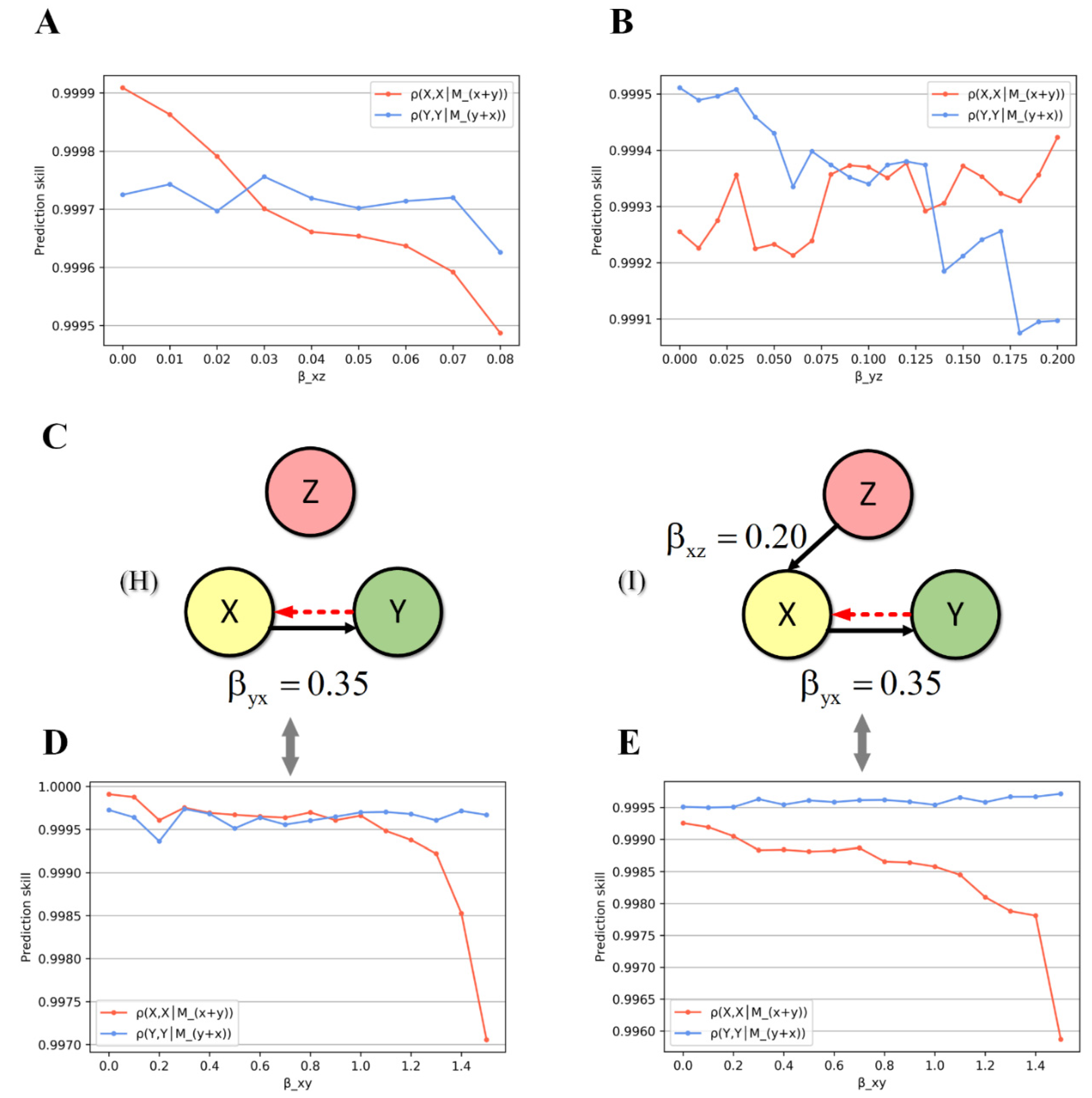
Firstly, we studied the causal chain Z → X → Y, as depicted in scenarios B and C. We maintained  β y x  fixed at 0.35 and incrementally increased the value of  β x z , reflecting the causal strength in the Z → X direction, to observe the emergence of the pairwise effect. The experimental results are presented in Figure 2A. In the figure, when the value of the blue curve surpasses that of the red curve, it indicates the presence of pairwise effect. As observed from the figure, as the causal strength  β x z  in the Z → X direction increases, the red curve representing  ρ X , X ^ M x + y  demonstrates a significant downward trend. This decline implies a reduction in the information on X contained within Y. This reduction occurs due to the growing causal strength of Z → X, which may disrupt the information prediction in X → Y direction. Moreover, the blue curve representing  Y , Y ^ M y + x  remains basically stable. This stability is attributed to the fact that X, as the cause of Y, inherently contained minimal information about Y, which is the consequence of X. Thus, the prediction process remains less affected by the Z → X causal chain link. To conclude, when  β x z  is relatively low, the pairwise effect is not observed. However, as  β x z  gradually increases and surpasses a certain threshold (in this case, 0.025 in Figure 2A), the pairwise effect becomes apparent. The experimental findings aligned consistently with the theoretical analysis.
To quantify uncertainty in the DPE contrast, we further estimated 95% bootstrap confidence intervals for  Δ D P E  in each benchmark scenario (Table 1). The results show that scenarios B and E yield negative  Δ D P E  values, and in both cases the corresponding 95% confidence intervals lie entirely below zero, providing statistical support for the presence of the pairwise effect. By contrast, in scenarios A, C, D, F, and G,  Δ D P E  remains positive and the corresponding confidence intervals remain above zero, indicating no supported pairwise effect under the current decision criterion. These results strengthen the interpretation that the pairwise effect emerges only under specific latent-causal configurations, rather than as a generic consequence of multivariable embedding. Therefore, the benchmark results support the proposed hypothesis that the pairwise effect is selectively induced when the latent upstream variable exerts a sufficiently strong influence on X while having limited influence on Y.
Secondly, we studied the causal network of Z → X → Y and Z → Y as represented by scenarios D and E, with fixed  β y x  at 0.35 and  β x z  at 0.20. We systematically adjusted the value of  β y z , reflecting the causal strength in the Z → Y direction. This continuous adjustment allowed us to observe whether the pairwise effect emerged in the results (Figure 2B). It is evident that when  β y z  was relatively low, indicating a weak causal strength in the Z → Y direction, the pairwise effect became evident. However, as  β y z  progressively increased, the pairwise effect progressively disappeared. In a comprehensive perspective, the blue curve, representing  Y , Y ^ M y + x , displayed a descending trend, while the red curve, representing  ρ X , X ^ M x + y , exhibited an ascending trend. This transition of the pairwise effect from presence to absence underscores that when Z exerts a strong causal influence on both X and Y simultaneously, acting as a confounder in the causal link X → Y, the pairwise effect cannot be observed.
To evaluate the robustness of DPE under realistic data conditions, we conducted a simple stress-test analysis using two representative benchmark scenarios. Scenario A represents a case without latent upstream forcing and is therefore expected not to exhibit the pairwise effect, whereas Scenario B represents a case with a latent upstream chain Z → X → Y and is expected to exhibit the pairwise effect.
For each scenario, we generated simulated time series using the same benchmark system described in Equation (6). We then examined two factors that commonly affect real-world time series analysis: observation noise and time-series length.
For the noise experiment, Gaussian observation noise was added to X and Y:
X t o b s = X t + σ ϵ t , Y t o b s = Y t + σ η t
where  ϵ t  and  η t  are independent standard normal variables and  σ  denotes the noise level. We considered  σ  = 0, 0.01, 0.05, and 0.10. For the sample-length experiment, the DPE analysis was repeated using truncated series with library lengths L = 1500, 1000, 500, and 250.
For each setting, we computed the DPE contrast  Δ D P E , its 95% bootstrap confidence interval, and the corresponding decision outcome. A pairwise effect was considered statistically supported when the 95% confidence interval of  Δ D P E  lay entirely below zero.
As shown in Table 2, DPE remained informative under low to moderate observation noise. In Scenario A, which does not contain latent upstream forcing,  Δ D P E  remained positive across all noise settings, indicating no supported pairwise effect. However, as the noise level increased, the absolute magnitude of  Δ D P E  decreased and the corresponding confidence intervals became wider, reflecting reduced statistical stability. At the highest noise level ( σ = 0.10 ), the confidence interval overlapped zero, and the result therefore became inconclusive. In Scenario B, which contains the latent upstream chain  Z X Y Δ D P E  remained negative under low to moderate noise levels, and the corresponding confidence intervals lay entirely below zero, providing statistical support for the pairwise effect. When the noise level increased to  σ = 0.10 , the confidence interval also overlapped zero, indicating that the result became inconclusive under strong observational perturbation.
A similar pattern was observed for reduced time-series length (Table 3). In Scenario A,  Δ D P E  remained positive for  L = 1500 1000 , and  500 , suggesting no supported pairwise effect, but the result became inconclusive when the available series was shortened to  L = 250 . In Scenario B,  Δ D P E  remained negative and statistically supported for  L = 1500 1000 , and  500 , whereas the confidence interval overlapped zero at  L = 250 , again indicating an inconclusive result. These results suggest that DPE can remain informative under moderate reductions in sample length, but its reliability declines when the available time series becomes too short.
Taken together, the stress-test results show that DPE is reasonably robust under moderate observation noise and reduced sample length, while also revealing clear operating limits. Under sufficiently noisy conditions or very short series, the method tends to become inconclusive rather than producing strongly misleading reversals. This pattern supports the interpretation of DPE as a diagnostic method whose practical performance depends on data quality and sample size.

3.2. Bidirectional Causality Scenarios

In the above introduced benchmark system, X and Y have a unidirectional causal relationship, which represents ideal scenarios. However, in many real-world dynamic systems, the relationship between X and Y goes beyond mere unidirectional causality. For instance, in a prey–predator system, a strong causal relationship exists in the predator → prey direction, but there could also be a weak causal relationship in the prey → predator direction [12]. This complexity arises because the abundance of prey can influence the survival conditions of predators, subsequently impacting their population dynamics.
As for this problem in reality, we introduced two scenarios involving bidirectional causalities (scenario H and I in Figure 2C) to validate the application of DPE method. Scenario H (X ↔ Y) indicates that the external factor Z has no impact on either X or Y. Scenario I (Z → X ↔ Y) represents the external variable Z significantly affecting X, with mutual influence between X and Y. With  β y x  fixed at 0.35, we systematically adjusted the value of  β x y , which reflects the causal strength in the reverse direction X ← Y. Subsequently, DPE was then utilized to analyze whether the pairwise effect emerged in these scenarios.
The experimental result of scenario H is illustrated in Figure 2D, where the presence of pairwise effect is indicated when the values of the blue curve exceed those of the red curve. In the absence of external variable Z and with a weak causal strength  β x y  in the reverse direction of X ← Y, the pairwise effect is absent. However, as the causal strength  β x y  in the reverse direction of X ← Y increases, the red curve representing  ρ X , X ^ M x + y  exhibits a noticeable downward trend. This suggests that the information of X contained in Y is interfered by the enhanced X ← Y causality, as Y initially only plays the role of result but gradually also plays the role of cause. Conversely, the blue curve representing  Y , Y ^ M y + x  shows a subtle upward trend, indicating that as the causal strength of X ← Y intensifies, the trend of X as result role steadily strengthens, thereby containing more information about Y.
The experimental result of scenario I is illustrated in Figure 2E. It can be observed that the overall trend of the two curves is similar to that of Figure 2D. The red curve representing  ρ X , X ^ M x + y  exhibits a significant downward trend, while the blue curve representing  Y , Y ^ M y + x  shows a subtle upward trend. Regardless of the value of  β x y , the pairwise effect is present.
These results suggest that when the causal strength in the reverse direction of X ← Y is weak enough (here,  β x y  < 0.3), it does not affect the DPE analysis and the discovery of latent factor Z. Furthermore, the causal strength is easy to assess by previous methods. This conclusion broadens the application and generality of the DPE method. In other words, when X and Y have a bidirectional causal relationship X ↔ Y, with a stronger causal relationship in X → Y direction and a weak causal relationship in X ← Y direction, the influence of X ← Y can be disregarded in practical analysis, and the DPE method remains applicable.
For the real-world systems, uncertainty quantification reveals a more nuanced pattern than point estimates alone (Table 3). In the R → P, T0 → T1, and N → Ca directions, the estimated  Δ D P E  is negative and the corresponding 95% bootstrap confidence intervals lie entirely below zero, providing statistical support for the pairwise effect. In contrast, the C → P and Re → Ca directions yield positive  Δ D P E  values with confidence intervals entirely above zero, indicating no supported pairwise effect.
Notably, the T1 → T2 and T2 → T3 directions produce negative point estimates of  Δ D P E , but their bootstrap confidence intervals overlap zero. Under our decision criterion, these cases are therefore interpreted as inconclusive rather than as statistically supported pairwise effects. This distinction is important because it shows that negative point estimates alone are insufficient for interpretation when the differences in predictive skill are small.

3.3. Detect Latent Causation in Real-World Networks

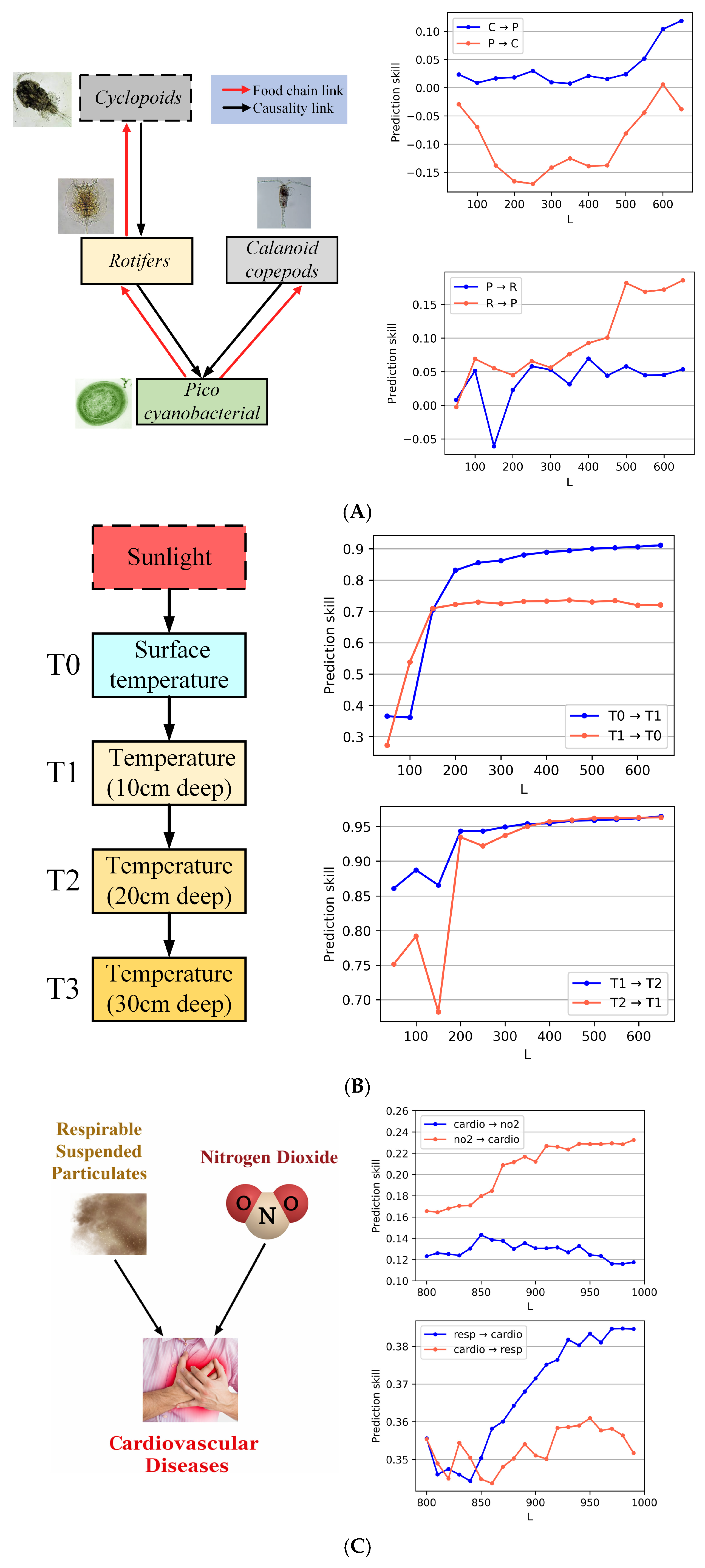
Firstly, we analyzed the food chain network of four plankton species: Picocyanobacterial, Calanoid copepods, Rotifers and Cyclopoids [35,36]. The oscillatory population data were extracted from an 8-year mesocosm experiment involving a plankton community [37,38]. The food chain relationships are shown in Figure 3A. In the food chain networks, the top-down control exerted by predators is significantly stronger than the bottom-up control exerted by prey [12], indicating a stronger causal relationship in the predator → prey direction. It is noted that a weak causal relationship may exist in the prey → predator direction; resultingly, the food chain networks can be viewed as scenario I in Figure 2. The direction of causality is opposite to that of the food chain link. We utilized data from three species, Picocyanobacterial (P), Calanoid copepods (C), and Rotifers (R) for causal analysis, while the data for Cyclopoids were regarded as unknown and only used for validating the results. Initially, we used the conventional CCM to analyze the causal relationships between prey and predator (Figure 3A). It can be observed that there exists a strong causal relationship in the C → P and R → P directions, and a weak causal relationship in the P → R direction, which is consistent with previous research [12].
Then we utilized DPE to analyze the causal relationships in the R → P and C → P directions, and the results are presented in the upper part of Table 2. In the R → P direction, the pairwise effect is observed, indicating that R may not be the most direct driver of P and implies the presence of a deep causal relationship (i.e., deep food chain link). Noticeably, Cyclopoids may represent a plausible upstream influence on R, even though Cyclopoids are regarded as unknown and unobservable in experiments. Moreover, no pairwise effect is observed in the C → P direction.
Secondly, we analyzed the causal networks among temperatures at different soil depths [39]. It is conventionally thought that environment factors such as sunlight and air influence surface soil temperature variations, while shallow soil temperatures serve as the cause for changes in deep soil layers. The causal networks are depicted in Figure 3B. In the experiments, we utilized the data of soil surface temperature (T0), temperature at depths of 10 cm (T1), 20 cm (T2), and 30 cm (T3) to analyze. The environmental data, such as air temperature and sunlight, were not available and we regarded them as unknown. From the prediction curves based on CCM, it suggested that variations in shallow soil temperatures drive changes in deep soil layers, aligning with soil science knowledge. Subsequently, we used DPE to analyze the causal relationships in the directions of T0 → T1, T1 → T2, and T2 → T3, with results presented in the middle part of Table 4. Noticeably, all these directions exhibited pairwise effects, suggesting that these causes (i.e., T0, T1, and T2, respectively) in these three directions may not be the most direct drivers of the results (i.e., T1, T2, and T3, respectively). Therefore, the results are consistent with the presence of deeper underlying factors in these directions (i.e., environmental factors, T1, and T2, respectively).
Thirdly, we investigated the data of air pollution and hospital admission of cardiovascular diseases in Hong Kong from 1994 to 1997 [38,40]. Relevant research has revealed that nitrogen dioxide and respirable suspended particulates were the two major causes of cardiovascular diseases [2], as shown in Figure 3C. Since DPE is to identify which pollutants cause cardiovascular disease and detect the potential deep causality, we fixed the disease as the target in the causal networks. Then we analyzed the data of nitrogen dioxide (N), respirable suspended particulates (resp) and cardiovascular diseases (cardio). From the prediction curves based on CCM, it suggested that there exist unidirectional causal relationships in resp → cardio and no2 → cardio directions. DPE revealed that pair effect is absent in resp → cardio direction. However, pair effect is present in no2 → cardio direction. The results suggested that nitrogen dioxide may not be the fundamental causes of cardiovascular diseases, and other pollutants may influence the nitrogen dioxide in the air. The conclusion is consistent with previous results [41,42].

4. Discussion

According to Takens’ embedding theorem, each variable in a dynamical system potentially carries information about the entire system. In principle, this provides a theoretical basis for recovering causal relationships from limited observations. In practice, however, ecological and environmental systems are shaped by multiple interacting drivers across scales, and the information contained in any single observed variable is often incomplete, noisy, or only weakly expressive of latent mechanisms [43]. As a result, extracting hidden causal structure from single-variable embeddings may be inefficient and may fail to reveal mediated or upstream influences.
To address this challenge, the proposed detecting pairwise effect (DPE) method extends conventional causality analysis by examining how predictive relationships change when multivariable information is incorporated. Rather than only confirming the presence of an observable causal link, DPE assesses whether such a link is more consistent with a direct causal driver or with a mediated relationship influenced by latent upstream variables. The emergence of the pairwise effect provides a diagnostic signal consistent with the possibility that an observed causal relationship (X → Y) embeds a deeper causal structure, such as a latent chain (Z → X → Y), in which X primarily acts as a mediator rather than the root cause of Y.
The effectiveness of DPE is supported by analyses of both simulated systems and real-world datasets. These results indicate that DPE can reveal patterns consistent with latent causal chains that may remain obscured under traditional causality inference methods based solely on observable variables. At the same time, the absence of a pairwise effect does not imply the absence of latent causal influences. Latent factors may exist but fail to produce a detectable signal when they influence multiple observed variables with comparable strength. Therefore, DPE should be interpreted as a diagnostic tool whose outcomes depend on the underlying causal configuration and the relative strengths of interactions.
From an ecological perspective, the ability to probe latent causal chains is particularly relevant, as many ecological systems are governed by partially observed drivers and multi-scale interactions. Observed variables often represent aggregated outcomes of multiple processes, including trophic interactions, density dependence, dispersal, and environmental forcing. Consequently, ecological time series frequently exhibit indirect causation, apparent bidirectionality, and regime shifts, where observed associations may reflect mediation through unmeasured upstream factors rather than direct interactions. In this context, DPE provides a practical way to assess whether an apparent link between two variables is more consistent with direct coupling or mediated influence.
The interpretation of the DPE signal depends on several conditions. First, the system should be sufficiently deterministic for state-space reconstruction to be meaningful, and the sampling resolution should be appropriate relative to the intrinsic timescale. Second, DPE is most informative when latent influences are asymmetric, such that upstream drivers affect one variable more strongly than another. Under such conditions, multivariable embedding may reduce the recoverability of one variable and lead to the pairwise effect. However, this behavior is not guaranteed. The DPE signal may become unreliable when common drivers affect both variables similarly, when strong synchrony or collinearity obscures directional information, or when nonstationarity, measurement noise, and limited sample size reduce the stability of predictive skill estimates. In this study, DPE is interpreted together with uncertainty quantification, including bootstrap confidence intervals and statistical testing, rather than relying solely on the sign of  Δ D P E .
In empirical applications, additional data-related factors may influence interpretation. Potential confounders (e.g., radiation, soil moisture, wind, boundary-layer dynamics) may simultaneously affect multiple variables, introducing indirect dependencies. Measurement errors and sensor noise may distort predictive skill, especially when differences in ρ are small. Moreover, inappropriate sampling intervals relative to system dynamics may degrade manifold reconstruction. These issues affect both CCM and DPE and should be considered when interpreting results. Preprocessing steps such as detrending, seasonal adjustment, and surrogate testing are recommended to improve robustness.
Despite these encouraging results, DPE still has important limitations. In particular, latent influences may remain difficult to diagnose when they affect multiple observed variables with similar strength or when causal pathways are highly entangled. DPE should therefore be viewed as complementary to existing causal inference approaches rather than as a replacement, and may be most useful when combined with methods designed to mitigate indirect effects or synchrony.

5. Conclusions

In this study, we proposed detecting pairwise effect (DPE), a data-driven method based on empirical dynamic modeling and multivariable state-space reconstruction, to assess whether an observed causal link is more consistent with a direct driver or with a mediated effect shaped by latent upstream forcing. Through analyses of benchmark systems and real-world datasets, we showed that DPE provides a diagnostic signal consistent with latent upstream influence that may not be directly observable in time series data. This improves the interpretability of inferred causal relationships in complex ecological and environmental systems.
However, DPE should be interpreted cautiously. Its performance depends on system properties, data quality, and the relative strength of causal interactions. In particular, common drivers, synchrony, nonstationarity, and limited sample size may affect the reliability of the inferred signal. Therefore, DPE is best used in conjunction with complementary methods and uncertainty quantification. Future work should further evaluate the robustness of DPE through systematic stress tests under varying noise levels, sampling conditions, and dynamical regimes, as well as through benchmarking against representative causal inference approaches. Such efforts will help to better characterize the applicability and limitations of DPE in real-world systems.

Supplementary Materials

The following supporting information can be downloaded at: https://www.mdpi.com/article/10.3390/a19040307/s1.

Author Contributions

Conceptualization, Z.C.; methodology, Z.C. and M.L.; software, Z.C.; validation, Z.C. and M.L.; formal analysis, Z.C. and M.L.; investigation, M.L.; data curation, Z.C. and M.L.; visualization, Z.C.; writing—original draft, Z.C.; writing—review and editing, Z.C. and M.L.; supervision, Z.C.; project administration, Z.C.; funding acquisition, Z.C. All authors have read and agreed to the published version of the manuscript.

Funding

This research was supported by the Natural Science Foundation of Shandong Province, China (Grant No. ZR2023QF131), the Enrolling Plan of Young Innovative Talents of Shandong Province (Grant No. 32, Big Data and Ecological Security Research and Innovation Team Project) and the Scientific Research Project of Zaozhuang University (Grant No. 21).

Data Availability Statement

The data and codes presented in this study are provided in the Supplementary Materials.

Conflicts of Interest

The authors declare no conflicts of interest.

References

  1. Leng, S.; Ma, H.; Kurths, J.; Lai, Y.C.; Lin, W.; Aihara, K.; Chen, L. Partial cross mapping eliminates indirect causal influences. Nat. Commun. 2020, 11, 2632. [Google Scholar] [CrossRef] [PubMed]
  2. Park, S.H.; Ha, S.; Kim, J.K. A general model-based causal inference method overcomes the curse of synchrony and indirect effect. Nat. Commun. 2023, 14, 4287. [Google Scholar] [CrossRef]
  3. Shojaie, A.; Fox, E.B. Granger causality: A review and recent advances. Annu. Rev. Stat. Appl. 2022, 9, 289–319. [Google Scholar] [CrossRef]
  4. Geweke, J.F. Measures of conditional linear dependence and feedback between time series. J. Am. Stat. Assoc. 1984, 79, 907–915. [Google Scholar] [CrossRef]
  5. Feng, J.; Fu, W.; Sun, F. Frontiers in Computational and Systems Biology; Springer: London, UK, 2010. [Google Scholar]
  6. Stankovski, T.; Duggento, A.; McClintock, P.V.E.; Stefanovska, A. A tutorial on time-evolving dynamical Bayesian inference. Eur. Phys. J. Spec. Top. 2014, 223, 2685–2703. [Google Scholar] [CrossRef]
  7. Cao, Z.; He, G.; Mu, S.; Qu, H. Effects of Bee Density and Hive Distribution on Pollination Efficiency for Greenhouse Strawberries: A Simulation Study. Agronomy 2023, 13, 731. [Google Scholar] [CrossRef]
  8. Cao, Z.; Shuo, J.; Qu, H. Strategies to enhance greenhouse strawberry yield through honeybee pollination behavior: A simulation study. Front. Plant Sci. 2024, 15, 1514372. [Google Scholar] [CrossRef]
  9. Coufal, D.; Jakubík, J.; Jajcay, N.; Hlinka, J.; Krakovská, A.; Paluš, M. Detection of coupling delay: A problem not yet solved. Chaos 2017, 27, 083109. [Google Scholar] [CrossRef]
  10. Ge, X.; Lin, A. Dynamic causality analysis using overlapped sliding windows based on the extended convergent cross-mapping. Nonlinear Dyn. 2021, 104, 1753–1765. [Google Scholar] [CrossRef]
  11. Johnson, B.; Munch, S.B. An empirical dynamic modeling framework for missing or irregular samples. Ecol. Model. 2022, 468, 109948. [Google Scholar] [CrossRef]
  12. Sugihara, G.; May, R.; Ye, H.; Hsieh, C.H.; Deyle, E.; Fogarty, M.; Munch, S. Detecting causality in complex ecosystems. Science 2012, 338, 496–500. [Google Scholar] [CrossRef]
  13. Ye, H.; Deyle, E.R.; Gilarranz, L.J.; Sugihara, G. Distinguishing time-delayed causal interactions using convergent cross mapping. Sci. Rep. 2015, 5, 14750. [Google Scholar] [CrossRef]
  14. Cummins, B.; Gedeon, T.; Spendlove, K. On the efficacy of state space reconstruction methods in determining causality. SIAM J. Appl. Dyn. Syst. 2015, 14, 335–381. [Google Scholar] [CrossRef]
  15. Harnack, D.; Laminski, E.; Schünemann, M.; Pawelzik, K.R. Topological causality in dynamical systems. Phys. Rev. Lett. 2017, 119, 098301. [Google Scholar] [CrossRef]
  16. Hlaváčková-Schindler, K.; Paluš, M.; Vejmelka, M.; Bhattacharya, J. Causality detection based on information-theoretic approaches in time series analysis. Phys. Rep. 2007, 441, 1–46. [Google Scholar] [CrossRef]
  17. Clark, A.T.; Ye, H.; Isbell, F.; Deyle, E.R.; Cowles, J.; Tilman, G.D.; Sugihara, G. Spatial convergent cross mapping to detect causal relationships from short time series. Ecology 2015, 96, 1174–1181. [Google Scholar] [CrossRef] [PubMed]
  18. Krakovská, A.; Hanzely, F. Testing for causality in reconstructed state spaces by an optimized mixed prediction method. Phys. Rev. E 2016, 94, 052203. [Google Scholar] [CrossRef] [PubMed]
  19. Suzuki, K.; Matsuzaki, S.I.S.; Masuya, H. Decomposing predictability to identify dominant causal drivers in complex ecosystems. Proc. Natl. Acad. Sci. USA 2022, 119, e2204405119. [Google Scholar] [CrossRef]
  20. Cobey, S.; Baskerville, E.B. Limits to causal inference with state-space reconstruction for infectious disease. PLoS ONE 2016, 11, e0169050. [Google Scholar] [CrossRef]
  21. Jiang, J.J.; Huang, Z.G.; Huang, L.; Liu, H.; Lai, Y.C. Directed dynamical influence is more detectable with noise. Sci. Rep. 2016, 6, 24088. [Google Scholar] [CrossRef]
  22. Kawatsu, K.; Ushio, M.; van Veen, F.F.; Kondoh, M. Are networks of trophic interactions sufficient for understanding the dynamics of multi-trophic communities? Analysis of a tri-trophic insect food-web time-series? Ecol. Lett. 2021, 24, 543–552. [Google Scholar] [CrossRef]
  23. Ye, L.; Tan, L.; Wu, X.; Cai, Q.; Li, B.L. Nonlinear causal analysis reveals an effective water level regulation approach for phytoplankton blooms controlling in reservoirs. Sci. Total Environ. 2022, 806, 150948. [Google Scholar] [CrossRef]
  24. Ushio, M.; Hsieh, C.H.; Masuda, R.; Deyle, E.R.; Ye, H.; Chang, C.W.; Sugihara, G.; Kondoh, M. Fluctuating interaction networks and time-varying stability of a natural fish community. Nature 2018, 554, 360–363. [Google Scholar] [CrossRef]
  25. Chen, W.; Cai, R.; Zhang, K.; Hao, Z. Causal discovery in linear non-Gaussian acyclic models with multiple latent confounders. IEEE Trans. Neural Netw. Learn. Syst. 2021, 33, 2816–2827. [Google Scholar] [CrossRef]
  26. Gilligan-Lee, C.M.; Hart, C.; Richens, J.; Johri, S. Leveraging directed causal discovery to detect latent common causes. IEEE Trans. Neural Netw. Learn. Syst. 2022, 35, 4938–4947. [Google Scholar] [CrossRef]
  27. Gerhardus, A.; Runge, J. High-recall causal discovery for autocorrelated time series with latent confounders. Adv. Neural Inf. Process. Syst. 2020, 33, 12615–12625. [Google Scholar]
  28. Takens, F. Detecting strange attractors in turbulence. In Dynamical Systems and Turbulence; Springer: Berlin/Heidelberg, Germany, 2006; pp. 366–381. [Google Scholar] [CrossRef]
  29. Deyle, E.R.; Sugihara, G. Generalized theorems for nonlinear state space reconstruction. PLoS ONE 2011, 6, e18295. [Google Scholar] [CrossRef] [PubMed]
  30. McCracken, J.M.; Weigel, R.S. Convergent cross mapping and pairwise asymmetric inference. Phys. Rev. E 2014, 90, 062903. [Google Scholar] [CrossRef]
  31. Ye, H.; Sugihara, G. Information leverage in interconnected ecosystems: Overcoming the curse of dimensionality. Science 2016, 353, 922–925. [Google Scholar] [CrossRef] [PubMed]
  32. Dixon, P.A.; Milicich, M.J.; Sugihara, G. Episodic fluctuations in larval supply. Science 1999, 283, 1528–1530. [Google Scholar] [CrossRef]
  33. Sugihara, G.; May, R.M. Nonlinear forecasting as a way of distinguishing chaos from measurement error in time series. Nature 1990, 344, 734–741. [Google Scholar] [CrossRef]
  34. Chang, C.W.; Ushio, M.; Hsieh, C.H. Empirical dynamic modeling for beginners. Ecol. Res. 2017, 32, 785–796. [Google Scholar] [CrossRef]
  35. Liebert, W.; Schuster, H.G. Proper choice of the time delay for the analysis of chaotic time series. Phys. Lett. A 1989, 142, 107–111. [Google Scholar] [CrossRef]
  36. Benincà, E.; Huisman, J.; Heerkloss, R.; Jöhnk, K.D.; Branco, P.; Van Nes, E.H.; Scheffer, M.; Ellner, S.P. Chaos in a long-term experiment with a plankton community. Nature 2008, 451, 822–825. [Google Scholar] [CrossRef]
  37. Benincà, E.; Jöhnk, K.D.; Heerkloss, R.; Huisman, J. Coupled predator–prey oscillations in a chaotic food web. Ecol. Lett. 2009, 12, 1367–1378. [Google Scholar] [CrossRef]
  38. Lee, B.J.; Kim, B.; Lee, K. Air pollution exposure and cardiovascular disease. Toxicol. Res. 2014, 30, 71–75. [Google Scholar] [CrossRef]
  39. Cao, Z.; Mu, S.; Xu, L.; Shao, M.; Qu, H. Causal research on soil temperature and moisture content at different depths. IEEE Access 2021, 9, 39077–39088. [Google Scholar] [CrossRef]
  40. Wong, T.W.; Lau, T.S.; Yu, T.S.; Neller, A.; Wong, S.L.; Tam, W.; Pang, S.W. Air pollution and hospital admissions for respiratory and cardiovascular diseases in Hong Kong. Occup. Environ. Med. 1999, 56, 679–683. [Google Scholar] [CrossRef]
  41. Milojevic, A.; Wilkinson, P.; Armstrong, B.; Bhaskaran, K.; Smeeth, L.; Hajat, S. Short-term effects of air pollution on a range of cardiovascular events in England and Wales: Case-crossover analysis of the MINAP database, hospital admissions and mortality. Heart 2014, 100, 1093–1099. [Google Scholar] [CrossRef]
  42. Peng, R.D.; Chang, H.H.; Bell, M.L.; McDermott, A.; Zeger, S.L.; Samet, J.M.; Dominici, F. Coarse Particulate Matter Air Pollution and Hospital Admissions for Cardiovascular and Respiratory Diseases Among Medicare Patients. JAMA 2008, 299, 2172–2179. [Google Scholar] [CrossRef] [PubMed]
  43. Cao, Z.; Jiang, Z.; Liu, G.; Wang, Y.; Qu, H. Why does strawberry fruit weight distribution show positive skewness? A simulation model reveals the underlying processes of fruit production. Front. Plant Sci. 2023, 14, 1255724. [Google Scholar] [CrossRef] [PubMed]
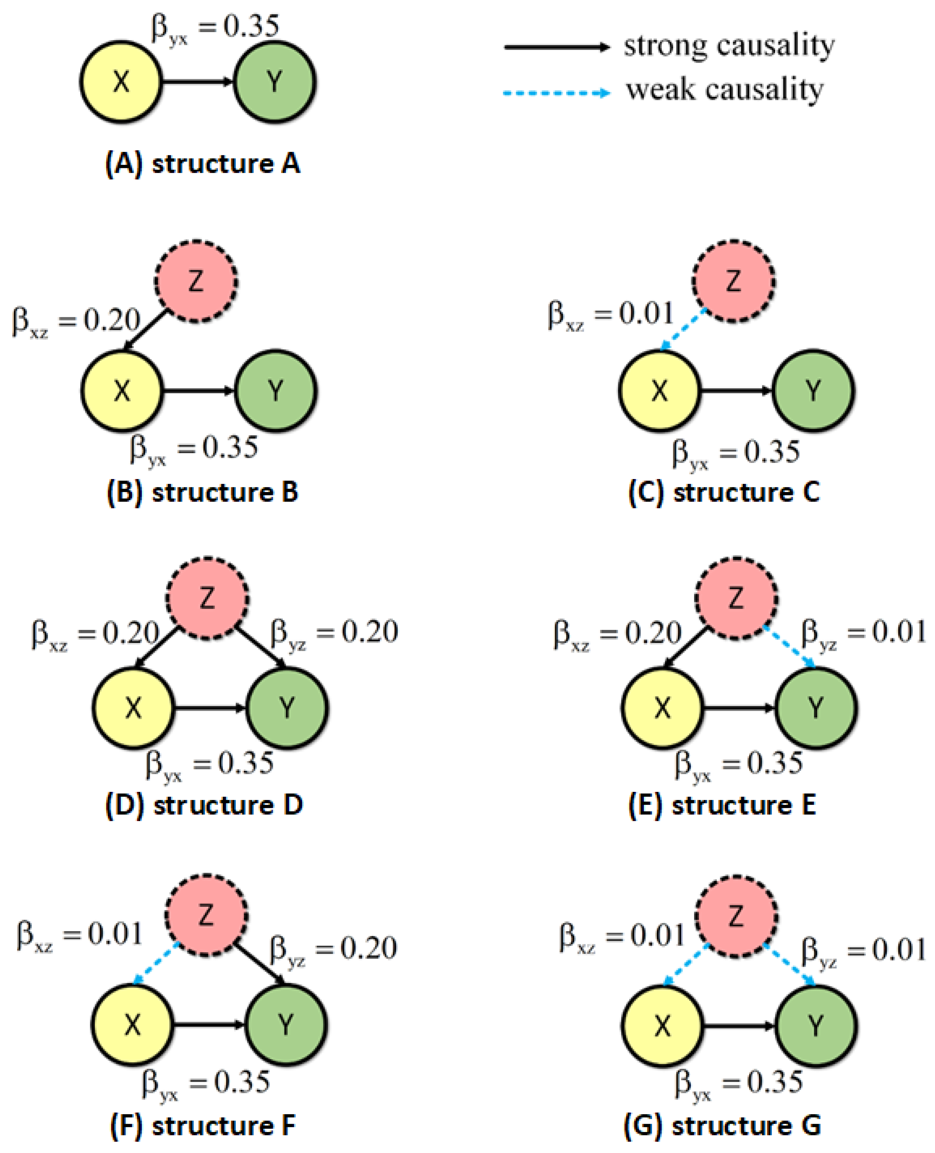
Figure 1. Seven distinctive causal network structures. These causal networks include three variables: X, Y, and Z. A unidirectional strong causal relation X → Y is fixed. Black arrows represent strong causal relationships ( β = 0.20 ), while blue arrows indicate weak causal relationships ( β = 0.01 ). Here,  β y x  represents the causal strength in the X → Y direction,  β y x  represents the causal strength in the Z → X direction, and  β x z  represents the causal strength in the Z → Y direction.
Algorithms 19 00307 g001
Figure 2. Sensitivity analysis results of DPE. (A) Causal network of Z → X → Y with different values of  β x z . When the value of the blue curve surpassed the red curve, the pairwise effect was present. (B) Causal network of Z → X → Y and Z → Y with different values of  β y z . When the value of the blue curve surpasses the red curve, the pairwise effect is present. (C) Two proposed scenarios with bidirectional causality between X and Y. In this panel, the black arrows indicate strong causal relationships, whereas the red dashed arrows indicate weak causal relationships. In scenario H, Z has no impact on X and Y. In scenario I, Z exhibits a strong causal relationship with X. (D) DPE analysis results for scenario H. When the value of the blue curve surpasses that of the red curve, a pairwise effect is observed. (E) Experimental results for scenario I. When the value of the blue curve surpasses that of the red curve, a pairwise effect manifests.
Algorithms 19 00307 g002
Figure 3. Detecting possible latent causation in three real-world networks. (A) The food chain and causal relationship in prey-predator system. The direction of causality contradicts that of the food chain link. The prediction skill shows strong causal relationships in C → P and R → P directions. (B) Causal relationships among temperatures at different soil depths. The prediction skills signify strong causal relationships in T0 → T1 and T1 → T2 directions. (C) Verified causal networks of cardiovascular diseases. Nitrogen dioxide and respirable suspended particulates are the two major causes of cardiovascular diseases.
Algorithms 19 00307 g003
Table 1. Experimental results for scenarios A–G.
Scenario   ρ X , X ^ M x + y   ρ Y , Y ^ M y + x   Δ D P E 95% CI
of   Δ D P E  
p-ValuePairwise Effect
A0.9999090.999725>0[0.00011, 0.00025]<0.001-
B0.9992550.999511<0[−0.00034, −0.00018]<0.001
C0.9998630.999743>0[0.00034, 0.00018]<0.001-
D0.9994230.999097>0[0.00024, 0.00041]0.002-
E0.9992260.999489<0[−0.00035, −0.00019]<0.001
F0.9998420.999158>0[0.00057, 0.00080]<0.001-
G0.9998890.999752>0[0.00007, 0.00021]0.001-
“★” indicates the presence of pairwise effect and “-” indicates the absence of pairwise effect.
Table 2. Robustness to observation noise.
ScenarioNoise Level σ   Δ D P E   95 %   CI   of   Δ D P E Pairwise Effect
Interpretation
A0.000.00018[0.00011, 0.00025]no supported
A0.010.00015[0.00007, 0.00023]no supported
A0.050.00008[−0.00001, 0.00017]no supported
A0.100.00003[−0.00010, 0.00015]inconclusive
B0.00−0.00026[−0.00034, −0.00018]supported
B0.01−0.00022[−0.00031, −0.00013]supported
B0.05−0.00011[−0.00031, −0.00013]supported
B0.10−0.00005[−0.00017, 0.00006]inconclusive
Table 3. Robustness to time-series length.
Scenario   Library   Length   L   Δ D P E   95 %   CI   of   Δ D P E Pairwise Effect
Interpretation
A15000.00018[0.00011, 0.00025]no supported
A10000.00015[0.00007, 0.00023]no supported
A5000.00008[−0.00001, 0.00017]no supported
A2500.00003[−0.00010, 0.00015]inconclusive
B1500−0.00026[−0.00034, −0.00018]supported
B1000−0.00022[−0.00031, −0.00013]supported
B500−0.00011[−0.00031, −0.00013]supported
B250−0.00005[−0.00017, 0.00006]inconclusive
Table 4. Experimental results for real-world systems.
Direction   ρ C , C ^ M C + P   ρ P , P ^ M P + C   Δ D P E 95% CI
of   Δ D P E  
p-valuePairwise
effect
C → P0.9942460.988015 > 0 [0.00490, 0.00743]<0.001-
Direction   ρ R , R ^ M R + P   ρ P , P ^ M P + R   Δ D P E 95% CI
of   Δ D P E  
p-valuePairwise
effect
R → P0.9864010.989355 < 0 [−0.00418, −0.00173]<0.001
Direction   ρ T 0 , T 0 ^ M T 0 + T 1   ρ T 1 , T 1 ^ M T 1 + T 0   Δ D P E 95% CI
of   Δ D P E  
p-valuePairwise
effect
T0 → T10.9951960.998239 < 0 [−0.00411, −0.00196]<0.001
Direction   ρ T 1 , T 1 ^ M T 1 + T 2   ρ T 2 , T 2 ^ M T 2 + T 1   Δ D P E 95% CI
of   Δ D P E  
p-valuePairwise
effect
T1 → T20.9983130.998774 < 0 [−0.00102, 0.00009]0.086
Direction   ρ T 2 , T 2 ^ M T 2 + T 3   ρ T 3 , T 3 ^ M T 3 + T 2   Δ D P E 95% CI
of   Δ D P E  
p-valuePairwise
effect
T2 → T30.9987370.999044 < 0 [−0.00081, 0.00013]0.119
Direction   ρ R e , R e ^ M R e + C a   ρ C a , C a ^ M C a + R e   Δ D P E 95% CI
of   Δ D P E  
p-valuePairwise
effect
Re → Ca0.9907860.98799 > 0 [0.00152, 0.00401]<0.001-
Direction   ρ N , N ^ M N + C a   ρ C a , C a M C a + N   Δ D P E 95% CI
of   Δ D P E  
p-valuePairwise
effect
N → Ca0.9835260.985287 < 0 [−0.00291, −0.00064]0.003
“★” indicates the presence of pairwise effect and “-” indicates the absence of pairwise effect.
Disclaimer/Publisher’s Note: The statements, opinions and data contained in all publications are solely those of the individual author(s) and contributor(s) and not of MDPI and/or the editor(s). MDPI and/or the editor(s) disclaim responsibility for any injury to people or property resulting from any ideas, methods, instructions or products referred to in the content.