Robust Prediction of Compressive Strength of SCM Concrete with Nested Cross-Validation and Bayesian Optimization

Abstract

Concrete production is one of the main sources of CO₂ emissions. The primary reason for this is the high clinker content of Portland cement. To mitigate this problem, supplementary cementitious materials (SCMs) such as fly ash, silica fume, Ground granulated blast furnace slag (GGBFS), rice husk ash, and natural pozzolans are increasingly being used. These materials are used as partial replacements for cement. SCMs not only reduce the environmental impact of concrete but can also improve its long-term mechanical and durability properties. The aim of this study is to develop a machine learning framework that can accurately predict the compressive strength of concrete containing SCMs. The framework includes the training and evaluation of several machine learning models. Nested cross-validation and Bayesian hyperparameter optimization were used to explore the full capacity of the models and ensure reliable evaluation. Permutation significance testing and learning curve analysis were applied to verify that the models learn meaningful patterns rather than memorize the data. Also, feature importance and SHapley Additive exPlanations analyses were performed and the key variables that influence the prediction of the compressive strength of SCM concrete were identified. The optimized XGBoost model achieved the best generalization performance with a holdout R² of 0.8398. It confirms the effectiveness of the proposed statistically rigorous machine learning framework for reliable compressive strength prediction of SCM-blended concrete.

1. Introduction

The concept of sustainability in the built environment revolves around conserving resources. It evaluates life cycle costs and designs for human comfort and usability. In terms of resource conservation, the 3Rs approach (Reduce, Reuse, and Recycle) is widely adopted within both construction and manufacturing industries [1]. As is known, concrete is a key building material due to its adaptability and design flexibility. Its embodied CO₂ mainly depends on the cement content with concrete producing about 100 kg of CO₂ per tonne on average. Since Portland cement is the main source of these emissions, reducing its use is the main essential key. Partial replacement with Supplementary Cementitious Materials (SCMs) such as Ground Granulated Blast Furnace Slag (GGBS), Pulverized Fly Ash (PFA), Rice Husk Ash (RHA), and Silica Fume (SF) can significantly lower the carbon footprint. SCMs are initially used to reduce costs, but now they are widely used to enhance the sustainability of concrete by decreasing CO₂ emissions [2]. SCMs have long been integrated into concrete either as partial substitutes for clinker in cement or as replacements for a portion of cement in concrete mixtures. This approach benefits the industry by generally reducing costs, minimizing environmental impacts and enhancing both strength and durability.

Machine learning is particularly valuable for SCM-based concrete because the interactions between cement, supplementary materials, water content and curing conditions are highly nonlinear and difficult to represent using conventional empirical equations. By learning complex relationships directly from experimental datasets, machine learning models can provide more reliable and generalized predictions of compressive strength across diverse material compositions. Recently, several machine learning approaches have been proposed for SCMs. The related studies are mentioned as follows:

Sobuz et al. experimentally investigated the mechanical and durability properties of high-strength self-compacting concrete containing marble powder, fly ash, and silica fume, and used machine learning models to predict these properties. The results show that appropriate SCM ratios can increase the strength of concrete while reducing environmental impacts [3].

Moradi et al. investigated the mechanical effects of binary admixtures used in the concrete industry and developed a machine learning-based model to predict the compressive strength of concrete containing these materials. The proposed model can accurately predict the compressive strength of concrete with different SCM combinations and allows the determination of optimum binary SCM ratios [4].

Liu et al. modeled the creep behavior of additive-modified concrete using machine learning methods and analyzed the factors affecting this behavior. In the study, creep prediction models were developed using Linear Regression (LR), Support Vector Regression (SVR), Random Forest (RF), and Extreme Gradient Boosting (XGB) models. Parameter sensitivity was examined using SHapley Additive exPlanations (SHAP) analysis and the results showed that the XGB model could predict the creep fit of SCM concrete with high accuracy [5].

Ahmad et al. [6] comparatively investigated machine learning methods such as bagging, AdaBoost, gene expression programming and decision tree to predict the compressive strength of concrete containing fly ash and blast furnace slag. The results show that the bagging model can predict the compressive strength of concrete with high accuracy (R² ≈ 0.92) and that ML methods can save time and resources in the concrete design process.

Miao et al. [7] used hybrid machine learning algorithms to predict the mechanical properties of concrete with recycled aggregate and admixtures. The results show that the SSA-XGB hybrid model can predict compressive, flexural and tensile strength and modulus of elasticity with high accuracy. Water/binder ratio, cement content, and superplasticizer amount are the most effective parameters.

Tran [8] comparatively investigated various machine learning algorithms to predict the chloride diffusion coefficient of concrete containing additives. The results show that the Gradient Boosting model provides the highest prediction performance. The basic parameters affecting chloride diffusion can be determined by using SHAP, Individual Conditional Expectation (ICE) and Partial Dependence Plot (PDP) analyses.

Kurniati et al. [9] developed machine learning models to predict the compressive strength of cement paste using copper mine waste as an admixture. The results show that the Random Forest model can predict compressive strength with high accuracy for different mix ratios and curing times, and that this approach can contribute to sustainable cement design.

Datta et al. [10] investigated the mechanical properties, microstructural behavior and environmental impacts of concrete using rice husk ash as an admixture using experimental and machine learning approaches. The results show that approximately 15% RHA substitution provides optimal strength and environmental performance. The XGBoost model offers high accuracy in predicting concrete properties.

Yoon et al. [11] used machine learning models to predict the reactivity of different admixtures depending on their physical and chemical properties. The results show that the artificial neural network (ANN) model provides the highest prediction accuracy. The important parameters can be determined in predicting SCM reactivity.

Golafshani et al. [12] proposed a framework integrating machine learning models with optimization algorithms to improve low-carbon mix design for concrete with recycled aggregates and admixtures. The results show that the CatBoost, XGBoost, and LightGBM models successfully predict the strength and durability properties of concrete. The proposed approach significantly reduces the carbon footprint.

Alkharisi and Dahish [13] used Response Surface Methodology (RSM) and machine learning models (M5P, Random Forest, XGBoost) together to predict the compressive strength of concrete with recycled aggregates and admixtures. The results show that the XGBoost model provides the highest prediction accuracy. Curing age and superplasticizer amount are the most influential parameters on compressive strength.

Chen et al. [14] comparatively investigated various machine learning models to predict the compressive strength of concrete with recycled aggregates containing fly ash and blast furnace slag. The results show that the particle swarm optimization-based backpropagation model provides the highest prediction accuracy, while curing age and cement content are the most important parameters determining strength development.

Sathiparan et al. [15] combined machine learning models with chemical composition data to predict the compressive strength of permeable concrete containing admixtures. The results show that the XGBoost model provides high prediction accuracy. CaO, SiO₂ content, and curing time are critical parameters in strength prediction.

Parhi and Patro [16] combined machine learning with multi-objective optimization to predict and optimize the compressive strength, porosity, and cost of admixture concrete. The results show that the Random Forest model provides high accuracy in strength prediction (R² = 0.97). the multilayer perceptron model provides high accuracy in porosity prediction (R² = 0.96). The developed models allow for the determination of practical mix designs with Multi-Objective Differential Evolution Optimizer and a user-friendly graphical user interface (GUI).

Abbas and Muntean [17] used artificial neural networks (ANN) to predict the tensile strength of concrete containing waste-derived admixtures. The ANN model, which is optimized via the Levenberg–Marquardt algorithm, provided predictions with high accuracy (R = 1) and low MSE over 440 data points. The study shows that while SCMs improve concrete durability and environmental performance, the ANN-based approach can reduce the need for physical testing and accelerate sustainable mix design.

Although many current studies have successfully applied machine learning to predict the properties of concrete containing SCM, the complex nonlinear interactions between mix parameters and the need for reliable generalization highlight the importance of developing robust and statistically reliable machine learning frameworks. The key innovation of this study is the development of a statistically robust and fully integrated machine learning framework for predicting the compressive strength of SCM-blended concrete. This framework also aims to provide reliable generalization and interpretability.

Unlike many previous studies, this research does not rely solely on traditional cross-validation or simple training-test data separation. Instead, it employs a nested cross-validation architecture combined with Bayesian hyperparameter optimization to provide a clear separation between model tuning and performance evaluation. Furthermore, permutation-based significance tests are applied to verify that model performance stems from genuine input–output relationships, not random correlations or overfitting. In addition, a SHAP-based explainable artificial intelligence approach is used to transparently interpret the effect of mix components on strength prediction. The developed framework was validated using a large global dataset containing 1456 SCM concrete mixes. The results show that the proposed method is robust and reliable for data-driven strength prediction.

Recent studies have also increasingly focused on combining predictive accuracy with interpretability in machine learning-based modeling. For instance, interpretable surrogate models based on Random Forest algorithms, combined with SHAP analysis, have been proposed to explain model predictions while maintaining high accuracy [18].

In addition, several recent studies have explored advanced data-driven and hybrid learning frameworks, including multi-source data-driven models, hybrid machine learning approaches, and deep learning architectures such as CNN-LSTM optimized using Bayesian techniques [19,20,21]. These developments highlight a growing trend toward more robust, interpretable, and data-efficient predictive systems.

Compared to these recent advances, the present study integrates nested cross-validation, Bayesian hyperparameter optimization, permutation significance testing, and SHAP-based interpretability within a unified framework. This combination provides not only strong predictive performance but also improved statistical reliability and model transparency.

2. Materials and Methods

A large-scale global dataset was curated from the study “A Global Dataset of SCM-Blended Concrete and Its Properties” by Liu et al. [22] that was available on Mendeley Data. This dataset encompasses variables such as cement, water, fly ash, coarse aggregate, silica fume, ground granulated blast furnace slag (GGBFS) and superplasticizer for concrete mix proportion [23].

The methodology starts with exploratory data analysis, following this with a set of machine learning models that were evaluated using nested cross-validation and hyperparameter optimization. Then, a feature importance analysis and an SHAP analysis were performed on the best-performing models. Finally, the study concludes with permutation significance testing and learning curve analysis proving the models’ learning as genuine but not memorization of data.

2.1. The Dataset

2.1.1. Exploratory Data Analysis

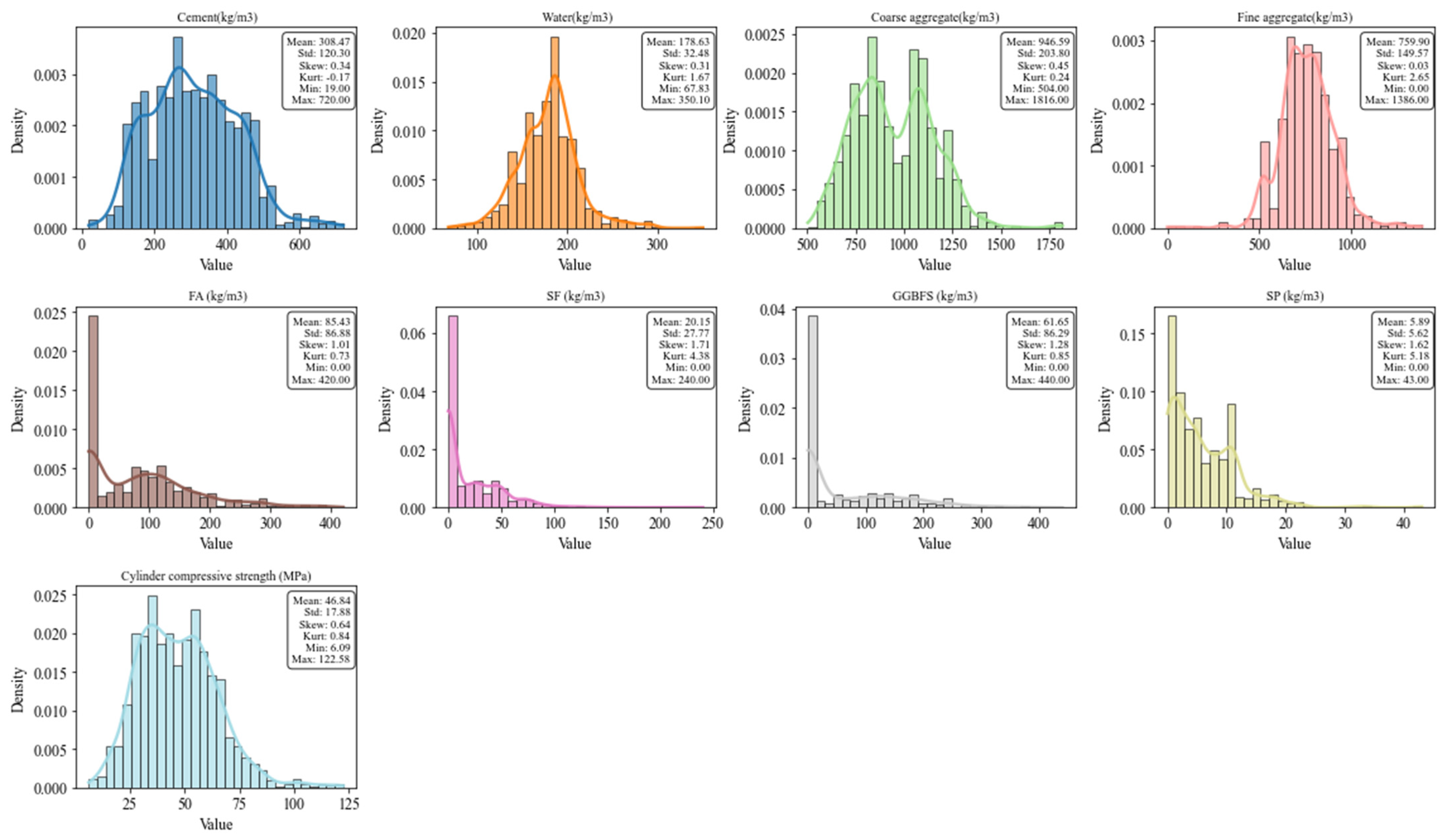
The dataset size is 1456 × 9. This dataset consists of 8 independent variables and 1 target variable (Cylinder Compressive Strength). The input variables are cement, fly ash, water, superplasticizer, coarse aggregate, fine aggregate, silica fume, and ground granulated blast furnace slag. Figure 1 shows the distribution of each variable with histogram graphs. In addition to the histograms, kernel density estimation (KDE) curves are also provided. Descriptive statistics are also presented in each histogram. These are minimum and maximum values, mean (µ), standard deviation (σ), skewness (β), and kurtosis (γ).

2.1.2. Correlation Analysis

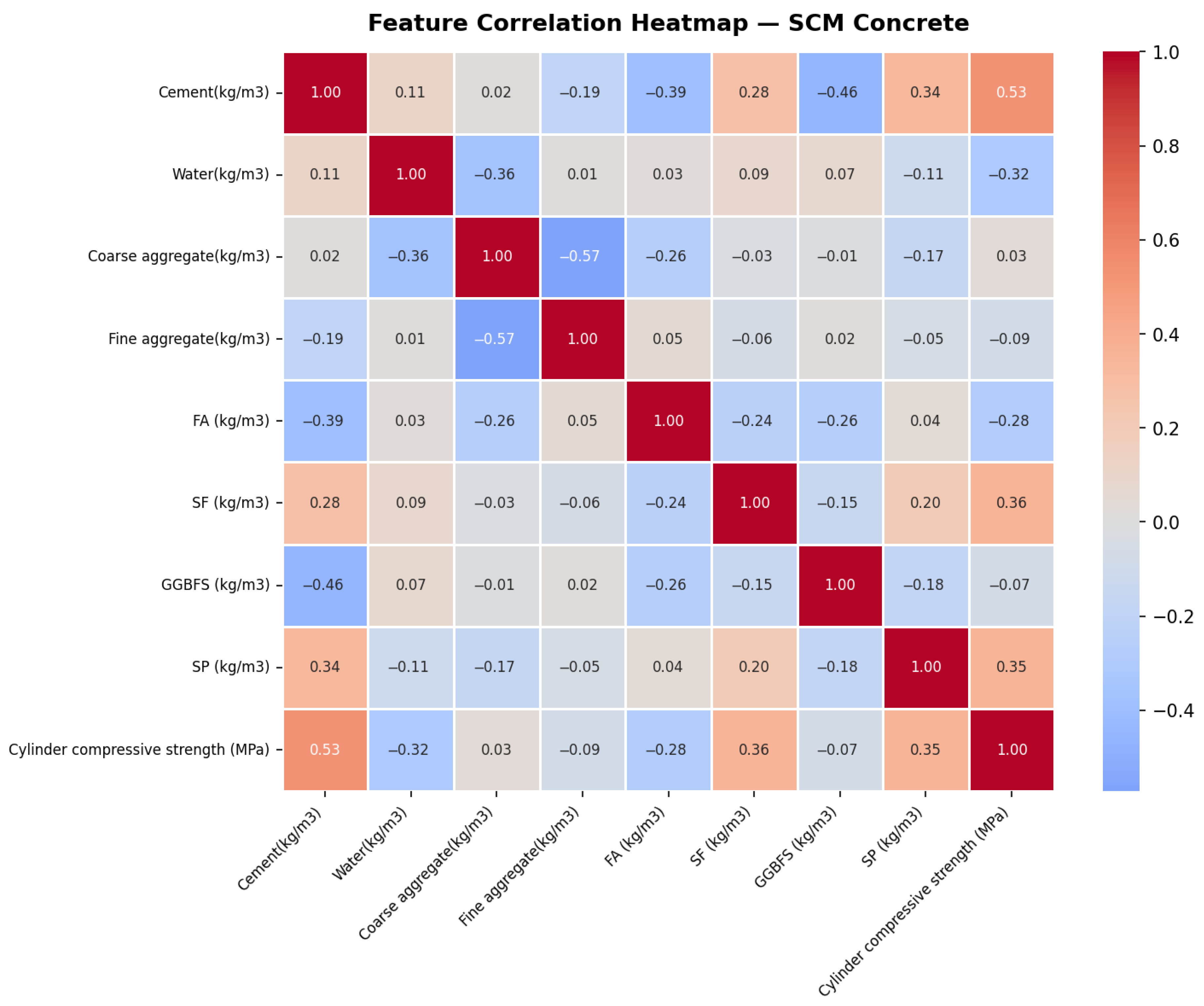
The correlation matrix shown in Figure 2 summarizes the linear relationships between concrete mix parameters and the obtained compressive strength. The correlation values shown in the matrix were derived from the dataset as Pearson correlations between features. This matrix, showing pairwise correlation coefficients, reveals how strongly each input variable relates to other variables. Therefore, it is a useful tool for identifying multicollinearity, understanding parameter interactions, and guiding feature selection for modeling. On this scale, values close to +1 indicate strong positive correlation. Values close to −1 indicate strong negative correlation. Coefficients close to zero indicate weak or no linear relationships.

As seen in Figure 2, there are clear reciprocal relationships between some mix components. For example, there is a clear positive correlation between cement and compressive strength. The water variable, however, shows a weak negative trend with both aggregates and strength. Similarly, coarse and fine aggregates show a moderate negative correlation with some binder materials. This indicates opposing interaction trends within the mix design.

2.2. Machine Learning Methods

In this study, machine learning (ML) techniques were applied using a comprehensive global dataset to model and predict the mechanical properties of concretes containing SCMs. Algorithms were trained and tuned on mixtures with different binder types and varying cementitious component ratios.

Each model underwent a careful hyperparameter optimization process to reduce prediction errors and improve generalization performance. Comparing the outputs of the models provides important insights into the ability of ensemble learning approaches to capture complex interactions between material components and accurately predict compressive strength. A brief introduction to each model used in the training and evaluation process is given below.

2.2.1. K Nearest Neighbors

One of the employed algorithms, K-Nearest Neighbors (KNN), is a non-parametric and instance-based learning approach that can be applied to both classification and regression problems. In this method, the value of a new observation is determined based on the closest data points in the training set using a selected distance metric. Although various distance measures can be used, Euclidean distance is the most common [24]. For regression tasks, KNN estimates the output by averaging the values of the k nearest neighbors, and the choice of k significantly influences model performance.

In this study, the KNN model was implemented using the Scikit-learn library within the proposed nested cross-validation framework. The mathematical formulation of the KNN method is given below:

$$\widehat{y}={\displaystyle \frac{1}{k}}{\sum }_{i=1}^k{ y}_i,$$

(1)

2.2.2. Multilayer Perceptron

Artificial Neural Networks (ANNs) have been widely used since the 1990s. Their prediction performance is influenced by several factors, including the selected input variables, network architecture, activation functions, and training algorithm [25]. Among different ANN structures, the Multilayer Perceptron (MLP) is commonly used due to its flexibility and wide range of applications [26]. However, the Levenberg–Marquardt (LM) algorithm, often used for training MLP models, may face limitations when applied to highly complex datasets [27]. More details on MLP structures can be found in Taud and Mas [28].

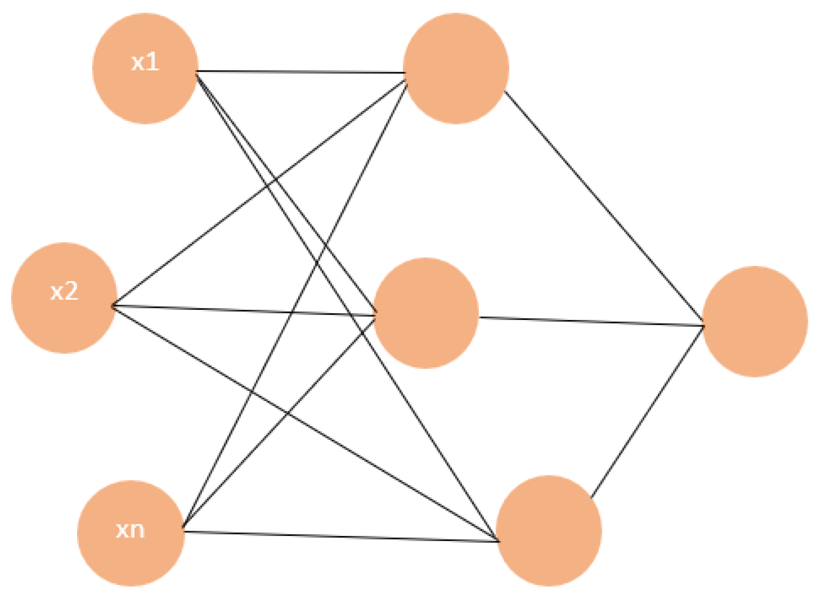
The MLP model was implemented within the proposed framework. A schematic representation of the MLP structure is shown in Figure 3.

2.2.3. Support Vector Machine

Another employed algorithm, Support Vector Machine (SVM), is regarded as one of the key algorithms in machine learning. Its strength lies in its capacity to identify classification patterns with reliable accuracy and consistent performance. While it can also be applied to certain regression tasks, SVM is predominantly recognized today as a robust and widely adopted method for classification problems [29].

2.2.4. ElasticNet

The used algorithm called Elastic Net Regression [30] is a regularization technique that combines Lasso (L1) and Ridge (L2) penalties to address multicollinearity and reduce overfitting in high-dimensional datasets. Its mathematical formulation is expressed as follows:

y = b0 + b1 × x1 + b2 × x2 + … + bn × xn + e,

(2)

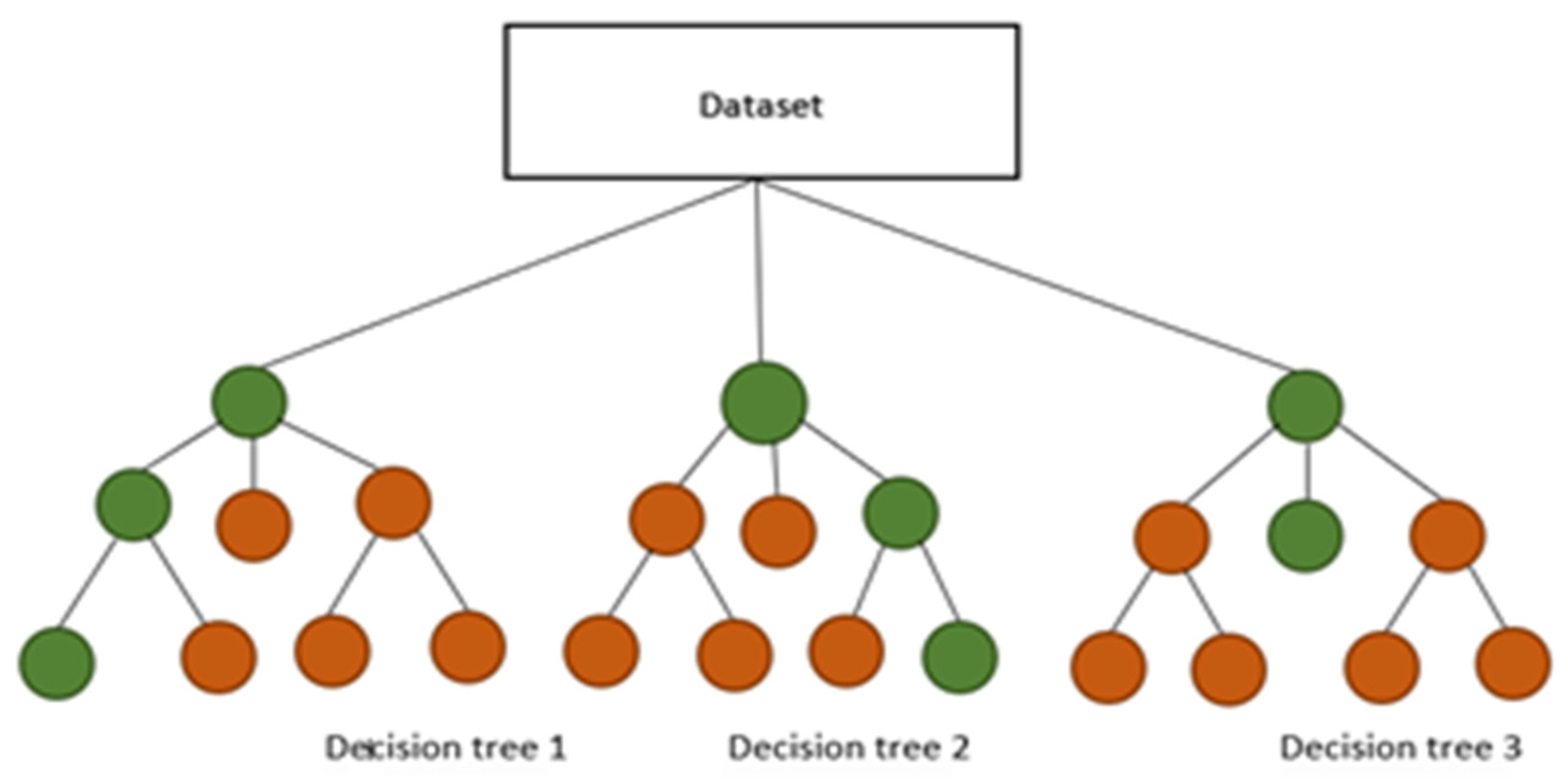
2.2.5. Decision Tree

Decision Trees (DTs) [31] were also employed in this study. These models are hierarchical structures widely used for classification and regression tasks, where decisions are made sequentially based on input features. Compared to neural networks, DTs offer a simpler and more interpretable structure.

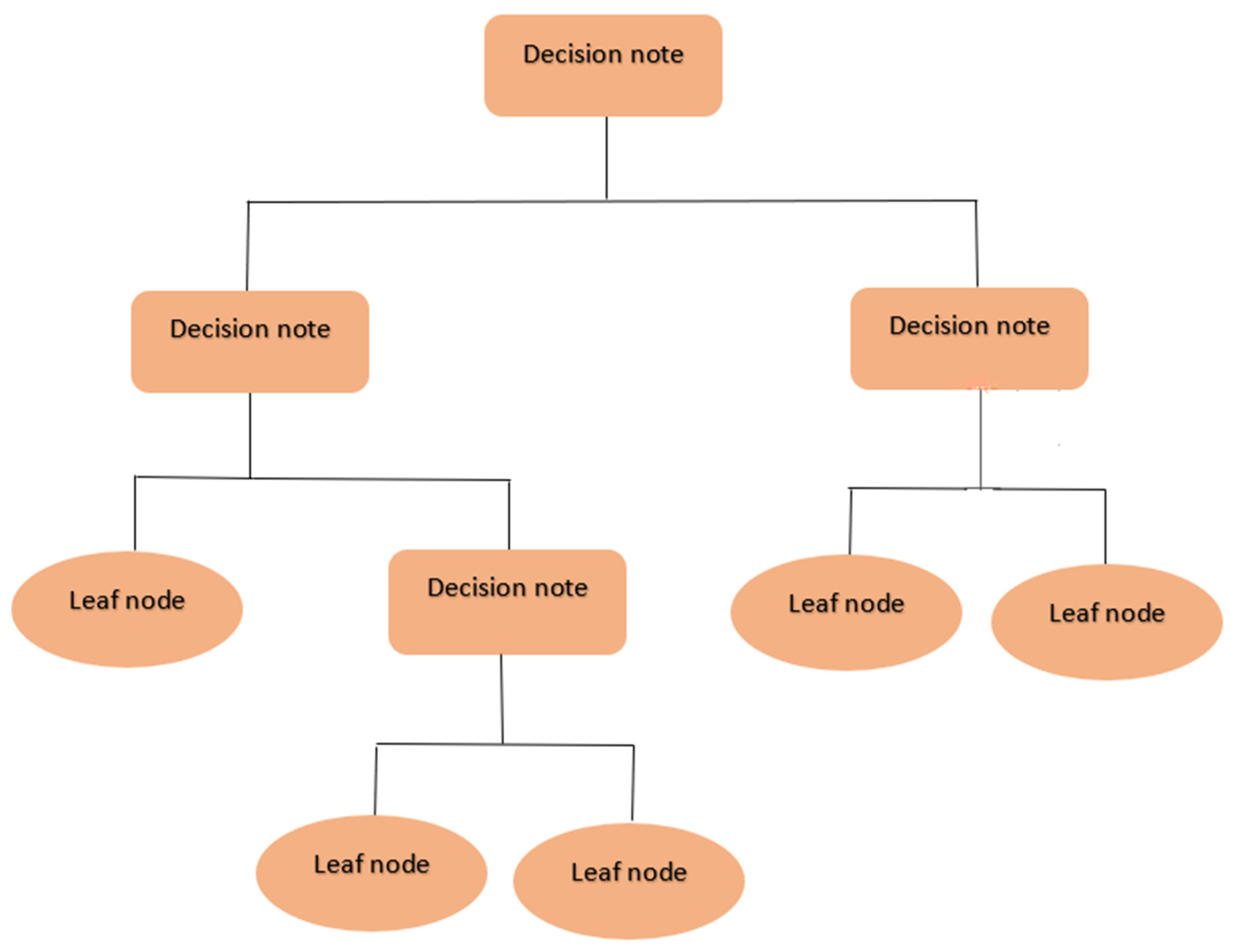
The Decision Tree model was implemented within the proposed framework. A schematic representation of the DT structure is shown in Figure 4.

2.2.6. Bagging

Bagging (bootstrap aggregation) is an ensemble learning technique that generates multiple versions of a base model by training on different bootstrap samples and combining their outputs. For regression tasks, predictions are averaged, while for classification, a majority voting scheme is used. This approach is particularly effective for reducing variance and improving the stability of models that are sensitive to variations in the training data [32]. In this study, the Bagging approach was implemented using Decision Trees as base learners.

2.2.7. Random Forest

The Random Forest (RF) algorithm is a widely used ensemble method for both classification and regression tasks [33]. It constructs multiple decision trees using randomly sampled subsets of the data and combines their outputs through averaging or majority voting [34,35]. RF is known for its robustness against overfitting and its ability to handle high-dimensional datasets, although it may require careful hyperparameter tuning [36].

In this study, the Random Forest model was implemented within the proposed framework. A schematic representation of the RF structure is shown in Figure 5. The node colors indicate variations in the predicted continuous values in the regression trees.

2.2.8. Extreme Gradient Boosting (XGBoost)

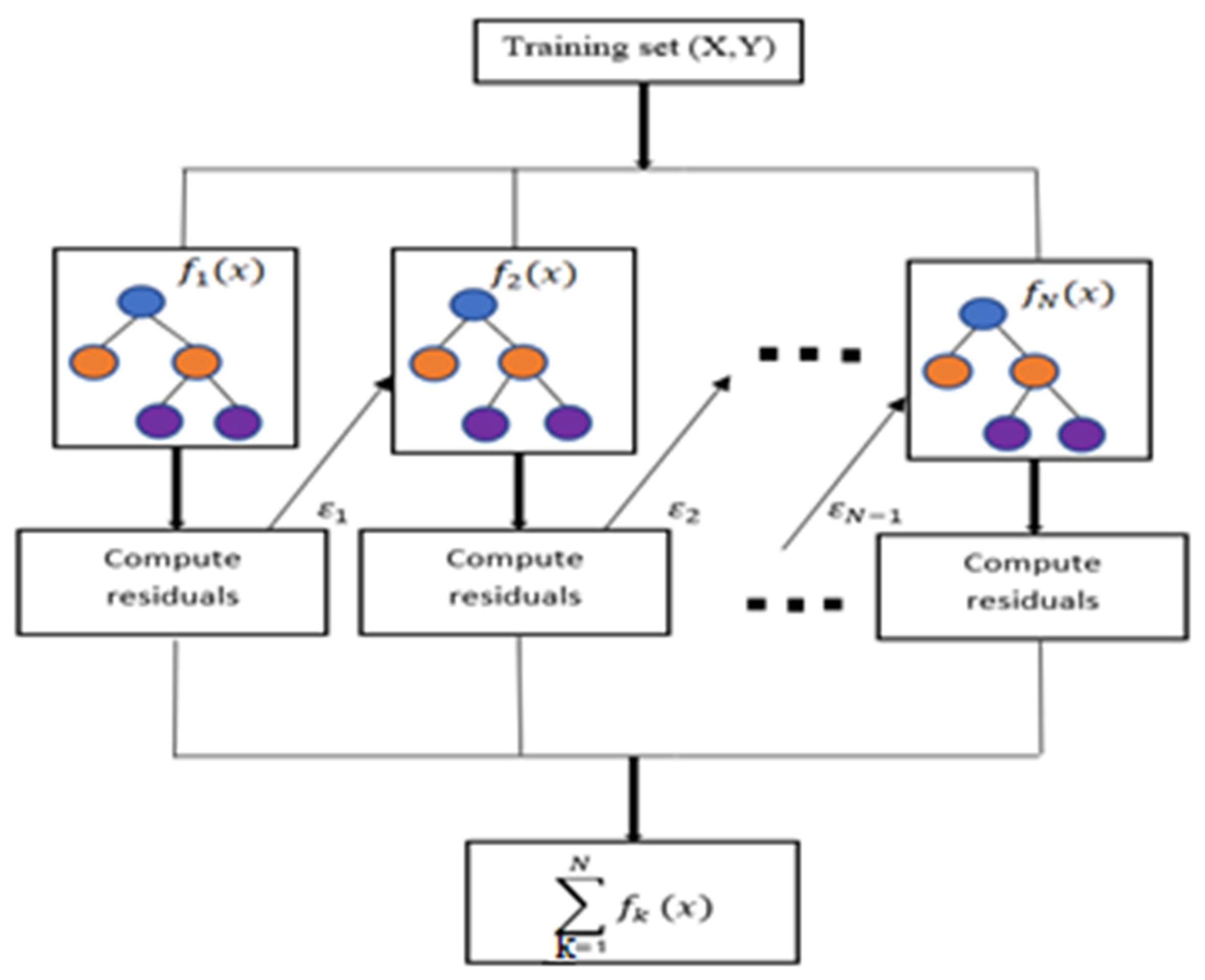
XGBoost is an ensemble learning algorithm based on decision trees, where multiple trees are constructed sequentially, and each tree is trained to correct the errors of the previous ones, resulting in high predictive accuracy [37]. This employed algorithm was chosen for its proficiency in managing tabular datasets and its capacity to model complex interactions among features without requiring a predefined order.

The iterative mechanism of XGBoost can be expressed as in Equation (3), where f_k represents the weak learner at the kth iteration, and N denotes the total number of weak learners.

$$f(x)={\sum }_{K=1}^N{ f}_k(\mathrm{x})=\widehat{y},$$

(3)

During each iteration, the model seeks to minimize the objective function J presented in Equation (4), where M is the total number of training samples, l is the loss function, y_i and ${\widehat{y}}_i$ are the observed and predicted values and Ω is a regularization term. Figure 6 shows the stepwise process of XGBoost, highlighting the residuals ε_k at iteration k.

$$J={\sum }_{i=1}^{M}1(y_i,{\widehat{y}}_i)+{\sum }_{K=1}^N \Omega \left(f_k\right)$$

(4)

2.2.9. Categorical Boosting (CatBoost)

CatBoost was also used in this study. It uses greedy algorithms to improve prediction accuracy. In this method, features are ranked according to the way they create splits in the trees and are then applied within each leaf. The depth of the tree and other structural limits are set in advance through the model’s parameters. Before each new tree is built, the data used for classification or regression is randomly permuted.

CatBoost evaluates the model at every step with a metric that guides how the function should be improved when constructing the next tree. In many standard tests, CatBoost has outperformed well-known gradient boosting packages and has achieved strong results on widely used benchmarks [38,39].

2.2.10. Light Gradient Boosting Machine (LightGBM)

LightGBM is a gradient boosting decision tree (GBDT) algorithm introduced in 2017. It applies to both classification and regression tasks [40]. Compared to traditional GBDT, LightGBM trains models much faster by employing several optimizations. It uses a histogram-based approach that bins continuous features into discrete intervals, significantly reducing computation time for tree construction, especially with large datasets [41].

2.3. Hyperparameter Optimization with Optuna

In ensemble-based learning algorithms, model performance largely depends on hyperparameter selection. Instead of default or manually selected values, a systematic hyperparameter optimization has been implemented to ensure more stable operation of the models and a fair comparison between algorithms.

In this study, hyperparameter tuning was performed using the Optuna optimization framework, which is based on the sequential model-based optimization approach [42]. Optuna uses the Tree-structured Parzen Estimator (TPE) algorithm to efficiently navigate complex and high-dimensional search spaces [43].

Unlike grid search methods that examine all predefined combinations or random search approaches that perform random sampling [44], the TPE-based method dynamically updates the sampling distribution based on previous results. Thus, the search process increasingly focuses on promising regions in the parameter space, reducing unnecessary computational costs.

Hyperparameter optimization was performed only on the training dataset. This choice eliminates the risk of information leakage and ensures that the test data remains completely unseen during the model development process. A separate search space was defined for each algorithm. The most important parameters included the number of estimators, maximum tree depth, learning rate, minimum number of samples required for splitting and leaf nodes, subsampling rates, and regularization coefficients.

Each trial configuration was evaluated using k-fold cross-validation within the training subset. The optimization goal was to minimize the selected error metric (RMSE or MAE according to the evaluation criteria used in this study). The final hyperparameter set for each model was selected based on the lowest mean cross-validation error.

A fixed random seed (42) was used throughout the optimization process to increase reproducibility. Furthermore, overfitting was reduced and generalization stability was increased by applying early stopping criteria where supported by the algorithm.

In the implementation the sampler was Tree-structured Parzen Estimator (TPE) of optuna, utilized via optuna.samplers.TPESampler (seed = 42), the optimization direction was maximizing R², trials per outer fold was 100, pruner was none (all trials run to completion) and the objective metric: Mean 5-fold cross-validated R² on the outer training split. The range of search spaces was defined by using Optuna’s trial.suggest_* API.

Table 1. Hyperparameter Search Spaces.

Model	Parameter	Type	Range	Scale
XGBoost	n_estimators	int	[100, 800]	linear
	learning_rate	float	[0.01, 0.3]	log
	max_depth	int	[3, 10]	linear
	subsample	float	[0.5, 1.0]	linear
	colsample_bytree	float	[0.5, 1.0]	linear
CatBoost	iterations	int	[100, 800]	linear
	learning_rate	float	[0.01, 0.3]	log
	depth	int	[3, 10]	linear
LightGBM	n_estimators	int	[100, 800]	linear
	learning_rate	float	[0.01, 0.3]	log
	max_depth	int	[3, 10]	linear
	subsample	float	[0.5, 1.0]	linear
	colsample_bytree	float	[0.5, 1.0]	linear
ElasticNet	alpha	float	[1 × 10−4, 10.0]	log
	l1_ratio	float	[0.0, 1.0]	linear
	max_iter	-	5000	fixed
Decision Tree	max_depth	int	[2, 15]	linear
	min_samples_leaf	int	[1, 20]	linear
Random Forest	n_estimators	int	[100, 600]	linear
	max_features	categorical	{“sqrt”, “log2”, 0.5, 0.7}	-
Bagging (DT base)	n_estimators	int	[50, 300]	linear
	base_max_depth	int	[3, 12]	linear
KNN	n_neighbors	int	[3, 20]	linear
	weights	categorical	{“uniform”, “distance”}	-
MLP	n_layers	int	[1, 3]	linear
	units_l{i}	int	[32, 256]	linear
	activation	categorical	{“relu”, “tanh”}	-
	learning_rate_init	float	[1 × 10−4, 1 × 10−2]	log
	solver	-	adam	fixed
	max_iter	-	1000	fixed
	early_stopping	-	True	fixed
	validation_fraction	-	0.1	fixed

below provides information on the search spaces for all the optimized hyperparameters.

All models were wrapped in a sklearn.pipeline. Pipeline with StandardScaler as the first step (applied inside each CV fold to prevent data leakage). Hyperparameter selection uses the best trial from the last outer fold, and that final models are refit on the full training set with those parameters before holdout evaluation.

The optimized parameters were used to train the final models, and the models were evaluated on an independent test dataset. This structured and data-driven tuning strategy has improved model stability and generalization performance while providing transparent and reproducible comparisons between methods.

2.4. Nested Cross Validation

A nested cross-validation (CV) framework was used to obtain an unbiased estimate of model performance during hyperparameter optimization. First, the dataset was divided into two parts: an 80% training dataset and a 20% independent holdout dataset. The holdout dataset remained untouched until the final evaluation stage.

Then, the training dataset underwent a 10-fold cross-validation process in the outer loop. In each iteration, one fold was reserved as an outer validation subset, while the remaining folds formed the outer training subset. Hyperparameter optimization was performed within each outer training subset using Optuna TPE with 100 trials. This process was carried out with 5-fold cross-validation in the inner loop.

In this inner loop, candidate hyperparameter configurations were evaluated only on the outer training data. Thus, the outer validation fold remained completely unseen throughout the tuning process. After determining the best hyperparameters at the end of the inner loop, the model was retrained using the entire outer training subset and evaluated on the relevant outer validation fold. This process generated an unbiased out-of-fold (OOF) performance estimate.

This process was repeated for all outer folds, and the resulting validation scores were averaged to calculate the final cross-validation performance.

After completing the nested CV, the model was retrained on the entire training dataset using the hyperparameters obtained from the last outer fold. Since hyperparameters can vary between outer folds, the configuration obtained from the last outer fold was chosen. This approach is a common method in nested CV applications. The final model was then evaluated once on an independent holdout dataset to obtain the final generalization performance. The nested CV structure is provided in

Table 2. Nested CV Structure.

Level	Type	Folds	Shuffle	Purpose
Holdout split	train_test_split	—	Yes (seed 42)	20% final holdout set, never seen during tuning
Outer loop	KFold	10	Yes (seed 42)	Unbiased performance estimation
Inner loop	KFold	5	Yes (seed 42)	Optuna hyperparameter optimization objective

.

Within each outer fold, 100 Optuna trials were conducted per algorithm, each evaluated using 5-fold cross-validated R² on the outer training subset, resulting in 1000 evaluations per algorithm. The final model was refitted on the full training dataset using a representative hyperparameter configuration derived from the nested CV process and evaluated on the independent holdout set.

This nested CV design provides a clear separation between hyperparameter optimization and performance evaluation. Thus, optimistic bias is avoided, and the model’s true predictive ability is reliably measured. All models were implemented in Python using python libraries. Library names and versions used in the implementation were as follows: Python (3.13.12), numpy (2.2.6), pandas (2.3.3), matplotlib (3.10.6), seaborn (0.13.2), scikit-learn (1.7.2), scipy (1.16.2), xgboost (3.0.5), lightgbm (4.6.0), catboost (1.2.8), optuna (4.5.0), shap (0.50.0).

A description of the nested CV metrics is given in

Table 3. Explanation of Nested CV Metrics.

Column	Explanation
CV Train R2	Mean R2 on the outer-train fold across 10 folds of data the model was just trained on
CV Train RMSE/MAE	Mean train errors across 10 outer folds
CV Val R2	Mean R2 on the unseen outer-val fold across 10 folds—the realistic CV estimate
CV Val RMSE/MAE	Mean validation errors on the unseen outer-val fold across 10 folds—the realistic CV estimate
Hold R2	Holdout R2–final performance
Hold RMSE/MAE	Holdout errors–final performance

.

In order to facilitate reproducibility a single global constant random_state = 42 was used throughout the entire code, applied constantly to:

• The 80/20 stratified train/holdout split (train_test_split, random_state = 42);
• The outer 10-fold CV splitter (KFold, shuffle = True, random_state = 42);
• The inner 5-fold CV splitter (KFold, shuffle = True, random_state = 42);
• All nine model instantiations that accept a random state argument;
• The Optuna TPE sampler (TPESampler (seed = 42));
• The SHAP background data sampler (np.random.default_rng (42));
• The permutation test label shuffler (np.random.default_rng (42));
• The learning curve CV splitter (KFold, shuffle = True, random_state = 42).

2.5. Shapley Additive Explanations (SHAP) Method

The SHAP (Shapley Additive Explanations) method is based on cooperative game theory and the concept of Shapley value. In the context of machine learning, input variables can be thought of as “players” in a cooperative game. The prediction model represents the “game” to be solved.

In this approach, the contribution of each variable to a single prediction is determined by calculating its average marginal effect on all possible combinations of variables. Because all possible feature combinations are considered, SHAP theoretically distributes variable importance in a robust and fair manner. Thus, the contribution assigned to each variable is both consistent and mathematically meaningful.

The SHAP framework [45] provides important theoretical properties such as local accuracy, consistency, and missingness. The local accuracy property guarantees that the sum of all variable contributions is exactly equal to the model output for a given sample. The consistency property guarantees that if the effect of a variable in a model increases, the importance value assigned to that variable will not decrease.

These properties make SHAP particularly suitable for explaining complex nonlinear models that are difficult to interpret. It offers a powerful explanation method, especially for ensemble-based tree algorithms.

In this study, SHAP analysis was applied to trained regression models. The aim is to better understand how mix design parameters affect compressive strength predictions. Both global interpretations based on mean absolute SHAP values and local explanations for individual samples have been examined.

This two-level analysis allowed for a detailed assessment of the relative effects of binder composition, SCMs and other input variables. Integrating the SHAP method into the model facilitated the engineering interpretation of model behavior and increased the reliability of the proposed prediction approach.

2.6. Permutation Significance Test

To verify that model performance reflects genuine input–output relationships rather than coincidental overfitting or data leakage, a permutation significance test was conducted for all nine regression algorithms. The target variable (compressive strength, MPa) was randomly shuffled 100 times while the feature matrix was held fixed; each model was retrained from scratch under identical hyperparameter settings and evaluated on the original holdout set. The explanation of Permutation Significance Test Metrics is shown in

Table 4. Explanation of Permutation Significance Test Metrics.

Metric	Definition
Real Hold R2	Coefficient of determination (R2) obtained from the model trained on the original (unshuffled) dataset and evaluated on the independent holdout set; represents the observed model performance $\left(T^{\mathrm{real}}\right).$
Permuted R2 Mean	Mean R2 across all permutation runs, where each value corresponds to $T_i^{\mathrm{perm}},$ i.e., representing the R2 obtained after randomly shuffling the target variable, retraining the model from scratch under the same hyperparameter settings, and evaluating it on the unchanged holdout set; this metric represents the expected model performance under the null hypothesis of no true relationship between the input features and the target variable.
Permuted R2 Std	Standard deviation of R2 across permutation runs; this quantifies the variability of the null distribution.
Permuted R2 Max	Maximum R2 observed among all permutation runs; this represents the most extreme performance achievable by chance under the null hypothesis.
p-value	Empirical probability that a model trained on randomly permuted targets achieves performance equal to or greater than the real model performance, computed as p = (1 + k)/(N + 1), where k is the number of permutation runs satisfying R2_perm ≥ R2_real and N is the total number of permutations.
Significance	Indicator of statistical significance based on the permutation test; the result is considered statistically significant if p < 0.05, indicating that the observed performance is unlikely to arise from random chance.

.

In this procedure, the target variable was randomly shuffled (N) times while keeping the feature matrix fixed. For each permutation $\left(\mathrm{i}\in 1,\dots ,\mathrm{N}\right)$ the model was retrained from scratch using the same hyperparameters and evaluated on the unchanged holdout dataset, yielding a performance score $\left(T_i^{\mathrm{perm}}\right).$ The performance of the original model trained on the true (unshuffled) data is denoted as $\left(T^{\mathrm{real}}\right)$.

The permutation test p-value is then computed as:

$$p={\displaystyle \frac{1+{\sum }_{i=1}^{N}I\left(T_i^{\mathrm{perm}}\ge T^{\mathrm{real}}\right)}{N+1}}$$

where $\left(I\left(\cdot \right)\right)$ is the indicator function that returns 1 if the condition is satisfied and 0 otherwise. This formulation estimates the probability of obtaining a performance equal to or greater than the observed model performance under the null hypothesis that no relationship exists between the input features and the target variable.

For regression metrics where higher values indicate better performance (i.e., R²), the comparison $\left(T_i^{\mathrm{perm}}\ge T^{\mathrm{real}}\right)$ is used. Conversely, for error-based metrics (e.g., RMSE or MAE), the inequality is reversed. A p-value below a predefined significance threshold (p < 0.05) indicates that the model captures statistically significant structure in the data and that its performance is unlikely to have occurred by random chance.

2.7. Learning Curve Analysis

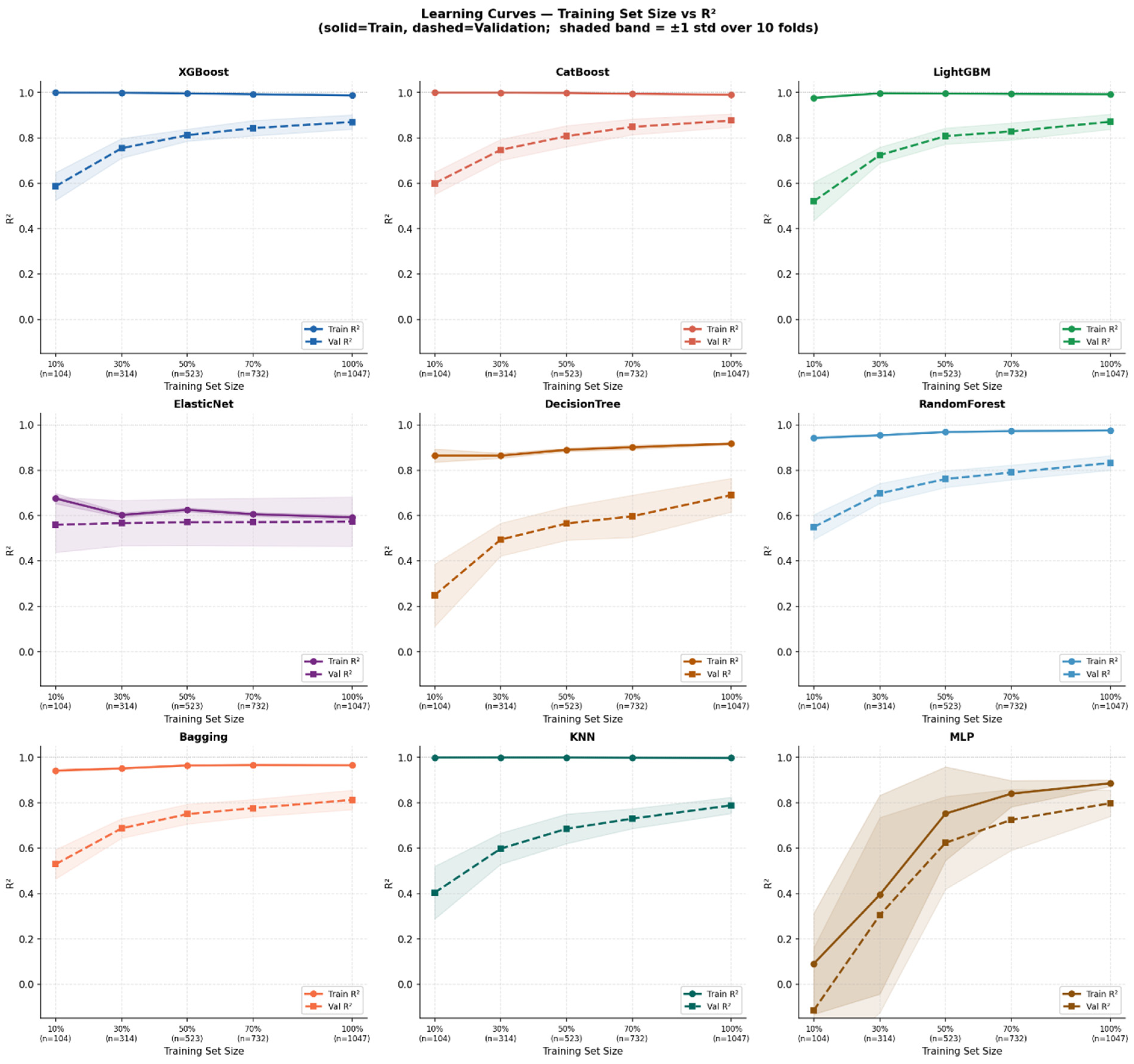
To assess whether each model genuinely learns from data or merely memorizes training patterns, learning curves were constructed by progressively increasing the training set size from 10% to 100% of the available training data (in five steps: 10%, 30%, 50%, 70%, and 100%), with train and validation R² recorded at each step via 10-fold cross-validation. A well-generalizing model exhibits a characteristic pattern: training R² decreases (i.e., can be a slight decrease) as more samples are added (reduced memorization), while validation R² increases and the two curves converge toward a common plateau, indicating that additional data reduces the bias–variance gap. In contrast, a high-variance (overfitting) model maintains near-perfect training R² across all sizes (with no decrease) while validation R² plateaus at a significantly lower level, with a persistent gap between the two curves.

3. Results

3.1. Model Training with Nested CV and Bayesian Hyperparameter Optimization

In the training stage, as explained earlier, the best (optimized) hyperparameters were derived from last outer fold.

Table 5. Optimized Hyperparameters.

Model	Optimized Hyperparameter Values
XGBoost	{‘n_estimators’: 507, ‘learning_rate’: 0.0835, ‘max_depth’: 4, ‘subsample’: 0.6675, ‘colsample_bytree’: 0.7838}
CatBoost	{‘iterations’: 703, ‘learning_rate’: 0.1686, ‘depth’: 5}
LightGBM	{‘n_estimators’: 642, ‘learning_rate’: 0.0873, ‘max_depth’: 9, ‘subsample’: 0.9098, ‘colsample_bytree’: 0.6368}
ElasticNet	{‘alpha’: 0.0203, ‘l1_ratio’: 0.9966}
DecisionTree	{‘max_depth’: 14, ‘min_samples_leaf’: 4}
RandomForest	{‘n_estimators’: 236, ‘max_features’: 0.7}
Bagging	{‘n_estimators’: 241, ‘base_max_depth’: 12}
KNN	{‘n_neighbors’: 4, ‘weights’: ‘distance’}
MLP	{‘hidden_layer_sizes’: (214, 241, 245), ‘activation’: ‘relu’, ‘learning_rate_init’: 0.0003513}

below presents the best hyperparameters identified for each model.

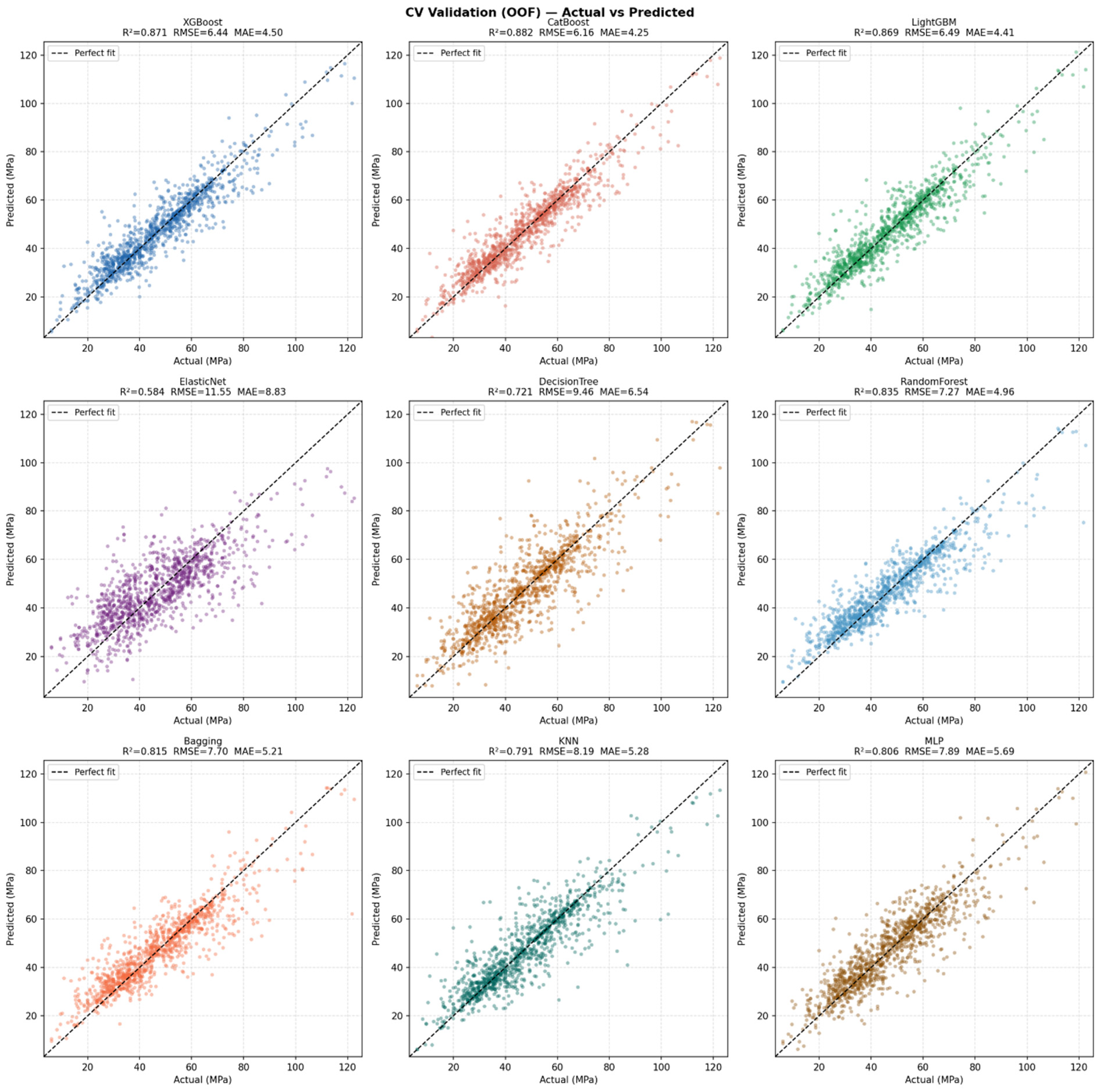
The results of the model training and evaluation process with nested cross-validation and Bayesian hyperparameter optimization are provided in

Table 6. Evaluation Metrics of ML Models (Nested CV Outer Folds and Holdout Set).

Model	CV Train R2	CV Train RMSE	CV Val R2	CV Val RMSE	Holdout R2	Holdout RMSE
XGBoost	0.9896	1.7714	0.8666	6.4151	0.8398	7.0867
CatBoost	0.9904	1.7136	0.8792	6.1367	0.8367	7.1555
LightGBM	0.9900	1.7629	0.8651	6.4602	0.8239	7.4300
Elastic Net	0.5922	11.4351	0.5738	11.5121	0.5977	11.2312
Decision Tree	0.9089	5.1679	0.7146	9.4299	0.7156	9.4424
Random Forest	0.9757	2.7912	0.833	7.2394	0.8121	7.6756
Bagging	0.9653	3.3377	0.8125	7.6525	0.7975	7.9679
KNN	0.9979	0.8229	0.7894	8.1578	0.7523	8.8132
MLP	0.8998	5.6406	0.8019	7.8535	0.7791	8.3224

. The CV Train, and CV Val metrics were obtained from the outer folds as mean values of all folds of Nested CV. The CV Val scores represent the results from data not seen for that fold by the hyperparameter optimizer, which is running on the inner folds. The holdout metrics were obtained from the holdout subset never seen during the training process.

Within the nested cross-validation framework employed in this study, the outer training and outer validation performances serve fundamentally different roles in assessing model behavior. The outer training performance reflects the model’s ability to fit the data used for parameter estimation after hyperparameter optimization has already been completed in the inner loop. In contrast, the outer validation performance represents a strictly unbiased estimate of predictive capability, as these validation folds remained completely unseen during both model training and hyperparameter tuning. Because hyperparameters were optimized exclusively using the inner cross-validation procedure applied to the outer training subset, the outer validation folds were fully isolated from the optimization process. Consequently, the performance measured on the outer validation folds provides a realistic simulation of model behavior on new, unseen data during the training process. The higher performance observed on the outer training subsets compared to the outer validation subsets is therefore expected and reflects the natural consequence of model fitting, rather than methodological bias or information leakage.

In the present results, models such as XGBoost, CatBoost, and LightGBM achieved very high outer training R² values, approaching 0.99 due to models’ capacity optimization with alignment to the data in that fold with hyperparameter tuning, while their outer validation R² values remained consistently high, ranging approximately between 0.86 and 0.88. This difference arises because the outer training subsets are directly used to estimate model parameters, allowing the model to more closely align with the specific structure of those data. In contrast, the outer validation subsets represent entirely independent samples that were not involved in either hyperparameter selection or parameter estimation.

The fact that validation performance remained consistently high despite this strict independence demonstrates that the models captured generalizable relationships rather than dataset-specific or fold-specific artifacts. A similar pattern was observed for ensemble models such as Random Forest and Bagging, which exhibited strong training performance accompanied by only moderate reductions in outer validation performance. This behavior confirms the effectiveness of ensemble learning in balancing model flexibility and generalization.

Conversely, simpler models such as Elastic Net showed smaller differences between training and validation performance, reflecting their more constrained functional form and lower capacity to fit complex patterns. Importantly, the nested cross-validation design used in this study eliminates optimistic bias because hyperparameter tuning, model fitting, and performance evaluation were performed on strictly separated data partitions. Therefore, the observed differences between outer training and outer validation performance represent the true and expected generalization gap inherent to supervised learning, rather than an artifact of improper evaluation.

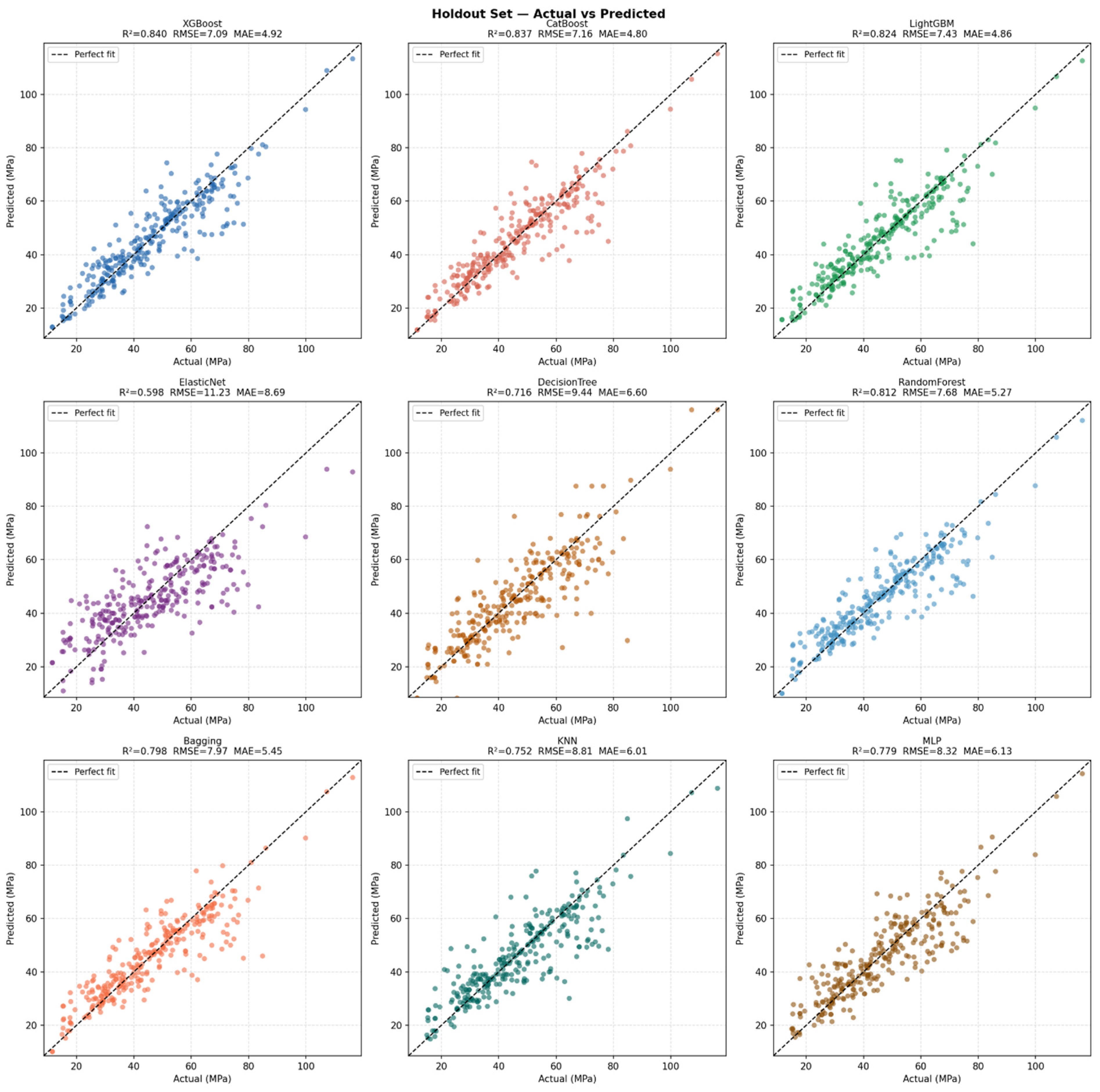
Figure 7 and Figure 8 show the predicted vs. true diagrams for validation holds and holdout subset. A critical indicator of model generalization is the degree of agreement between cross-validation performance and independent holdout performance.

In this study, the comparison of CV Validation R² and Holdout R² values across all models revealed a consistent and interpretable pattern. Among the gradient boosting models, XGBoost achieved a CV Validation R² of 0.8666 and a Holdout R² of 0.8398. It has a small difference of 0.0268. Similarly, CatBoost produced a CV Validation R² of 0.8792 and a Holdout R² of 0.8367 with a difference of 0.0425.

LightGBM showed a CV Validation R² of 0.8651 and Holdout R² of 0.8239. This yields a difference of 0.0412. These relatively small reductions indicate that the validation performance estimates were realistic and did not substantially overestimate model performance on unseen data.

The ensemble tree-based models demonstrated comparable behavior. Random Forest yielded CV Validation R² of 0.8330 and Holdout R² of 0.8121 (difference: 0.0209), while Bagging produced CV Validation R² of 0.8125 and Holdout R² of 0.7975 (difference: 0.0150). These minimal differences suggest highly stable generalization performance and confirm the robustness of ensemble methods in this dataset.

The Decision Tree model showed nearly identical performance between validation and holdout datasets with CV Validation R² of 0.7146 and Holdout R² of 0.7156, indicating virtually perfect agreement. This reflects low variance behavior but also confirms its comparatively limited predictive capacity relative to ensemble methods.

The neural network model (MLP) demonstrated moderate consistency with CV Validation R² of 0.8019 and Holdout R² of 0.7791 (difference: 0.0228). It is an acceptable generalization without substantial overfitting.

The K-Nearest Neighbors model exhibited the largest reduction, with CV Validation R² of 0.7894 and Holdout R² of 0.7523 (difference: 0.0371), suggesting relatively higher sensitivity to data variation and a slightly optimistic cross-validation estimate. Finally, Elastic Net regression showed an unusual but favorable pattern, where Holdout R² (0.5977) slightly exceeded CV Validation R² (0.5738). This indicates that cross-validation provided a conservative estimate of model performance rather than an optimistic one.

Overall, the differences between CV Validation R² and Holdout R² remained consistently small across all models, generally within the range of 0.01 to 0.04. Such close agreement confirms that the cross-validation procedure provided reliable and unbiased performance estimates. More importantly, the absence of large performance drops between validation and holdout datasets indicates that the models successfully learned generalizable relationships rather than memorizing the training data. Among all methods, gradient boosting and ensemble tree models demonstrated the best balance between predictive accuracy and generalization stability, confirming their suitability for this regression problem.

The CatBoost appeared as the best model based on the CV Validation R²/RMSE, but based on the Holdout R²/RMSE the XGBoost exhibited a slightly better performance. As the holdout performance is on an unseen data subset, we consider fine-tuned XGBoost as the best-performing model for this dataset.

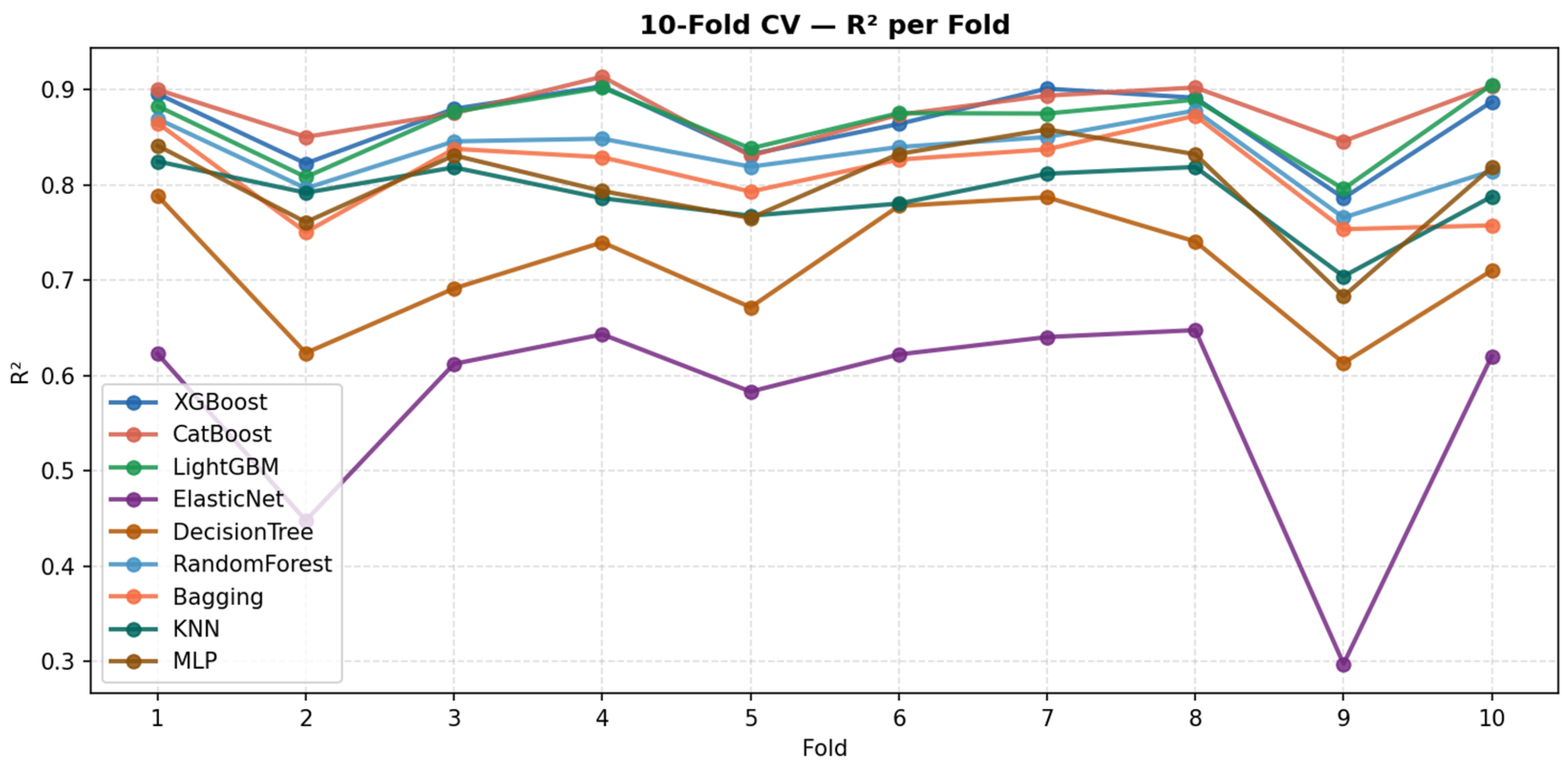
Figure 9 illustrates the CV Validation R² for each Outer Validation Fold of Train Subset. In folds 2 and especially 9, the models struggle to reach high metrics, and models exhibit a slight drop of performance in fold 5. The sharp decrease observed in fold 9 may be attributed to the presence of more complex validation samples or potential outliers within that fold. Other fold scores follow a flat line pattern, indicating that the model generalizes consistently in the remaining 7 folds.

3.2. Feature Importances and Model Interpretation

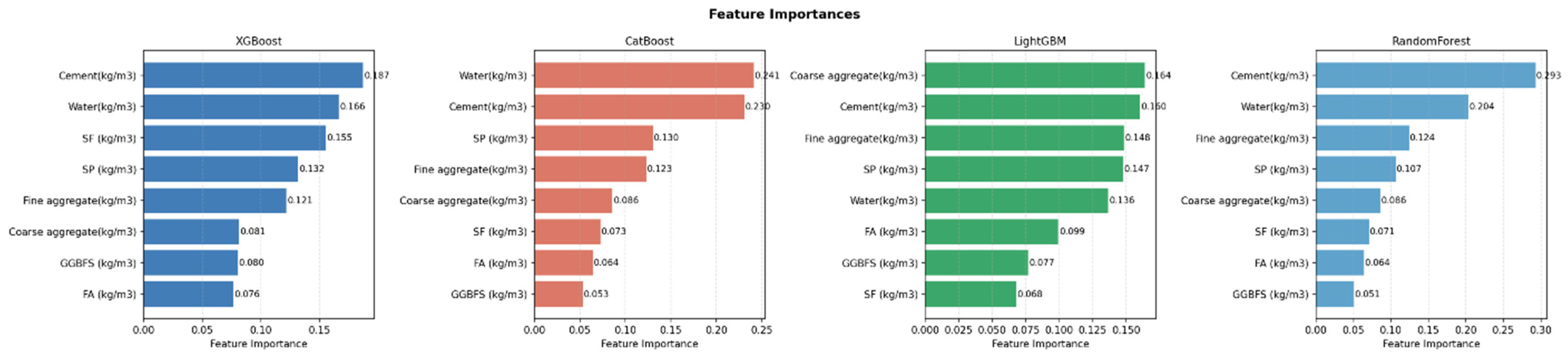
The comparative analysis of feature importance across XGBoost, CatBoost, LightGBM, and Random Forest models (Figure 10) revealed a highly consistent pattern in identifying the dominant factors governing the compressive strength of concrete containing SCMs, while also highlighting subtle model-specific differences in feature prioritization. Across three of four models, cement content and water content were consistently identified as the two most influential predictors, confirming their fundamental role in controlling concrete strength. In particular, Random Forest assigned the highest relative importance to the concrete mix proportion of cement (0.293), followed by water (0.204), while CatBoost similarly emphasized water (0.241) and cement (0.230) as the primary governing variables. XGBoost also demonstrated comparable trends, with cement and water ranked among the top predictors. This strong consensus across different algorithmic architectures confirms the dominant influence of binder quantity and water-to-binder ratio on compressive strength development.

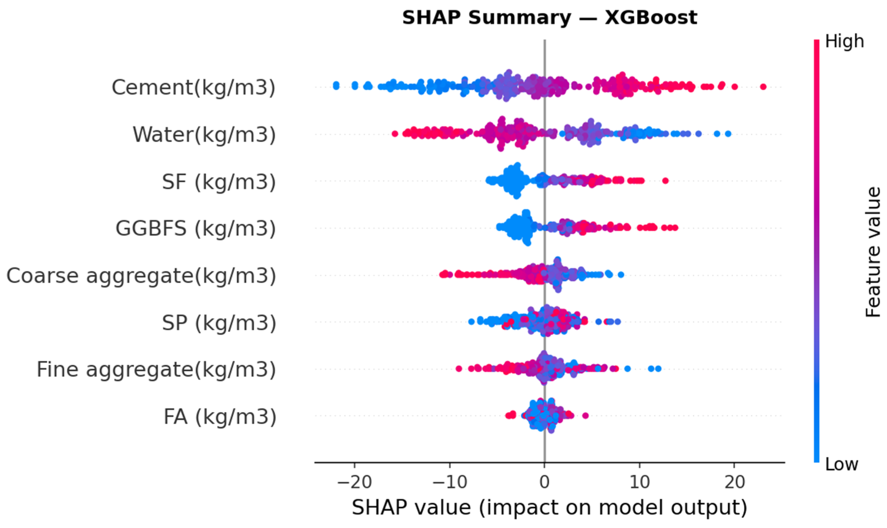
The feature importance rankings obtained using the XGBoost internal importance metric and SHAP analysis (Figure 11) showed some minor differences due to their fundamentally different computational principles. The XGBoost importance metric reflects the contribution of each feature to reducing the loss function in the tree-building process, while the SHAP importance represents the average magnitude of each feature’s contribution to the model’s prediction output. Therefore, some features, such as GGBFS, showed relatively lower importance in the tree-based importance metric but higher importance in the SHAP analysis. This indicates that GGBFS, although used less frequently in tree splitting, has a significant impact on the prediction results when used. In contrast, features such as SP and fine aggregate, although used more frequently in tree splitting, have a relatively lower overall impact on the prediction magnitude. These findings demonstrate that the SHAP method interprets feature impact more comprehensively and reliably because it directly quantifies the contribution of each feature to the model predictions rather than relying solely on the tree structure [46].

The SHAP summary analysis revealed that the most important parameter affecting compressive strength estimation was cement content, with higher cement amounts positively contributing to strength improvement. In contrast, water content showed an inverse relationship, with increasing water content negatively impacting the predicted strength. Complementary cementitious materials, particularly silica fume (SF) and GGBFS, showed positive effects at high dosages, confirming their beneficial role in increasing concrete strength. Aggregate-related variables and superplasticizer (SP) showed moderate effects, while the effect of fly ash (FA) remained relatively limited. This observation may be related to the characteristics of the dataset, since the influence of fly ash on compressive strength strongly depends on curing conditions and age. In particular, insufficient curing of fly ash-based concrete can significantly reduce compressive strength due to the slower pozzolanic reaction of FA compared to Portland cement. Higher aggregate amounts were generally associated with slightly negative or neutral SHAP values. High aggregate contents resulted in a decrease in estimated compressive strength, reflecting a dilution of the binder content in the mix. On the other hand, high SP content was more frequently associated with positive contributions, demonstrating its role in indirectly increasing strength by improving workability and particle packing. While high FA values sometimes provided positive contributions, their overall effect remained limited compared to other complementary cementitious materials. Overall, the SHAP analysis confirms that the model successfully captures the fundamental physical mechanisms determining concrete strength.

3.3. Permutation Significance Test

The permutation test results (

Table 7. Permutation Significance Test Results.

Model	Real Hold R2	Perm R2 Mean	Perm R2 Std	Perm R2 Max	p-Value	Significant
XGBoost	0.8398	−0.3403	0.1095	−0.1676	<<0.0001	Yes
CatBoost	0.8367	−0.307	0.1075	−0.0503	<<0.0001	Yes
LightGBM	0.8239	−0.4696	0.1137	−0.1622	<<0.0001	Yes
Elastic Net	0.5977	−0.0089	0.0443	0.1017	<<0.0001	Yes
Decision Tree	0.7156	−0.4616	0.1242	−0.1618	<<0.0001	Yes
Random Forest	0.8121	−0.2071	0.0767	−0.0286	<<0.0001	Yes
Bagging	0.7975	−0.116	0.0713	0.0633	<<0.0001	Yes
KNN	0.7523	−0.4162	0.0932	−0.1786	<<0.0001	Yes
MLP	0.7791	−0.1023	0.0686	0.08	<<0.0001	Yes

) confirmed that all machine learning models learned statistically significant relationships and did not simply memorize noise. Model performance decreased significantly when the target variable was replaced with a random permutation, with R² values dropping to negative values in the permuted models, compared to approximately 0.84 in the original models. This significant performance decrease indicates that the models’ predictive ability is entirely based on the actual relationships between the input variables and compressive strength. Furthermore, the permutation test produced a p-value of 0.0 for all models, confirming that the observed performance is statistically significant and not dependent on random chance. These findings provide strong evidence that the models perform genuine learning without overfitting.

3.4. Learning Curve Analysis

The learning curve analysis of all machine learning models (Figure 12) revealed consistent and robust generalization behavior. Validation performance steadily increased as the training set size increased, approaching a plateau level at larger sample sizes. Boosting models like XGBoost, CatBoost, and LightGBM have demonstrated near-perfect training and high validation performance, with the difference between training and validation curves decreasing as the dataset increases, showing strong learning capacity without severe overfitting. Similarly, ensemble methods like Random Forest and Bagging have shown learning behavior where validation performance increases steadily, and a moderate, controlled difference is maintained relative to training performance. This confirms a well-balanced bias–variance trade-off.

Decision Tree and KNN models started with a larger training–validation difference at smaller sample sizes, reflecting high variance and sensitivity to limited data; however, this difference decreased significantly as the dataset increased, and generalization ability improved. The MLP model showed a significant improvement in both training and validation performance as the dataset size increased, demonstrating that sufficient data is necessary for the neural network to effectively learn fundamental relationships. In contrast, the ElasticNet model showed poor performance with training and validation curves almost overlapping, experiencing underfitting due to limited model complexity, not overfitting. It is important to note that the convergence of the validation curves in all models and the decrease in performance variance over larger training sets indicate that the dataset is large enough to capture the underlying predictive relationships.

Overall, these findings confirm that the advanced ensemble and boosting models achieved the best generalization performance while maintaining robustness and avoiding overfitting, whereas simpler models were primarily limited by underfitting rather than excessive variance.

4. Conclusions

We provided a robust machine learning-based framework for estimating the compressive strength of SCM-blended concrete on a comprehensive global dataset of concrete mixtures containing cement-based materials. Considering that the cement industry contributes greatly to CO₂ emissions, increasing the use of SCM such as fly ash, silica fume, high furnace slag, and natural light stone is not only an environmental necessity but also a means to improve the long-term properties of concrete.

In this study, a new pipeline including a nested cross-validation framework combined with Bayesian hyperparameter optimization was implemented to ensure the optimal performance of each model can be determined and evaluated for this dataset. Furthermore, the framework included a permutation significance testing and Learning Curve Analysis to ensure that the models evaluated learned genuine relationships rather than random patterns. The comparison between cross-validation and independent holdout performance, together with learning curve analysis, was used to confirm the absence of overfitting and to demonstrate that the models achieved true generalization. Finally, SHAP-based explainable artificial intelligence was utilized to interpret the influence of individual mixture components on strength prediction.

The most highly performing models include XGBoost, which achieved a CV validation R² of 0.8666 and a holdout R² of 0.8398, followed by CatBoost and LightGBM with very similar performance metrics. The small differences observed between XGBoost and CatBoost indicate that both models demonstrated similarly strong predictive performance, while XGBoost showed a slight advantage (0.8398 vs. 0.8367 R²) on the holdout dataset, this difference may depend on the specific data split and does not necessarily indicate that there exists a universally superior model.

The results suggest that ensemble machine learning models are highly effective in capturing the underlying patterns in the dataset and accurately predicting the compressive strength of SCM concrete.

In addition, the SHAP analysis revealed that cement content was the most influential parameter, showing a positive relationship with compressive strength. Water content was identified as the second-most influential variable, exhibiting an inverse relationship. SCMs, particularly silica fume (SF) and GGBFS, showed positive contributions at higher dosages, confirming their beneficial role in enhancing concrete strength.

The main limitation of this study is that the models were developed using a global dataset containing only mixture composition variables, without incorporating external factors such as curing conditions, temperature, and humidity, which may influence concrete strength and limit generalizability under different field conditions. These factors will be tested with a new dataset in our feature research. In addition, future research will not only focus on the 28-day intensity, but also on the development of an interpretation model that can predict the intensity of the expression curve.