Article

Multi-Strategy-Enhanced Improved Horned Lizard Optimization Algorithm for Path Planning in Mobile Robots

1
School of Mathematics and Information Engineering, Lianyungang Normal University, Lianyungang 222006, China
2
Institute of Functional Materials and Applied Technology, Lianyungang Normal University, Lianyungang 222006, China
3
School of Information and Control Engineering, China University of Mining and Technology, Xuzhou 221116, China
*
Author to whom correspondence should be addressed.
Algorithms 2026, 19(4), 272; https://doi.org/10.3390/a19040272
Submission received: 9 February 2026 / Revised: 20 March 2026 / Accepted: 27 March 2026 / Published: 1 April 2026

Abstract

Aiming at the inherent defects of the Horned Lizard Optimization Algorithm (HLOA), such as insufficient global exploration capability, premature convergence to local optima, and inadequate balance between exploration and exploitation, this paper proposes an enhanced Improved Horned Lizard Optimization Algorithm (IHLOA) integrated with multi-strategy improvements. Firstly, the Fuch chaotic mapping is introduced for population initialization, which enhances the ergodicity and diversity of the initial population by leveraging the pseudo-random and aperiodic characteristics of chaotic sequences, laying a high-quality foundation for subsequent optimization searches. Secondly, the golden sine strategy is embedded into the iterative update process to dynamically adjust the search step size and direction. This strategy utilizes the periodic amplitude variation in the sine function and the golden section coefficient to balance the global exploration for potential optimal regions and local exploitation for refined optimization, thereby accelerating convergence speed while avoiding local stagnation. Finally, the orthogonal crossover strategy is incorporated in the late iteration stage to promote effective information interaction between parent and offspring populations. By means of chromosome segment exchange and elitist retention mechanisms, this strategy reduces dimensional search blind spots and further enhances the algorithm’s ability to capture high-quality solutions. Comprehensive experimental evaluations are conducted based on classical benchmark test functions and eight state-of-the-art meta-heuristic algorithms. The results demonstrate that the IHLOA outperforms comparative algorithms in terms of optimization accuracy, convergence speed, and stability across 30-D, 50-D, and 80-D scenarios. For practical path planning applications, the IHLOA achieves remarkable performance improvements: in single-goal path planning, it reduces the path length by 2.54–87.64% compared with benchmark algorithms; in multi-goal path planning, it realizes a 1.24–7.99% reduction in path length and an 11.91% average reduction in the number of turning points relative to the original HLOA. Additionally, the IHLOA exhibits excellent robustness and adaptability in dynamic obstacle environments, effectively shortening the path length and reducing robot stuck times. This research not only enriches the improvement framework of meta-heuristic algorithms but also provides a high-efficiency optimization solution for mobile robot path planning in complex environments.

1. Introduction

In recent years, the field of mobile robots has undergone rapid innovation towards intelligence. As a typical paradigm of multidisciplinary integration, the development trajectory of modern mobile robot path planning technology has always been deeply coupled with the iterative upgrading of mobile robot technology [1,2]. The core of this technology lies in enabling mobile robots to safely, robustly, efficiently, and accurately execute tasks in diverse and complex environments. Specifically, it is necessary to construct a path optimization model by comprehensively considering multiple dimensions such as system operational dynamics and environmental constraints. In this process, performance parameters such as path smoothness and the energy consumption ratio of travel distance constitute the core evaluation index system for measuring the quality of path planning schemes [3,4].
Classical path-searching algorithms such as the A* algorithm, Rapidly-exploring Random Tree (RRT) algorithm, and Artificial Potential Field (APF) algorithm have established a broad application foundation in the field of mobile robot path planning. Among them, Nhouchi et al. [5] proposed a real-time A* algorithm framework for uncertain environments, which was successfully applied to automated assembly task scenarios through the collaborative design of dynamic trajectory generation and collision avoidance mechanisms. Aiming at the optimization efficiency bottleneck of the single A* algorithm in complex topological spaces, Jin et al. [6] developed a hybrid improvement strategy, effectively addressing the inefficiency of traditional algorithms in searching for optimal paths under multi-constraint conditions. In the optimization of the RRT algorithm system, Liang et al. [7] proposed an improved RRT algorithm integrating an adaptive sampling strategy and a path optimization mechanism. Through dynamic adjustment of sampling density and curvature optimization iteration, the path smoothness index was significantly improved. Aiming at the autonomous navigation requirements of robots in complex orchard environments, Cao et al. [8] constructed a collaborative framework of the improved LeGO-LOAM algorithm and the RRT algorithm, achieving high-precision path planning for robots between fruit tree rows through refined environmental map construction and dynamic path correction. Shen et al. [9] proposed a fusion model of RRT and Dijkstra algorithms, synchronously enhancing path planning efficiency and smoothness performance through the complementary advantages of heuristic search and graph theory optimization. Additionally, Wu et al. [10] introduced a farthest point optimization strategy to increase path diversity and help avoid local optimal solutions.
With the continuous development of computational intelligence and big data technologies, the breadth and depth of applications of swarm intelligence optimization algorithms have significantly expanded across multiple domains. Typical algorithms include Ant Colony Optimization (ACO), Particle Swarm Optimization (PSO), Sparrow Search Algorithm (SSA), Grey Wolf Optimizer (GWO), Whale Optimization Algorithm (WOA), and Crested Porcupine Optimizer (CPO), among others. Cui et al. [11] proposed a direction-guiding mechanism that steers ants to preferentially select certain directions during the search process, thereby enhancing the algorithm’s exploration efficiency and the likelihood of discovering superior paths. Hu et al. [12] incorporated the concept of coevolution by dividing particle swarms into multiple subgroups, each optimized for distinct tasks or objectives, which significantly improved algorithmic diversity and search efficiency. Mishra et al. [13] addressed the challenges of reducing memory requirements, avoiding local optima, and enhancing algorithm efficiency by integrating the advantages of Particle Swarm Optimization (PSO) and Artificial Potential Field (APF) methods. Wang et al. [14] proposed an improved Sparrow Search Algorithm (SSA), optimizing its performance through multi-strategy fusion to tackle complex optimization problems. Xu et al. [15] enhanced the exploration and exploitation capabilities of the sparrow algorithm by refining the position update strategies for producers and followers. Qu et al. [16] improved the path planning capability of unmanned combat aerial vehicles in complex environments by modifying SSA and integrating a dual-layer encoding mechanism. Inspired by the hunting behavior of black-winged kites, Wang et al. [17] developed a novel nature-inspired optimization algorithm, the Black-Winged Kite Algorithm (BKA), aimed at enhancing global search capability and convergence efficiency. Mohamed et al. [18] proposed the Crested Porcupine Optimizer (CPO), a new nature-inspired optimization algorithm mimicking the defense, foraging, and group collaboration behaviors of crested porcupines to improve the algorithm’s global search capability and robustness. Inspired by tribal competition and member collaboration behaviors, Chen et al. [19] introduced the Competition and Tribal Collaboration with Members (CTCM) algorithm, which resolves the contradiction between exploration and exploitation in traditional algorithms through a dynamic balance mechanism of competition and collaboration.
The Horned Lizard Optimization Algorithm (HLOA), proposed by Pérez et al. [20], is a nature-inspired meta-heuristic algorithm whose theoretical framework is derived from the multi-layered defensive behaviors of horned lizards against predators—including blood-squirting deterrence, crypsis (environmental camouflage), and body inflation for defense. This algorithm constructs a dynamic search model suitable for complex optimization problems by abstracting biological defense mechanisms into neighborhood perturbation, adaptive sampling, and local extremum avoidance strategies in the search space. Experimental results demonstrate that the HLOA exhibits significant advantages in scenarios such as high-dimensional space optimization and dynamic constraint solving, effectively converging to high-quality approximate solutions. Through multi-metric comparisons with classical algorithms like PSO (Particle Swarm Optimization) and GWO (Grey Wolf Optimizer)—such as convergence speed, solution accuracy, and stability—its competitiveness in complex optimization tasks is validated. In practical applications, the HLOA has been successfully applied to multi-UAV collaborative monitoring path planning in disaster scenarios. By constructing a multi-objective optimization model that integrates obstacle avoidance, travel distance minimization, and monitoring coverage maximization, the algorithm dynamically generates three-dimensional path solution sets adapted to debris environments, providing real-time path decision support for emergency rescue command. However, the algorithm still faces prominent limitations that restrict its application in complex path planning scenarios: (1) the random initialization method leads to uneven distribution of the initial population, resulting in insufficient ergodicity and limiting the global search potential of the algorithm; (2) the position update mechanism lacks adaptive adjustment of search step size and direction, leading to rapid attenuation of population diversity during iteration and proneness to premature convergence to local optima; (3) the lack of effective information interaction mechanisms between individuals results in search blind spots in the late iteration stage, reducing the ability to capture high-quality solutions.
To address the aforementioned research gaps in existing optimization algorithms, this paper proposes an Enhanced Improved Horned Lizard Optimization Algorithm (IHLOA) by constructing a multi-layered improvement framework. During the population initialization phase, the Fuch chaotic mapping is introduced to replace traditional random generation methods. By leveraging the aperiodic ergodic property of chaotic sequences, this approach enhances the distribution uniformity of the initial population in the search space, effectively mitigating the population aggregation bias caused by conventional initialization methods. In the iterative optimization process, a golden sine strategy is incorporated to dynamically adjust the search step size. This strategy utilizes the periodic amplitude variation in the sine function to synergistically optimize the algorithm’s global exploration and local exploitation capabilities: larger amplitudes are employed in the early search stage to expand the solution space and reduce the risk of premature convergence; in the late search stage, amplitude decay is used to achieve fine-grained optimization in local regions, balancing the dual objectives of maintaining population diversity and improving convergence efficiency. In the late search stage, an orthogonal crossover operator is introduced, generating offspring individuals through a chromosome segment exchange mechanism via pairwise pairing of individuals. Specifically, after performing fitness-based sorting of the population, crossover operations are executed, and an elitist retention strategy is adopted to update the population by comparing the fitness values of offspring and parent individuals. This mechanism enhances genetic diversity, reduces search blind spots, effectively suppresses local optimum stagnation in late iterations, and strengthens the capability to capture high-quality solutions.
The main contributions of this study are summarized as follows:
(1)
Propose a multi-strategy enhanced IHLOA to address the core defects of the HLOA (uneven initial population distribution, weak balance between exploration and exploitation, insufficient information interaction, and high parameter sensitivity), providing a novel and efficient optimization framework for meta-heuristic algorithms.
(2)
Integrate Fuch chaotic mapping, the golden sine strategy, and the orthogonal crossover strategy into the HLOA framework and clarify the synergistic optimization mechanism of each strategy for improving population diversity, convergence speed, and the ability to obtain high-quality solutions through theoretical analysis and ablation experiments.
(3)
Conduct comprehensive comparative experiments on benchmark test functions (30-D, 50-D, 80-D) and path planning scenarios (single-goal, multi-goal, dynamic environment) to systematically verify the superiority of the IHLOA over existing classical algorithms in terms of optimization accuracy, robustness, high-dimensional scalability, and practical application effect.
(4)
Provide an optimized solution for mobile robot path planning that can potentially improve path quality and reduce motion control costs: by enhancing the algorithm’s optimization capability, the planned path is expected to be shorter and smoother, thereby lowering the energy consumption of robots in actual navigation and improving their adaptability to complex environments.

2. Methods

2.1. Horned Lizard Optimization Algorithm (HLOA)

The horned lizard has evolved unique survival strategies, including hormone-regulated color changing, body temperature control via skin lightening/darkening, blood-squirting defense, and rapid escape behavior. These strategies inspire the mathematical modeling of a meta-heuristic algorithm as follows:

2.1.1. Crypsis Color Change Strategy

The horned lizard achieves environmental camouflage by dynamically adjusting skin color. In the CIE Lab color space, L* represents lightness, and a* (red–green axis) and b* (blue–yellow axis) denote chromatic coordinates. In the LCh space, L* is lightness, C* is chroma, and h* is the hue angle (0–360°). The color transformation is modeled as:
c o l o r V a r = c 1 sin h p cos h q ± c 2 sin h r cos h s
where hp, hq, hr, and hs are distinct hue angles, and c 1 c 2 are random chroma values from a normalized color palette. The search update equation guided by the optimal solution is:
x i t + 1 = x b e s t t + t M a x _ i t e r c 1 sin x r 1 t cos x r 2 t 1 σ c 2 cos x r 3 t sin x r 4 t
Here, x i t + 1 is the new search position in the (t + 1)-th generation, x b e s t t is the current best solution, the x r k t (k = 1, 2, 3, 4) represent the position vectors of four distinct randomly selected individuals at iteration t, M a x _ i t e r is the maximum number of iterations, σ is generated by a random strategy within [0, 1], and = 2 , and c 1 , c 2 are sampled from the normalized color palette.

2.1.2. Skin Lightening/Darkening Strategy

The horned lizard regulates solar heat absorption through skin color, modeled by Equation (3) for lightening (cooling) and (4) for darkening (heating):
x w o r s t t = x b e s t t + 1 2 L i g h t 1 sin x r 1 t x r 2 t 1 σ 1 2 L i g h t 2 sin x r 3 t x r 4 t
x w o r s t t = x b e s t t + 1 2 D a r k 1 sin x r 1 t x r 2 t 1 σ 1 2 D a r k 2 sin x r 3 t x r 4 t
L i g h t 1 , L i g h t 2 0 , 0.4046661 , D a r k 1 , D a r k 2 0.5440510 , 1 . x w o r s t t updates via random selection of lightening/darkening to maintain population diversity.

2.1.3. Blood-Squirting Defense Strategy

The blood-squirting behavior is modeled as a projectile motion, with horizontal uniform linear motion and vertical uniformly accelerated motion:
x i t + 1 = v 0 cos a t M a x _ i t e r + ε x b e s t t + v 0 sin a a t M a x _ i t e r g + ε x i t
where initial velocity v0 = 1 m/s, launch angle is α = π 2 , g is the gravitational acceleration, and perturbation is ε = 10 6 . This model enables efficient global exploration via ballistic trajectory simulation.

2.1.4. Move-to-Escape Strategy

Threat-induced rapid movement combines local perturbation and global displacement:
x i t + 1 = x b e s t t + walk 1 2 ε x i t
Here, walk is a random number from a Cauchy distribution (mean 0, standard deviation 1), and ε is a standard Cauchy sample. This strategy enhances local exploitation and global exploration via x b e s t t -guided displacement.

2.1.5. α-Melanophore-Stimulating Hormone (α-MSH) Rate Strategy

The skin color change of the horned lizard is regulated by the α-melanophore-stimulating hormone (α-MSH) rate, whose calculation formula is as follows:
m e l a n o p h o r e i = F i t n e s s max F i t n e s s i F i t n e s s max F i t n e s s min
Melanophore (i) is the α-MSH rate of the i-th search individual, normalized to the interval [0, 1]. When m e l a n o p h o r e i 0.3 , individual replacement is triggered:
x i t = x b e s t t + 1 2 x r 1 t 1 x r 2 t

2.2. Improved Horned Lizard Optimization Algorithm (IHLOA)

2.2.1. Fuch Chaotic Mapping

In the natural environment, the initial habitat distribution of the horned lizard has inherent ergodicity and spatial uniformity. Wild populations are evenly dispersed throughout the entire living domain to avoid food shortage and concentrated predation risk by natural enemies caused by population aggregation. This spatial distribution characteristic is the basis for the horned lizard population to maintain survival advantages in the wild environment. However, the random initialization method adopted by the original HLOA cannot simulate the uniform distribution characteristics of the horned lizard in its natural habitat, which easily leads to aggregation bias in the initial population and limits the initial global search advantage of the algorithm. In response to this, this paper introduces Fuch chaotic mapping to complete the optimization of the population initialization stage. Commonly used chaotic map models include the Logistic map, Henon map, Tent map, etc. Among them, the Fuch map, as a chaotic mapping with infinite folding characteristics, exhibits superior ergodicity performance, stronger dynamical characteristics, and better convergence performance. Through the aperiodicity, ergodicity and pseudo-randomness of the chaotic sequence, it can accurately simulate the uniform initial distribution characteristics of the horned lizard in the search space and construct an initial population with more comprehensive spatial coverage and better diversity for the algorithm at the initial stage of iteration. At the same time, the map can effectively improve the search efficiency and solution accuracy of the algorithm through continuous compression of the search area during the iteration process [21,22,23,24,25]. Its mathematical expression is shown in Equation (9):
X i + 1 = cos 1 X i 2
where X i 0 , i Z + .

2.2.2. Golden Sine Strategy

During the escape and foraging process of the horned lizard in the wild, it dynamically adjusts the moving step size and travel direction according to the real-time distance from itself to natural enemies and food sources. Its moving trajectory presents a typical sinusoidal periodic fluctuation characteristic. Through this variable-amplitude fluctuating movement mode, it can not only complete wide-area spatial exploration through large-scale movement in long-distance scenarios to avoid path prediction by natural enemies, but it can also achieve precise convergence to the target site through small-scale fine adjustment in short-distance scenarios. This adaptive movement behavior is the core for the horned lizard to balance survival risk and foraging efficiency in complex wild environments. However, the position update mechanism of the original HLOA does not carry out fine-grained modeling of this adaptive movement behavior of the horned lizard, which leads to the rapid attenuation of population diversity during the iteration process of the algorithm and then the premature convergence problem of falling into the local optimum. In view of this, this paper introduces the golden sine strategy into the iteration process of the HLOA to optimize the population position update mechanism of the algorithm. This strategy integrates the golden section coefficient with the periodic characteristics of the sine function and mathematically simulates the adaptive adjustment behavior of the step size during the movement of the horned lizard through the periodic variable amplitude characteristics of the sine function. In the early stage of iteration, large-amplitude sinusoidal fluctuation is adopted, corresponding to the wide-area exploration behavior of the horned lizard to expand the search space and reduce the risk of premature convergence. In the late stage of iteration, small-amplitude fine adjustment is used, corresponding to the precise convergence behavior of the horned lizard to the target site, to strengthen the local exploitation ability of the algorithm and finally realize the dynamic balance between global exploration and local exploitation of the algorithm [26,27,28]. The position update mechanism after introducing the golden sine strategy is shown in Equation (10):
x i t + 1 = x i t × sin r 1 r 2 × sin r 1 × x b e s t t x i t
where x i t is the position of the i-th individual at the t-th iteration, x i t + 1 is the position of the i-th individual at the (t + 1)-th iteration, x b e s t t is the current optimal position at the t-th iteration, and r1 and r2 are two random numbers within the interval 0 , 2 π .
Convergence Analysis:
The updated search agent position is bounded in the feasible solution space Ω . Specifically, since r 1 0 , 1 , we have sin ( r 1 ) 0 , 1 , and combined with r 2 0 , 2 π , the product term r 2 × sin ( r 1 ) satisfies r 2 × sin ( r 1 ) 2 π , 2 π ; as x b e s t , j t and x i , j t are both positions of search agents, they are inherently within the feasible solution space Ω , and the updated position x i , j t + 1 is a linear combination of these two variables with bounded coefficients, x i , j t + 1 Ω , proving the position is bounded.
The update formula converges: the sequence of search agent positions x i , j t is bounded within Ω ; the fitness function f(x) is continuous and bounded on the closed and bounded set Ω , so according to the Weierstrass Extreme Value Theorem, f(x) attains its minimum value f x on Ω and thus has a lower bound. In the iteration process, r1 adjusts the search direction via sin ( r 1 ) , and r2 modulates the step size through r 2 × sin ( r 1 ) × x b e s t , j t x i , j t , which drives x i , j t progressively closer to x b e s t , j t and ensures the fitness function value f x i , j t is monotonically non-increasing with iterations. By the Monotone Bounded Convergence Criterion, a monotonically non-increasing sequence bounded below must converge, so t , f x i , j t f x , where x denotes the high-quality optimal solution, confirming that the formula converges to the high-quality optimal solution.

2.2.3. Orthogonal Crossover Strategy

Horned lizards are not solitary creatures. In their natural habitat, individuals within the population complete real-time conveyance of survival information through visual signals, sharing the location information of safe habitats, high-quality food sources and enemy activity areas. Through information collaboration and experience sharing within the population, the survival probability of the entire population is improved. This cross-individual information interaction behavior within the population is the key for the horned lizard population to adapt to the complex wild environment. However, the original HLOA does not model this population collaborative behavior, and there is a lack of an effective information interaction mechanism in the individual iteration process, which leads to the individuals easily gathering in the local optimal area in the late iteration of the algorithm, resulting in search blind spots and thus reducing the global search efficiency of the algorithm. To address this issue, this paper introduces a crisscross orthogonal crossover strategy to simulate the information interaction behavior in the horned lizard population through mathematical modeling. This strategy expands the search space through cross-dimensional crossover operations to reduce search blind spots and improve the global optimization performance of the algorithm [29,30,31,32]. Among them, horizontal crossover, as an information exchange mechanism between individuals of the same generation, corresponds to the survival information-sharing behavior between contemporaneous individuals in the horned lizard population. By randomly pairing individuals in the population, offspring individuals are generated through parent crossover, and individuals with better fitness values are retained. Its mathematical formulas are shown in Equations (11) and (12):
M i , d k = e 1 × x i , d k + 1 e 1 × x j , d k + c 1 × x i , d k x j , d k
M j , d k = e 2 × x j , d k + 1 e 2 × x i , d k + c 2 × x j , d k x i , d k
where x i , d k and x j , d k denote the parent individuals in the d-th dimension, and M i , d k and M j , d k represent the offspring individuals generated via the crossover operation in the d-th dimension. e 1 and e 2 are random numbers in the interval [0, 1], while c 1 and c 2 are random numbers in the interval [−1, 1].
Vertical crossover, serving as an information interaction mechanism across dimensions, operates by pairing individuals from different dimensions in the population and generating offspring through crossover operations. Similar to horizontal crossover, offspring produced by vertical crossover undergo fitness competition with parent individuals, with higher-performing individuals retained. The mathematical formulation is as follows:
M i , d k = e × x i , d 1 k + 1 e × x i , d 2 k
where x i , d 1 k and x i , d 2 k denote the parent individuals in the d 1 -th and d 2 -th dimensions, respectively; M i , d k represents the offspring individual generated by crossover between the d 1 -th and d 2 -th dimensional parent individuals; and e is a random number in the interval [0, 1].

2.3. Flowchart of the Improved Horned Lizard Optimization Algorithm (IHLOA)

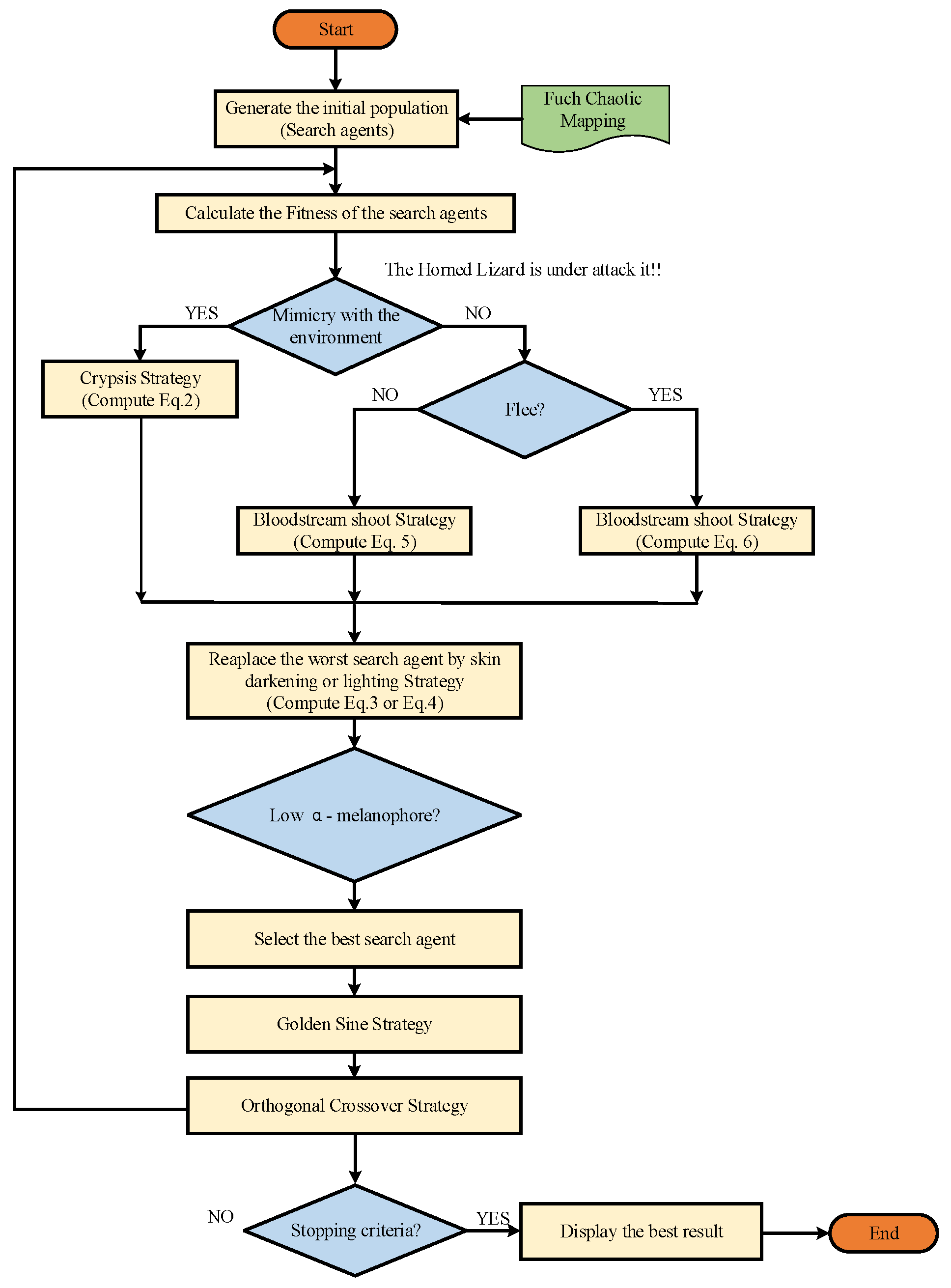
Based on the core bionic logic of the original HLOA, this paper proposes an improved Horned Lizard Optimization Algorithm (IHLOA). The algorithm retains the mathematical modeling of the four defense strategies (crypsis, skin lightening/darkening, blood-squirting, move-to-escape) and the α-melanophore-stimulating hormone (α-MSH) regulation mechanism of the horned lizard from the HLOA. Meanwhile, addressing the insufficient balance between exploration and exploitation in the original algorithm in high-dimensional optimization scenarios, the IHLOA incorporates three additional strategies, the chaotic initialization strategy, the golden sine strategy, and the orthogonal crossover strategy, further optimizing search efficiency and convergence performance. The flowchart is presented in Figure 1, clearly illustrating the complete process of population initialization, multi-strategy collaborative search, fitness evaluation, and optimal solution update.

2.4. Computational Complexity

Time complexity serves as a core metric for evaluating the solution efficiency and practical application value of an algorithm. Therefore, this section specifically conducts a time complexity analysis for the IHLOA. Let N represent the population size of the horned lizard, D denote the dimension of the optimization problem, T indicate the maximum number of iterations, and FE stand for the time complexity of a single fitness evaluation. Based on the design logic and code implementation of the original HLOA, the total time complexity of the original HLOA is O(T × N × (D + FE)), which belongs to the linear time complexity category.
Compared with the original HLOA, the IHLOA incorporates three additional strategies: chaotic initialization, the sine cosine strategy, and the crisscross crossover strategy. Firstly, in the initialization phase, the IHLOA replaces the original random initialization with population generation via chaotic mapping. At this point, the time complexity remains consistent with the original HLOA, still being O(N × (D + FE)). Secondly, during the iteration phase, the core position update logic of the original HLOA (including protective color mimicry, blood-squirting defense, escape wandering, skin light/dark regulation, and α-melanophore-stimulating hormone regulation) is retained. For each generation, this logic performs D-dimensional position updates and fitness evaluations for N individuals, with a time complexity of O(N × (D + FE)), which is identical to the original algorithm. Meanwhile, the sine cosine strategy and crisscross crossover mutation strategy introduced in the iteration only involve constant-time operations, independent of N and D, resulting in a time complexity of O(1) without additional complexity. Thirdly, at the end of each iteration, the sine cosine strategy is applied to perform position perturbations on N individuals, followed by a re-evaluation of fitness. The time complexity of correcting the perturbed positions and calculating the fitness once is O(N × (D + FE)). Additionally, the optimal vector sorting operation added in the algorithm only targets the D-dimensional optimal solution, with a time complexity of O(DlogD), which is a constant-level operation and does not alter the overall complexity order of the algorithm.
Consequently, the total time complexity of the IHLOA is O(2 × T × N × (D + FE)). This result indicates that the time complexity of the IHLOA only increases in coefficient compared to the HLOA, both having linear time complexity. The algorithm improvements do not introduce additional time complexity orders, thus avoiding order-level degradation in solution efficiency caused by algorithm modifications.

3. Results and Discussion

3.1. Sensitivity Analysis

To investigate the influence law of core parameters on the optimization performance of the proposed Improved Horned Lizard Optimization Algorithm (IHLOA) and determine the optimal parameter configuration, this section conducts a systematic sensitivity analysis on three core parameters introduced by the improved strategies: the sine control parameters r1 and r2 from the golden sine strategy and the crossover probability pc from the orthogonal crossover strategy.
The analysis is performed on 21 widely used classical benchmark test functions (see Table A1). Among them, F1–F7 are unimodal test functions, which are mainly adopted to test the convergence speed and local exploitation capability of the algorithms; F8–F13 are multimodal test functions, which are applied to evaluate the global exploration capability of the algorithms to escape from local optima; and F14–F21 are composite benchmark test functions, which are designed to verify the comprehensive solution performance of the algorithms in complex optimization scenarios and simulate the difficulty of practical engineering optimization problems. During the experiments, all other hyperparameters of the algorithm are fixed to eliminate confounding variables, while multiple gradient levels are set for each target parameter. Two quantitative metrics are employed for performance evaluation: the average optimal value (avg) obtained from independent repeated runs to characterize the optimization accuracy and the standard deviation (std) to quantify the stability and robustness of the optimization results. In addition, radar plots and average ranking plots are utilized to provide a holistic and quantitative comparison of the comprehensive performance across different parameter values, where a lower average ranking value corresponds to a superior overall ranking across the entire test suite, indicating better comprehensive algorithmic performance.

3.1.1. Sensitivity Analysis of Sine Parameter r1

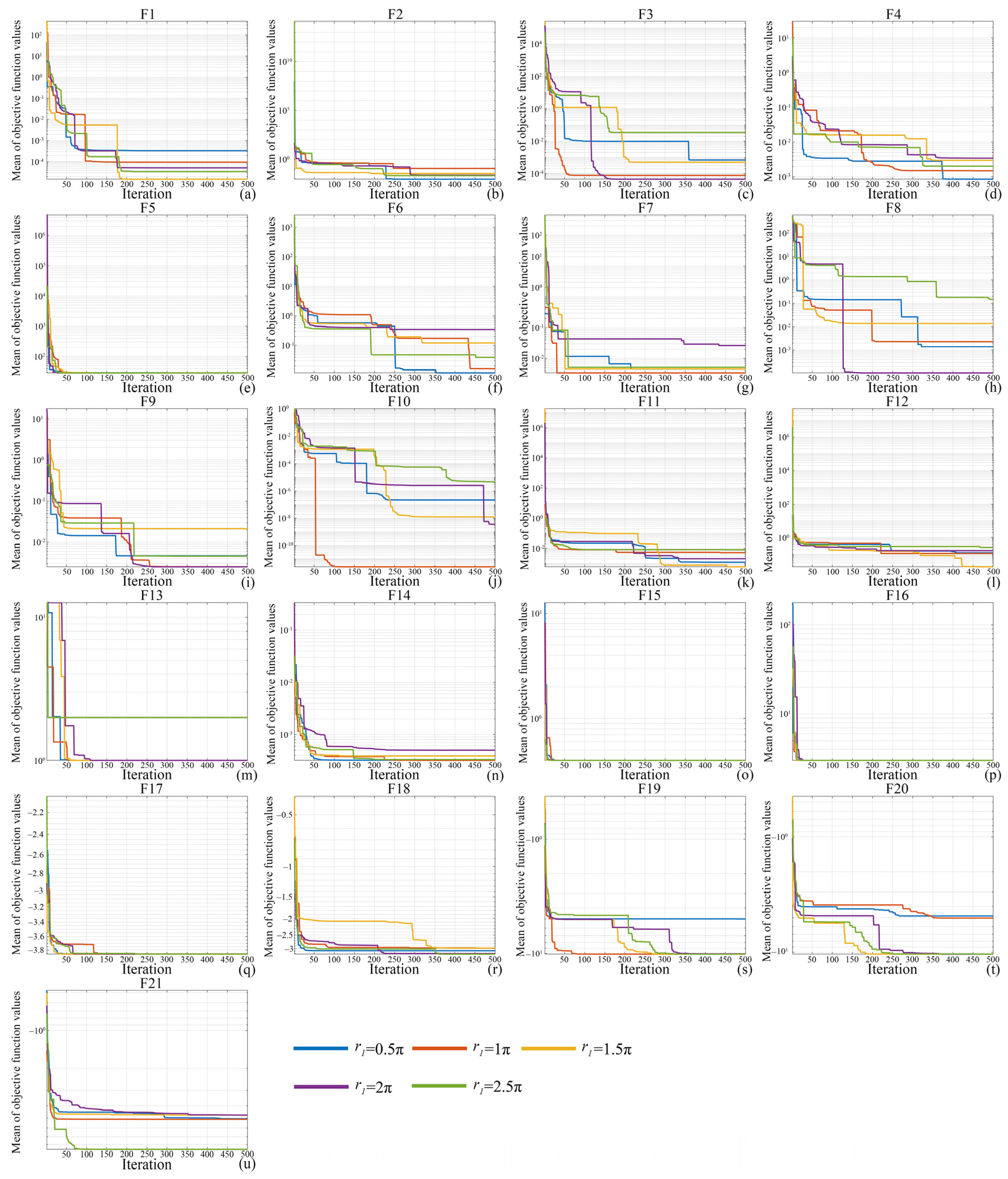
For the sine control parameter r1 in the golden sine strategy, five gradient levels are set for analysis: 0.5π, 1π, 1.5π, 2π, and 2.5π. Experimental results reveal that r1 = 0.5π ranks first across all gradient levels, corresponding to the optimal comprehensive performance (see Table A2).
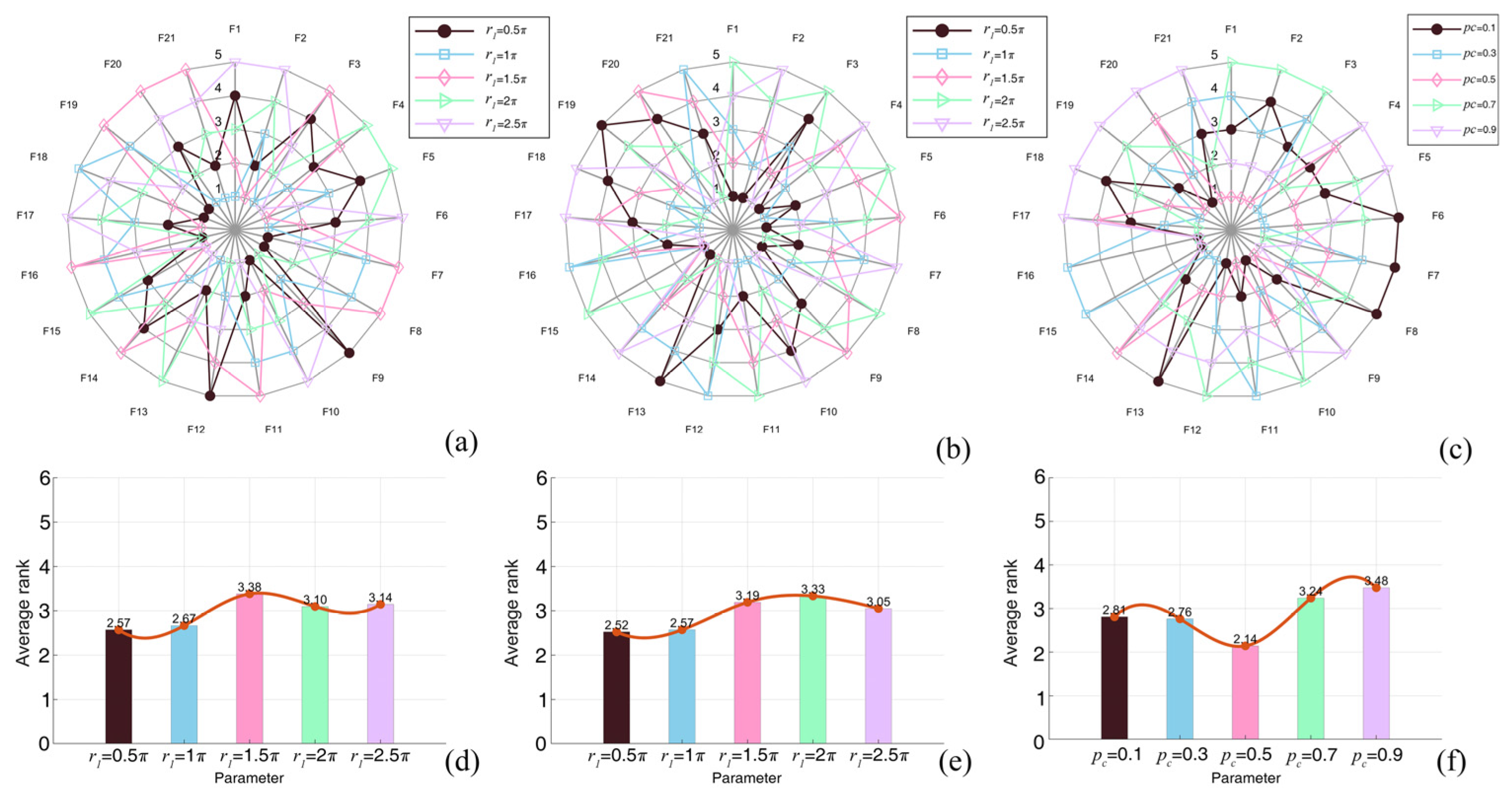
The convergence characteristics of the IHLOA with different r1 values on benchmark functions are shown in Figure 2. From the perspective of different function categories, r1 = 0.5π maintains exceptional optimization precision on unimodal functions F1–F4, achieves stable global search performance on multimodal functions F5–F10, and also exhibits outstanding solution capability for complex problems on composite functions F19–F21. Regarding result stability, the standard deviation of the majority of test functions remains at a low level under r1 = 0.5π; specifically, the std of F13 is as low as 1.00 × 10⁻⁸, and that of F15 is only 1.30 × 10⁻⁷, which strongly demonstrates the excellent robustness of the algorithm under this parameter setting. As r1 increases beyond 1π, the average ranking value of the algorithm rises significantly, accompanied by a continuous deterioration in comprehensive performance. Mechanistically, an excessively large r1 amplifies the stochasticity of the search process, undermines the local exploitation capability of the algorithm, and ultimately results in a synchronous degradation of both optimization accuracy and result stability.

3.1.2. Sensitivity Analysis of Sine Parameter r2

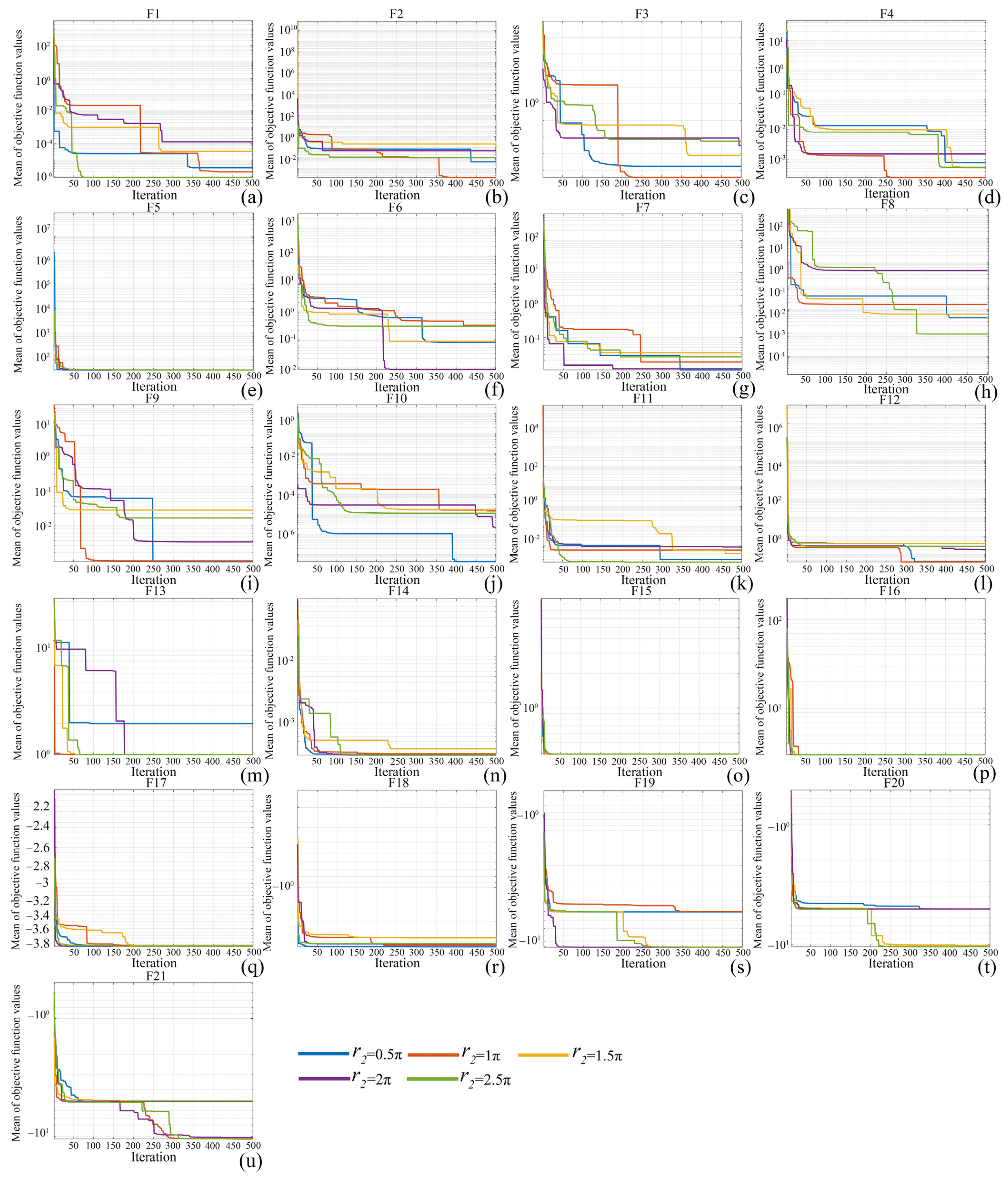
For the sine control parameter r2 in the golden sine strategy, five gradient levels are configured for analysis: 0.5π, 1π, 1.5π, 2π, and 2.5π. The results demonstrate that r2 = 0.5π ranks first across all tested gradients, delivering the best comprehensive algorithmic performance (see Table A3).
On unimodal test functions, r2 = 0.5π attains extremely high optimization accuracy, with the avg of F1 reaching as low as 1.47 × 10⁻⁵ and the avg of F2 being merely 1.74 × 10⁻², both of which are the optimal values obtained across all gradient levels for this parameter. Meanwhile, the std values of functions, including F15, are 0, further validating the superior stability of the optimization results under this setting. As the value of r2 increases, the average ranking value of the algorithm exhibits a consistent upward trend, indicating continuous performance degradation. An excessively large r2 will induce uncontrolled search step size and excessive fluctuations in population diversity, which ultimately leads to a marked decline in both optimization accuracy and result robustness. The convergence characteristics of the IHLOA with different r2 values on benchmark functions are shown in Figure 3.

3.1.3. Sensitivity Analysis of Crossover Probability pc

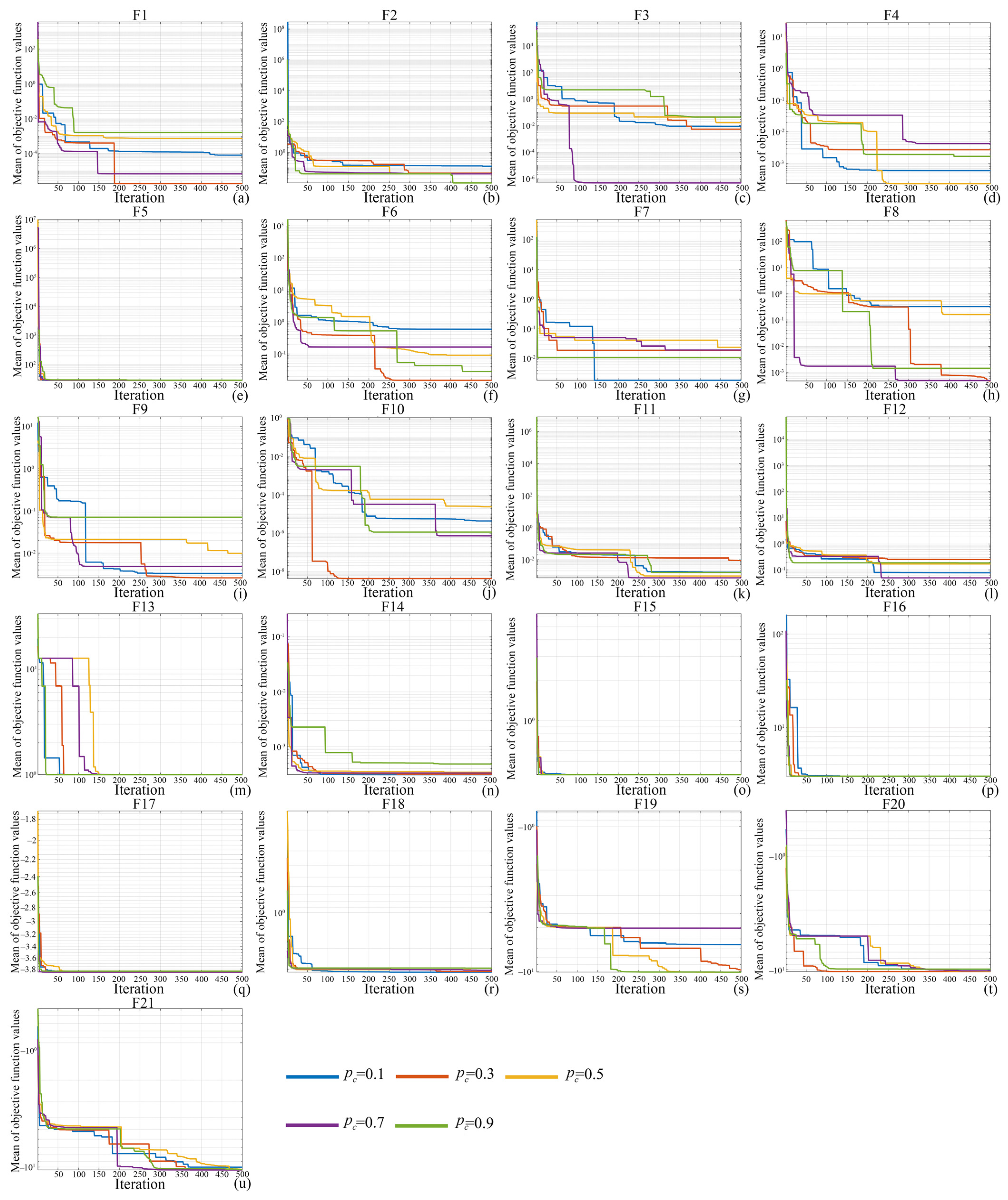
For the crossover probability pc in the orthogonal crossover strategy, five gradient levels are established for analysis: 0.1, 0.3, 0.5, 0.7, and 0.9. Experimental results confirm that pc = 0.5 ranks first across all gradient levels, with comprehensively superior performance on the entire test suite (see Table A4).
The crossover probability pc directly determines the intensity of information interaction between individuals in the population. The value of pc = 0.5 ensures efficient information exchange and knowledge transfer between individuals, while effectively preserving population diversity throughout the iterative process. Specifically, it circumvents the issue of insufficient inter-individual information exchange and slow convergence caused by an excessively small pc and also mitigates the drawback of disruption to high-quality individual schemas and degraded optimization accuracy induced by an excessively large pc. Across the entire test suite, the avg values of F1–F3 under pc = 0.5 are all optimal among all tested configurations for this parameter, and the overall optimization capability on composite functions F19 and F21 is also the most prominent. Furthermore, the std values of the majority of test functions are maintained at the lowest level under this setting, demonstrating that pc = 0.5 simultaneously achieves exceptional optimization accuracy and strong result robustness. The convergence characteristics of the IHLOA with different pc values on benchmark functions are shown in Figure 4.
Figure 5 presents the radar charts and average ranking results for the IHLOA parameter sensitivity analysis. The radar chart clearly illustrates the algorithm’s comprehensive performance under different parameter configurations: when set to the optimal values determined in this study, r1 = 0.5π, r2 = 0.5π, and pc = 0.5, the algorithm achieves optimal performance across all dimensions with the broadest coverage, validating its superior overall performance. As the parameters deviate from the optimal values, the algorithm’s performance declines with a marked reduction in coverage, consistent with the conclusions of the sensitivity analysis. Based on the comprehensive sensitivity analysis above, combined with the performance distribution visualized by the radar plots and the quantitative performance comparison from the average ranking plots, this paper determines the optimal parameter configuration for the improved HLOA as follows: the sine control parameters r1 = 0.5π and r2 = 0.5π for the golden sine strategy and the crossover probability pc = 0.5 for the orthogonal crossover strategy. With this optimized configuration, the algorithm consistently maintains superior comprehensive performance across unimodal, multimodal, and composite benchmark functions, rigorously validating the rationality of the selected parameters and the inherent stability and robustness of the proposed algorithm.

3.2. Ablation Experiment

To quantitatively verify the independent performance contribution and synergistic optimization effect of the three proposed improved strategies, namely, Fuch chaotic mapping, GSS and OCS, on the original HLOA, this section conducts ablation experiments based on classical benchmark test functions.

3.2.1. Experimental Design

To achieve single variable control, five algorithm groups are constructed for comparative analysis in this experiment: IHLOA is the optimized algorithm fully integrated with the three improved strategies; IHLOA_OCS is the ablation variant with only the orthogonal crisscross strategy removed from the IHLOA, which is used to verify the independent performance contribution of this strategy; IHLOA_Fuch is the ablation variant with only Fuch chaotic mapping removed from the IHLOA, which is used to verify the performance gain of this chaotic initialization strategy; IHLOA_GSS is the ablation variant with only the golden sine strategy removed from the IHLOA, which is used to verify the optimization effect of this position update mechanism; and HLOA is the original Horned Lizard Optimization Algorithm, serving as the baseline control group.
During the experiment, the basic hyperparameters such as population size and the maximum number of iterations of all algorithms are kept completely consistent, and each group of experiments is independently repeated 30 times to eliminate random errors. The Wilcoxon signed-rank test is employed to verify the statistical significance of performance differences between algorithms, with the significance level set to 5%.

3.2.2. Experimental Results and Analysis

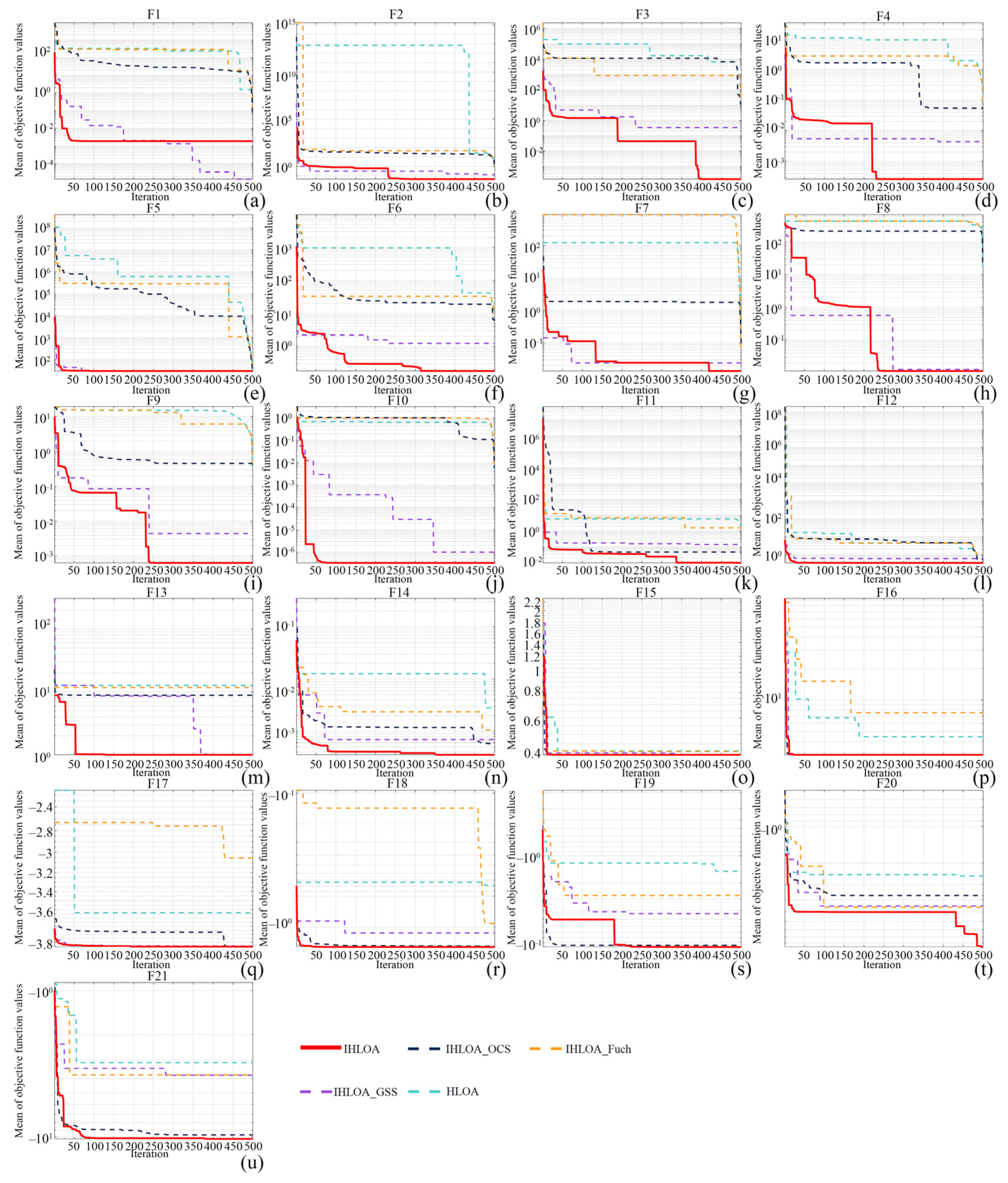
The results of the ablation experiment show that all three proposed improved strategies have significant positive gains on the performance of the HLOA, and the multi-strategy collaboration achieves the optimal balance between the global exploration and local exploitation capabilities of the algorithm. For the unimodal test functions F1–F7 for testing local exploitation capability, the complete IHLOA achieves the optimal convergence accuracy on most functions. Taking the high-dimensional unimodal function F3 as an example, the average optimal value of the IHLOA is 3.39 × 10⁻², which is at least two orders of magnitude higher than that of IHLOA_OCS, IHLOA_Fuch and the original HLOA, verifying the enhancement effect of the three strategies on the local exploitation capability of the algorithm. In functions such as F1 and F11, IHLOA_GSS shows the optimal single-point convergence accuracy, which proves the outstanding contribution of the golden sine strategy in the fine search of unimodal functions. The convergence characteristics of the full IHLOA and its various strategy ablation variants on classical benchmark test functions are intuitively reflected in Figure 6, which depicts the convergence curves of the IHLOA and its strategy ablation variants on benchmark functions.
The detailed performance data of each algorithm group in the ablation experiment is comprehensively recorded in Table A5. For the multimodal test functions F9–F13 for evaluating global exploration capability, the performance advantage of the IHLOA is more significant. Taking the multimodal function F9 as an example, the average optimal value of the IHLOA is 7.01 × 10⁻³, while the average optimal values of IHLOA_OCS, IHLOA_Fuch and the original HLOA all exceed 10, with the accuracy improved by more than two orders of magnitude. This result indicates that the three improved strategies can effectively enhance the global search ability of the algorithm and solve the premature convergence problem, wherein the original HLOA is prone to falling into local optima. For the composite test functions F14–F21 for simulating complex engineering optimization scenarios, the IHLOA shows overwhelming performance advantages. The average optimal values of F19, F20 and F21 reach −10.1, −9.99 and −10.4, respectively, all approaching the theoretical optimal values of the corresponding functions, while each ablation variant and the original HLOA have varying degrees of optimization failure, which fully verifies the effectiveness of the three strategies in dealing with complex optimization problems.
In terms of result stability, the standard deviation of the IHLOA is at the lowest level among all comparison groups in 21 test functions, among which the standard deviation of F15 is 0, which is much better than each ablation variant and the original HLOA, showing extremely strong robustness. The execution time of all comparison algorithms is in the same order of magnitude, and the proposed improved strategies do not bring additional computational burden to the algorithm, which ensures the engineering practicability of the algorithm.

3.2.3. Statistical Significance Test

The test results show that among all valid test functions, the p-values of the complete improved algorithm, the IHLOA, are less than the significance threshold of 0.05 on 21 test functions. This indicates that the performance improvement of the complete IHLOA over the original HLOA has extremely strong statistical significance, and the optimization effect is not caused by random experimental factors. For the algorithm variants integrated with only a single improved strategy, the number of functions with p-values less than the significance threshold of 0.05 for IHLOA_OCS and IHLOA_GSS compared with the original HLOA is 13 and 20, respectively. This result indicates that the improved strategies proposed in this paper can produce a statistically significant positive optimization effect on the performance of the original HLOA, which verifies the rationality and effectiveness of the design of each improved strategy from a statistical perspective. Meanwhile, the number of functions with a significant optimization effect achieved by the complete IHLOA is much higher than that of each single-strategy variant, which further proves that the synergistic effect of the three improved strategies can bring more stable and universal performance improvement to the algorithm. Even in the few functions where the performance difference does not reach a significant level, the average optimal value and standard deviation of the IHLOA are kept at the same level as the original HLOA without any performance degradation, which fully verifies the stability and scenario universality of the proposed algorithm.
For IHLOA_Fuch, integrated solely with Fuch chaotic mapping, the performance difference from the original HLOA fails to reach the 5% statistical significance level on most test functions, which stems from the inherent characteristics of the strategy’s action mechanism. The core function of Fuch chaotic mapping is to optimize the spatial distribution of individuals during population initialization and improve the ergodicity and diversity of the initial population, so as to provide a high-quality initial basis for algorithm iteration. It acts as a prepositive auxiliary optimization strategy, rather than a core strategy that directly modifies the iterative search mechanism. When integrated alone, it can only optimize the initial population quality but cannot fundamentally solve the core defects of the original HLOA, including the rapid decay of population diversity and vulnerability to local optima during iteration. Hence, its performance improvement is limited when acting independently, failing to reach the statistically significant level.

3.3. Performance Test of the Proposed IHLOA

To comprehensively verify the optimization performance of the proposed IHLOA, this section conducts comparative experiments under three different dimensional scales (30-D, 50-D, and 80-D) based on classical benchmark test functions. Eight classical meta-heuristic algorithms, including the original HLOA, PSO (Particle Swarm Optimization), the GOOSE algorithm, Ant Colony Optimization (ACO), the Social Ski-Driver (SSD) algorithm, the Escape algorithm (ESC), the Enhanced Gaining-Sharing Knowledge-based algorithm (eGSK), and the Heap-based (HBO) algorithm, are selected as the comparison groups. The comprehensive solution capability of the IHLOA is systematically quantified from five dimensions: convergence accuracy, robustness, high-dimensional scalability, statistical significance, and convergence characteristics.

3.3.1. Experimental Setup

In the experiment, core hyperparameters of all algorithms (population size = 30, maximum number of iterations = 500, etc.) were kept fully consistent. To eliminate the interference of random factors on the results, each group of experiments was independently repeated 30 times. The specific settings of algorithm parameters are shown in Table 1:

3.3.2. Analysis of Optimization Performance Results Under Different Dimensions

The experimental results show that the proposed IHLOA achieves the optimal convergence accuracy and the smallest standard deviation in most test functions under the three dimensions of 30-D, 50-D and 80-D. Its comprehensive performance is significantly better than all comparison algorithms, and it exhibits excellent scalability for high-dimensional problems.
The detailed optimization performance data of all algorithms in the 30-dimensional low-dimensional test scenario are fully recorded in Table A7. In the 30-D low-dimensional scenario, the performance advantage of the IHLOA has been fully reflected. For unimodal test functions, the IHLOA achieves convergence accuracy far superior to the comparison algorithms in F1–F5. Among them, the average optimal value of F1 is as low as 1.09 × 10⁻⁴, which is three orders of magnitude higher than the 8.27 × 10⁻² of the original HLOA, while the average optimal values of classical algorithms such as PSO and ACO all exceed the order of 1 × 101, fully verifying the extremely strong local exploitation capability of the IHLOA. For multimodal test functions, the IHLOA shows overwhelming performance advantages in F8–F11. The average optimal value of F8 is only 1.53 × 10⁻², while the results of the original HLOA and other comparison algorithms all exceed the order of 10, proving that the IHLOA can effectively escape from local optima and has an extremely strong global exploration capability. For composite test functions, the average optimal values of the IHLOA in F19–F21 reach −10.2, −10.4 and −8.82, respectively, all approaching the theoretical optimal values of the corresponding functions, while all comparison algorithms have varying degrees of optimization failure, verifying the excellent solution capability of the IHLOA in complex optimization problems.
As the problem dimension increases to 50-D and 80-D, the performance of all comparison algorithms deteriorates significantly, while the IHLOA still maintains stable, high-precision solution capabilities, showing extremely strong high-dimensional scalability. The specific optimization performance data of all algorithms in the 50-D and 80-D high-dimensional scenarios are presented in Table A8 and Table A9, respectively. Taking the high-dimensional unimodal function F1 as an example, when the dimension increases from 30-D to 80-D, the average optimal value of the original HLOA deteriorates from 8.27 × 10⁻² to 1.58, and the result of the PSO algorithm deteriorates from 27.9 to 6.05 × 10³, while the average optimal value of the IHLOA only changes from 1.09 × 10⁻⁴ to 8.16 × 10⁻³, always maintaining extremely high convergence accuracy. In the 80-D multimodal function F8 and composite function F19, the average optimal values of the IHLOA are 1.67 and −10.1 respectively, which are still far better than all comparison algorithms, and the standard deviation is always at the lowest level. The results show that the “curse of dimensionality” caused by the increase in dimension has a much smaller impact on the IHLOA than other comparison algorithms, and the proposed improved strategies effectively solve the problem of sudden performance degradation of meta-heuristic algorithms in high-dimensional problems.

3.3.3. Statistical Significance Analysis

To verify that the performance advantage of the IHLOA is not caused by experimental random errors, the Wilcoxon signed-rank test is carried out with a significance level of 5% based on the experimental results of 30 independent runs. The test results quantify the statistical significance of the performance difference between the IHLOA and each comparison algorithm. The specific statistical test results of all algorithms in the 30-D, 50-D and 80-D scenarios are detailed in Table A10, Table A11 and Table A12, respectively.
In the 30-D scenario, the p-values of the IHLOA compared with the original HLOA are less than the significance threshold of 0.05 in 20 out of 21 valid test functions. Compared with the other seven comparison algorithms (PSO, GOOSE, ACO, SSD, ESC, eGSK, HBO), the number of functions with p-values less than 0.05 is more than 10. In the 50-D and 80-D high-dimensional scenarios, the statistical advantage of the IHLOA is further expanded. In the 80-D scenario, the p-values of the IHLOA compared with all eight comparison algorithms are less than 0.05 in most test functions, and a significant difference is not reached only in a very small number of functions. This result fully proves that the performance improvement of the IHLOA compared with the comparison algorithms has strict statistical significance and is not caused by random factors. Even in a few functions with p-values greater than 0.05, the average optimal value and standard deviation of the IHLOA are kept at the same level as the optimal comparison algorithm in the corresponding scenario without any performance degradation, which further verifies the universality and stability of the algorithm.

3.3.4. Convergence Characteristic Analysis

Based on the average convergence curves of 30 independent runs in the 30-D scenario, the convergence speed and iterative optimization characteristics of the IHLOA are further analyzed. The convergence curve reflects the change trend of the average objective function value during the iteration process of the algorithm. The faster the curve descends and the lower the final convergence value, the faster the convergence speed and the stronger the optimization capability of the algorithm.
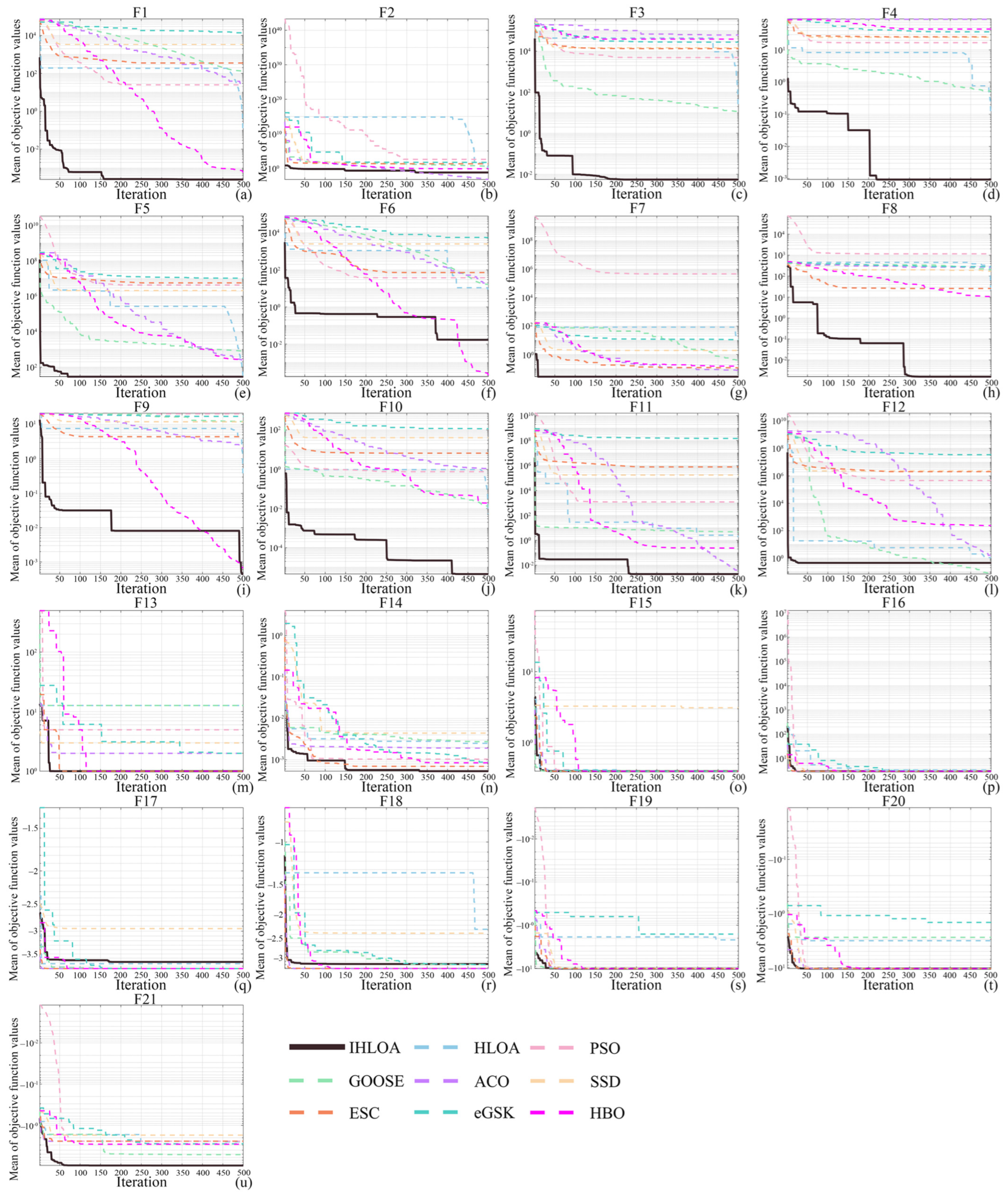
It can be seen from the convergence curves in Figure 7 that the IHLOA shows the fastest convergence speed and the best convergence effect in all test functions. In the unimodal test functions F3–F5, the convergence curve of the IHLOA presents an extremely fast downward trend at the initial stage of iteration, converges to an extremely low objective function value much earlier than all comparison algorithms, and does not appear to stagnate during the whole iteration process, which fully verifies its extremely strong local exploitation capability and fast convergence characteristics. In the multimodal test functions F9–F13, the convergence curves of most comparison algorithms tend to be flat in the middle stage of iteration, falling into local optima and being unable to continue optimization, while the curve of the IHLOA always maintains a steady decline, can continuously escape from local optimal traps, and keeps approaching the high-quality optimal solution, showing excellent global exploration capability. In the composite test functions F14–F21, the IHLOA still maintains a stable convergence trend, can continuously complete the solution optimization during the whole iteration process, and finally converges to a result close to the theoretical optimal value, while other comparison algorithms have varying degrees of optimization stagnation and cannot effectively solve complex composite optimization problems. In addition, the convergence curve of the IHLOA has very little fluctuation in multiple independent runs, which is consistent with the analysis results of the standard deviation and further verifies the robustness and result repeatability of the algorithm.
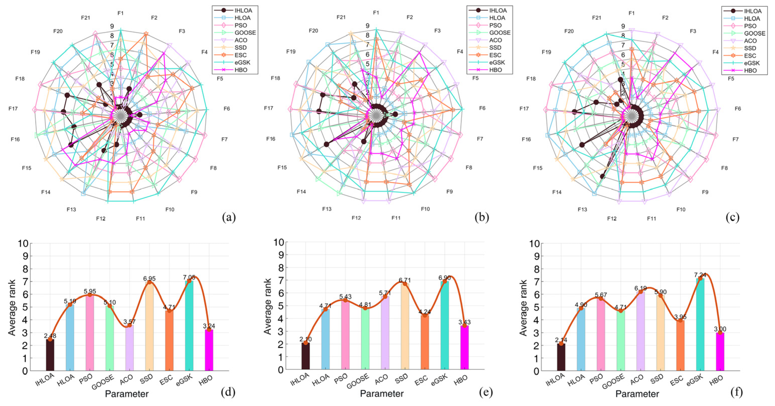
Figure 8 visually illustrates the comprehensive performance comparison and quantitative ranking of the IHLOA and all of the comparative algorithms across various dimensional scales. Specifically, the radar charts characterize the overall performance of each algorithm through the enclosed area across dimensions, where a smaller area indicates superior performance. It can be observed that the IHLOA achieves the smallest enclosed area across all test function dimensions, reflecting its optimal overall optimization capability. In contrast, the remaining comparison algorithms exhibit larger coverage areas, indicating performance gaps of varying degrees. The average ranking plots quantify performance using numerical values, with lower values corresponding to better overall performance. The IHLOA consistently attains the lowest average ranking across all dimensions, further validating its stability and superiority in multi-dimensional test scenarios. Overall, the IHLOA maintains an advantageous position across all indicators, with comprehensive performance that is clearly superior to that of the other algorithms.
Based on the comprehensive results of performance tests across different dimensions, statistical significance tests, and convergence characteristic analyses, the proposed IHLOA demonstrates significant superiority over the original HLOA and seven other classical meta-heuristic algorithms in four core dimensions: convergence accuracy, robustness, convergence speed, and high-dimensional scalability. This fully validates the synergistic optimization effect of the three proposed improvement strategies (Fuch chaotic mapping, the golden sine strategy, and the orthogonal crisscross strategy), as well as the excellent solution capability of the IHLOA in complex optimization problems.
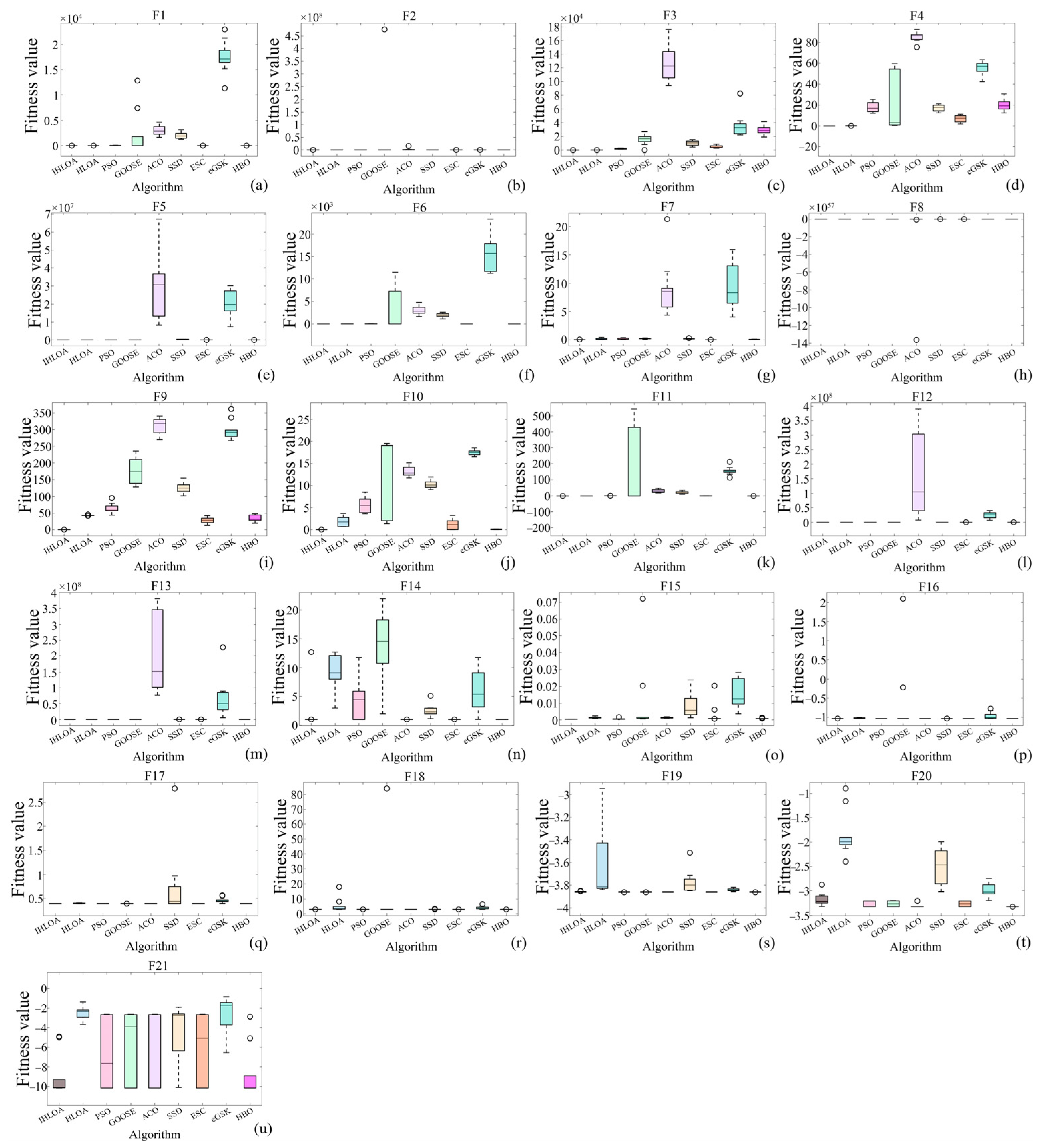
As observed from the box plots in Figure 9, on most test functions, the box of the IHLOA is positioned significantly lower than those of the comparative algorithms, indicating higher convergence accuracy. Meanwhile, the interquartile range of the IHLOA box is narrower and there are fewer outliers, demonstrating stronger convergence stability and effective avoidance of local optima. Compared with the original HLOA, the IHLOA significantly improves the balance between global exploration and local exploitation by introducing Fuch chaotic mapping, the golden sine strategy, and the orthogonal crossover strategy, fully validating the effectiveness and superiority of the proposed improvement strategies.

3.4. Path Planning Experiment

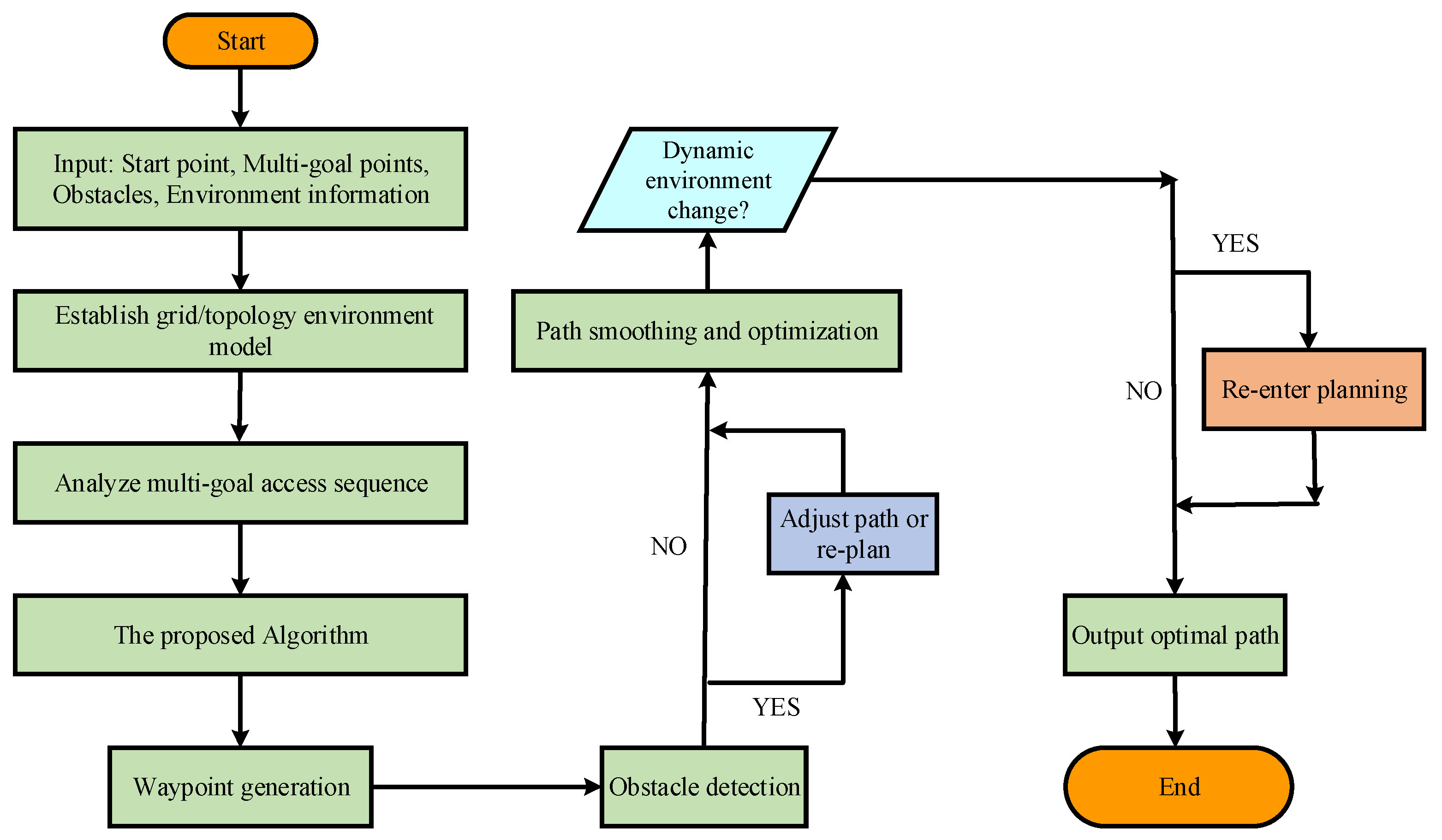
To further verify the effectiveness and optimization performance of the proposed IHLOA in path planning, the grid method is used to model the known environment, and all experiments are carried out on the MATLAB R2023a simulation platform (MathWorks, Natick, MA, USA). The side length of each grid is 1 m. In the simulation map, black grids represent obstacles, white grids denote feasible regions, and the start and end points are set at the lower-left and upper-right corners of the map, respectively. To test the algorithm’s performance under different environmental complexity levels, grid environments with varying obstacle ratios are artificially designed and constructed. The obstacle ratio is defined as the proportion of obstacle grids to the total number of grids in the entire map. The parameters of the IHLOA and the HLOA, such as population size and maximum number of iterations, are consistent with those in the benchmark function experiments. The detailed path planning simulation parameters are listed in Table 2. The overall workflow of the path planning experiment is illustrated in Figure 10.

3.4.1. Single-Goal Path Planning

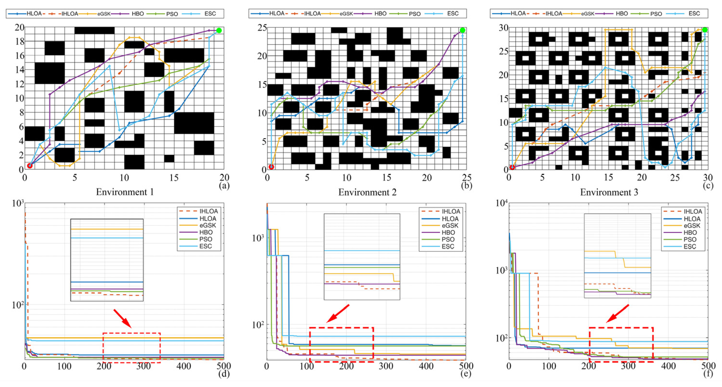
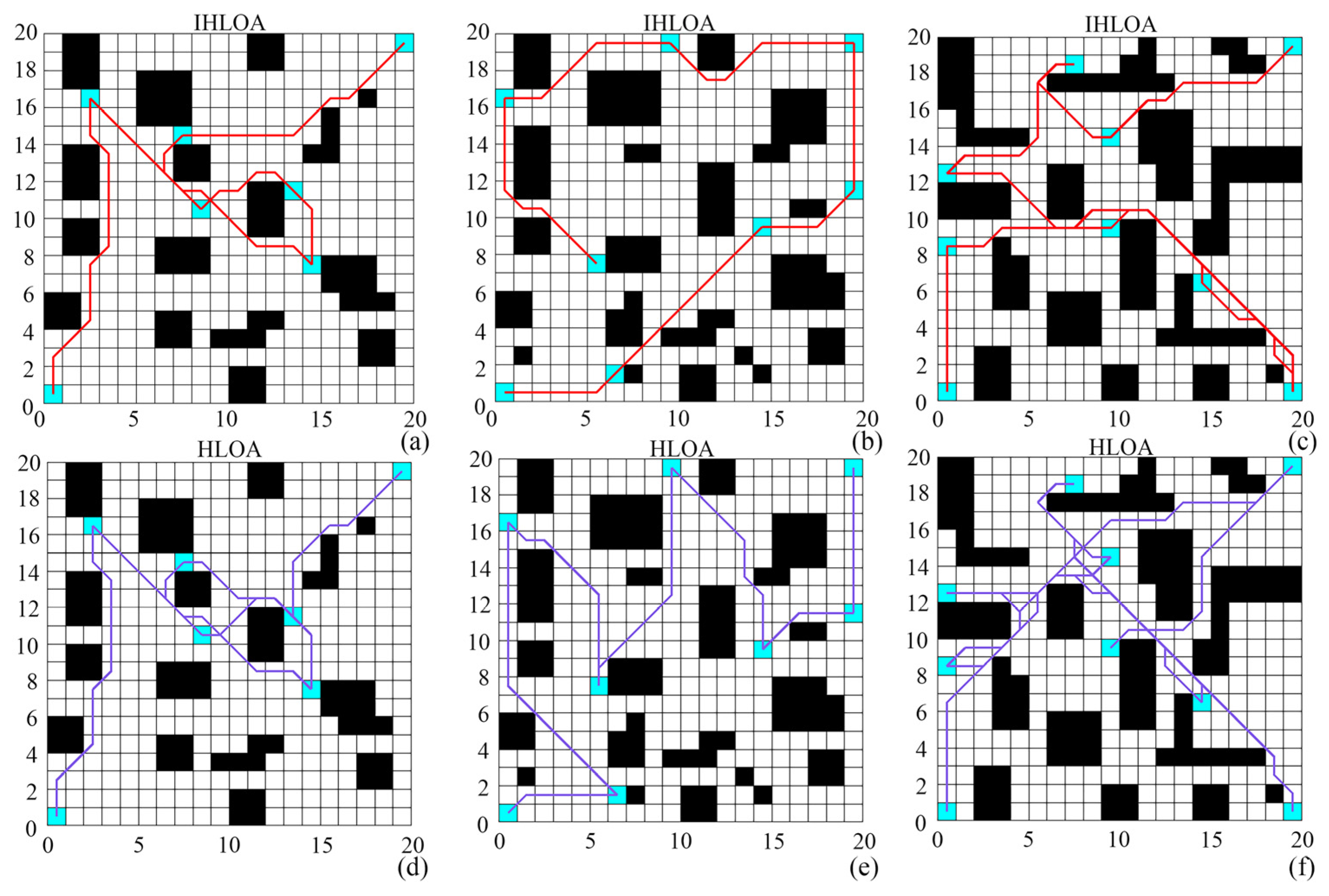
To comprehensively evaluate the performance of the proposed IHLOA in path planning tasks, multi-scale comparative simulation experiments were conducted on 20 × 20, 25 × 25 and 30 × 30 single-objective grid maps, with the HLOA, eGSK, HBO, PSO and ESC selected as the comparison algorithms. To ensure the fairness and reliability of the experiments, all algorithms were configured with the same core hyperparameters, and each test was independently repeated 100 times to eliminate the interference of random factors. The core quantitative performance indicators of all algorithms, including the minimum path length and the number of turning points, are statistically summarized in Table 3, and the path planning trajectory visualization results are shown in Figure 11.
The experimental results demonstrate that the IHLOA achieves the optimal performance in all grid-scale environments, consistently obtaining the shortest minimum path length and the fewest turning points among all compared algorithms. In terms of the minimum path length, the IHLOA outperforms the comparison algorithms by 2.54–87.64%, and the performance advantage is more prominent with the increase in grid scale and environmental complexity; in terms of the number of turning points, the IHLOA reduces this by 9.09–109.09% compared with other algorithms, which reflects its superior ability to generate smooth paths. Notably, the IHLOA maintains stable and excellent optimization performance even in the 30 × 30 large-scale complex grid environment without obvious performance degradation, while the comparison algorithms are prone to path redundancy and significant performance decline in complex environments due to defects such as weak global exploration ability. Combined with the trajectory visualization in Figure 1, the path generated by the IHLOA is collision-free with no redundant detours, and the overall smoothness is significantly better than that of the comparison algorithms. These results fully verify the effectiveness of the improved strategies of the IHLOA in enhancing path planning performance and also prove the strong robustness and adaptability of the algorithm in grid map environments of different scales.

3.4.2. Simulation and Analysis of Static Multi-Goal Path Planning

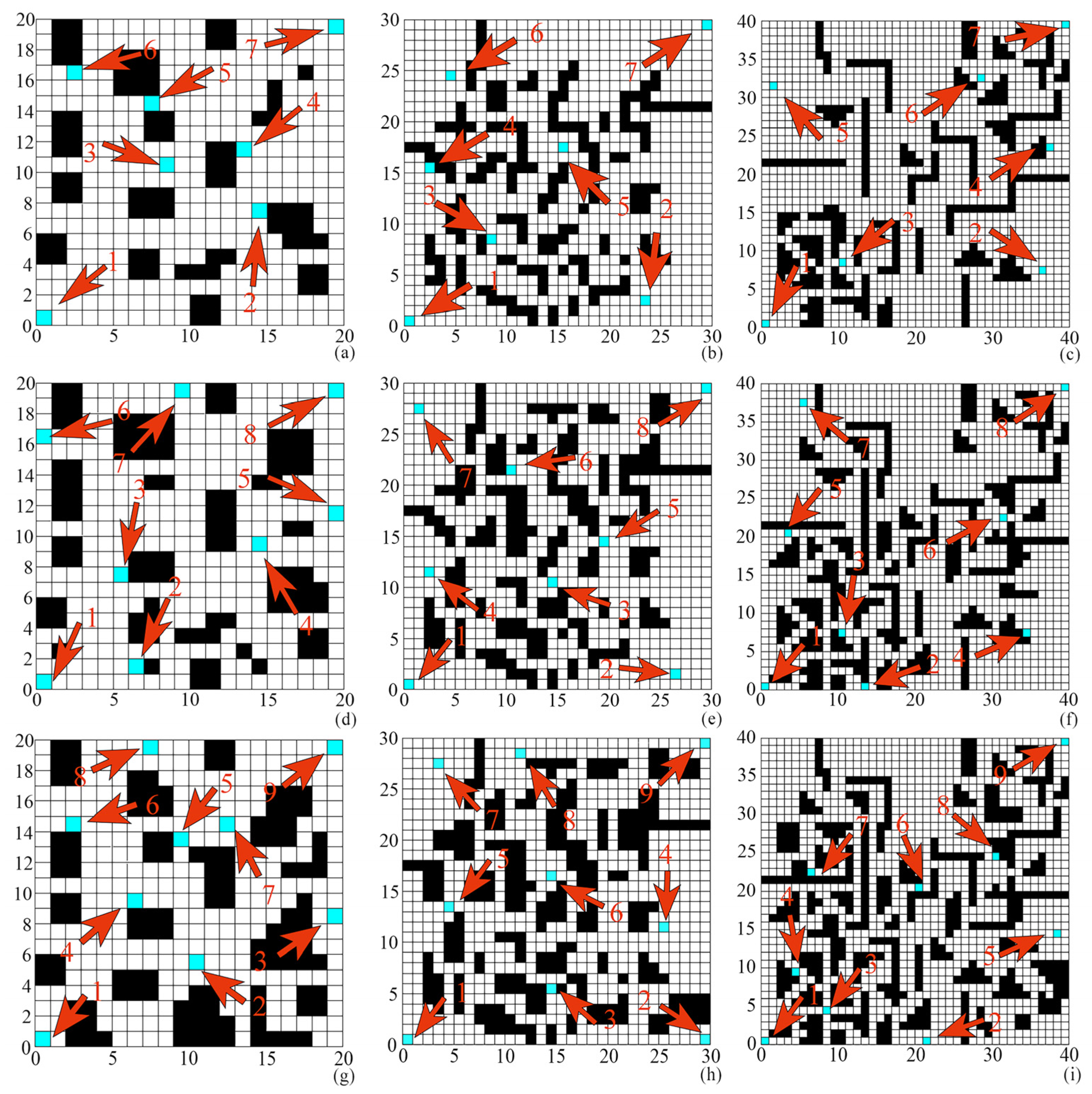
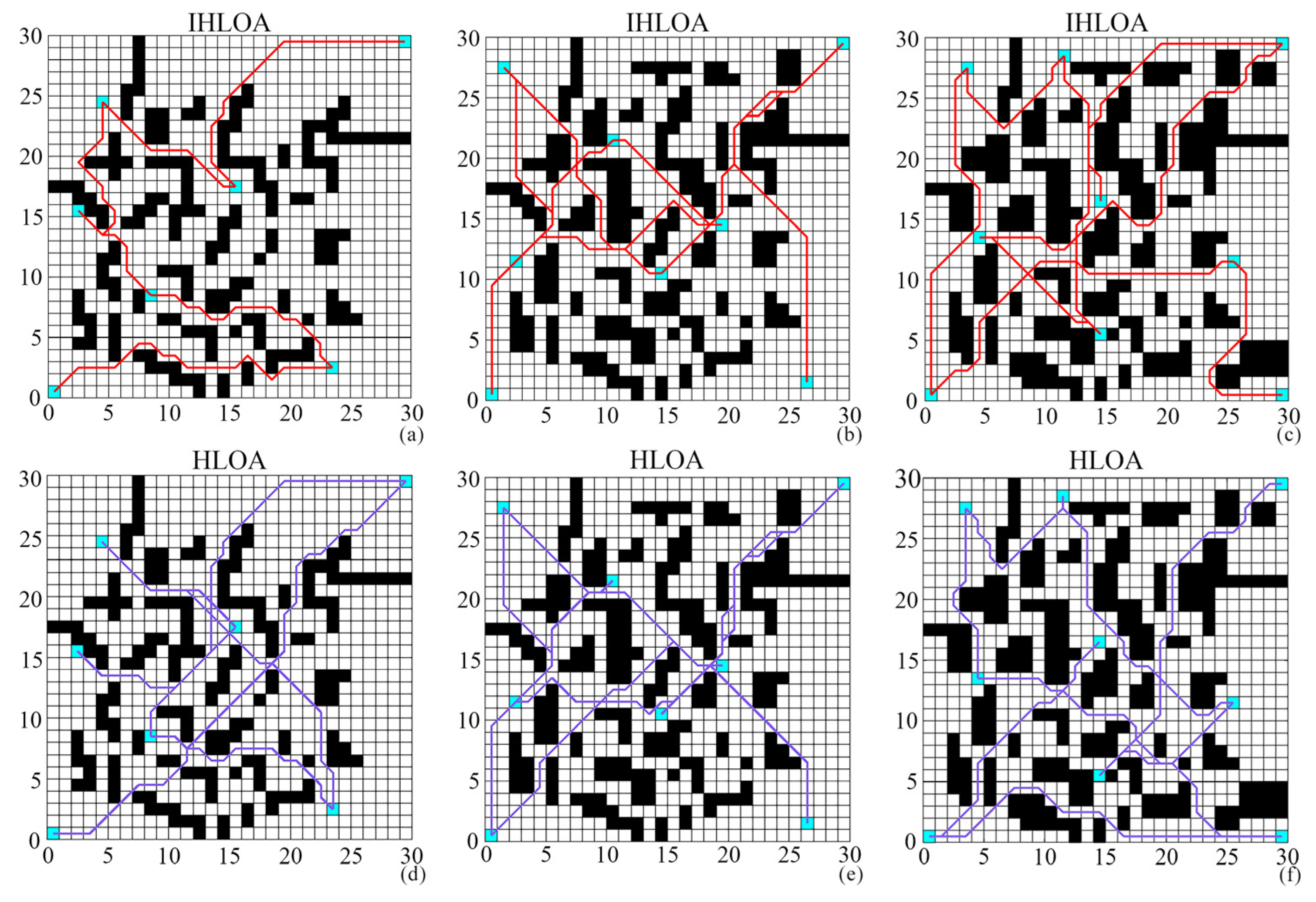
Comparative simulation experiments of the IHLOA and the HLOA are conducted on multi-goal grid maps of varying sizes (including 20 × 20, 30 × 30, and 40 × 40 grids), where grid maps with different complexities are constructed using diverse obstacle rates. Both algorithms adopt the same initial population size and a unified maximum iteration number of 500. Each algorithm is independently run 50 times, with average values taken as the final results. The uniform parameter settings ensure experimental fairness, while multiple independent runs mitigate the impact of random factors, enhancing the reliability and stability of the results. The distributions of multiple goal points are illustrated in Figure 12. The corresponding path planning results on 20 × 20, 30 × 30, and 40 × 40 grids are displayed in Figure 13, Figure 14 and Figure 15, respectively. The path trajectories and metric test results are presented below.
Table 4 reveals that in 20 × 20 path planning with an obstacle rate of 0.2, the IHLOA reduces the minimum path length by 5.55% compared to the HLOA. In the 40 × 40 scenario with an obstacle rate of 0.3, the minimum path length is reduced by 7.99%, demonstrating the IHLOA’s higher convergence accuracy and path planning efficiency in multi-goal path planning. On the 30 × 30 grid and with an obstacle rate of 0.3, the IHLOA achieves a 3.67% reduction in minimum path length compared to the HLOA. Table 5 indicates that on a 40 × 40 map with an obstacle rate of 0.2, the IHLOA has 18 fewer turning points than the HLOA; when the obstacle rate increases to 0.25, the number of turning points is still reduced by 17, validating the IHLOA’s effectiveness in avoiding local optima and generating paths with significantly better comprehensive quality than the HLOA. Experimental data demonstrate that the IHLOA consistently plans shorter paths across multi-scale maps and varying obstacle rates, significantly outperforming the HLOA in searching for multiple goal points in complex environments. Its optimization efficiency improves with increasing environmental complexity, showcasing stronger robustness and environmental adaptability.

3.4.3. Simulation and Analysis of Dynamic Multi-Goal Path Planning

To verify the effectiveness of the IHLOA in dynamic environment path planning, we compare it with the HLOA on two types of grid maps and integrate the dynamic window approach (DWA) to realize local dynamic obstacle avoidance. The IHLOA optimizes the initial population distribution via Fuch chaotic mapping, balances global exploration and local exploitation using the golden sine strategy, and enhances population information interaction through the orthogonal crossover strategy, addressing the limitations of the original HLOA, such as susceptibility to local optima, slow convergence, and insufficient obstacle avoidance robustness in dynamic scenarios. As shown in the quantitative indicators of Table 6, in obstacle-dense Map 1, the IHLOA reduces the total path length by 77.3%, cuts the total simulation steps and running time by 54.9%, shortens the actual trajectory length by 36.0%, and decreases the robot stuck times by 61.5%. In obstacle-sparse Map 2, performance improvements of 18.2–24.7% are still achieved across all indicators, and neither algorithm experiences replanning failures. Combined with the path visualization results in Figure 16, the red HLOA trajectory is prone to local oscillations and detours when avoiding dynamic obstacles, while the blue IHLOA trajectory can quickly escape local optima to generate smoother and shorter feasible paths, fully validating the significant advantages of the improved strategies in enhancing the efficiency, robustness, and trajectory quality of dynamic path planning.
Although the IHLOA achieves outstanding performance in grid-based simulations, transferring the algorithm to real-world robotic systems involves non-negligible practical challenges. In physical environments, sensor measurements are inevitably corrupted by noise, and localization systems suffer from drift or mismatching errors, which may degrade the input accuracy of path planning. Meanwhile, dynamic obstacles in real scenarios show more random and unpredictable motion patterns compared with simulation settings. In addition, the kinematic constraints, actuator delays, and limited computing power of physical robots further increase the difficulty of practical deployment. In the future, we will focus on robust strategies against noise and errors, dynamic prediction mechanisms, and computational efficiency optimization to bridge the simulation-to-reality gap and promote the practical application of the proposed algorithm.

4. Conclusions

To address the inherent defects of the original Horned Lizard Optimization Algorithm (HLOA), such as uneven initial population distribution, weak balance between global exploration and local exploitation, insufficient inter-individual information interaction, and proneness to premature convergence, this paper proposes an Improved Horned Lizard Optimization Algorithm (IHLOA) by integrating Fuch chaotic mapping, the golden sine strategy, and the orthogonal crossover strategy. Comprehensive experimental evaluations based on benchmark test functions and practical path planning scenarios fully verify that the proposed algorithm effectively fills the research gaps in existing optimization algorithms, achieving significant performance advantages compared to traditional methods and state-of-the-art meta-heuristic algorithms, thus providing valuable references for the field of bio-inspired meta-heuristic optimization.
In the benchmark function tests across 30-D, 50-D, and 80-D scenarios, the IHLOA outperforms comparative algorithms (including the HLOA, PSO, ACO, eGSK, etc.) in optimization accuracy, convergence speed, robustness, and high-dimensional scalability. Specifically, the IHLOA rapidly converges to near-theoretical optimal values in unimodal functions with standard deviations approaching zero, exhibits strong capability in escaping local optima in multimodal functions, and maintains stable optimization performance in complex composite functions. Statistical significance tests confirm that the performance improvement of the IHLOA is statistically significant in most test functions, excluding random experimental errors. Ablation experiments further demonstrate the synergistic optimization effect of the three improved strategies: Fuch chaotic mapping optimizes initial population distribution, the golden sine strategy balances exploration and exploitation, and the orthogonal crossover strategy enhances information interaction, all of which are indispensable for the performance leap of the IHLOA.
In practical path planning applications, the IHLOA shows remarkable performance in single-goal, multi-goal, and dynamic obstacle environments. In single-goal path planning across 20 × 20, 25 × 25, and 30 × 30 grid maps, the IHLOA reduces path length by 2.54–87.64% and turning points by 9.09–109.09% compared to comparative algorithms. In multi-goal path planning, it achieves a 1.24–7.99% reduction in path length and an 11.91% average reduction in turning points relative to the original HLOA. In dynamic obstacle environments, the IHLOA shortens the path length by 18.2–77.3% and reduces robot stuck times by 20.0–61.5%, while maintaining no replanning failures. Although the time complexity of the IHLOA is O(2 × T × N × (D + FE))—slightly higher than the original HLOA’s O(T × N × (D + FE))—the computational overhead increase is negligible (within the same order of magnitude), and the trade-off is well-justified by the significant improvements in path quality (shorter length, fewer turning points) and robot operational efficiency (lower energy consumption and motion control cost).
Despite the superior performance, the IHLOA still has certain limitations that need to be addressed in future research. Firstly, the algorithm’s parameter configuration is determined based on sensitivity analysis under specific experimental settings, and its adaptability to dynamically changing complex environments (e.g., time-varying obstacle densities, unknown terrain) remains to be verified. Secondly, the IHLOA is currently designed for grid-based path planning, and its applicability to continuous space, 3D complex terrain, and multi-robot collaborative path planning scenarios requires further expansion. Thirdly, the algorithm’s optimization mechanism does not fully consider real-time constraints in practical applications (e.g., robot motion dynamics, sensor measurement noise), which may affect its engineering implementation effect. Fourth, all experiments in this study are implemented in grid-based simulation environments. Although the proposed IHLOA exhibits excellent performance in static and dynamic path planning scenarios, practical deployment on physical robotic platforms still faces several realistic challenges, including sensor noise, odometry drift, localization errors, uncertain dynamic obstacles, kinematic constraints, actuator delays, and limited on-board computing resources. These simulation-to-reality gaps need to be further addressed to enhance the engineering applicability of the algorithm.
The preferred application scope of the IHLOA includes static/dynamic grid environments with known obstacle distribution, such as indoor robot navigation, warehouse logistics scheduling, and unmanned ground vehicle path planning in structured scenes. It is particularly suitable for scenarios requiring high path smoothness and optimization accuracy, where the slight increase in computational complexity can be compensated by the reduced energy consumption and operational cost of the robots.
Future research directions will focus on the following aspects: (1) developing an adaptive parameter adjustment mechanism to enhance the algorithm’s adaptability to complex dynamic environments without manual tuning; (2) extending the algorithm’s framework to 3D space and continuous terrain and integrating robot motion constraints (e.g., maximum speed, turning radius) to improve engineering practicality; (3) exploring the fusion of the IHLOA with deep learning methods (e.g., neural network-based environment modeling) to address path planning problems in unknown environments; and (4) investigating the application of the IHLOA in multi-robot collaborative path planning and designing efficient task allocation and conflict avoidance mechanisms to improve overall operational efficiency. In addition to robot path planning, the proposed IHLOA also possesses strong generalization ability for other complex optimization scenarios. The three improvement strategies, including Fuch chaotic mapping, the golden sine strategy, and the orthogonal crossover strategy, are universal meta-heuristic enhancement mechanisms rather than domain-specific designs. Therefore, the IHLOA can be further extended to various high-dimensional and non-convex optimization problems, such as feature selection, neural network weight training, task scheduling, engineering parameter optimization, and multi-objective decision-making.


Author Contributions

B.Y.: investigation, software, data curation, formal analysis and writing—original draft. H.L.: conceptualization, methodology, supervision and writing—review and editing. L.D.: validation, visualization, formal analysis and software. H.D.: conceptualization, validation and funding acquisition. All authors have read and agreed to the published version of the manuscript.
Funding

This work was supported by Lianyungang City Science and Technology Plan Funding Project of Jiangsu Province (JCYJ2434, JCYJ2510, CG2521); Lianyungang High-level Talent Training Project (LYG065212025037).

Institutional Review Board Statement

Not applicable.

Informed Consent Statement

Not applicable.

Data Availability Statement

The original contributions presented in this study are included in the article. Further inquiries can be directed to the corresponding author.

Acknowledgments

The authors gratefully acknowledge the financial support from the Lianyungang Science and Technology Bureau and the technical assistance provided by the School of Mechatronic Engineering, China University of Mining and Technology.

Conflicts of Interest

The authors declare no conflicts of interest.

Appendix A

Table A1. Benchmark test functions.
Test FunctionnSfmin
f 1 x = i = 1 n x i 2 30[−100, 100]n0
f 2 x = i = 1 n x i + i = 1 n x i 30[−10, 10]n0
f 3 x = i = 1 n j 1 i x j 2 30[−100, 100]n0
f 4 x = max i x i , 1 i n 30[−100, 100]n0
f 5 x = i = 1 n 1 100 x i + 1 x i 2 2 + x i 1 2 30[−30, 30]n0
f 6 x = i = 1 n x i + 0.5 2 30[−100, 100]n0
f 7 x = i = 1 n i x i 4 + r a n d o m 0 , 1 30[−1.28, 1.28]n0
f 8 ( x ) = i = 1 n x i 2 10 cos ( 2 π x i ) + 10 30[−5.12, 5.12]n0
f 9 x = 20 exp 0.2 1 n i = 1 n x i 2 exp 1 n i = 1 n cos ( 2 π x i ) + 20 + e 30[−32, 32]n0
f 10 ( x ) = 1 4000 i = 1 n x i 2 i = 1 n cos x i i + 1 30[−600, 600]n0
f 11 ( x ) = π n 10 sin 2 π y i + i = 1 n 1 y i 1 2 1 + 10 sin 2 π y i + 1 + y n 1 2 + i = 1 n u x i , 10 , 100 , 4 ,
y i = 1 + x i + 1 4
u x i , a , k , m = k x i a m , x i > a , 0 , a < x i < a , k x i a m , x i < a .
30[−50, 50]n0
f 12 ( x ) = 0.1 sin 2 3 π x i + i = 1 n x i 1 2 1 + sin 2 3 π x i + 1 + x n 1 2 1 + sin 2 2 π x n + i = 1 n u x i , 5 , 100 , 4 30[−50, 50]n0
f 13 ( x ) = 1 500 + j = 1 25 1 j + i = 1 2 x i a i j 6 1 2[−65.536, 65.536]n1
f 14 ( x ) = i = 1 11 a i x i b i 2 + b 1 x 2 b i 2 + b 1 x 3 + x 4 2 4[−5, 5]n3.075 × 10−4
f 15 ( x ) = x 2 5.1 4 π 2 x 1 2 + 5 π x 1 6 2 + 10 1 1 8 π cos x 1 + 10 2[−5, 10] × [0, 15]0.398
f 16 ( x ) = 1 + x 1 + x 2 + 1 2 ( 19 14 x 1 + 3 x 1 2 14 x 2 + 6 x 1 x 2 + 3 x 2 2 ) × 30 + ( 2 x 1 3 x 2 ) 2 ( 18 32 x 1 + 12 x 1 2 + 48 x 2 36 x 1 x 2 + 27 x 2 2 ) 2[−2, 2]n3
f 17 ( x ) = i = 1 4 c i exp j = 1 3 a i j x j p i j 2 4[0, 1]n−3.86
f 18 ( x ) = i = 1 4 c i exp j = 1 6 a i j x j p i j 2 6[0, 1]n−3.32
f 19 ( x ) = i = 1 5 x a i x a i T + c i 1 4[0, 10]n−10
f 20 ( x ) = i = 1 7 x a i x a i T + c i 1 4[0, 10]n−10
f 21 ( x ) = i = 1 10 x a i x a i T + c i 1 4[0, 10]n−10
Table A2. Sensitivity analysis of parameter r1.
r1 = 0.5πr1 = 1πr1 = 1.5πr1 = 2πr1 = 2.5π
F1avg9.66 × 10−56.39 × 10−56.26 × 10−55.35 × 10−51.32 × 10−4
std1.31 × 10−48.58 × 10−51.13 × 10−41.21 × 10−42.85 × 10−4
F2avg3.33 × 10−23.25 × 10−23.29 × 10−22.86 × 10−25.78 × 10−2
std3.92 × 10−23.97 × 10−23.89 × 10−24.74 × 10−24.96 × 10−2
F3avg1.72 × 10−21.16 × 10−36.98 × 10−25.61 × 10−34.38 × 10−3
std2.11 × 10−21.40 × 10−31.59 × 10−19.45 × 10−31.08 × 10−2
F4avg2.21 × 10−31.80 × 10−32.01 × 10−32.46 × 10−31.42 × 10−3
std1.90 × 10−31.68 × 10−32.71 × 10−32.80 × 10−31.27 × 10−3
F5avg2.88 × 1012.88 × 1012.87 × 1012.88 × 1012.88 × 101
std3.03 × 10−22.99 × 10−22.65 × 10−24.94 × 10−22.83 × 10−2
F6avg9.76 × 10−26.84 × 10−21.55 × 10−11.43 × 10−11.77 × 10−1
std1.03 × 10−15.71 × 10−21.03 × 10−11.37 × 10−11.49 × 10−1
F7avg1.03 × 10−21.38 × 10−21.62 × 10−21.56 × 10−21.49 × 10−2
std7.73 × 10−31.02 × 10−21.29 × 10−21.02 × 10−29.13 × 10−3
F8avg1.07 × 10−23.10 × 10−24.48 × 10−22.23 × 10−24.00 × 10−2
std1.73 × 10−27.62 × 10−29.10 × 10−25.49 × 10−27.12 × 10−2
F9avg6.86 × 10−33.11 × 10−36.21 × 10−32.43 × 10−37.18 × 10−3
std8.96 × 10−33.35 × 10−37.10 × 10−32.16 × 10−37.81 × 10−3
F10avg1.68 × 10−61.04 × 10−51.44 × 10−61.89 × 10−69.40 × 10−6
std3.32 × 10−61.53 × 10−53.60 × 10−64.00 × 10−61.97 × 10−5
F11avg5.13 × 10−36.38 × 10−31.33 × 10−25.21 × 10−35.20 × 10−3
std6.44 × 10−31.10 × 10−22.02 × 10−26.80 × 10−35.54 × 10−3
F12avg2.23 × 10−11.13 × 10−12.65 × 10−11.45 × 10−11.85 × 10−1
std1.74 × 10−16.30 × 10−21.43 × 10−15.28 × 10−21.03 × 10−1
F13avg9.98 × 10−19.98 × 10−11.202.591.20
std1.00 × 10−80.004.45 × 10−13.574.45 × 10−1
F14avg3.86 × 10−43.74 × 10−44.09 × 10−44.11 × 10−43.42 × 10−4
std1.13 × 10−46.29 × 10−51.16 × 10−46.72 × 10−52.94 × 10−5
F15avg3.98 × 10−13.98 × 10−13.98 × 10−13.98 × 10−13.98 × 10−1
std1.30 × 10−73.10 × 10−70.005.36 × 10−60.00
F16avg3.003.003.003.003.00
std0.001.10 × 10−63.80 × 10−30.009.00 × 10−8
F17avg−3.86−3.86−3.86−3.86−3.86
std2.78 × 10−35.13 × 10−32.54 × 10−36.15 × 10−37.28 × 10−3
F18avg−3.08−2.95−3.08−3.04−3.14
std3.74 × 10−23.02 × 10−18.72 × 10−21.16 × 10−11.74 × 10−1
F19avg−4.99−5.98−8.82−9.03−1.00 × 101
std3.37 × 10−22.342.492.232.03 × 10−1
F20avg−4.80−5.02−8.87−1.01 × 101−9.92
std4.58 × 10−15.45 × 10−22.284.00 × 10−19.96 × 10⁻¹
F21avg−4.99−5.11−7.18−9.03−8.98
std1.75 × 10−18.62 × 10−33.002.442.48
Rank 12534
Table A3. Sensitivity analysis of parameter r2.
r2 = 0.5πr2 = 1πr2 = 1.5πr2 = 2πr2 = 2.5π
F1avg1.47 × 10−58.78 × 10−57.12 × 10−51.42 × 10−41.65 × 10−4
std3.20 × 10−51.46 × 10−45.77 × 10−52.57 × 10−42.30 × 10−4
F2avg1.74 × 10−22.79 × 10−23.77 × 10−24.21 × 10−26.08 × 10−2
std1.57 × 10−23.47 × 10−23.48 × 10−25.24 × 10−25.87 × 10−2
F3avg3.36 × 10−21.73 × 10−25.21 × 10−33.16 × 10−25.04 × 10−3
std6.49 × 10−22.97 × 10−28.09 × 10−38.61 × 10−26.55 × 10−3
F4avg1.55 × 10−32.06 × 10−32.76 × 10−33.29 × 10−33.60 × 10−3
std1.04 × 10−33.29 × 10−33.49 × 10−33.43 × 10−33.51 × 10−3
F5avg2.88 × 1012.88 × 1012.88 × 1012.88 × 1012.88 × 101
std1.69 × 10−21.34 × 10−23.11 × 10−24.42 × 10−22.66 × 10−2
F6avg2.01 × 10−11.08 × 10−11.56 × 10−11.49 × 10−11.86 × 10−1
std1.28 × 10−11.29 × 10−11.59 × 10−11.49 × 10−11.29 × 10−1
F7avg1.59 × 10−21.95 × 10−22.04 × 10−21.08 × 10−22.57 × 10−2
std9.46 × 10−31.39 × 10−21.23 × 10−27.88 × 10−32.26 × 10−2
F8avg7.65 × 10−33.31 × 10−26.31 × 10−21.15 × 10−12.66 × 10−2
std1.71 × 10−23.81 × 10−21.18 × 10−12.34 × 10−14.20 × 10−2
F9avg4.64 × 10−33.96 × 10−38.64 × 10−37.70 × 10−34.67 × 10−3
std6.83 × 10−35.68 × 10−31.00 × 10−27.20 × 10−34.19 × 10−3
F10avg1.15 × 10−52.23 × 10−61.29 × 10−57.05 × 10−65.43 × 10−5
std3.27 × 10−55.07 × 10−62.88 × 10−51.16 × 10−51.12 × 10−4
F11avg7.21 × 10−34.02 × 10−37.59 × 10−37.76 × 10−37.06 × 10−3
std6.88 × 10−34.25 × 10−39.29 × 10−39.71 × 10−37.48 × 10−3
F12avg2.24 × 10−12.15 × 10−12.66 × 10−12.31 × 10−13.31 × 10−1
std1.23 × 10−11.99 × 10−19.10 × 10−21.50 × 10−17.02 × 10−2
F13avg5.873.939.98 × 10−19.98 × 10−19.98 × 10−1
std6.234.910.000.004.00 × 10−8
F14avg3.30 × 10−43.96 × 10−43.94 × 10−43.44 × 10−44.38 × 10−4
std1.48 × 10−51.03 × 10−43.20 × 10−52.63 × 10−51.13 × 10−4
F15avg3.98 × 10−13.98 × 10−13.98 × 10−13.98 × 10−13.98 × 10−1
std0.000.000.000.000.00
F16avg3.003.003.003.003.00
std1.00 × 10−82.03 × 10−41.50 × 10−65.89 × 10−60.00
F17avg−3.86−3.86−3.86−3.86−3.81
std4.20 × 10−35.55 × 10−45.54 × 10−34.10 × 10−31.16 × 10−1
F18avg−2.99−3.07−2.92−3.11−2.97
std2.41 × 10−11.20 × 10−12.24 × 10−19.08 × 10−22.51 × 10−1
F19avg−6.06−5.02−9.25−9.08−9.27
std2.294.17 × 10−21.492.251.81
F20avg−6.11−5.95−7.02−9.29−1.04 × 101
std2.392.212.792.363.14 × 10−2
F21avg−6.08−7.09−9.37−1.00 × 101−9.14
std2.452.772.476.65 × 10−12.29
Rank 12453
Table A4. Sensitivity analysis of parameter pc.
pc = 0.1pc = 0.3pc = 0.5pc = 0.7pc = 0.9
F1avg3.03 × 10−44.40 × 10−42.26 × 10−46.84 × 10−44.77 × 10−4
std7.96 × 10−49.44 × 10−43.85 × 10−41.82 × 10−36.80 × 10−4
F2avg4.34 × 10−23.36 × 10−22.30 × 10−25.66 × 10−23.95 × 10−2
std4.34 × 10−23.32 × 10−21.61 × 10−25.24 × 10−22.80 × 10−2
F3avg2.31 × 10−22.12 × 10−29.66 × 10−32.63 × 10−21.45 × 10−2
std2.73 × 10−22.80 × 10−21.27 × 10−25.83 × 10−21.92 × 10−2
F4avg2.51 × 10−31.50 × 10−33.00 × 10−32.27 × 10−33.44 × 10−3
std3.19 × 10−38.47 × 10−43.33 × 10−32.52 × 10−34.54 × 10−3
F5avg2.87 × 1012.87 × 1012.88 × 1012.87 × 1012.88 × 101
std1.76 × 10−21.38 × 10−21.51 × 10−22.31 × 10−22.90 × 10−2
F6avg1.70 × 10−11.08 × 10−11.25 × 10−11.41 × 10−11.08 × 10−1
std1.99 × 10−19.57 × 10−21.22 × 10−11.62 × 10−11.24 × 10−1
F7avg2.18 × 10−21.70 × 10−21.57 × 10−21.70 × 10−21.32 × 10−2
std1.70 × 10−21.41 × 10−21.15 × 10−28.48 × 10−31.07 × 10−2
F8avg4.15 × 10−21.92 × 10−24.09 × 10−22.61 × 10−24.52 × 10−2
std1.05 × 10−14.73 × 10−25.06 × 10−25.30 × 10−24.65 × 10−2
F9avg4.63 × 10−39.47 × 10−34.05 × 10−37.29 × 10−31.34 × 10−2
std3.74 × 10−31.19 × 10−23.25 × 10−36.47 × 10−32.14 × 10−2
F10avg1.98 × 10−62.96 × 10−64.15 × 10−68.96 × 10−61.16 × 10−5
std1.82 × 10−65.76 × 10−67.51 × 10−62.14 × 10−51.75 × 10−5
F11avg4.82 × 10−38.98 × 10−32.19 × 10−36.29 × 10−38.49 × 10−3
std6.57 × 10−31.21 × 10−23.27 × 10−36.99 × 10−36.80 × 10−3
F12avg1.38 × 10−11.89 × 10−12.03 × 10−12.23 × 10−12.28 × 10−1
std7.77 × 10−21.05 × 10−11.02 × 10−11.89 × 10−11.33 × 10−1
F13avg3.339.98 × 10−11.201.391.39
std5.220.004.45 × 10−18.87 × 10−18.87 × 10−1
F14avg3.28 × 10−43.22 × 10−44.18 × 10−44.00 × 10−43.92 × 10−4
std1.81 × 10−51.27 × 10−59.76 × 10−56.13 × 10−57.24 × 10−5
F15avg3.98 × 10−13.98 × 10−13.98 × 10−13.98 × 10−13.98 × 10−1
std0.008.14 × 10−50.000.000.00
F16avg3.003.003.003.003.00
std0.001.00 × 10−70.000.000.00
F17avg−3.86−3.86−3.86−3.86−3.83
std3.54 × 10−32.28 × 10−38.60 × 10−31.67 × 10−36.64 × 10−2
F18avg−3.12−3.14−3.13−3.03−2.75
std1.15 × 10−11.96 × 10−26.23 × 10−21.00 × 10−13.63 × 10−1
F19avg−7.97−8.55−1.00 × 101−8.03−7.03
std1.422.241.46 × 10−12.722.85
F20avg−9.45−9.72−9.24−9.15−8.00
std1.001.012.342.292.90
F21avg−8.86−9.17−1.04 × 101−1.00 × 101−8.24
std2.192.481.62 × 10−19.94 × 10−12.97
Rank 32145
Table A5. Ablation study on the key improvement strategies of the IHLOA.
Function
Name
MetricIHLOAIHLOA_OCSIHLOA_FuchIHLOA_GSSHLOA
F1avg5.74 × 10−46.09 × 10−26.41 × 10−27.42 × 10−58.27 × 10−2
std7.76 × 10−43.33 × 10−22.56 × 10−28.95 × 10−53.24 × 10−3
time1.28 × 10−11.29 × 10−11.33 × 10−11.22 × 10−11.38 × 10−1
F2avg4.79 × 10−29.24 × 10−11.378.67 × 10−21.35
std4.02 × 10−21.97 × 10−13.97 × 10−25.73 × 10−24.93 × 10−2
time1.25 × 10−11.25 × 10−11.32 × 10−11.20 × 10−11.36 × 10−1
F3avg3.39 × 10−28.331.97 × 1011.43 × 10−11.92 × 101
std7.27 × 10−25.782.001.58 × 10−11.48
time2.18 × 10−12.23 × 10−11.74 × 10−11.59 × 10−11.83 × 10−1
F4avg2.67 × 10−37.87 × 10−28.95 × 10−24.49 × 10−38.84 × 10−2
std2.07 × 10−31.79 × 10−21.13 × 10−33.71 × 10−32.10 × 10−3
time1.23 × 10−11.25 × 10−11.31 × 10−11.20 × 10−11.35 × 10−1
F5avg2.88 × 1013.32 × 1013.33 × 1012.88 × 1013.36 × 101
std4.26 × 10−23.67 × 10−14.47 × 10−14.24 × 10−22.41 × 10−1
time1.34 × 10−11.38 × 10−11.37 × 10−11.24 × 10−11.38 × 10−1
F6avg1.14 × 10−14.358.159.45 × 10−17.46
std1.14 × 10−13.131.186.56 × 10−12.50
time1.24 × 10−11.26 × 10−11.32 × 10−11.21 × 10−11.36 × 10−1
F7avg1.27 × 10−24.77 × 10−11.703.44 × 10−21.25 × 10⁻¹
std1.49 × 10−28.14 × 10−12.903.78 × 10−25.48 × 10⁻²
time1.98 × 10−11.99 × 10−11.55 × 10−11.53 × 10−11.57 × 10−1
F8avg1.79 × 10−11.75 × 1011.26 × 1023.15 × 10−21.47 × 101
std3.68 × 10−16.17 × 10−21.50 × 1022.68 × 10−28.18 × 10⁻¹
time1.36 × 10−11.37 × 10−11.36 × 10−11.28 × 10−11.40 × 10−1
F9avg7.01 × 10−33.62 × 10−18.54 × 10−18.66 × 10−31.13
std8.22 × 10−31.73 × 10−11.086.26 × 10−31.11
time1.33 × 10−11.35 × 10−11.39 × 10−11.26 × 10−11.42 × 10−1
F10avg1.47 × 10−54.41 × 10−34.94 × 10−31.03 × 10−55.85 × 10−3
std2.18 × 10−53.04 × 10−31.06 × 10−31.72 × 10−51.07 × 10−3
time1.42 × 10−11.42 × 10−11.40 × 10−11.28 × 10−11.43 × 10−1
F11avg7.30 × 10−34.87 × 10−17.43 × 10−16.23 × 10−21.52
std5.03 × 10−34.13 × 10−15.08 × 10−15.50 × 10−25.73 × 10−1
time3.29 × 10−13.25 × 10−12.15 × 10−12.09 × 10−12.22 × 10−1
F12avg2.14 × 10−14.14 × 10−11.085.50 × 10−11.09
std1.07 × 10−11.28 × 10−13.03 × 10−21.99 × 10−13.79 × 10−2
time3.15 × 10−13.18 × 10−12.10 × 10−12.02 × 10−12.10 × 10−1
F13avg1.205.018.772.951.14 × 101
std4.45 × 10−14.672.682.082.24
time3.58 × 10−13.59 × 10−11.82 × 10−11.82 × 10−11.95 × 10−1
F14avg3.53 × 10−47.49 × 10−41.17 × 10−36.98 × 10−41.70 × 10−3
std2.95 × 10−54.94 × 10−44.38 × 10−41.76 × 10−47.60 × 10−4
time7.18 × 10−27.31 × 10−26.73 × 10−26.66 × 10−26.70 × 10−2
F15avg3.98 × 10−13.98 × 10−14.03 × 10−14.02 × 10−14.04 × 10−1
std0.002.50 × 10−62.84 × 10−33.12 × 10−34.81 × 10⁻³
time6.68 × 10−26.37 × 10−25.97 × 10−26.38 × 10−26.61 × 10−2
F16avg3.003.004.913.184.53
std1.73 × 10−30.001.521.46 × 10−17.40 × 10⁻¹
time6.05 × 10−26.02 × 10−25.87 × 10−26.01 × 10−26.15 × 10−2
F17avg−3.86−3.86−3.42−3.80−3.42
std3.79 × 10−36.76 × 10−33.56 × 10−11.14 × 10−12.43 × 10−1
time7.64 × 10−27.47 × 10−26.84 × 10−26.69 × 10−27.06 × 10−2
F18avg−3.06−2.77−1.54−2.64−1.77
std1.33 × 10−13.86 × 10−17.30 × 10−12.50 × 10−16.84 × 10−1
time8.28 × 10−28.19 × 10−27.62 × 10−27.60 × 10−28.01 × 10−2
F19avg−1.01 × 101−8.86−2.77−5.13−2.17
std1.12 × 10−12.438.72 × 10−11.591.03
time8.13 × 10−27.96 × 10−27.19 × 10−27.16 × 10−28.07 × 10−2
F20avg−9.99−7.79−3.58−4.80−2.61
std4.81 × 10−12.756.10 × 10−17.43 × 10−15.92 × 10−1
time8.74 × 10−28.44 × 10−27.26 × 10−27.43 × 10−27.66 × 10−2
F21avg−1.04 × 101−7.55−3.05−5.21−3.12
std2.18 × 10−13.021.092.056.96 × 10−1
time1.05 × 10−11.02 × 10−19.91 × 10−28.31 × 10−21.10 × 10−1
Table A6. Rank-sum test for the ablation experiments of the IHLOA.
FunctionIHLOAIHLOA_OCSIHLOA_FuchIHLOA_GSS
F17.94 × 10−35.48 × 10−15.56 × 10−27.94 × 10⁻³
F27.94 × 10−37.94 × 10−36.90 × 10−17.94 × 10⁻³
F37.94 × 10−37.94 × 10−36.90 × 10−17.94 × 10⁻³
F47.94 × 10−38.41 × 10−14.21 × 10−17.94 × 10⁻³
F57.94 × 10−39.52 × 10−25.48 × 10−17.94 × 10⁻³
F67.94 × 10−39.52 × 10−24.21 × 10−17.94 × 10⁻³
F77.94 × 10−31.002.22 × 10−11.59 × 10⁻²
F87.94 × 10−37.94 × 10−35.56 × 10−27.94 × 10⁻³
F97.94 × 10−31.51 × 10−11.007.94 × 10−3
F107.94 × 10−34.21 × 10−13.10 × 10−17.94 × 10⁻³
F117.94 × 10−35.56 × 10−29.52 × 10−27.94 × 10⁻³
F127.94 × 10−37.94 × 10−31.007.94 × 10−3
F137.94 × 10−33.17 × 10−23.10 × 10−17.94 × 10⁻³
F147.94 × 10−33.17 × 10−22.22 × 10−13.17 × 10⁻²
F157.94 × 10−37.94 × 10−38.41 × 10−15.48 × 10⁻¹
F167.94 × 10−37.94 × 10−31.007.94 × 10−3
F177.94 × 10−37.94 × 10−36.90 × 10−11.59 × 10⁻²
F187.94 × 10−31.59 × 10−26.90 × 10−13.17 × 10⁻²
F197.94 × 10−37.94 × 10−34.21 × 10−17.94 × 10⁻³
F207.94 × 10−37.94 × 10−35.56 × 10−27.94 × 10⁻³
F217.94 × 10−31.59 × 10−28.41 × 10−13.17 × 10⁻²
Table A7. Experimental results (Dim = 30).
IHLOAHLOAPSOGOOSEACOSSDESCeGSKHBO
F1avg1.09 × 10−48.27 × 10−22.79 × 1013.58 × 1021.66 × 1012.79 × 1031.79 × 1029.85 × 1031.60 × 10−4
std1.14 × 10−42.04 × 10−31.11 × 1014.43 × 1028.496.90 × 1021.36 × 1023.96 × 1032.49 × 10−4
time1.24 × 10−11.29 × 10−14.96 × 10−21.63 × 10−24.03 × 10−16.49 × 10−23.16 × 10−12.70 × 10−32.26 × 10−2
F2avg6.85 × 10−21.394.45 × 1026.41 × 1041.20 × 10−13.45 × 1011.16 × 1016.28 × 1011.28 × 10−1
std5.90 × 10−22.25 × 10−28.26 × 1011.43 × 1052.44 × 10−15.534.451.01 × 1011.11 × 10−1
time6.84 × 10−26.85 × 10−23.17 × 10−28.80 × 10−33.85 × 10−14.12 × 10−21.63 × 10−13.00 × 10−31.19 × 10−2
F3avg3.26 × 10−12.00 × 1011.09 × 1041.02 × 1048.20 × 1043.27 × 1041.19 × 1042.06 × 1043.41 × 104
std5.89 × 10−11.843.65 × 1031.06 × 1044.95 × 1042.17 × 1043.98 × 1036.71 × 1031.05 × 104
time1.14 × 10−18.76 × 10−25.53 × 10−22.87 × 10−24.63 × 10−16.05 × 10−21.87 × 10−17.30 × 10−33.07 × 10−2
F4avg5.08 × 10−31.29 × 10−11.88 × 1012.357.36 × 1013.48 × 1013.93 × 1014.91 × 1013.77 × 101
std3.63 × 10−38.58 × 10−22.721.361.62 × 1011.30 × 1011.16 × 1011.45 × 1014.21
time8.90 × 10−27.44 × 10−23.26 × 10−21.16 × 10−24.11 × 10−14.47 × 10−21.74 × 10−15.00 × 10−31.44 × 10−2
F5avg2.88 × 1013.38 × 1013.64 × 1063.15 × 1024.93 × 1032.95 × 1063.93 × 1061.32 × 1071.64 × 103
std1.14 × 10−12.78 × 10−12.45 × 1062.85 × 1021.06 × 1041.30 × 1063.14 × 1065.22 × 1061.20 × 103
time7.26 × 10−27.06 × 10−23.38 × 10−21.12 × 10−23.94 × 10−14.20 × 10−21.62 × 10−13.40 × 10−31.38 × 10−2
F6avg8.03 × 10−28.403.73 × 1013.71 × 1021.07 × 1013.02 × 1032.43 × 1028.24 × 1032.10 × 10−4
std1.07 × 10−11.739.475.92 × 1026.108.22 × 1022.83 × 1022.19 × 1032.98 × 10−4
time1.26 × 10−11.31 × 10−14.62 × 10−21.66 × 10−24.09 × 10−16.57 × 10−23.19 × 10−12.10 × 10−32.24 × 10−2
F7avg2.43 × 10−22.405.80 × 1053.48 × 10−16.68 × 10−22.191.92 × 10−19.359.72 × 10−2
std1.65 × 10−26.883.24 × 1051.24 × 10−13.04 × 10−21.349.00 × 10−25.544.28 × 10−2
time1.03 × 10−17.84 × 10−24.78 × 10−22.39 × 10−24.46 × 10−15.34 × 10−21.76 × 10−14.60 × 10−32.52 × 10−2
F8avg1.53 × 10−21.43 × 1019.72 × 1021.49 × 1022.64 × 1021.53 × 1022.49 × 1012.80 × 1021.80 × 101
std2.16 × 10−21.283.21 × 1024.23 × 1011.91 × 1011.77 × 1013.001.20 × 1014.92
time1.44 × 10−11.39 × 10−15.45 × 10−22.44 × 10−24.20 × 10−17.35 × 10−23.36 × 10−15.50 × 10−33.01 × 10−2
F9avg2.76 × 10−31.242.01 × 1016.723.111.15 × 1015.251.55 × 1011.87 × 10−1
std1.67 × 10−31.369.66 × 10−18.609.73 × 10−19.01 × 10−11.891.284.16 × 10−1
time1.34 × 10−11.41 × 10−15.41 × 10−22.15 × 10−24.23 × 10−17.16 × 10−23.22 × 10−12.50 × 10−32.58 × 10−2
F10avg3.20 × 10−64.56 × 10−38.96 × 10−19.57 × 1011.133.29 × 1017.961.06 × 1024.44 × 10−3
std2.16 × 10−68.70 × 10−48.73 × 10−22.14 × 1027.89 × 10−27.524.572.24 × 1018.31 × 10−3
time1.52 × 10−11.42 × 10−15.84 × 10−22.63 × 10−24.36 × 10−18.22 × 10−23.44 × 10−15.50 × 10−33.31 × 10−2
F11avg9.19 × 10−31.333.14 × 1035.082.85 × 10−13.20 × 1055.92 × 1055.30 × 1071.79
std7.39 × 10−37.56 × 10−13.69 × 1031.873.85 × 10−13.72 × 1057.36 × 1055.74 × 1071.73
time1.72 × 10−11.09 × 10−17.97 × 10−24.82 × 10−25.56 × 10−17.78 × 10−21.98 × 10−17.20 × 10−34.65 × 10−2
F12avg4.46 × 10−11.094.27 × 1056.78 × 10−23.70 × 10−15.91 × 1061.03 × 1075.51 × 1071.16 × 103
std9.25 × 10−24.55 × 10−29.18 × 1053.96 × 10−25.18 × 10−13.05 × 1068.41 × 1063.63 × 1073.32 × 103
time1.65 × 10−11.06 × 10−18.09 × 10−24.77 × 10−25.66 × 10−17.89 × 10−22.04 × 10−17.20 × 10−34.68 × 10−2
F13avg3.331.25 × 1013.941.19 × 1011.994.439.98 × 10−12.593.94
std5.223.90 × 10−14.141.717.01 × 10−12.600.001.324.37
time1.80 × 10−18.79 × 10−21.02 × 10−16.44 × 10−22.92 × 10−17.76 × 10−21.89 × 10−18.50 × 10−36.07 × 10−2
F14avg5.59 × 10−43.22 × 10−31.63 × 10−31.40 × 10−31.27 × 10−32.04 × 10−24.90 × 10−38.70 × 10−35.08 × 10−3
std2.17 × 10−42.38 × 10−37.69 × 10−47.73 × 10−45.76 × 10−41.52 × 10−28.65 × 10−31.07 × 10−28.81 × 10−3
time1.09 × 10−11.22 × 10−19.50 × 10−22.21 × 10−23.00 × 10−18.68 × 10−25.20 × 10−11.71 × 10−24.01 × 10−2
F15avg3.98 × 10−14.66 × 10−13.98 × 10−13.98 × 10−13.98 × 10−13.193.98 × 10−13.98 × 10−13.98 × 10−1
std9.16 × 10−51.29 × 10−10.000.000.003.150.001.20 × 10−49.95 × 10⁻⁴
time3.26 × 10−22.99 × 10−22.96 × 10−26.90 × 10−35.27 × 10−21.98 × 10−21.30 × 10−12.30 × 10−36.30 × 10−3
F16avg3.001.10 × 1013.001.65 × 1013.004.003.003.033.00
std8.41 × 10−41.90 × 1010.002.55 × 1010.002.840.003.03 × 10−20.00
time6.08 × 10−25.70 × 10−24.09 × 10−21.16 × 10−25.88 × 10−23.54 × 10−22.50 × 10−11.50 × 10−31.07 × 10−2
F17avg−3.82−3.720.00−3.86−3.86−3.55−3.86−3.86−3.86
std7.16 × 10−22.23 × 10−10.004.30 × 10−60.003.46 × 10−11.07 × 10−61.20 × 10−70.00
time4.08 × 10−23.55 × 10−22.90 × 10−28.10 × 10−37.14 × 10−22.23 × 10−21.33 × 10−12.60 × 10−37.80 × 10−3
F18avg−3.16−2.010.00−3.27−3.27−2.01−3.27−3.26−3.32
std1.65 × 10−16.54 × 10−10.006.66 × 10−26.51 × 10−24.76 × 10−16.51 × 10−29.34 × 10−20.00
time8.04 × 10−27.18 × 10−24.01 × 10−21.50 × 10−21.19 × 10−14.41 × 10−22.68 × 10−11.90 × 10−31.56 × 10−2
F19avg−1.02 × 101−3.12−6.14−7.64−7.17−7.37−1.01 × 101−1.69−1.02 × 101
std3.00 × 10−37.08 × 10−13.793.544.093.201.55 × 10−18.03 × 10−10.00
time3.12 × 10−12.76 × 10−11.43 × 10−15.99 × 10−22.24 × 10−11.73 × 10−11.021.00 × 10−35.92 × 10⁻²
F20avg−1.04 × 101−3.26−7.35−4.67−1.04 × 101−7.90−1.04 × 101−1.44−1.04 × 101
std1.69 × 10−21.93 × 10−14.193.240.003.130.002.23 × 10−10.00
time3.53 × 10−12.90 × 10−11.61 × 10−17.60 × 10−22.73 × 10−13.57 × 10−11.694.20 × 10−37.40 × 10⁻²
F21avg−8.82−2.81−2.67−4.56−5.67−5.25−7.14−6.37−7.46
std2.355.67 × 10−12.23 × 10−13.564.443.494.663.904.22
time4.73 × 10−23.92 × 10−23.57 × 10−21.02 × 10−29.57 × 10−22.63 × 10−21.39 × 10−12.60 × 10−31.07 × 10−2
Table A8. Experimental results (Dim = 50).
IHLOAHLOAPSOGOOSEACOSSDESCeGSKHBO
F1avg3.89 × 10−43.62 × 10−12.30 × 1037.18 × 10−12.19 × 1031.44 × 1041.88 × 1043.64 × 1044.70 × 102
std3.93 × 10−47.68 × 10−31.01 × 1031.49 × 10−14.72 × 1022.28 × 1033.66 × 1034.85 × 1034.00 × 102
time9.85 × 10−29.87 × 10−23.95 × 10−21.40 × 10−26.39 × 10−16.23 × 10−21.95 × 10−19.10 × 10−31.93 × 10−2
F2avg1.70 × 10−13.746.03 × 1022.55 × 10131.16 × 10146.72 × 1014.72 × 1011.23 × 1021.83
std1.01 × 10−11.51 × 10−12.96 × 1015.68 × 10132.60 × 10145.779.842.09 × 1018.80 × 10−1
time9.48 × 10−29.58 × 10−23.43 × 10−21.20 × 10−26.28 × 10−15.47 × 10−21.88 × 10−14.00 × 10−31.66 × 10−2
F3avg5.30 × 10−12.37 × 1022.40 × 1043.70 × 1044.26 × 1056.06 × 1043.56 × 1045.55 × 1041.05 × 105
std7.64 × 10−13.33 × 1015.48 × 1032.19 × 1049.18 × 1041.73 × 1041.44 × 1041.27 × 1041.44 × 104
time1.69 × 10−11.27 × 10−16.90 × 10−24.07 × 10−27.73 × 10−18.58 × 10−22.20 × 10−16.60 × 10−34.44 × 10−2
F4avg2.65 × 10−31.46 × 10−11.24 × 1011.40 × 1019.45 × 1012.75 × 1012.84 × 1015.35 × 1014.30 × 101
std2.12 × 10−33.57 × 10−31.152.06 × 1011.425.245.176.521.07 × 101
time3.06 × 10−15.36 × 10−11.63 × 10−16.59 × 10−23.843.12 × 10−11.148.20 × 10−36.41 × 10⁻²
F5avg4.87 × 1016.91 × 1015.11 × 1052.34 × 1024.79 × 1081.94 × 1061.04 × 1062.16 × 1071.72 × 103
std3.06 × 10−19.532.55 × 1051.87 × 1025.61 × 1077.96 × 1058.17 × 1055.64 × 1061.48 × 103
time3.74 × 10−13.72 × 10−19.73 × 10−28.09 × 10−22.373.25 × 10−11.189.70 × 10−39.54 × 10⁻²
F6avg6.66 × 10−11.60 × 1012.00 × 1035.58 × 10−12.49 × 1031.34 × 1042.06 × 1043.45 × 1045.62 × 102
std6.17 × 10−11.427.96 × 1021.28 × 10−13.10 × 1031.44 × 1034.61 × 1035.96 × 1032.90 × 102
time9.32 × 10−29.54 × 10−23.32 × 10−21.10 × 10−26.38 × 10−15.84 × 10−21.90 × 10−14.10 × 10−31.62 × 10−2
F7avg6.02 × 10−24.76 × 10−18.36 × 1063.122.77 × 1028.455.14 × 10−13.89 × 1018.60 × 10−1
std3.69 × 10−22.43 × 10−17.03 × 1065.03 × 10−12.03 × 1024.934.23 × 10−21.67 × 1018.82 × 10−1
time1.58 × 10−11.15 × 10−16.17 × 10−23.65 × 10−27.27 × 10−18.11 × 10−22.14 × 10−18.90 × 10−34.02 × 10−2
F8avg8.53 × 10−17.01 × 1015.97 × 1034.05 × 1025.56 × 1023.82 × 1021.04 × 1024.77 × 1029.15 × 101
std8.52 × 10−13.401.22 × 1036.28 × 1013.75 × 1011.82 × 1012.01 × 1016.99 × 1018.07
time1.01 × 10−19.91 × 10−23.97 × 10−21.79 × 10−26.59 × 10−16.29 × 10−21.95 × 10−16.90 × 10−32.18 × 10−2
F9avg2.51 × 10−21.122.09 × 1013.491.55 × 1011.47 × 1011.46 × 1011.82 × 1015.76
std2.52 × 10−29.12 × 10−18.52 × 10−27.37 × 10−14.199.85 × 10−11.672.82 × 10−11.42
time1.04 × 10−19.93 × 10−24.35 × 10−21.68 × 10−26.55 × 10−16.40 × 10−21.97 × 10−17.10 × 10−32.21 × 10−2
F10avg2.56 × 10−41.41 × 10−21.706.64 × 10−25.16 × 1011.32 × 1022.08 × 1023.48 × 1024.55
std4.78 × 10−42.90 × 10−32.52 × 10−12.19 × 10−23.20 × 1011.60 × 1015.20 × 1015.75 × 1012.08
time1.09 × 10−11.06 × 10−14.17 × 10−21.63 × 10−26.76 × 10−16.48 × 10−22.01 × 10−17.80 × 10−32.35 × 10−2
F11avg3.23 × 10−31.836.39 × 1058.191.41 × 1093.57 × 1061.26 × 1075.67 × 1074.06 × 104
std2.30 × 10−31.85 × 10−25.25 × 1053.283.08 × 1082.76 × 1061.09 × 1074.70 × 1077.87 × 104
time2.53 × 10−11.59 × 10−11.11 × 10−17.24 × 10−29.03 × 10−11.21 × 10−12.67 × 10−11.47 × 10−27.80 × 10−2
F12avg2.78 × 10−11.856.20 × 1041.442.11 × 1098.04 × 1051.14 × 1064.59 × 1072.22 × 101
std1.41 × 10−11.08 × 10−17.03 × 1042.734.50 × 1086.00 × 1059.51 × 1051.08 × 1071.06 × 101
time4.64 × 10−13.11 × 10−11.84 × 10−11.35 × 10−18.87 × 10−12.03 × 10−14.88 × 10−18.70 × 10−31.41 × 10−1
F13avg9.98 × 10−19.441.401.55 × 1011.792.279.98 × 10−12.419.98 × 10−1
std9.79 × 10−63.645.44 × 10−14.861.091.090.001.070.00
time3.71 × 10−11.81 × 10−11.87 × 10−11.30 × 10−13.11 × 10−11.59 × 10−13.83 × 10−11.20 × 10−21.30 × 10−1
F14avg4.34 × 10−44.82 × 10−31.03 × 10−38.63 × 10−39.75 × 10−47.75 × 10−37.25 × 10−45.77 × 10−37.50 × 10−4
std1.65 × 10−44.91 × 10−38.85 × 10−51.07 × 10−24.99 × 10−58.54 × 10−33.17 × 10−48.76 × 10−31.59 × 10−4
time1.79 × 10−11.81 × 10−15.22 × 10−22.16 × 10−26.56 × 10−18.81 × 10−23.77 × 10−13.10 × 10−33.43 × 10−2
F15avg3.98 × 10−14.05 × 10−13.98 × 10−13.98 × 10−13.98 × 10−12.543.98 × 10−13.98 × 10−13.98 × 10−1
std2.57 × 10−45.58 × 10−30.000.000.003.130.006.94 × 10−49.00 × 10⁻⁸
time3.42 × 10−23.02 × 10−22.97 × 10−26.40 × 10−35.17 × 10−21.96 × 10−21.29 × 10−12.40 × 10−36.50 × 10−3
F16avg3.003.13 × 1013.003.003.003.003.003.323.00
std0.003.68 × 1010.001.41 × 10−40.003.72 × 10−30.005.39 × 10−10.00
time3.35 × 10−13.43 × 10−18.66 × 10−24.09 × 10−27.33 × 10−11.51 × 10−17.18 × 10−15.60 × 10−36.40 × 10−2
F17avg−3.86−3.56−1.95 × 10⁻¹−3.86−3.86−3.51−3.86−3.86−3.86
std6.08 × 10−34.19 × 10−13.98 × 10−11.43 × 10−50.005.14 × 10−10.000.000.00
time3.78 × 10−23.50 × 10−22.76 × 10−27.60 × 10−37.19 × 10−22.14 × 10−21.32 × 10−12.60 × 10−37.90 × 10−3
F18avg−2.98−1.390.00−3.22−3.25−1.72−3.23−3.27−3.30
std2.32 × 10−16.44 × 10−10.005.48 × 10−26.51 × 10−25.92 × 10−15.32 × 10−26.26 × 10−25.32 × 10⁻²
time4.58 × 10−23.91 × 10−22.84 × 10−29.50 × 10−31.15 × 10−12.49 × 10−21.41 × 10−12.90 × 10−39.40 × 10−3
F19avg−5.86−1.60−6.62−3.64−5.66−2.06−4.17−4.10−7.64
std2.063.04 × 10−13.381.314.101.103.351.323.54
time4.25 × 10−23.72 × 10−23.43 × 10−28.80 × 10−38.84 × 10−22.45 × 10−21.33 × 10−13.10 × 10−39.20 × 10−3
F20avg−5.57−2.26−4.57−4.67−8.88−4.76−9.07−4.51−9.35
std1.597.10 × 10−13.483.243.422.702.993.392.36
time5.19 × 10−24.23 × 10−23.94 × 10−21.25 × 10−29.99 × 10−22.85 × 10−21.49 × 10−17.50 × 10−31.28 × 10−2
F21avg−9.15−2.36−3.34−3.32−7.66−1.95−8.91−7.98−6.61
std2.493.95 × 10−11.161.163.951.583.633.483.59
time5.55 × 10−24.21 × 10−24.06 × 10−21.35 × 10−21.03 × 10−13.05 × 10−21.47 × 10−18.10 × 10−31.42 × 10−2
Table A9. Experimental results (Dim = 80).
IHLOAHLOAPSOGOOSEACOSSDESCeGSKHBO
F1avg8.16 × 10−31.586.05 × 1035.272.23 × 1052.76 × 1044.44 × 1047.30 × 1043.35 × 103
std1.42 × 10−27.61 × 10−22.28 × 1031.711.07 × 1043.51 × 1037.09 × 1031.47 × 1046.14 × 102
time1.36 × 10−11.43 × 10−13.92 × 10−21.66 × 10−29.91 × 10−18.31 × 10−22.32 × 10−19.60 × 10−32.59 × 10−2
F2avg1.51 × 10−19.408.67 × 10131.96 × 10115.00 × 10378.16 × 1014.11 × 1011.90 × 1042.05
std1.47 × 10−13.81 × 10−11.90 × 10143.24 × 10111.05 × 10386.211.10 × 1013.97 × 1046.80 × 10−1
time2.48 × 10−12.72 × 10−15.24 × 10−22.90 × 10−21.011.16 × 10−14.35 × 10−13.60 × 10−34.38 × 10⁻²
F3avg1.71 × 10−12.45 × 1033.24 × 1047.83 × 1048.92 × 1051.22 × 1054.97 × 1041.38 × 1052.86 × 105
std1.76 × 10−12.66 × 1021.58 × 1041.26 × 1041.96 × 1054.57 × 1041.08 × 1042.10 × 1047.22 × 104
time4.98 × 10−13.83 × 10−11.63 × 10−11.26 × 10−11.222.10 × 10−15.44 × 10−18.60 × 10−31.34 × 10⁻¹
F4avg5.37 × 10−31.99 × 10−11.60 × 1013.27 × 1019.52 × 1012.89 × 1014.26 × 1015.46 × 1016.10 × 101
std5.91 × 10−38.18 × 10−22.003.48 × 1012.632.084.325.553.67
time2.57 × 10−12.96 × 10−15.84 × 10−23.01 × 10−21.031.24 × 10−14.64 × 10−15.70 × 10−34.70 × 10⁻²
F5avg7.84 × 1011.72 × 1023.70 × 1067.04 × 1029.29 × 1084.04 × 1066.65 × 1065.93 × 1076.55 × 104
std1.21 × 10−11.17 × 1011.15 × 1062.77 × 1021.09 × 1081.90 × 1064.18 × 1065.20 × 1063.86 × 104
time4.66 × 10−13.13 × 10−16.49 × 10−23.44 × 10−22.292.17 × 10−18.50 × 10−17.40 × 10−37.26 × 10⁻²
F6avg1.262.20 × 1018.35 × 1026.02 × 1032.16 × 1051.24 × 1041.70 × 1044.54 × 1041.81 × 102
std1.211.31 × 1012.33 × 1021.14 × 1045.31 × 1039.41 × 1021.42 × 1034.32 × 1031.80 × 102
time2.49 × 10−12.70 × 10−15.56 × 10−22.87 × 10−21.011.21 × 10−14.51 × 10−15.50 × 10−34.55 × 10⁻²
F7avg1.99 × 10−22.632.10 × 1061.19 × 1011.20 × 1034.392.52 × 10−15.99 × 1018.12 × 10−1
std2.53 × 10−22.79 × 10−17.04 × 1054.281.03 × 1021.468.86 × 10−21.65 × 1014.14 × 10−1
time4.26 × 10−13.16 × 10−11.34 × 10−11.01 × 10−11.171.87 × 10−15.15 × 10−16.80 × 10−31.12 × 10⁻¹
F8avg1.672.72 × 1021.31 × 1047.30 × 1021.35 × 1036.70 × 1021.94 × 1027.69 × 1022.26 × 102
std3.033.812.34 × 1033.91 × 1013.25 × 1012.22 × 1012.28 × 1011.04 × 1022.37 × 101
time1.50 × 10−11.50 × 10−14.55 × 10−22.42 × 10−21.038.72 × 10−22.36 × 10−18.60 × 10−33.05 × 10⁻²
F9avg6.54 × 10−22.822.11 × 1016.302.09 × 1011.48 × 1011.59 × 1011.84 × 1019.78
std5.28 × 10−22.257.70 × 10−22.341.61 × 10−12.57 × 10−16.38 × 10−13.96 × 10−11.34
time1.48 × 10−11.34 × 10−14.75 × 10−22.18 × 10−21.028.82 × 10−22.35 × 10−18.90 × 10−33.12 × 10⁻²
F10avg2.16 × 10−45.22 × 10−22.702.67 × 10−11.94 × 1032.32 × 1024.03 × 1026.01 × 1023.69 × 101
std2.50 × 10−41.04 × 10−23.40 × 10−11.54 × 10−21.88 × 1023.57 × 1016.27 × 1015.91 × 1011.54 × 101
time1.48 × 10−11.46 × 10−14.46 × 10−22.00 × 10−21.038.95 × 10−22.37 × 10−18.80 × 10−33.24 × 10⁻²
F11avg2.71 × 10−21.134.53 × 1069.422.66 × 1093.35 × 1064.40 × 1071.28 × 1081.26 × 106
std1.94 × 10−27.73 × 10−12.66 × 1063.092.05 × 1081.28 × 1061.65 × 1072.27 × 1071.78 × 106
time3.59 × 10−12.35 × 10−11.38 × 10−11.04 × 10−11.351.67 × 10−13.19 × 10−11.77 × 10−21.07 × 10⁻¹
F12avg1.173.154.16 × 1076.69 × 1014.37 × 1092.71 × 1071.62 × 1083.24 × 1085.26 × 106
std4.98 × 10−18.90 × 10−21.77 × 1071.33 × 1014.97 × 1081.17 × 1075.02 × 1071.80 × 1085.99 × 106
time3.58 × 10−12.31 × 10−11.40 × 10−11.02 × 10−11.351.64 × 10−13.09 × 10−11.34 × 10−21.01 × 10⁻¹
F13avg6.409.805.327.243.755.699.98 × 10−15.253.17
std5.923.753.625.393.502.910.005.722.55
time1.81 × 10−19.06 × 10−29.74 × 10−26.30 × 10−22.96 × 10−17.85 × 10−21.91 × 10−18.30 × 10−36.05 × 10−2
F14avg8.00 × 10−41.14 × 10−21.02 × 10−38.72 × 10−31.11 × 10−31.47 × 10−21.04 × 10−36.22 × 10−38.09 × 10−4
std4.51 × 10−48.48 × 10−32.01 × 10−51.06 × 10−22.31 × 10−41.49 × 10−24.41 × 10−48.67 × 10−32.85 × 10−4
time2.54 × 10−12.58 × 10−15.98 × 10−22.72 × 10−21.021.18 × 10−14.37 × 10−13.70 × 10−34.33 × 10⁻²
F15avg3.98 × 10−14.11 × 10−13.98 × 10−13.98 × 10−13.98 × 10−14.20 × 10−13.98 × 10−14.05 × 10−13.98 × 10−1
std3.75 × 10−61.17 × 10−20.000.000.002.80 × 10−20.007.84 × 10−30.00
time6.93 × 10−26.07 × 10−24.49 × 10−21.44 × 10−26.49 × 10−24.07 × 10−22.62 × 10−14.80 × 10−31.34 × 10−2
F16avg3.002.60 × 1013.003.003.003.203.003.223.00
std0.001.09 × 1010.001.16 × 10−40.004.46 × 10−10.002.29 × 10−10.00
time4.90 × 10−15.05 × 10−11.07 × 10−15.55 × 10−21.152.03 × 10−18.79 × 10−11.37 × 10−29.07 × 10⁻²
F17avg−3.86−3.57−7.65 × 10⁻¹−3.86−3.86−3.59−3.86−3.86−3.86
std2.09 × 10−34.29 × 10−11.714.30 × 10−60.003.45 × 10−10.006.95 × 10−50.00
time7.66 × 10−26.52 × 10−24.48 × 10−21.45 × 10−27.95 × 10−24.09 × 10−22.57 × 10−11.70 × 10−31.45 × 10−2
F18avg−3.23−1.920.00−3.23−3.30−2.52−3.30−2.97−3.32
std8.33 × 10−26.06 × 10−10.005.35 × 10−25.32 × 10−23.56 × 10−15.32 × 10−28.56 × 10−20.00
time1.63 × 10−11.43 × 10−17.44 × 10−22.96 × 10−21.51 × 10−18.87 × 10−25.31 × 10−11.60 × 10−32.88 × 10−2
F19avg−1.01 × 101−4.01−4.63−5.67−4.18−4.97−8.66−2.09−1.02 × 101
std8.32 × 10−22.143.264.093.343.903.346.92 × 10−10.00
time1.70 × 10−11.41 × 10−18.74 × 10−23.42 × 10−21.29 × 10−19.18 × 10−25.32 × 10−14.40 × 10−33.40 × 10−2
F20avg−1.02 × 101−3.87−4.18−4.28−8.88−7.34−1.01 × 101−2.10−1.04 × 101
std3.62 × 10−13.131.303.423.423.674.54 × 10−15.09 × 10−10.00
time5.19 × 10−12.96 × 10−11.70 × 10−16.52 × 10−22.51 × 10−11.75 × 10−12.028.70 × 10−31.18 × 10⁻¹
F21avg−1.05 × 101−2.89−5.31−7.23−1.05 × 101−7.28−1.05 × 101−2.21−1.05 × 101
std3.18 × 10−23.80 × 10−13.154.550.003.100.003.98 × 10−10.00
time6.32 × 10−15.12 × 10−12.29 × 10−17.48 × 10−22.33 × 10−11.76 × 10−11.606.80 × 10−31.26 × 10⁻¹
Table A10. Wilcoxon rank-sum test (Dim = 30).
HLOAPSOGOOSEACOSSDESCeGSKHBO
F17.94 × 10−37.94 × 10−37.94 × 10−37.94 × 10−37.94 × 10−37.94 × 10−37.94 × 10−38.41 × 10⁻¹
F27.94 × 10−37.94 × 10−37.94 × 10−32.22 × 10−17.94 × 10−37.94 × 10−37.94 × 10−34.21 × 10⁻¹
F37.94 × 10−37.94 × 10−37.94 × 10−37.94 × 10−37.94 × 10−37.94 × 10−37.94 × 10−37.94 × 10⁻³
F47.94 × 10−37.94 × 10−37.94 × 10−37.94 × 10−37.94 × 10−37.94 × 10−37.94 × 10−37.94 × 10⁻³
F57.94 × 10−37.94 × 10−37.94 × 10−31.51 × 10−17.94 × 10−37.94 × 10−37.94 × 10−37.94 × 10⁻³
F61.83 × 10−41.83 × 10−41.04 × 10−11.83 × 10−41.83 × 10−41.83 × 10−41.83 × 10−41.83 × 10⁻⁴
F75.83 × 10−41.83 × 10−41.83 × 10−41.71 × 10−31.83 × 10−41.83 × 10−41.83 × 10−43.30 × 10⁻⁴
F87.94 × 10−37.94 × 10−37.94 × 10−37.94 × 10−37.94 × 10−37.94 × 10−37.94 × 10−37.94 × 10⁻³
F97.94 × 10−37.94 × 10−37.94 × 10−37.94 × 10−37.94 × 10−37.94 × 10−37.94 × 10−35.48 × 10⁻¹
F107.94 × 10−37.94 × 10−37.94 × 10−37.94 × 10−37.94 × 10−37.94 × 10−37.94 × 10−37.94 × 10⁻³
F117.94 × 10−37.94 × 10−37.94 × 10−34.21 × 10−17.94 × 10−37.94 × 10−37.94 × 10−37.94 × 10⁻³
F121.83 × 10−41.83 × 10−41.83 × 10−44.52 × 10−21.83 × 10−41.83 × 10−41.83 × 10−41.83 × 10⁻⁴
F131.59 × 10−29.37 × 10−19.52 × 10−25.48 × 10−11.51 × 10−17.94 × 10−32.22 × 10−14.13 × 10⁻¹
F147.94 × 10−37.94 × 10−31.59 × 10−23.17 × 10−27.94 × 10−35.56 × 10−23.17 × 10−25.56 × 10⁻²
F157.94 × 10−37.94 × 10−31.59 × 10−27.94 × 10−37.94 × 10−33.17 × 10−23.10 × 10−11.43 × 10⁻¹
F160.003.99 × 10−28.10 × 10−58.00 × 10−66.80 × 10−56.98 × 10−20.008.36 × 10−3
F179.52 × 10−27.94 × 10−37.94 × 10−37.94 × 10−33.17 × 10−27.94 × 10−37.94 × 10−37.94 × 10⁻³
F187.94 × 10−37.94 × 10−32.22 × 10−11.90 × 10−17.94 × 10−32.22 × 10−12.22 × 10−17.94 × 10⁻³
F197.94 × 10−35.95 × 10−15.48 × 10−17.62 × 10−17.94 × 10−31.51 × 10−17.94 × 10−37.94 × 10⁻³
F207.94 × 10−31.003.17 × 10−29.52 × 10−21.59 × 10−26.35 × 10−27.94 × 10−39.52 × 10⁻²
F217.94 × 10−37.94 × 10−32.22 × 10−16.43 × 10−11.51 × 10−16.90 × 10−18.41 × 10−16.35 × 10⁻¹
Table A11. Wilcoxon rank-sum test (Dim = 50).
HLOAPSOGOOSEACOSSDESCeGSKHBO
F17.94 × 10−37.94 × 10−37.94 × 10−37.94 × 10−37.94 × 10−37.94 × 10−37.94 × 10−37.94 × 10⁻³
F27.94 × 10−37.94 × 10−37.94 × 10−37.94 × 10−37.94 × 10−37.94 × 10−37.94 × 10−37.94 × 10⁻³
F37.94 × 10−37.94 × 10−37.94 × 10−37.94 × 10−37.94 × 10−37.94 × 10−37.94 × 10−37.94 × 10⁻³
F47.94 × 10−37.94 × 10−37.94 × 10−37.94 × 10−37.94 × 10−37.94 × 10−37.94 × 10−37.94 × 10⁻³
F57.94 × 10−37.94 × 10−37.94 × 10−37.94 × 10−37.94 × 10−37.94 × 10−37.94 × 10−37.94 × 10⁻³
F67.94 × 10−37.94 × 10−36.90 × 10−17.94 × 10−37.94 × 10−37.94 × 10−37.94 × 10−37.94 × 10⁻³
F77.94 × 10−37.94 × 10−37.94 × 10−37.94 × 10−37.94 × 10−37.94 × 10−37.94 × 10−37.94 × 10⁻³
F87.94 × 10−37.94 × 10−37.94 × 10−37.94 × 10−37.94 × 10−37.94 × 10−37.94 × 10−37.94 × 10⁻³
F97.94 × 10−37.94 × 10−37.94 × 10−37.94 × 10−37.94 × 10−37.94 × 10−37.94 × 10−37.94 × 10⁻³
F107.94 × 10−37.94 × 10−37.94 × 10−37.94 × 10−37.94 × 10−37.94 × 10−37.94 × 10−37.94 × 10⁻³
F117.94 × 10−37.94 × 10−37.94 × 10−37.94 × 10−37.94 × 10−37.94 × 10−37.94 × 10−37.94 × 10⁻³
F127.94 × 10−37.94 × 10−31.007.94 × 10−37.94 × 10−37.94 × 10−37.94 × 10−37.94 × 10−3
F137.94 × 10−31.007.94 × 10−38.10 × 10−17.94 × 10−31.27 × 10−17.94 × 10−31.27 × 10⁻¹
F141.59 × 10−27.94 × 10−37.94 × 10−37.94 × 10−37.94 × 10−31.51 × 10−17.94 × 10−33.17 × 10⁻²
F157.94 × 10−37.94 × 10−31.51 × 10−17.94 × 10−31.005.56 × 10−21.51 × 10−11.59 × 10−2
F167.94 × 10−37.94 × 10−33.17 × 10−27.94 × 10−37.94 × 10−37.94 × 10−38.41 × 10−11.59 × 10⁻²
F177.94 × 10−37.94 × 10−37.94 × 10−37.94 × 10−37.94 × 10−37.94 × 10−37.94 × 10−37.94 × 10⁻³
F187.94 × 10−37.94 × 10−39.52 × 10−25.56 × 10−27.94 × 10−39.52 × 10−23.17 × 10−21.59 × 10⁻²
F197.94 × 10−35.48 × 10−12.22 × 10−16.59 × 10−17.94 × 10−31.51 × 10−15.48 × 10−12.86 × 10⁻¹
F207.94 × 10−35.48 × 10−11.51 × 10−11.51 × 10−13.10 × 10−11.51 × 10−11.51 × 10−11.59 × 10⁻²
F217.94 × 10−31.59 × 10−21.59 × 10−26.90 × 10−17.94 × 10−31.43 × 10−18.41 × 10−16.90 × 10⁻¹
Table A12. Wilcoxon rank-sum test (Dim = 80).
HLOAPSOGOOSEACOSSDESCeGSKHBO
F17.94 × 10−37.94 × 10−37.94 × 10−37.94 × 10−37.94 × 10−37.94 × 10−37.94 × 10−37.94 × 10⁻³
F27.94 × 10−37.94 × 10−37.94 × 10−37.94 × 10−37.94 × 10−37.94 × 10−37.94 × 10−37.94 × 10⁻³
F37.94 × 10−37.94 × 10−37.94 × 10−37.94 × 10−37.94 × 10−37.94 × 10−37.94 × 10−37.94 × 10⁻³
F47.94 × 10−37.94 × 10−37.94 × 10−37.94 × 10−37.94 × 10−37.94 × 10−37.94 × 10−37.94 × 10⁻³
F57.94 × 10−37.94 × 10−37.94 × 10−37.94 × 10−37.94 × 10−37.94 × 10−37.94 × 10−37.94 × 10⁻³
F67.94 × 10−37.94 × 10−32.22 × 10−17.94 × 10−37.94 × 10−37.94 × 10−37.94 × 10−37.94 × 10⁻³
F77.94 × 10−37.94 × 10−37.94 × 10−37.94 × 10−37.94 × 10−37.94 × 10−37.94 × 10−37.94 × 10⁻³
F87.94 × 10−37.94 × 10−37.94 × 10−37.94 × 10−37.94 × 10−37.94 × 10−37.94 × 10−37.94 × 10⁻³
F97.94 × 10−37.94 × 10−37.94 × 10−37.94 × 10−37.94 × 10−37.94 × 10−37.94 × 10−37.94 × 10⁻³
F107.94 × 10−37.94 × 10−37.94 × 10−37.94 × 10−37.94 × 10−37.94 × 10−37.94 × 10−37.94 × 10⁻³
F117.94 × 10−37.94 × 10−37.94 × 10−37.94 × 10−37.94 × 10−37.94 × 10−37.94 × 10−37.94 × 10⁻³
F127.94 × 10−37.94 × 10−37.94 × 10−37.94 × 10−37.94 × 10−37.94 × 10−37.94 × 10−37.94 × 10⁻³
F132.22 × 10−11.001.003.81 × 10−18.41 × 10−17.94 × 10−38.41 × 10−14.21 × 10−1
F143.17 × 10−26.90 × 10−19.52 × 10−24.21 × 10−17.94 × 10−32.22 × 10−17.94 × 10−38.41 × 10⁻¹
F157.94 × 10−31.67 × 10−17.94 × 10−31.67 × 10−17.94 × 10−33.02 × 10−17.94 × 10−34.05 × 10⁻¹
F167.94 × 10−31.001.11 × 10−11.001.59 × 10−21.007.94 × 10−31.00
F177.94 × 10−37.94 × 10−33.17 × 10−27.94 × 10−37.94 × 10−37.94 × 10−36.90 × 10−17.94 × 10⁻³
F187.94 × 10−37.94 × 10−35.48 × 10−17.14 × 10−27.94 × 10−38.73 × 10−27.94 × 10−37.94 × 10⁻³
F197.94 × 10−31.43 × 10−14.21 × 10−11.11 × 10−17.94 × 10−31.11 × 10−17.94 × 10−37.94 × 10⁻³
F207.94 × 10−37.94 × 10−31.51 × 10−11.51 × 10−13.17 × 10−25.40 × 10−17.94 × 10−37.94 × 10⁻³
F217.94 × 10−31.51 × 10−15.48 × 10−17.94 × 10−37.94 × 10−37.94 × 10−37.94 × 10−37.94 × 10⁻³

References

  1. Xu, X.; Xie, C.; Ma, L. Multi-Objective Evolutionary Algorithm with Two Balancing Mechanisms for Heterogeneous UAV Swarm Path Planning. Appl. Soft Comput. 2025, 173, 112927. [Google Scholar] [CrossRef] [Scilit]
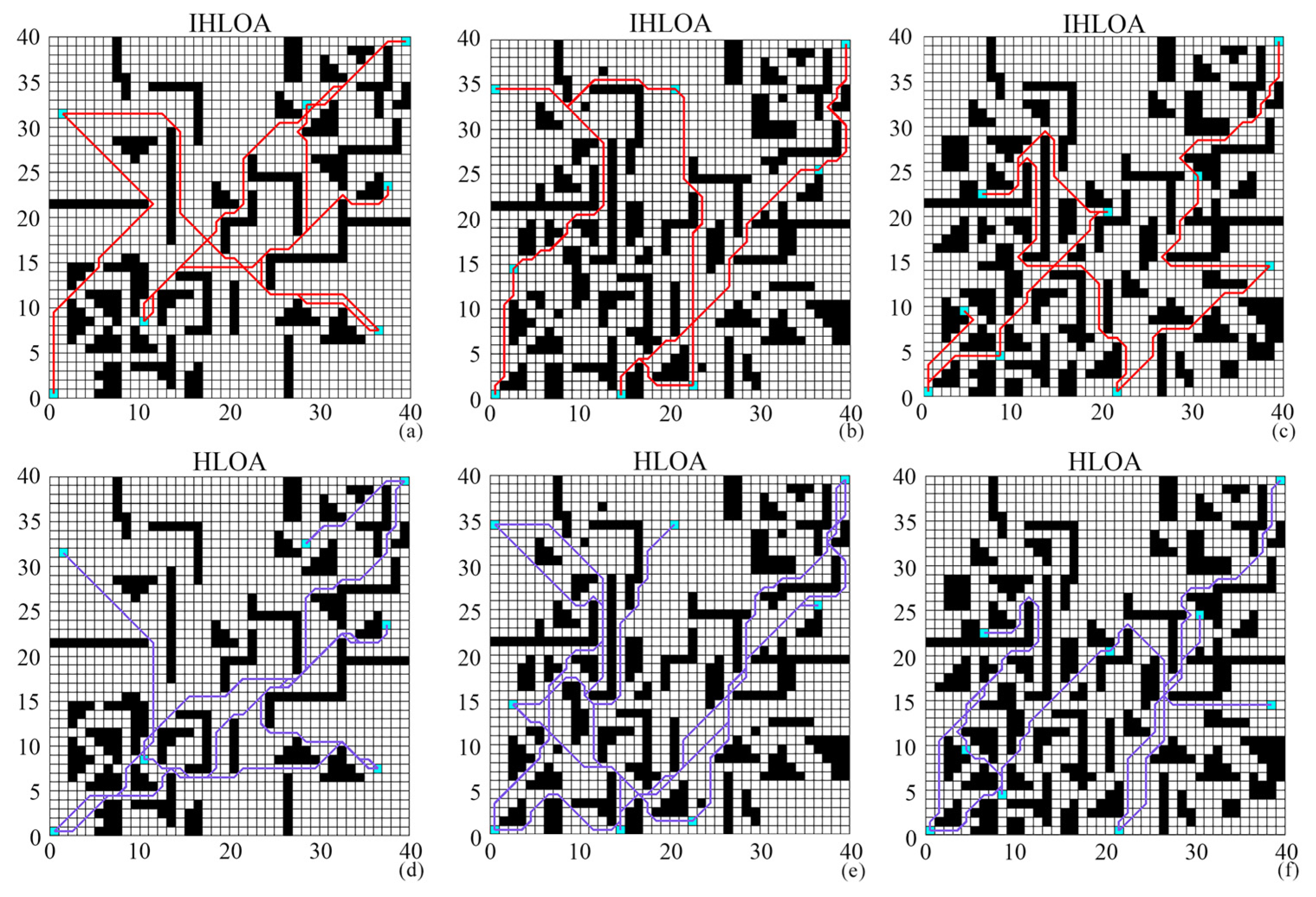
  2. Park, M.H.; Cho, W.S.; Seo, M.K. Hybrid Path Planning Framework to Integrate Improved A*-DWA Algorithms for Enhancing Path Safety and Efficiency. Appl. Ocean Res. 2025, 157, 104497. [Google Scholar] [CrossRef] [Scilit]
  3. Farhangdoust, H.; Wu, M.; Zhou, Z. Coordination Control of Wheeled Mobile Robot Using MPC. In Proceedings of the 7th International Conference on Computational Intelligence, Communication Systems and Networks (CICSyN), Riga, Latvia, 3–5 June 2015. [Google Scholar]
  4. Ge, Y.; Eidsvik, J.; Olaisen, H.J.A. RRT*-Enhanced Long-Horizon Path Planning for AUV Adaptive Sampling Using a Cost Valley. Knowl.-Based Syst. 2025, 315, 113261. [Google Scholar] [CrossRef] [Scilit]
  5. Nhouchi, A.; Said, B.S.; Abdallah, B.A.M.; Aifaoui, N. A Real-Time A* Algorithm for Trajectories Generation and Collision Avoidance in Uncertain Environments for Assembly Applications. Comput. Ind. Eng. 2025, 202, 110959. [Google Scholar] [CrossRef] [Scilit]
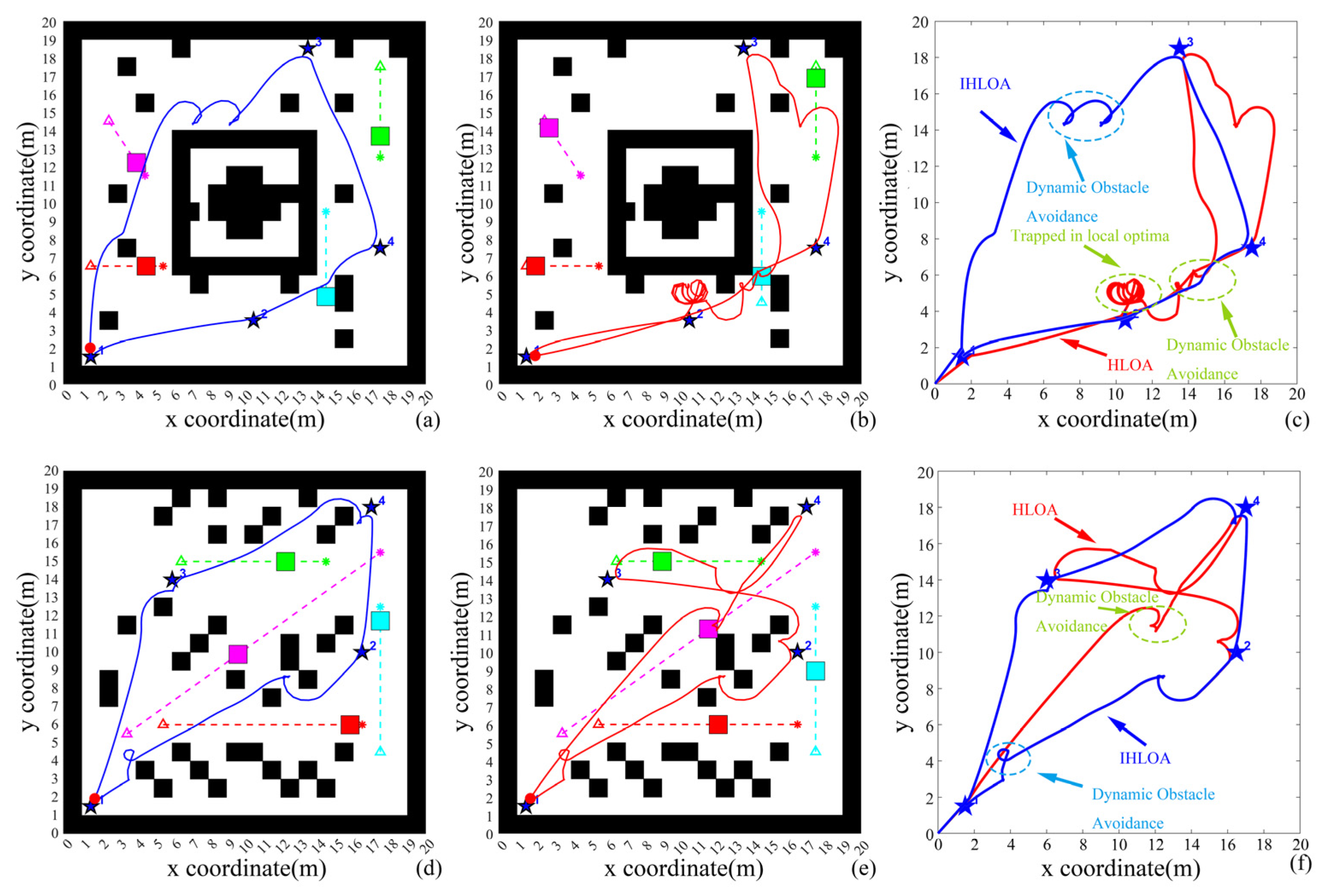
  6. Jin, W.; Li, J.; Lv, X.; Zhang, T. An Optimized Path Planning Approach for Automatic Parking Using Hybrid A* Bidirectional Search. Appl. Intell. 2024, 55, 201. [Google Scholar] [CrossRef] [Scilit]
  7. Liang, J.; Luo, W.; Qin, Y. Path Planning of Multi-Axis Robotic Arm Based on Improved RRT*. Comput. Mater. Contin. 2024, 81, 1009–1027. [Google Scholar] [CrossRef] [Scilit]
  8. Cao, G.; Zhang, B.; Li, Y.; Wang, Z.; Diao, Z.; Zhu, Q.; Liang, Z. Environmental Mapping and Path Planning for Robots in Orchard Based on Traversability Analysis, Improved LeGO-LOAM and RRT* Algorithms. Comput. Electron. Agric. 2025, 230, 109889. [Google Scholar] [CrossRef] [Scilit]
  9. Shen, J.; Fan, J.; Chan, T. Microplastic Sampling Path Planning for Unmanned Surface Vehicle (USV) Based on RRT* and Dijkstra Fusion Algorithm. J. Phys. Conf. Ser. 2024, 2897, 012023. [Google Scholar] [CrossRef] [Scilit]
  10. Wu, S.; Dong, A.; Li, Q.; Wei, W.; Zhang, Y.; Ye, Z. Application of Ant Colony Optimization Algorithm Based on Farthest Point Optimization and Multi-Objective Strategy in Robot Path Planning. Appl. Soft Comput. 2024, 167, 112433. [Google Scholar] [CrossRef] [Scilit]
  11. Cui, J.; Wu, L.; Huang, X.; Xu, D.; Liu, C.; Xiao, W. Multi-Strategy Adaptable Ant Colony Optimization Algorithm and Its Application in Robot Path Planning. Knowl.-Based Syst. 2024, 288, 111459. [Google Scholar] [CrossRef] [Scilit]
  12. Hu, G.; Cheng, M.; Houssein, E.H.; Jia, H. CMPSO: A Novel Co-Evolutionary Multigroup Particle Swarm Optimization for Multi-Mission UAVs Path Planning. Adv. Eng. Inform. 2025, 63, 102923. [Google Scholar] [CrossRef] [Scilit]
  13. Mishra, B.; Sevil, E.H. Path Planning Algorithm Design Using Particle Swarms Optimization and Artificial Potential Fields. Electron. Lett. 2024, 60, e70038. [Google Scholar] [CrossRef] [Scilit]
  14. Wang, Z.; Peng, Q.; Rao, W.; Li, D. An Improved Sparrow Search Algorithm with Multi-Strategy Integration. Sci. Rep. 2025, 15, 3314. [Google Scholar] [CrossRef] [Scilit]
  15. Xu, W.; Hou, C.; Li, G.; Cui, C. Path Planning for Wall-Climbing Robots Using an Improved Sparrow Search Algorithm. Actuators 2024, 13, 370. [Google Scholar] [CrossRef] [Scilit]
  16. Qu, L.; Fan, J. Unmanned Combat Aerial Vehicle Path Planning in Complex Environment Using Multi-Strategy Sparrow Search Algorithm with Double-Layer Coding. J. King Saud Univ. Comput. Inf. Sci. 2024, 36, 102255. [Google Scholar] [CrossRef] [Scilit]
  17. Wang, J.; Wang, W.C.; Hu, X.X.; Qiu, L.; Zang, H.-F. Black-Winged Kite Algorithm: A Nature-Inspired Meta-Heuristic for Solving Benchmark Functions and Engineering Problems. Artif. Intell. Rev. 2024, 57, 98. [Google Scholar] [CrossRef] [Scilit]
  18. Mohamed, A.; Reda, M.; Mohamed, A. Crested Porcupine Optimizer: A New Nature-Inspired Metaheuristic. Knowl.-Based Syst. 2024, 284, 111257. [Google Scholar]
  19. Chen, Z.; Li, S.; Khan, T.A.; Mirjalili, S. Competition of Tribes and Cooperation of Members Algorithm: An Evolutionary Computation Approach for Model Free Optimization. Expert Syst. Appl. 2025, 265, 125908. [Google Scholar] [CrossRef] [Scilit]
  20. Pérez, H.V.; Pardo, A.D.; Torres, M.M.; Morales-Cepeda, A.B.; Sinha, N. A Novel Metaheuristic Inspired by Horned Lizard Defense Tactics. Artif. Intell. Rev. 2024, 57, 59. [Google Scholar] [CrossRef] [Scilit]
  21. Bouteraa, Y.; Khishe, M. Fractal and Chaotic Map-Enhanced Grey Wolf Optimization for Robust Fire Detection in Deep Convolutional Neural Networks. Sci. Rep. 2025, 15, 11495. [Google Scholar] [CrossRef] [Scilit]
  22. Kmich, M.; Ghouate, E.N.; Bencharqui, A.; Karmouni, H.; Sayyouri, M.; Askar, S.; Abouhawwash, M. Chaotic Puma Optimizer Algorithm for Controlling Wheeled Mobile Robots. Eng. Sci. Technol. Int. J. 2025, 63, 101982. [Google Scholar] [CrossRef] [Scilit]
  23. Akhtar, M.M.; Singh, M.; Kadyan, V.; Dua, M. Optimizing Audio Encryption Efficiency: A Novel Framework Using Double DNA Operations and Chaotic Map-Based Techniques. Comput. Electr. Eng. 2025, 123, 110088. [Google Scholar] [CrossRef] [Scilit]
  24. Islam, A.M.; Hassan, R.I.; Ahmed, P. Dynamic Complexity of Fifth-Dimensional Henon Map with Lyapunov Exponent, Permutation Entropy, Bifurcation Patterns and Chaos. J. Comput. Appl. Math. 2025, 466, 116547. [Google Scholar] [CrossRef] [Scilit]
  25. Wang, R.; Deng, G.Q.; Deng, X.F. An Image Encryption Scheme Based on Double Chaotic Cyclic Shift and Josephus Problem. J. Inf. Secur. Appl. 2021, 58, 102699. [Google Scholar] [CrossRef] [Scilit]
  26. Tanyildizi, E.; Demir, G. Golden Sine Algorithm: A Novel Math-Inspired Algorithm. Adv. Electr. Comput. Eng. 2017, 17, 71–78. [Google Scholar] [CrossRef] [Scilit]
  27. Xiao, Z.Y.; Liu, S. Study on Elite Opposition-Based Golden-Sine Whale Optimization Algorithm and Its Application of Project Optimization. Acta Electron. Sin. 2019, 47, 2177–2186. [Google Scholar]
  28. Majumdar, P.; Mitra, S. Enhanced Honey Badger Algorithm Based on Nonlinear Adaptive Weight and Golden Sine Operator. Neural Comput. Appl. 2024, 37, 367–386. [Google Scholar] [CrossRef] [Scilit]
  29. Meng, A.; Rong, J.; Yin, H.; Luo, J.; Tang, Y.; Zhang, H.; Li, C.; Zhu, J.; Yin, Y.; Li, H.; et al. Solving Large-Scale Combined Heat and Power Economic Dispatch Problems by Using Deep Reinforcement Learning Based Crisscross Optimization Algorithm. Appl. Therm. Eng. 2024, 245, 122781. [Google Scholar] [CrossRef] [Scilit]
  30. Meng, A.; Xu, X.; Zhang, Z.; Zeng, C.; Liang, R.; Zhang, Z.; Wang, X.; Yan, B.; Yin, H.; Luo, J. Solving High-Dimensional Multi-Area Economic Dispatch Problem by Decoupled Distributed Crisscross Optimization Algorithm with Population Cross Generation Strategy. Energy 2022, 258, 124836. [Google Scholar]
  31. Wang, S.; Tang, W.; Ou, B.; Pan, J.S. Reversible Data Hiding Method for Multi-Histogram Point Selection Based on Improved Crisscross Optimization Algorithm. Inf. Sci. 2021, 549, 13–33. [Google Scholar] [CrossRef] [Scilit]
  32. Meng, A.; Ge, J.; Yin, H.; Chen, S. Wind Speed Forecasting Based on Wavelet Packet Decomposition and Artificial Neural Networks Trained by Crisscross Optimization Algorithm. Energy Convers. Manag. 2016, 114, 75. [Google Scholar] [CrossRef] [Scilit]
Figure 1. The flowchart of the IHLOA.
Algorithms 19 00272 g001
Figure 2. Convergence curves of the IHLOA with different r1 values on benchmark functions. Subfigures (au) are the convergence curves of each benchmark function.
Algorithms 19 00272 g002
Figure 3. Convergence curves of the IHLOA with different r2 values on benchmark functions. Subfigures (au) are the convergence curves of each benchmark function.
Algorithms 19 00272 g003
Figure 4. Convergence curves of the IHLOA with different pc values on benchmark functions. Subfigures (au) are the convergence curves of each benchmark function.
Algorithms 19 00272 g004
Figure 5. Radar charts and average ranking for the IHLOA parameter sensitivity analysis. (ac) Radar plots of each benchmark function for r1, r2, and pc, respectively. Subfigures (df) Show average rankings of each algorithm.
Algorithms 19 00272 g005
Figure 6. Convergence curves of the IHLOA and its strategy ablation variants on benchmark functions. Subfigures (au) show convergence curves of different benchmark functions under various algorithms.
Algorithms 19 00272 g006
Figure 7. Convergence curves of the IHLOA and comparative algorithms on benchmark functions. Subfigures (au) are the convergence curves of each benchmark function under different algorithms.
Algorithms 19 00272 g007
Figure 8. Radar charts and average ranking for the IHLOA and comparative algorithms. Subfigures (ac) show radar plots of each benchmark function; subfigures (df) show average rankings of each algorithm.
Algorithms 19 00272 g008
Figure 9. Box plots of the IHLOA and comparative algorithms. Subfigures (au) are the box plots of each benchmark function under different algorithms.
Algorithms 19 00272 g009
Figure 10. Block diagram for path planning experiment.
Algorithms 19 00272 g010
Figure 11. Path planning trajectories and convergence curves of each algorithm on single-objective grid maps with different scales: (a) path planning trajectory on 20 × 20 grid map; (b) path planning trajectory on 25 × 25 grid map; (c) path planning trajectory on 30 × 30 grid map; (d) convergence curve on 20 × 20 grid map; (e) convergence curve on 25 × 25 grid map; (f) convergence curve on 30 × 30 grid map.
Algorithms 19 00272 g011
Figure 12. Distribution of multiple goal points. Subgraphs (a,d,g) show goal point distributions in 20 × 20 path planning with obstacle rates of 0.2, 0.25, and 0.3. Subgraphs (b,e,h) present distributions in 30 × 30 grids under the same rates. Subgraphs (c,f,i) depict distributions in 40 × 40 grids with the same obstacle rates.
Algorithms 19 00272 g012
Figure 13. Path planning in a 20 × 20 grid. Subgraphs (a,d) correspond to the path planning results of the IHLOA and the HLOA, respectively, under an obstacle rate of 0.2. Subgraphs (b,e) present the same scenario with an obstacle rate of 0.25. Subgraphs (c,f) show the results under an obstacle rate of 0.3.
Algorithms 19 00272 g013
Figure 14. Path planning in a 30 × 30 grid. Subgraphs (a,d) correspond to the path planning results of the IHLOA and the HLOA, respectively, under an obstacle rate of 0.2. Subgraphs (b,e) present the same scenario with an obstacle rate of 0.25. Subgraphs (c,f) show the results under an obstacle rate of 0.3.
Algorithms 19 00272 g014
Figure 15. Path planning in a 40 × 40 grid. Subgraphs (a,d) correspond to the path planning results of the IHLOA and the HLOA, respectively, under an obstacle rate of 0.2. Subgraphs (b,e) present the same scenario with an obstacle rate of 0.25. Subgraphs (c,f) show the results under an obstacle rate of 0.3.
Algorithms 19 00272 g015
Figure 16. Simulation results of dynamic multi-goal path planning: (a) the HLOA’s path on Map 1; (b) the IHLOA’s path on Map 1; (c) dynamic obstacle avoidance trajectory of Map 1; (d) the HLOA’s path on Map 2; (e) the IHLOA’s path on Map 2; (f) dynamic obstacle avoidance trajectory of Map 2.
Algorithms 19 00272 g016
Table 1. Setting the parameters of the IHLOA and its comparison algorithms.
AlgorithmParameterValueAlgorithmParameterValue
IHLOAr10.5πGOOSEalphaDecreased from 2 to 0
r20.5πs_s343.2
pc0.5ACOq0.5
Delta2 zeta1.0
HLOADelta2SSDCorrection factor2.0
Inertia coefficient1.0
PSOw0.7ESCa0.15
c11.2b0.35
c21.2beta_base1.5
HBODegree3Mask_probability0.5
eGSKKR1
K10
Note: The italic parameters in this table represent the adaptive/key control parameters of the corresponding algorithms.
Table 2. Path planning simulation parameters.
Simulation Control ParametersDynamic Obstacle Avoidance Parameters
ParameterValueParameterValue
Max_steps8000Dwa_params.max_v0.9 m/s
Goal_threshold0.8 mDwa_params.max_w100π/180 rad/s
Stuck_threshold0.5 mDwa_params.max_accel0.3 m/s2
Stuck_check_window80Dwa_params.max_dyaw100π/180 rad/s2
Replan_cooldown100 StepsDwa_params.clearance_weight0.3
Max_replan_attempts3Dwa_params.velocity_weight0.15
Table 3. Algorithm performance on multi-scale single-objective grid maps.
MapIndexIHLOAHLOAHBOeGSKESCPSO
20 × 20Minimum path length (m)28.83230.447.144.1129.70
Path length reduction (%) −11.11%−5.51%−63.63%−53.34%−3.24%
Number of turning points9129181113
Turning points reduction (%) −33.33%−0.00%−100.00%−22.22%−44.44%
25 × 25Minimum path length (m)38.788656.970644.126345.458672.783156.4268
Path length reduction (%) −46.87%−13.76%−17.20%−87.64%−45.47%
Number of turning points121316162019
Turning points reduction (%) −8.33%−33.33%−33.33%−66.67%−58.33%
30 × 30Minimum path length (m)47.279170.037548.478269.11687.66451.851
Path length reduction (%) −48.14%−2.54%−46.19%−85.42%−9.67%
Number of turning points111812162315
Turning points reduction (%) −63.64%−9.09%−45.45%−109.09%−36.36%
Table 4. Comparison of shortest path lengths between the IHLOA and the HLOA in diverse scenarios.
MapObstacle RateMinimum Path Length (IHLOA)/mMinimum Path Length (HLOA)/mPath Length Decrease (%)
20 × 200.253.9411357.11275.55
20 × 200.2574.1837775.11271.24
20 × 200.390.6690592.154331.61
20 × 20 (Avg)72.9313274.793242.80
30 × 300.2111.6396114.4682.47
30 × 300.25128.6102128.78170.13
30 × 300.3143.9828149.4683.67
30 × 30 (Avg)128.0775130.90592.09
40 × 400.2153.9239156.1961.45
40 × 400.25173.5391178.78172.93
40 × 400.3164.4092178.68127.99
40 × 40 (Avg)163.9574171.21974.12
Overall (Avg)121.6554125.63963.00
Note: The bold values in the “Path Length Decrease (%)” column denote the percentage reduction in path length achieved by the proposed IHLOA algorithm relative to the HLOA, emphasizing its superior optimization performance in diverse scenarios.
Table 5. Comparison of traversal order and turning points between the IHLOA and the HLOA in diverse scenarios.
MapObstacle RateTraversal Order (IHLOA)Traversal Order (HLOA)Number of Turning Points (IHLOA)Number of Turning Points (HLOA)Reduction in Turning Points (%)
20 × 200.2[1, 6, 2, 4, 3, 5, 7][1, 6, 2, 5, 3, 4, 7]23244.17
0.25[1, 2, 4, 5, 8, 7, 6, 3][1, 2, 6, 3, 7, 4, 5, 8]15166.25
0.3[1, 4, 3, 2, 5, 6, 8, 7, 9][1, 7, 8, 3, 5, 9, 4, 6, 2]293517.14
20 × 20 (Avg)22.3325.0010.85
30 × 300.2[1, 2, 3, 4, 6, 5, 7][1, 7, 3, 2, 6, 5, 4]45450.00
0.25[1, 6, 5, 4, 7, 3, 8, 2][6, 1, 5, 3, 8, 4, 7, 2]33342.94
0.3[2, 4, 1, 7, 8, 3, 5, 9, 6][6, 1, 2, 5, 7, 8, 4, 3, 9]57605.00
30 × 30 (Avg)45.0046.332.65
40 × 400.2[1, 5, 2, 6, 7, 3, 4][6, 7, 1, 3, 2, 4, 5]446229.03
0.25[1, 4, 6, 7, 3, 2, 5, 8][7, 4, 3, 8, 1, 6, 2, 5]638021.25
0.3[4, 1, 3, 6, 7, 2, 5, 8, 9][9, 2, 8, 5, 6, 1, 7, 4, 3]566716.42
40 × 40 (Avg)54.3369.6722.23
Overall (Avg)40.5647.0011.91
Note: The bold values in the “Reduction in Turning Points (%)” column denote the percentage reduction in the number of turning points achieved by the proposed IHLOA algorithm relative to the HLOA, emphasizing its superior performance in generating smoother paths with fewer directional changes.
Table 6. Comparison of performance indicators for dynamic path planning.
IndicatorHLOAIHLOAHLOA vs. IHLOA
Map 1Total length of path (m)241.3854.87Shortened by 77.3%
Total simulation steps30651384Shortened by 54.9%
Running time (s)306.5138.4Shortened by 54.9%
Actual trajectory length91.79 58.78Shortened by 36.0%
Number of robot stuck times135Shortened by 61.5%
Number of replanning failures00No failure
Map 2Total length of path (m)69.1556.53Shortened by 18.2%
Total simulation steps19261463Shortened by 24.0%
Running time (s)192.6146.3Shortened by 24.0%
Actual trajectory length81.8661.65Shortened by 24.7%
Number of robot stuck times54Shortened by 20.0%
Number of replanning failures00No failure
Disclaimer/Publisher’s Note: The statements, opinions and data contained in all publications are solely those of the individual author(s) and contributor(s) and not of MDPI and/or the editor(s). MDPI and/or the editor(s) disclaim responsibility for any injury to people or property resulting from any ideas, methods, instructions or products referred to in the content.