An Explanatory CDF Manifold Algorithm for Large Telecom Datasets

Abstract

In this paper we introduce the CDF manifold algorithm, which operates on datasets where a single target dimension is strictly increasing given a minimum of two or more input dimensions, which is very common in telco data. The manifold can then be used to compute the closest upper and lower limits to a given new point, as well as its CDF. Training takes $O(n.ln[n\left]\right)$ steps in the best case and $O\left(n^{3/2}\right)$ in the worst case. Lookup takes $O\left(ln\right[n\left]\right)$ steps in the best case and $O(n^{1/2}ln\left(n\right))$ in the worst case. The asymptotic computational cost is proven with a theorem. We compare our manifold method versus a standard dense neural network and show the asymptotic advantages both in terms of speed and accuracy. We also address potential speed gains through the use of reference points. In summary, the manifold is a non-parametric explanatory method to find the tightest data-driven upper and lower limits of the output dimension given a new unseen input. This makes it ideal for planning new site deployments where we need to find actual measurements as a baseline performance.

1. Introduction

Manifold methods [1] comprise an active area of research and have found applications as dimensionality reduction techniques [2], in representation learning [3] or just for data exploration. Broadly speaking, the algorithms fall into a number of categories, namely probability manifolds [4], neural network (NN) manifolds [5], geometric manifolds [6,7] and graph manifolds [8]. However, the sheer number of possible manifolds that exist in nature and the possible ways to detect them are so innumerable that the general consensus on what algorithms are expected to work best comes from a prior understanding of the physical system that created the manifold. Because of that, the algorithms in this paper are mostly based on the following observation: the physical laws that underlie most telecom data mandate a strictly increasing manifold.

For example, increasing only the Signal-to-Noise Ratio (SNR) for single users and keeping all the other variables the same is guaranteed to worsen the cell throughput. Similarly, if the type of service even for a single user needs more bit rate, this is also guaranteed to worsen the cell throughput. Furthermore, if we increase any combination of these variables, then the cell throughput will decrease. This means the variables and the cell throughput lie on a strictly increasing manifold.

Let us call that manifold a CDF manifold because the CDF is always a strictly increasing manifold and there is a relation between computing the high-dimensional CDF and computing the corresponding value of the telecom data that lie on such a manifold.

If we try to apply any of the standard manifold methods, for example, NN, then we would struggle to regularize it, while the training costs for large datasets will be high. On the other hand it is practically impossible to force the NN to adhere to the strictly increasing property of the data. Therefore, an attentive customer would ask why the NN is inferring that, if the activity on a cell increases while the rest of the KPIs remain the same, the cell throughput will improve. The simple reality of the situation is that there might be a better non-parametric method to model the data, and to this end we propose the CDF manifold algorithm.

We say that any telco data that has the strictly increasing property has the CDF manifold property. Such data admits the specialized set of constructions we define in Section 2, where, by Theorem 1, the manifold is constructed in $O\left(n^{3/2}\right)$ steps in the worst case and in $O(n.ln[n\left]\right)$ steps in the best case. The manifold allows two additional specialized constructions that build on previous work in [9], enabling binary searches that cost $O\left(ln\right[n\left]\right)$ in the best case and $O\left(n^{1/2}ln\left[n\right]\right)$ in the worst case. Furthermore, the manifold we propose in this paper has the important property that it also allows us to compute the CDF once the manifold is constructed, as described in Section 4, which gives the manifold its name. In Section 3 we outline the necessary pseudocode to implement the CDF manifold. Last but not least we perform a comparative simulation between an NN and the CDF manifold in Section 5.

2. Defining the Manifold, Properties and Sampling

To formalize the aforementioned pattern, assume we have data $[x_1,x_2,\dots ,x_k\dots x_d]$ in d dimensions and a target single dimension y of the data such that, if any $x_k$ increases independently of any other x, then y stays the same or increases. Therefore, if $y=CD{F}_{manifold}[x_1,x_2\dots x_k,\dots x_d]$ and $[v_1,v_2,\dots ,v_k\dots v_d],v_k\ge 0\forall k$, then $y=CD{F}_{manifold}[x_1,x_2\dots x_k,\dots x_d]\le CD{F}_{manifold}[x_1+v_1,x_2+v_1\dots x_k+v_k,\dots x_d+v_d]$. The pseudocode for this comparison is given in Algorithm 1.

To simplify the notations and proofs, we consider the manifold in 2D, which is also the smallest whole number of dimensions where the manifold method is valid. Therefore, for the remainder of the paper, consider two-dimensional data $[x_1,x_2]$ and $y=CD{F}_{manif}[x_1,x_2]$.

Next assume we have 2 data points $[a_1,a_2]$ mapping to $y_a=CD{F}_{manif}[a_1,a_2]$ and $[b_1,b_2]$ mapping to $y_b=CD{F}_{manif}[b_1,b_2]$ such that $[a_1<b_1,a_2<b_2]$, which also means that $y_a<y_b$. Also assume we have a new input data point $[g_1,g_2]$ for which we want to compute $y_g$. Because we know the data lies on a CDF manifold, we know that, if $a_1<g_1<b_1$ and $a_2<g_2<b_2$, then $y_a<y_g<y_b$. Therefore, if $[a,b]$ is the tightest for g in the data, then we can compute $y_g=(y_a+y_b)/2$. Observe that this estimate is a data-driven explanatory computation since we can explain $y_a,y_b$, which is not true for NN, for example. This means that, if the customer asks why we made a given inference, we can point out the actual data measurements we used, while, with the NN, we will not be able to give a definitive answer.

The drawback of this CDF estimate is that we must have as much data as possible to make sure that the interval is as tight as possible. As a result the lookup algorithm must be extremely efficient computationally and use as little memory as possible. For instance, for large data, even $O\left(n^2\right)$ complexity becomes infeasible, so we set out to look for an algorithm that is more efficient.

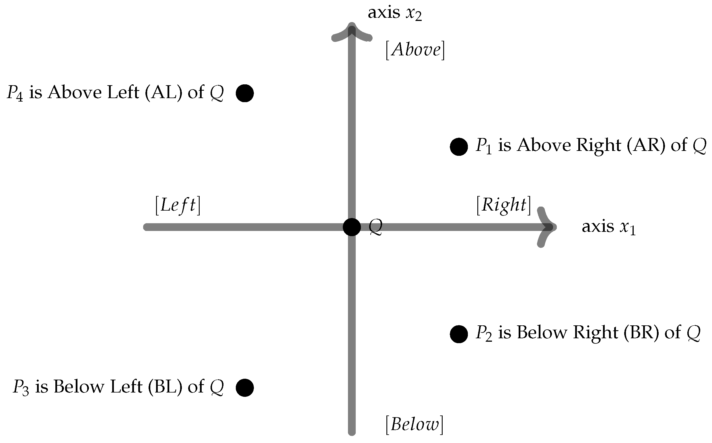
Next, a point b is considered above right (AR) of point a if $a_1<b_1$ and $a_2<b_2$. Similarly, a point b is considered below left (BL) of point a if $a_1>b_1$ and $a_2>b_2$. Examples of this are given in Figure 1. To further simplify the algorithms observe that computing the below left is equivalent to computing above right but with the necessity of multiplying each data dimension $x_k$ other than the target dimension y by $(-1)$. That is why, for the remainder of the paper, we only consider the algorithms in the context of computing the upper limit (UL) in the AR.

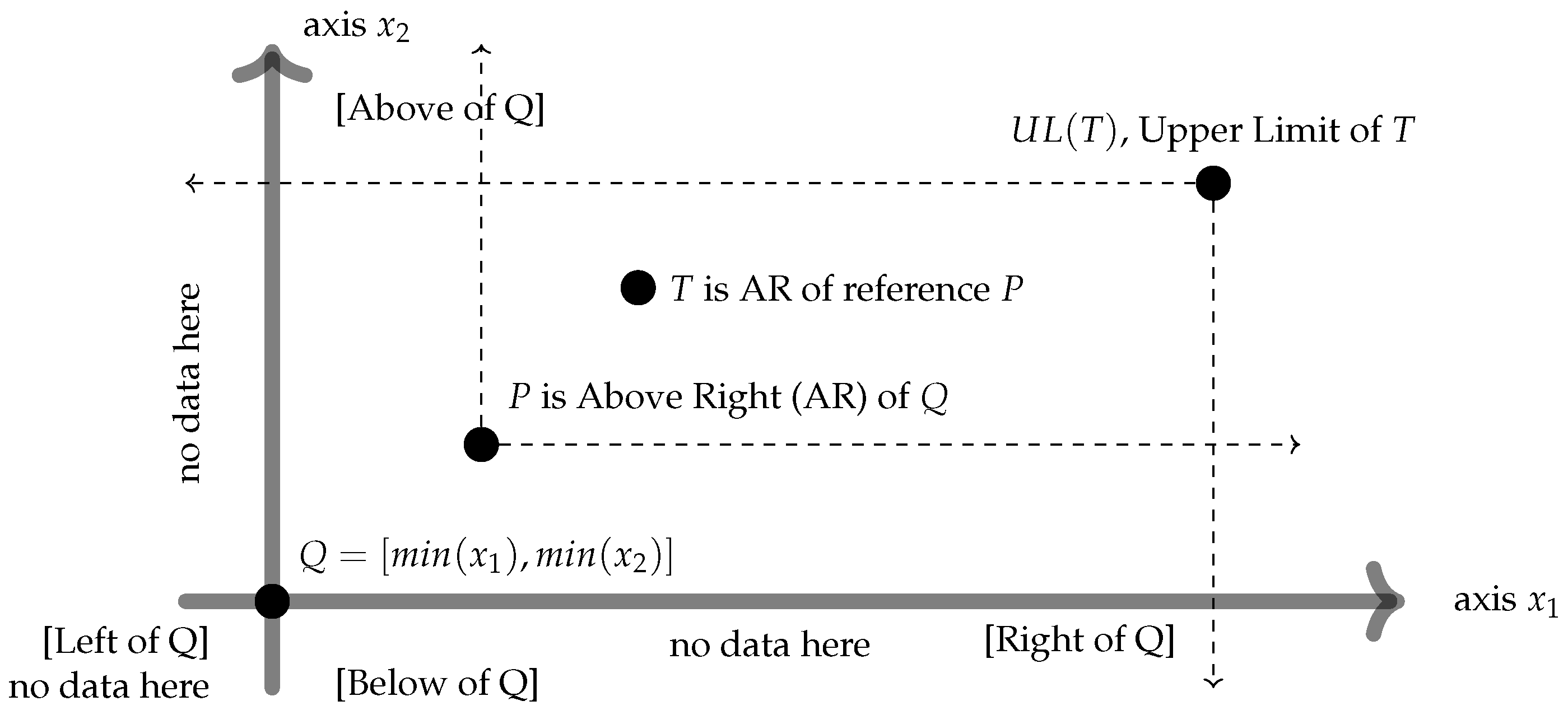
Next, in Figure 2, we show that the AR preserves the upper limit. If a target point T is AR of sample point P then the upper limit of T is also AR of P.

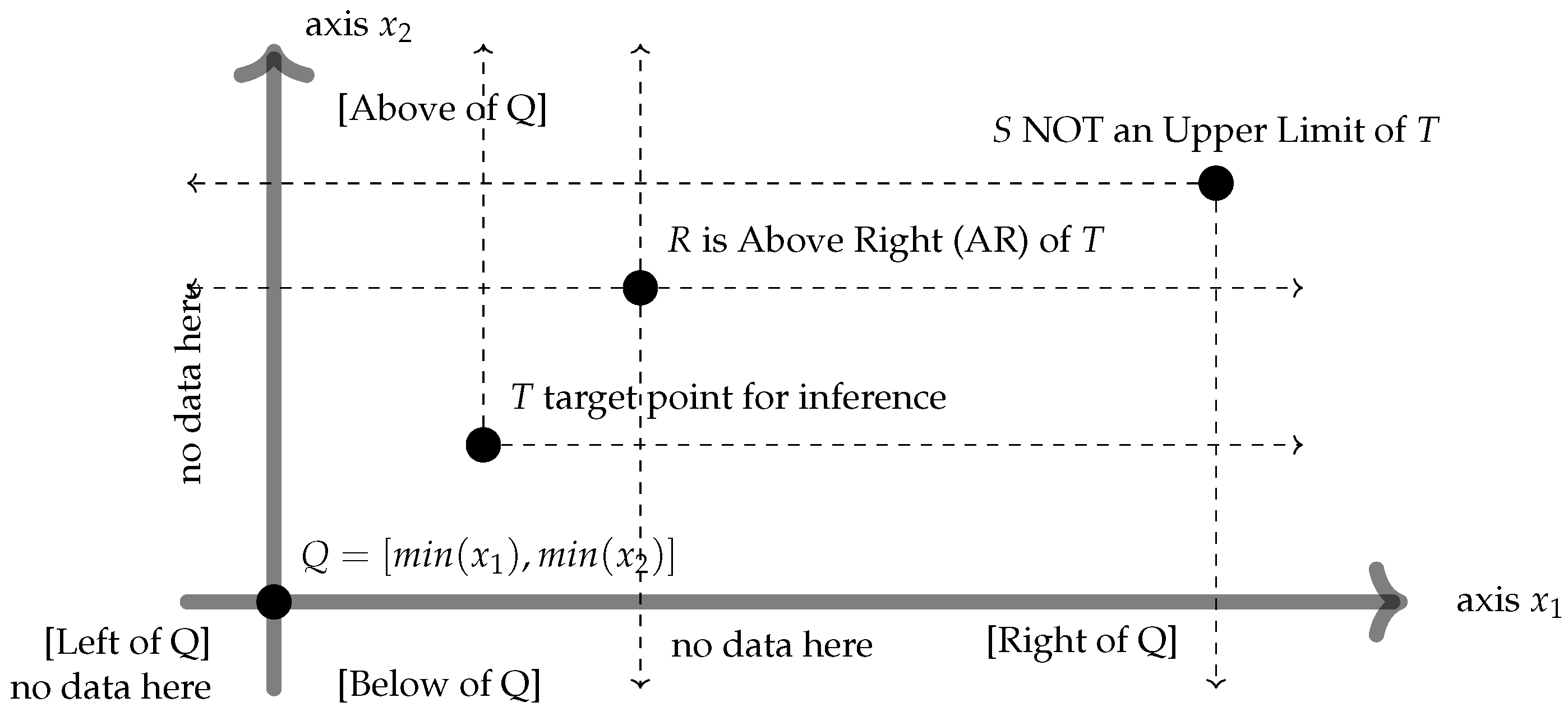
Using the definitions of Figure 1 and the result of Figure 2 we can see that, if we have found a point R that is AR of target point T, then no point that is AR of R like S can ever be a better upper limit to T, as shown in Figure 3. In other words the BL and AR of a reference point R partition the data space such that no point BL of R can have an upper limit in the AR of R.

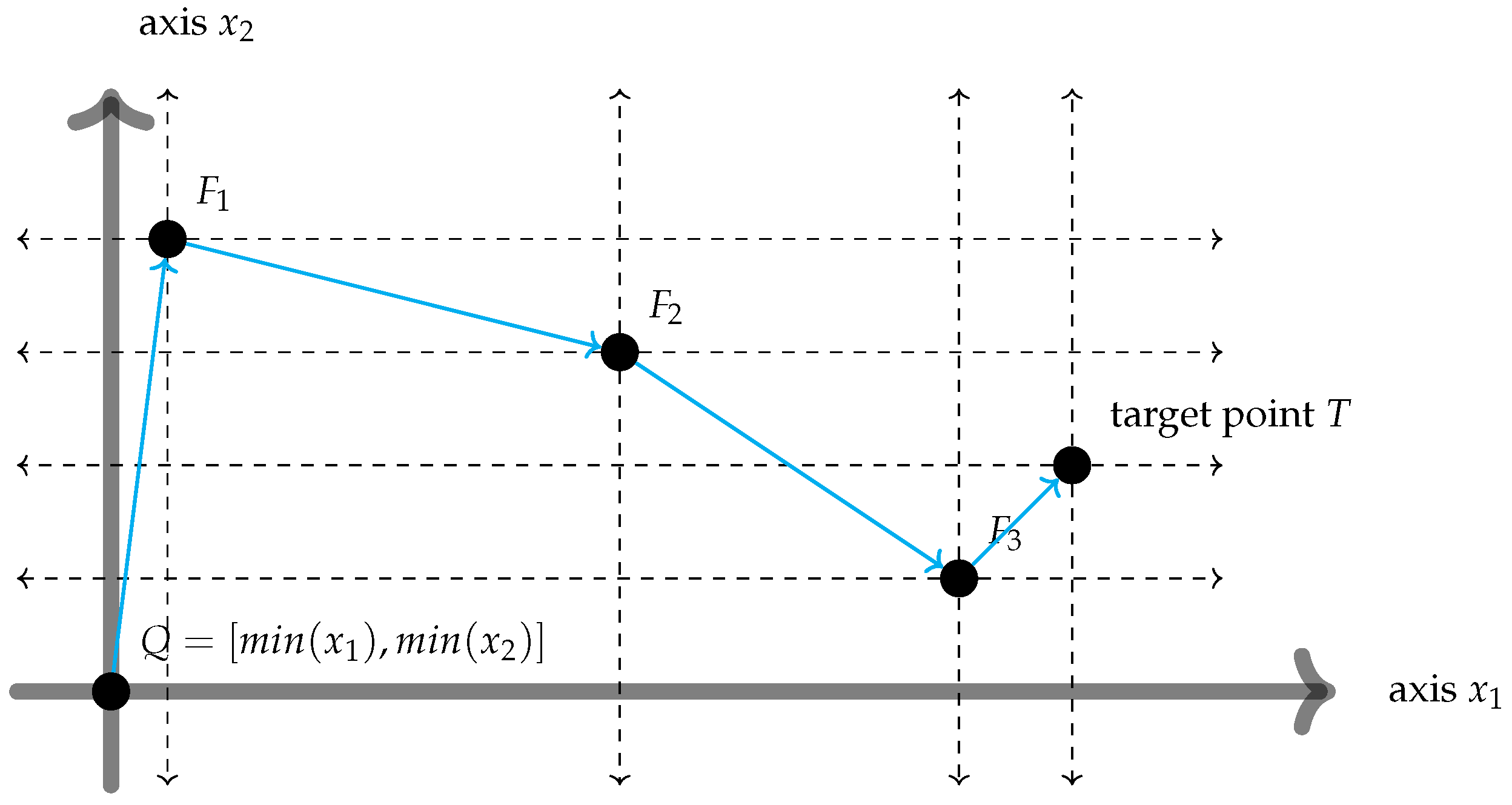
Next consider Figure 4. We define the points $F_1$, $F_2$, $F_3$ to form on a long front, meaning no $F_i$ is AR of $F_j$ for all pairs $[i,j]$. Assume we start the binary search at $F_1$ and T is not AR of $F_1$. Which would be the next check point? In the worst case we might need to check $F_2$ and then $F_3$, and in this case we would do a linear search to $F_3$, at which point we would have found the target point. This proves by example that the AR and BL functions do not eliminate with a single check a portion of the search data in general, which hinders their use for binary searches.

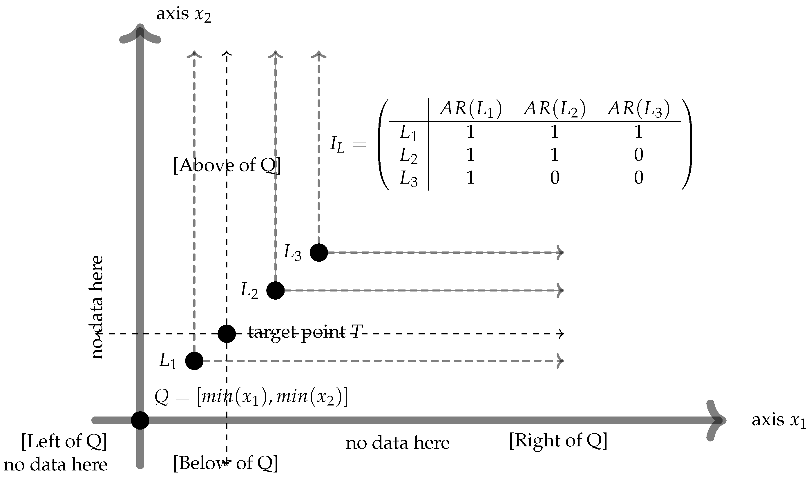
Fortunately there are cases where the AR and BL do reduce the search space with a single check, as depicted in Figure 5. The first structure that supports binary searches is given in Figure 5, where all points L are such that, for any pair $[i,j]$, either $L_i\in AR\left(L_j\right)$ or $L_i\in BL\left(L_j\right)$. We call such points a long line, and we can model their relationship using the Index Invariant Graph (IIG) defined in [9,10]. The incidence matrix $I_L$ defined by the AR operations is clearly a triangular matrix, and, as proven in [9], the dual hypergraph defined by that matrix is isomorphic to the original graph. In this context the dual isomorphism means that the AR operations uniquely describe the location of each data point. As an example consider in Figure 5 the lookup procedure for the target T among the L points. First we could check if T is AR of $L_2$. As a result we would know that T is not AR of any point AR of $L_2$, and therefore we instantly rule out $L_3$ as an upper limit in this case. This means we have eliminated half of the data and can consider the subset that is BL of $L_2$, which would be $L_1$.

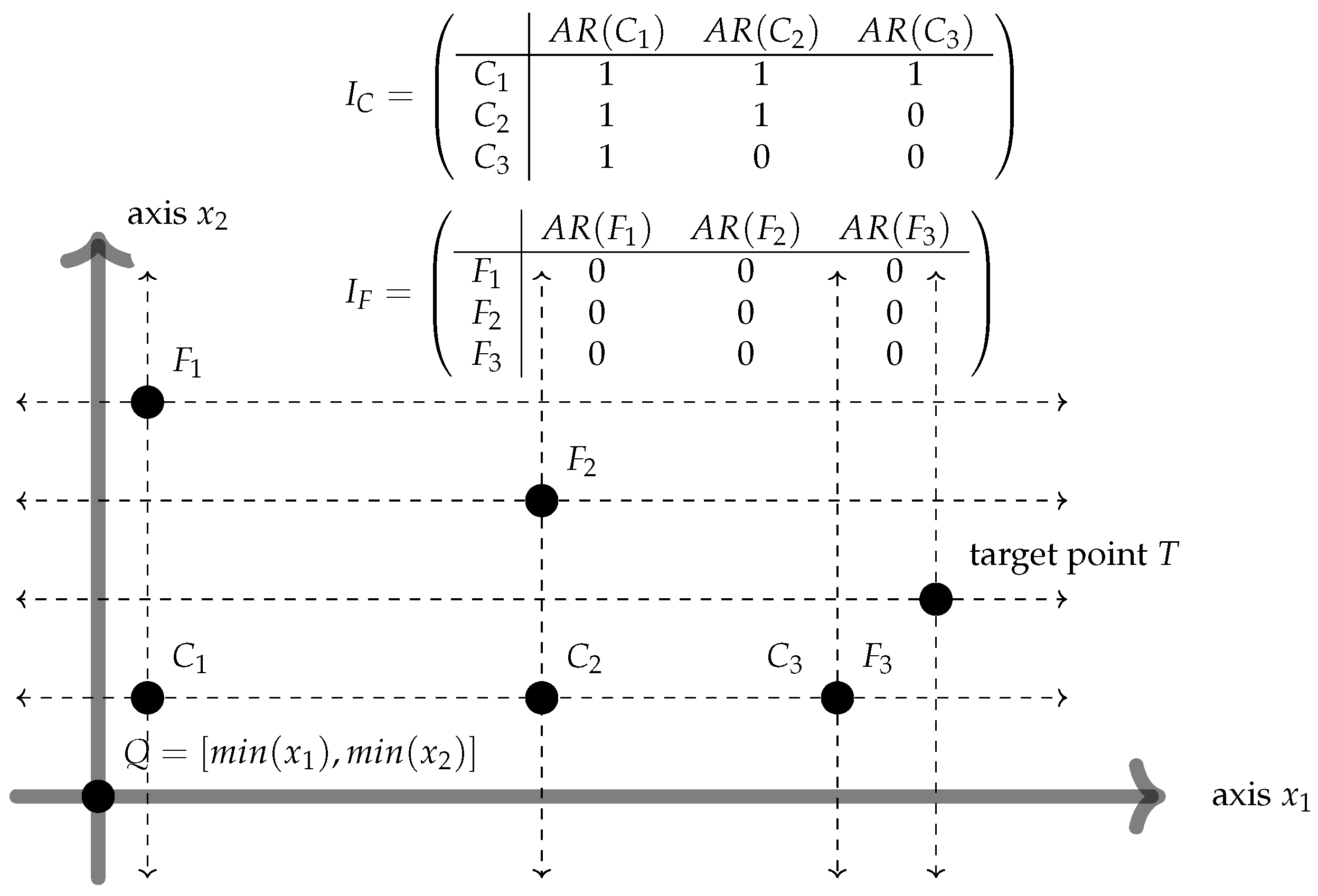
Next, in Figure 6, we apply a similar logic to a different structure. Let us call a long front a structure of points such that all pairs $[i,j]$ are such that $F_i\notin AR\left(F_j\right),F_i\notin BL\left(F_j\right)$. Set $x_1$ as the initial binary search dimension and $x_2$ as a secondary data dimension. Then define the construction of points C such that $C_i$ is a translation of $F_i$ among the secondary data dimension $x_2$ to the minimum value among all data, while the initial binary search dimension $x_1$ is kept constant, or, more explicitly, $C_i=[F_i\left(x_1\right),\{mi{n}_i{F}_i\left(x_2\right)\}]$. Observe that the incidence matrix $I_F$ of the long front is all zeros, while the incidence matrix $I_C$ of the translated data is again modeled with the IIG. As a result we can treat the C points as L. That being said the F points still cannot be treated as L points. Instead a binary search on the C points will return just the closest upper value $best\left(x_1\right)$ along the binary search dimension $x_1$. Once we have the best upper limit $best\left(x_1\right)$ across $x_1$ we must run another binary search among a different data dimension, for example, $x_3$, starting at $best\left(x_1\right)$. We repeat the searches until there are no more dimensions or no more points left to search.

The next question we consider is how we detect the long fronts and lines. Let $data$ be a matrix with n rows and d dimensions. Using Matlab/Octave notation $data(:,k)$ is a single data dimension, and $data(i,:)$ would be a single data instance as a row vector. In this context a regular sort would then be applied to $data(:,k)$, while a dictionary sort would be applied to $data$. A dictionary sort of this type is implemented in [11] and is given in Algorithm 2. Therefore a dictionary sort would order the data in such a way that, if $data(i,:)$ appears before $data(j,:)$, then $data(i,k)\le data(j,k)$ (see Algorithm 1). As a result we can scan the data from i to j and find the next point after i that is part of a long line L after i but before j. Or, more generally, if we do a linear scan we are guaranteed to find the longest line that starts with the first row of the data. Importantly the same linear scan will also give us the longest front that starts with the first row of the dictionary.

In short, to detect a single line or front, we just start at the first row in the sorted dictionary $data(1,:)$ and scan the data linearly until the end $i=1:n$. We maintain two separate queues for the front $q_F$ or line $q_L$, where initially $q_F=data(1,:)$ and $q_L=data(1,:)$. Once we encounter a point i that is in a line with the last point in the line queue we add it to the queue $q_L=[q_L;data(i,:)]$ and mark it as the new end of the line. Similarly, if point i is in a front with the last point in the front queue, we add it to the queue $q_F=[q_F;data(i,:)]$ and mark it as the new end of the front. By the end of the scan either queue will have a long front or a line, meaning a single IIG detection takes $O\left(n\right)$ iterations. The pseudocode for this procedure is given in Algorithm 3.

There is a way to speed up the expensive linear scan $O\left(n\right)$ of a single IIG detection by observing another property of the dictionary sort. This property is best explained with a numeric example, so let us have the following dictionary-sorted data points $d_1=[1,1],d_2=[1,2],d_3=[2,1],d_4=[2,2],d_5=[3,1],d_6=[3,2]$. In this order $d_1\to d_2$ form a line, and, in $d_2\to d_3$, we have an inversion to a front. Similarly $d_3\to d_4$ are a line and $d_4\to d_5$ are an inversion to a front. Therefore, if we start the detection at $d_1$, we would expect the longest line to end at the first inversion, while the front points would likely all be within the inversion. Of course, this approach is just a heuristic, and, in the worst case, we would still need to perform a linear scan.

The next question involves finding the shortest line or front that exists in any dataset. For starters any dataset containing at least 2 points will have the 2 points in a long line of length 2 or a long front of length 2. Let us denote this with $ANY\left[2p\right]=OR[2L,2F]$. If the data has 3 points we would express this as $ANY\left[3p\right]=ANY\left[2p\right]+ANY\left[1p\right]=OR[2L,2F]+ANY\left[1p\right]$. For these functions we can prove that

Theorem 1.

$$ANY\left[n^{2}p\right]=OR\left[nL,nF\right]+ANY\left[(n^2-n)p\right]$$

(1)

meaning that, in a dataset of size n, the shortest long front or long line contains $n^{1/2}$ points.

Proof of Theorem 1. 

We prove Theorem 1 by induction. To start the induction we already showed that Equation (1) is true for any 2 data points. Next, we assume it is true up to some number n. For the induction step we need to prove it is true for $n+1$, or, more explicitly, that

$$ANY\left[{(n+1)}^{2}p\right]=OR\left[(n+1)L,(n+1)F\right]+ANY\left[({(n+1)}^2-(n+1))p\right]$$

(2)

The left side of Equation (2) can be rewritten as $ANY\left[{(n+1)}^{2}p\right]=ANY\left[n^{2}p\right]+ANY\left[({(n+1)}^2-n^2)p\right]$ and by Equation (1) we know that $ANY\left[n^{2}p\right]$ contains $OR\left[nL,nF\right]$ giving:

$$ANY\left[{(n+1)}^{2}p\right]=OR\left[nL,nF\right]+ANY\left[({(n+1)}^2-n)p\right]$$

(3)

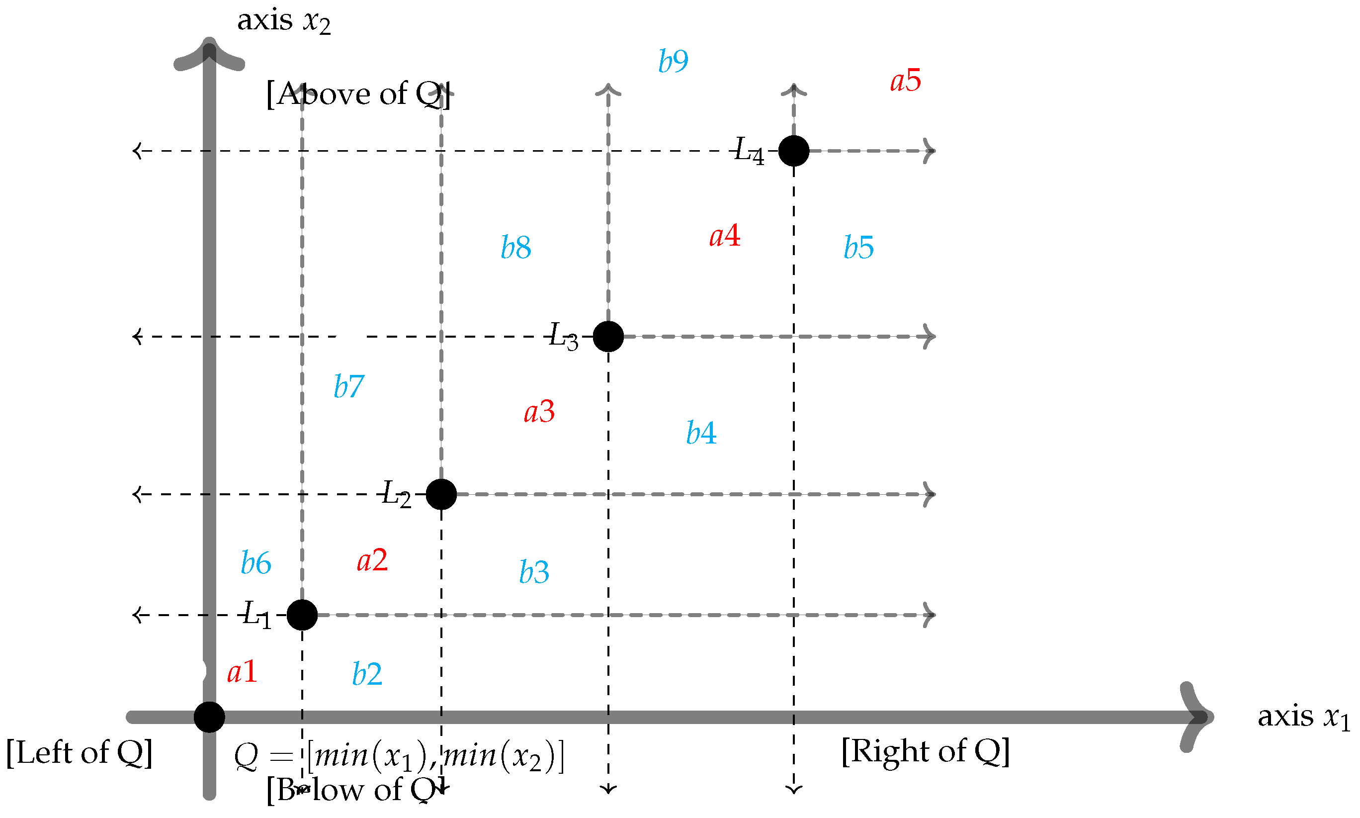
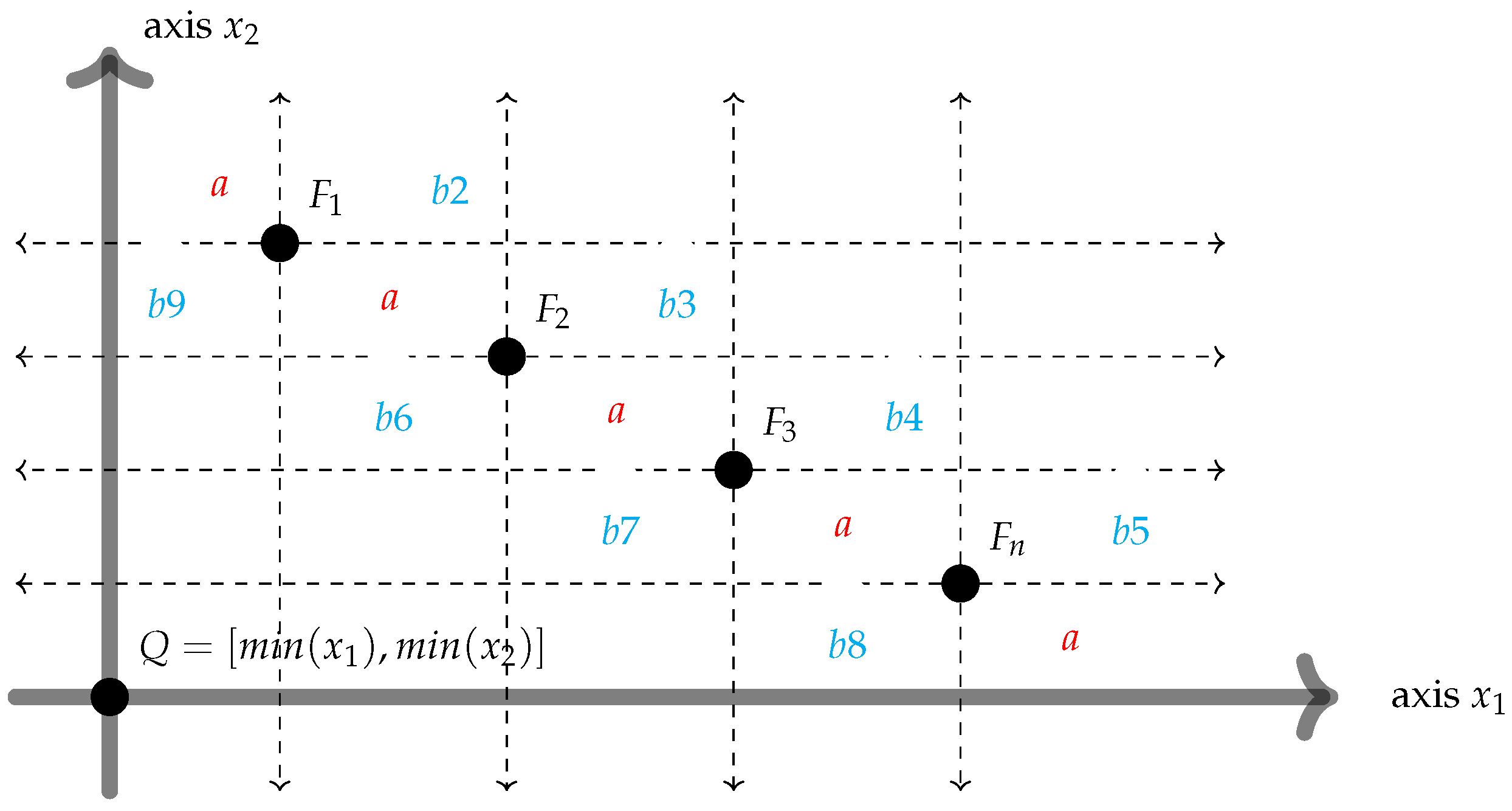
Equation (3) tells us that the bigger dataset $(n+1)$ will contain at least a front or a line of size n and $({(n+1)}^2-n)$ number of points that are in some configuration around them. This is depicted in Figure 7 and Figure 8.

In Figure 7 and Figure 8 the red areas a indicate areas where we cannot fit any more points or we end up with $OR\left[(n+1)L,(n+1)F\right]$, meaning all the $({(n+1)}^2-n)$ points must be somewhere in the blue areas marked with b. Clearly, if we fit all $({(n+1)}^2-n)$ within the same area, we produce at least one $OR\left[(n+1)L,(n+1)F\right]$. Therefore, at best, we can try splitting the points evenly across the n line or front points. As a result we end up with at least as many points as shown in Equation (4).

$${\displaystyle \frac{({(n+1)}^2-n)}{n}}={\displaystyle \frac{n^2+2n+1-n}{n}}=n+1+{\displaystyle \frac{1}{n}}$$

(4)

Therefore we have produce at least one $OR\left[(n+1)L,(n+1)F\right]$ by the pigeonhole principle. This proves Equation (1).    □

3. CDF Manifold Algorithms

To describe the implementation of the CDF manifold algorithm we start by giving the pseudocode for vector comparison in Algorithm 1.

Algorithm 1: Vector comparison for dictionary sort

Require: Input vector $\overrightarrow{A}=[a_1,a_2\dots a_d]$ and input vector $\overrightarrow{B}=[b_1,b_2\dots b_d]$   1: $i=1$   2: while  $i\le d$  do   3:     if  $a_i=b_i$ then   4:         $i=i+1$   5:     else   6:         if  $a_i<b_i$ then   7:             return return statement $\overrightarrow{A}<\overrightarrow{B}$   8:         else   9:             return return statement $\overrightarrow{A}>\overrightarrow{B}$ 10:         end if 11:     end if 12:     $i=i+1$ 13: end while 14: return return statement $\overrightarrow{A}=\overrightarrow{B}$

By using Algorithm 1 to compare vectors we can then apply it to compare instances in a merge-sort procedure [12], which defines a dictionary sort. If the data is sorted in a dictionary, then, if we compare $data(i,:)$ to $data(i+1,:)$ using Algorithm 1, the result would be that $data(i,:)\le data(i+1,:)$. The dictionary sort is given in Algorithm 2.

Algorithm 2: Adapting merge sort using Algorithm 1 to obtain a dictionary

Require: Input data matrix $data$   1: if $data$ has 2 rows then   2:    Compare and sort using Algorithm 1   3:    return   4: end if   5: $mid=rows\left(data\right)/2$ select the middle element of $data$   6: recursive call with $data(1:mid,:)$ to sort first half yielding $hal{f}_1$   7: recursive call with $data(mid:end,:)$ to sort second half yielding $hal{f}_2$   8: $a=1,b=1$   9: for  $i=1$ to  n  do 10:    if  $hal{f}_1(a,:)<hal{f}_2(b,:)$ then 11:        $data(i,:)=hal{f}_1(a,:),a=a+1$ 12:    else 13:        $data(i,:)=hal{f}_2(b,:),b=b+1$ 14:    end if 15:    if $a,b$ last element then 16:      copy the rest and break from loop 17:    end if 18: end for 19: return return $data$

In addition to a dictionary to run searches in the long fronts we need a matrix of indexes, which must be such that $data\left(ind\right(i,k),k)\le data\left(ind\right(i+1,k),k)$. Observe that the matrix $ind$ differs from a dictionary because a row $ind(i,:)$ is no longer a data point as opposed to $data(i,:)$, which is a data point. This index matrix is computed at line 15 in Algorithm 3, where the algorithm itself detects a single long line or a front in a dictionary-sorted dataset.

Algorithm 3: Detecting a single long line or a long front in a dictionary

Require: Input dictionary-sorted data $data(i,:)\le data(i+1,:)\forall i$   1: Initialize a queue for long lines $q_L$   2: Initialize a queue for long fronts $q_F$   3: Initialize A as the last element of $q_L$   4: Initialize B as the last element of $q_F$   5: for  $i=1$ to  n  do   6:     if $data(i,:)$ is AR of $\overrightarrow{A}$ then   7:        add $data(i,:)$ to the long line $q_L$   8:        $\overrightarrow{A}=data(i,:)$ update last element in the long line.   9:     end if 10:     if $data(i,:)$ is not AR and not BL of $\overrightarrow{B}$ then 11:        add $data(i,:)$ to the long front $q_F$ 12:        $\overrightarrow{B}=data(i,:)$ update last element in the long front. 13:     end if 14: end for 15: $in{d}_f=ind\left(q_F\right)$ obtain indexes that sort the front at dimension k. 16: return long line $q_L$, long front $q_F$ and $in{d}_f$.

Algorithm 3 is guaranteed by Theorem 1 to detect either a long line or a long front of length $n^{1/2}$ in the worst case. It is also worth noting that computing $in{d}_f=ind\left(q_F\right)$ takes $O\left(n\right)>O(n^{1/2}ln\left(n^{1/2}\right))$ steps at most. Because we run an exhaustive search over all data points n, the worst possible cost is $n^{1/2}.O\left(n\right)=O\left(n^{3/2}\right)$. Detecting all long fronts and long lines concludes the manifold construction.

Now we describe how we search through the manifold. We start by giving the binary search procedure in a single long line in Algorithm 4.

Algorithm 4: Searching in a single long line

Require: Input search vector $\overrightarrow{X}$ and long line $data(i,:)$ is BL of $data(i+1,:)\forall i$   1: Set $s=1$ as the start of the search interval.   2: Set $t=n$ as the end of the search interval.   3: while  $s\ne t$  do   4:     $mid=(s+t)/2$ compute the middle of the search interval   5:     if  $X(1,1)>data(mid,1)$ then   6:         Set $s=mid$, start of search interval is too small   7:     else   8:         Set $t=mid$, end of search interval is too large   9:     end if 10: end while 11: return  s

Observe that, by computing the $mid$ variable in Algorithm 4, we identify the upper and lower limits of the data within a single long line. Therefore, to find the best, we repeat the procedure across all detected long lines and simply return the tightest bound. Next, consider the binary search procedure in a single long front in Algorithm 5.

Algorithm 5: Searching in a single long front

Require: Input search vector $\overrightarrow{X}$, Require: Long front $data(i,:)$ is not AR and not BL of $data(i+1,:)\forall i$ Require: $in{d}_f$ that sort the dimensions, $data(in{d}_f(i,k),k)\le data(in{d}_f(i+1,k),k)$   1: Set  $k=1$ as the start of the search dimension   2: Set  $g=1$ as the start of the search interval.   3: for  $k=1$ to  d  do   4:     Set $s=g$ as the local start of the search interval.   5:     Set $t=n$ as the local end of the search interval.   6:     while $s\ne t$ do   7:         $mid=(s+t)/2$ compute the middle of the search interval   8:         if $X(1,k)>data(in{d}_f(mid,k),k)$ then   9:            Set $s=mid$, start of search interval is too small 10:         else 11:            Set $t=mid$, end of search interval is too large 12:         end if 13:     end while 14:     Set $g=s$ as the start of the search in the next dimension 15: end for 16: return g

Naturally we need to repeat the search in Algorithm 5 for all long fronts and return the tightest bound. Last but not least the final result is the tightest bound between the long fronts and the long lines. Observe that, in Algorithm 5, we have the requirement to also input the indexes that are computed at step 15 in Algorithm 3.

During a single search, in the worst case there might be as many as $O\left(n^{1/2}\right)$ long fronts or long lines by Theorem 1 and since a search through each long front or long line takes $O(ln(n\left)\right)$ then the total cost is $O(n^{1/2}ln\left(n\right))$.

4. Computing the CDF

Whenever we compute the upper or lower limit of a search point T we always look it up in all long lines and long fronts. If the search point T is positioned at index $s=L_i\left(T\right)$ in a given long line i, then there are exactly s points that contribute to its CDF. In this context the value $s=L_i\left(T\right)$ is exactly the value s that is being returned by the pseudocode in Algorithm 4. Therefore the total CDF contribution by all the long lines is given by Equation (5).

$$CD{F}_{line}\left(T\right)=\sum _i{L}_i\left(T\right)$$

(5)

Similarly, we need to add up the contributions $F_i$ of all fronts to finally obtain the CDF in Equation (6).

$$CDF\left(T\right)=CD{F}_{line}\left(T\right)+\sum _i{F}_i\left(T\right)$$

(6)

Computing $F_i$ in Equation (6) is an exhaustive search in the long front i. However, we can gain some speed by observing that the first binary lookup in the first search dimension in a long front will point out how many points can contribute to the CDF. In other words, in a long front, if the initial binary lookup places the point T at index b, then there are no more than b points that can contribute to $F_i$. However some of the first b points might not be BL of T and will not contribute to the CDF, and in these cases we need to check them one by one. In this context the value b equals g in Algorithm 5 at step 14 only when $k=1$. Better speedup of $F_i$ estimation is left as future work.

5. Numerical Comparison

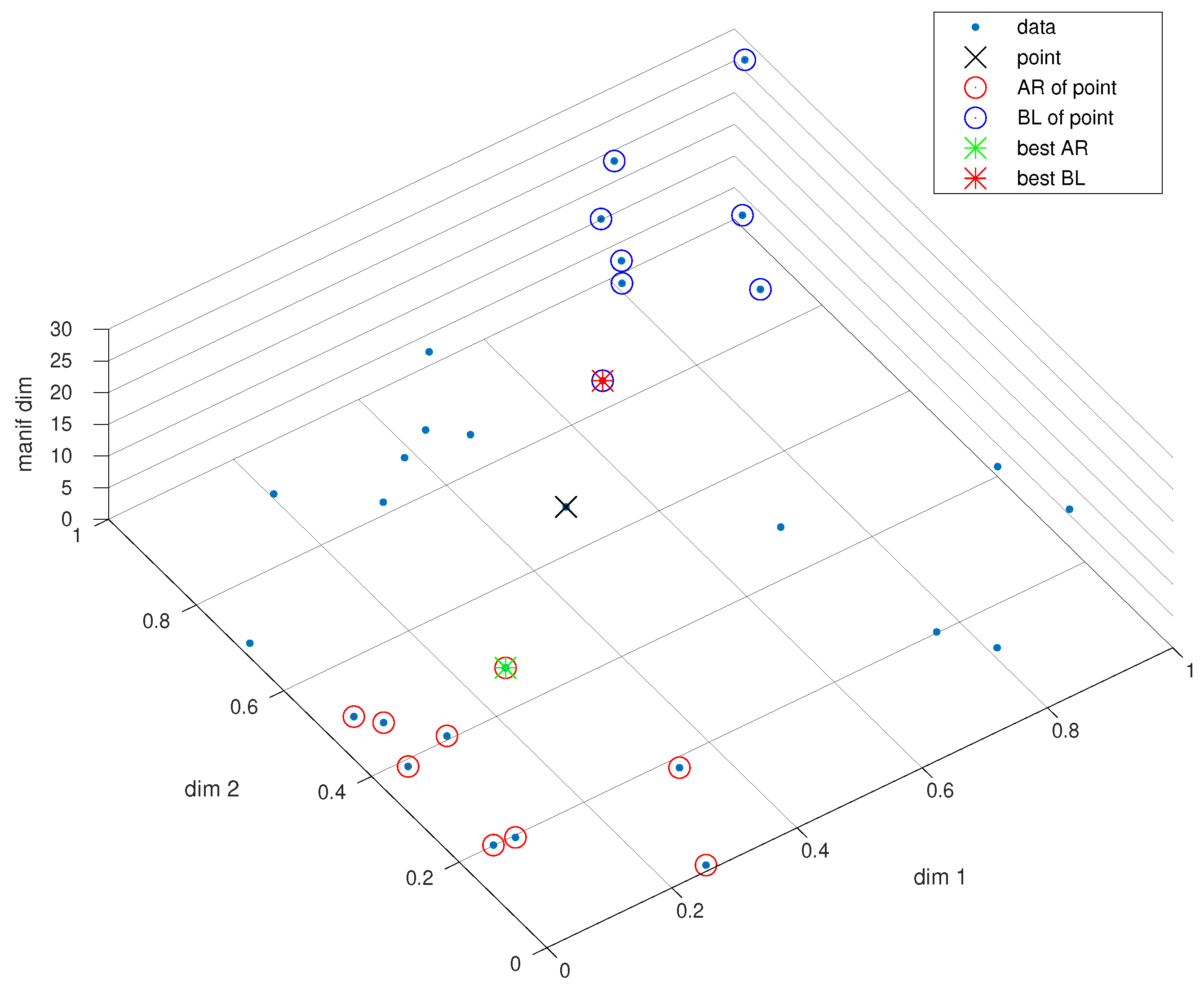
Figure 9 shows an example where the AR and BL were computed for a single point in 3D since the manifold only has meaning where we have at least two input and one output dimensions.

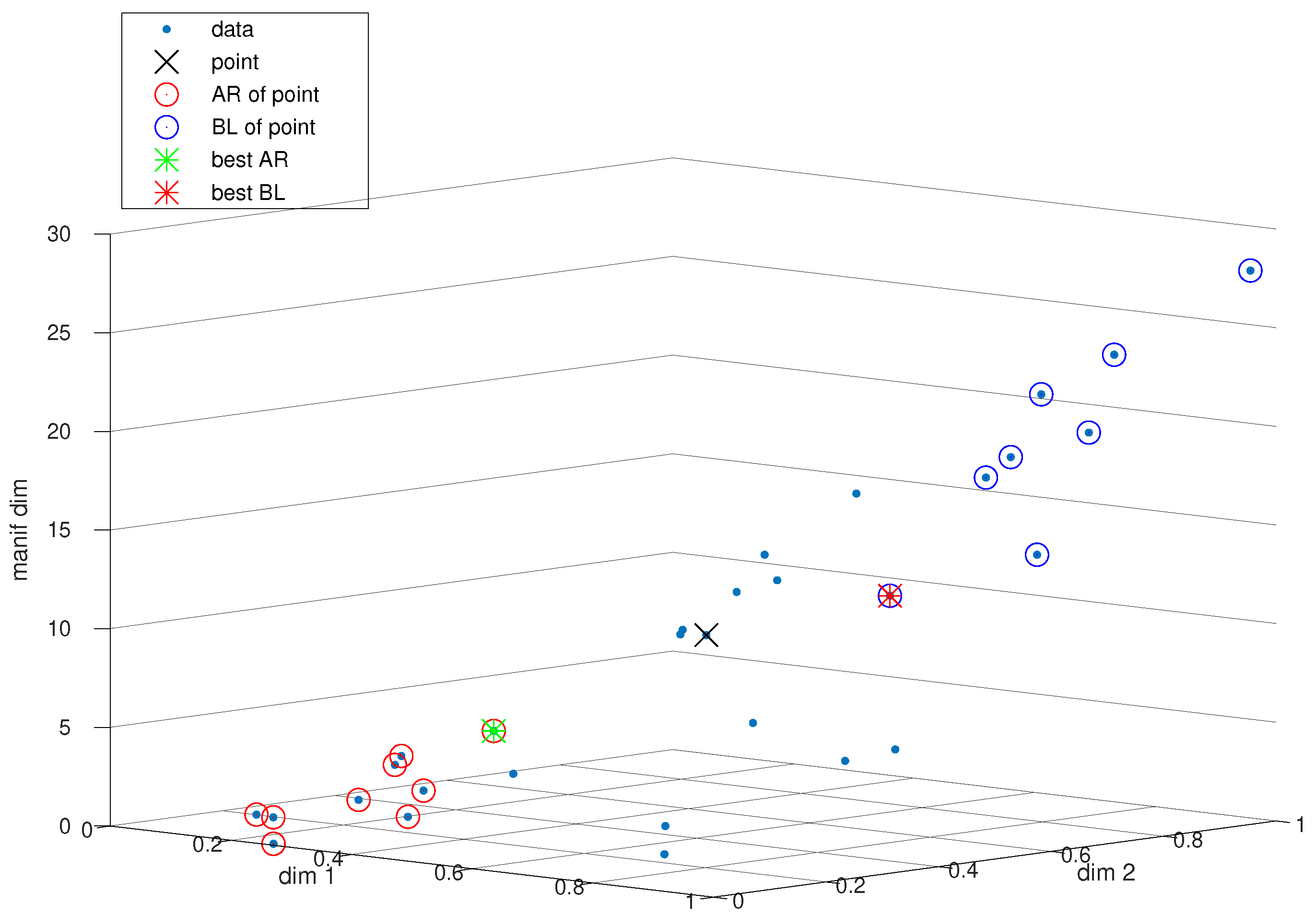
In Figure 9 observe that the AR and BL set might be a huge part of the whole set, meaning computing the optimal limits is difficult. Figure 10 shows a side view of the same example as Figure 9. In Figure 10 observe that the limits might not be very tight, but the result would still be reasonable due to the manifold property.

For the remaining evaluations in this section consider a common telco problem where the base station has gathered three KPIs, namely the UE activity, mean CQI and mean UE throughput, on an hourly basis. For a given UE activity and CQI we would like to compute the mean UE throughput. Observe that increasing the activity separately from the CQI will decrease the throughput. Similarly, increasing the CQI separately from the activity will increase the throughput. Increasing the CQI and decreasing the activity will increase the throughput. Therefore let the first dimension be $x_1=CQI$, while the second dimension is the negative of the activity $x_2=(-1)\ast activity$. The target variable $y=throughput$ is the mean throughput. Therefore $x_1,x_2,y$ have the CDF manifold property.

Next, the input data $x_1$ and $x_2$ is sampled from a standard normal distribution using $rand(\ast )$ in Octave. The true mapping between the data dimensions $x_1$ and $x_2$ is assumed a sum of sigmoid functions $\sigma [\ast ]$ or more specifically $y=\sigma \left[10(x_1+1)\right]+\sigma \left[15(x_1+2)\right]+\sigma \left[5(x_1-1)\right]+\sigma \left[2(x_1+1)\right]+\sigma \left[1(x_1+3)\right]+\sigma \left[3(x_1-3)\right]+\sigma \left[4(x_1-2)\right]+\sigma \left[(x_2-1)\right]+\sigma \left[30(x_2-1)\right]+\sigma \left[30(x_2-2)\right]$. Note that, because a sum of strictly increasing functions is strictly increasing, this mapping has the CDF manifold property. This elaborate mapping from x to y was chosen to make sure we observe a lot of errors made by the manifold and comparison model.

Consider benchmarking against other non-parametric methods. Practically all known non-parametric methods do not have built-in mechanisms to respect the strictly increasing property. K-nearest neighbor will return the closest neighbor even if it is not in line with the increasing property. Gaussian processes are not sensible for benchmarking as the KPIs in question rarely have a normal distribution. Additionally kernel methods will fail to generalize well because they do not have mechanisms to respect the strictly increasing property.

A decision tree (DT) is a good benchmarking candidate, but it lacks the functionality to look for upper and lower bounds and compute the CDF or outperform NN in general. Furthermore, in practice, when engineers deploy new sites, they are very much interested in guaranteed performance, and they would often use an NN over DT just to reduce the prediction error even if the model is no longer explanatory.

With the proposed manifold we try to establish guaranteed performance limits while also adhering to the most common telco practices. Since NNs are also considered cutting-edge manifold methods that are often the first choice for any benchmarking, we select an NN for evaluation. Nevertheless comparing the manifold against a DT is a good direction for future work.

It is worth noting at this point that a new algorithm does not need to outperform all known methods on all datasets in order for the algorithm to be novel or find a niche use. The goal of the comparison is not to find the best-in-slot components but showcase a reasonable alternative.

Next, the NN below has only one layer because the test function we use is a sum of sigmoids, which is also expressed as an NN with one layer. The only difference is that in practice we could never know exactly how many neurons to use, especially in higher dimensions. Hence let the NN have a single layer with 16 neurons. In practice we would never know the true number of NN layers that model the data, and therefore setting it to the exact right value of one gives the NN a slight advantage over the manifold.

The NN is trained for 400 iterations using Octave’s $fminunc(\ast )$ function applied to the forward–backward propagation algorithm. To compare the NN to the manifold we compute the Root Mean Square Error (RMSE) and a separate swap metric.

The swap metric counts the number of times the prediction does not adhere to the strictly increasing property. Meaning, for a data prediction point t, we find the indexes of all training points $I_{ar}[x\in AR\left(t\right)]$ that are $AR$ of t and then count how many of them had y values that were not AR of the prediction $y_p$ or more explicitly $y\left(I_{ar}\right)\notin AR\left(y_p\right)$.

We start the simulation with a sample of 40 data points, then compute the error measures and then add 40 new sampled data points to the original set. We repeat sample and addition until we get to a sum total of 800 points. The reason behind this is to simulate how KPIs get added over time as the base station obtains more and more real-life measurements.

Additionally, the data is split into training and validation sets using a 50/50 ratio. We train the models on their respective training sets and evaluate the RMSE and swap metrics on the validation sets. The exact numerical results are given in

Table 1. The exact dataset used to produce Figure 11.

Data Size	Swap NN	RMSE NN	Swap MANIF	RMSE CDF
40	3	0.3484	1	0.4087
80	1	0.2781	6	0.2557
120	15	0.4558	1	0.2827
160	12	0.2559	6	0.2669
200	5	0.2846	10	0.1745
240	44	0.2513	8	0.2750
280	4	0.2443	24	0.1654
320	149	0.3214	18	0.1792
360	25	0.2932	20	0.2135
400	55	0.2789	51	0.2158
440	86	0.2465	65	0.2217
480	42	0.2887	67	0.1635
520	199	0.2757	49	0.1649
560	81	0.3073	49	0.1760
600	0	0.4709	57	0.1854
640	423	0.2603	32	0.2263
680	158	0.2963	73	0.1728
720	119	0.3038	58	0.1627
760	542	0.2757	98	0.2042
800	63	0.2900	57	0.1729

.

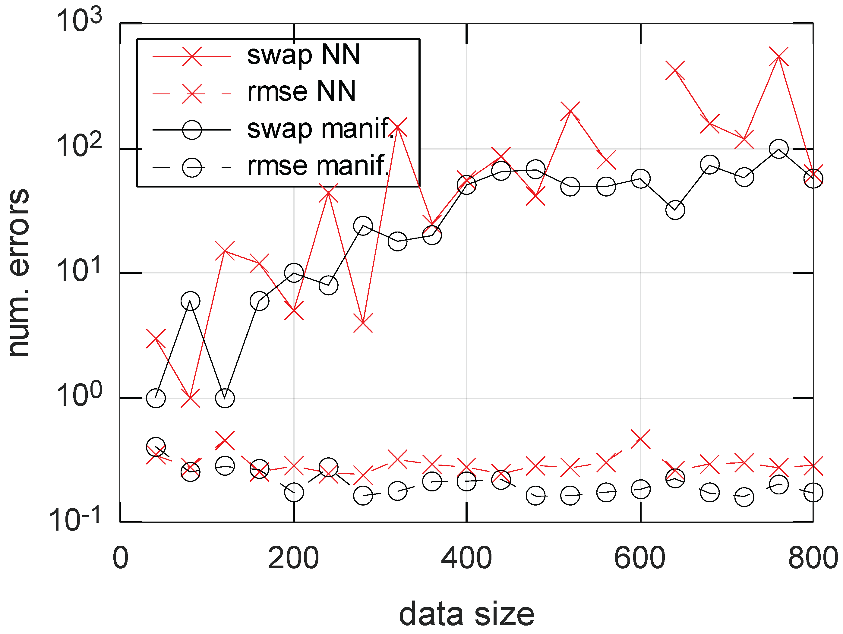
The data in Table 1 is used to produce Figure 11, where the Y-axis is on a logarithmic scale because the measures have different scales and the X-axis is the number of input data for each estimation. The columns of Table 1 have the same names as the corresponding objects in Figure 11.

In Figure 11 we see that the RMSE gradually decreases for both models as we get more and more data. The RMSE of the NN flattens after we reach around 200 samples, while the manifold experiences improved performance with each new data point.

Both the NN and the manifold can experience swaps in the strictly increasing data property, but the manifold swaps are more reliable and in many cases at least 1 order of magnitude better than the NN.

Interestingly, for data size 600, the NN had zero swaps, which does not guarantee it will not swap an unseen input at all because it is difficult to ensure continuous NN mapping if strictly increasing everywhere. On the other side, with a large enough dataset, the manifold will make fewer and fewer swaps while the RMSE will keep decreasing.

Therefore, as future work, it would be interesting to see if there is an ensemble model that can take advantage of both the NN and the manifold.

Computational Complexity Comparison

To start the complexity comparison observe that the computational cost of a single NN training, even with Strassen’s multiplication, is $O\left(n^{2.7}\right)$, while the CDF manifold costs in the worst case $O\left(n^{3/2}\right)$, meaning the manifold runs more than $O\left(n\right)$ times faster. In fact, depending on the data, the manifold might cost only $O(n.ln[n\left]\right)$, which is an improvement of at least $O\left(n^2\right)$. Furthermore the manifold is an explanatory model where we know exactly which two data points produced the prediction, while the NN acts as a black box that does not have a clear reason for any given prediction.

Predicting for a single data vector using the NN costs $O\left(w^{2.7}\right)$, where w denotes the number of parameters or neurons the network has, which would then be used for matrix multiplication, which reverts to Strassen’s algorithm again. On the other hand predicting for a single input vector with the manifold takes $O\left(log\right[n\left]\right)$ in the best case, when the data is ordered in either a few long lines or a few long fronts. In the worst case we need to search as many as $O\left(n^{1/2}\right)$ lines and fronts by Theorem 1 and the cost becomes $O\left(n^{1/2}ln\left(n\right)\right)$.

Referring to Equation (6), computing the CDF for a single data input takes in the best case $O\left(log\right[n\left]\right)$ when the data has few long fronts. Alternatively, if the data has mostly long fronts or one giant long front, then we need to conduct a linear scan at a cost of $O\left(n\right)$. For clarity, in

Table 2. Comparing the computational complexity.

Name	Worst Case	Best Case
train NN	$O\left(n^{2.7}\right)$	$O\left(n^{2.7}\right)$
train manifold	$O\left(n^{3/2}\right)$	$O(n.log[n\left]\right)$
predict NN	$O\left(w^{2.7}\right)$	$O\left(w^{2.7}\right)$
predict manifold	$O\left(n^{1/2}ln\left(n\right)\right)$	$O\left(log\right[n\left]\right)$
compute single CDF	$O\left(n\right)$	$O\left(log\right[n\left]\right)$

, we summarize the computational complexity.

6. Conclusions

In this paper we introduced the CDF manifold that on average can be constructed in $O(n.ln(n\left)\right)$ steps, with the worst case costing $O\left(n^{3/2}\right)$. Searching with a single new instance is expected to cost $O\left(ln\right(n\left)\right)$ steps and $O\left(n^{1/2}ln\left(n\right)\right)$ in the worst case.

The manifold also relies on the dictionary algorithms of the package in [11]. The same manifold can also be used to compute the CDF of either a data point or a new data point, as described in Section 4. Both the construction and the search algorithms can be parallelized.

The algorithm is expected to perform best with telecom data where the KPIs have physical system meaning that keeps them bound within certain limits, which increases the likelihood of containing singular long fronts and long lines. In addition, telco data is highly likely to be strictly increasing, which satisfies the prerequisites of the algorithm.

We also did a simulation study to compare the performance of an NN and the CDF manifold. The results showed that, for large datasets, the computational complexity, the achievable accuracy and the explanatory characteristics of the search algorithms point in favor of the manifold.

Future work consists of considering various reference-point approaches because we saw how the inversion-point heuristic can help to speed up construction. It would also be interesting to search for even faster ways to compute the CDF of a point given the manifold. Another future work project would be considering hybrid models between the CDF manifold and a neural network, for example, or comparing the manifold to a decision tree.