Classifying and Predicting Household Energy Consumption Using Data Analytics and Machine Learning

Abstract

Growing pressure on electricity grids and the increasing availability of smart meter data have intensified the need for accurate, interpretable, and scalable methods to analyze and forecast household electricity consumption. In this context, this study presents a general, data-agnostic methodology for predicting and classifying household energy consumption. The proposed workflow unifies data preparation, feature engineering, and machine learning techniques (including clustering, classification, regression, and time series forecasting) within a single interpretable pipeline that supports actionable insights. Rather than proposing new prediction algorithms, this work contributes a fully reproducible, end-to-end methodological pipeline that enables the controlled evaluation of the impact of contextual variables, customer segmentation, and cold-start conditions on household energy forecasting. A distinctive aspect of the pipeline is the explicit use of household- and dwelling-level contextual variables to derive customer typologies via clustering and to enrich forecasting models. The models are evaluated for predictive accuracy, reliability under varying conditions, and suitability for operational use. The results show that incorporating contextual variables and clustering significantly improves forecasting accuracy, particularly in cold-start scenarios where no historical consumption data are available. Although numerous public datasets of residential electricity consumption exist, they rarely provide, in an openly accessible form, both detailed load histories and rich contextual attributes, while many are subject to privacy or licensing restrictions. To ensure full reproducibility and to enable controlled experiments where contextual variables can be switched on and off, the experiments are conducted on a synthetically generated dataset that reproduces realistic behavior and seasonal usage patterns. However, the proposed methodology is independent of the specific data source and can be directly applied to any real or synthetic dataset with similar structure. The approach enables applications such as short- and long-term demand forecasting, estimation of household energy costs, and forecasting demand for new customers. These findings demonstrate that the proposed pipeline provides a transparent and effective framework for end-to-end analysis of household electricity consumption.

1. Introduction

Growing concerns on electricity grids, rising energy costs, and the environmental consequences of over-consumption have increased the urgency for efficient household energy use and management. Advances in smart meters and compact sensors now allow detailed monitoring of residential consumption, enabling data-driven approaches for analysis and optimization. Recent studies have used such data to classify appliance-level events, identify consumption patterns, and forecast short-term demand with models such as LSTM and ARIMA [1,2]. Building on this work, the present study introduces a three-stage methodological pipeline for the analysis, segmentation, and forecasting of household electricity consumption. Although our broader motivation relates to the use of low-cost sensor devices attached to existing meters, the proposed methodology is fully data-agnostic and can be applied to any dataset with similar structure. A central aspect of the approach is the explicit use of contextual variables (household composition, dwelling characteristics, heating/cooling systems, teleworking status) to generate customer typologies via clustering and to guide the construction of specialised forecasting models. These contextual attributes are also essential for mitigating the cold-start problem for new customers by enabling cluster-based reconstruction of lagged features. Despite the existence of numerous public datasets of residential electricity consumption, most openly accessible versions provide only load measurements without the associated household or dwelling characteristics needed for segmentation or cold-start forecasting. Datasets that do include rich contextual information are typically subject to privacy or licensing restrictions. Since no real sensor data are available, and in order to support reproducibility, all data are synthetically generated and publicly released to simulate the expected behavior of such devices. The simulated measurements capture electricity usage at fine temporal granularity and are designed to be scalable for large-scale deployment. Model performance is evaluated in terms of accuracy, robustness, and operational relevance. Interpretability is emphasized so that outputs yield actionable insights, such as clustering customers based on consumption patterns, forecasting demand for existing customers, and predicting consumption for new customers, with attention to identifying the most influential features and characteristics. Additionally, we quantify the loss in forecasting accuracy when contextual variables are removed and clustering becomes impossible, demonstrating substantial performance degradation in both existing and new-customer scenarios. This confirms the methodological value of integrating contextual information within the proposed pipeline.

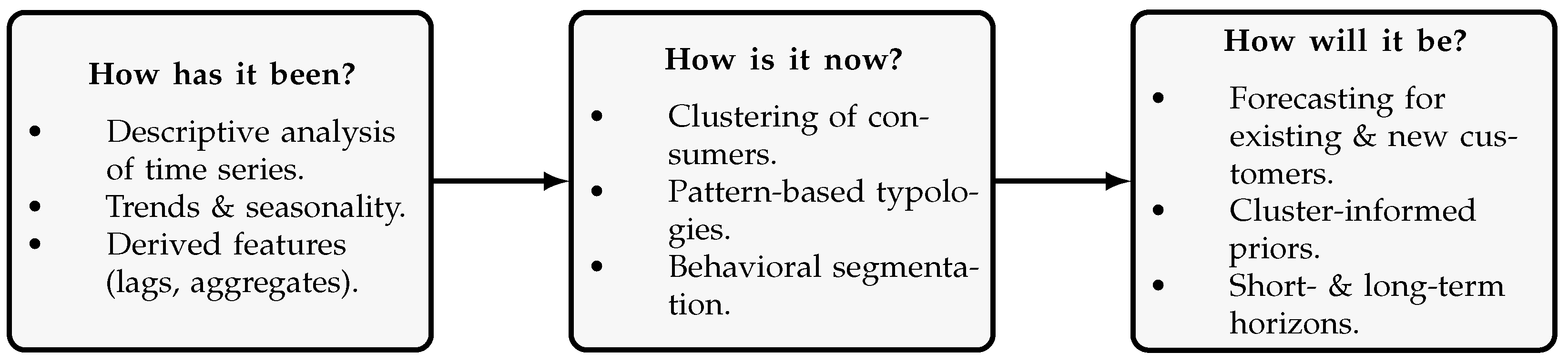
The main contribution of this work is a unified methodological pipeline that integrates descriptive, unsupervised, and predictive analyses. This approach enables a comprehensive understanding of household electricity consumption while ensuring interpretability for practical applications. The proposed framework addresses three fundamental questions about household electricity consumption:

1.

“How has it been?” The first stage performs a descriptive analysis of historical time series, extracting trends, seasonalities, and derived features that characterize consumption patterns at different temporal resolutions.

2.

“How is it now?” The second stage applies clustering methods to group consumers according to their historical consumption patterns. This allows the identification of customer typologies and recurrent behaviors that can inform personalized energy management strategies.

3.

“How will it be?” The final stage develops forecasting models to predict future demand, both for existing customers and for new customers with no historical consumption data. These predictions are refined using the cluster assignments obtained in the previous stage, which serve as a structural prior for characterizing new customers.

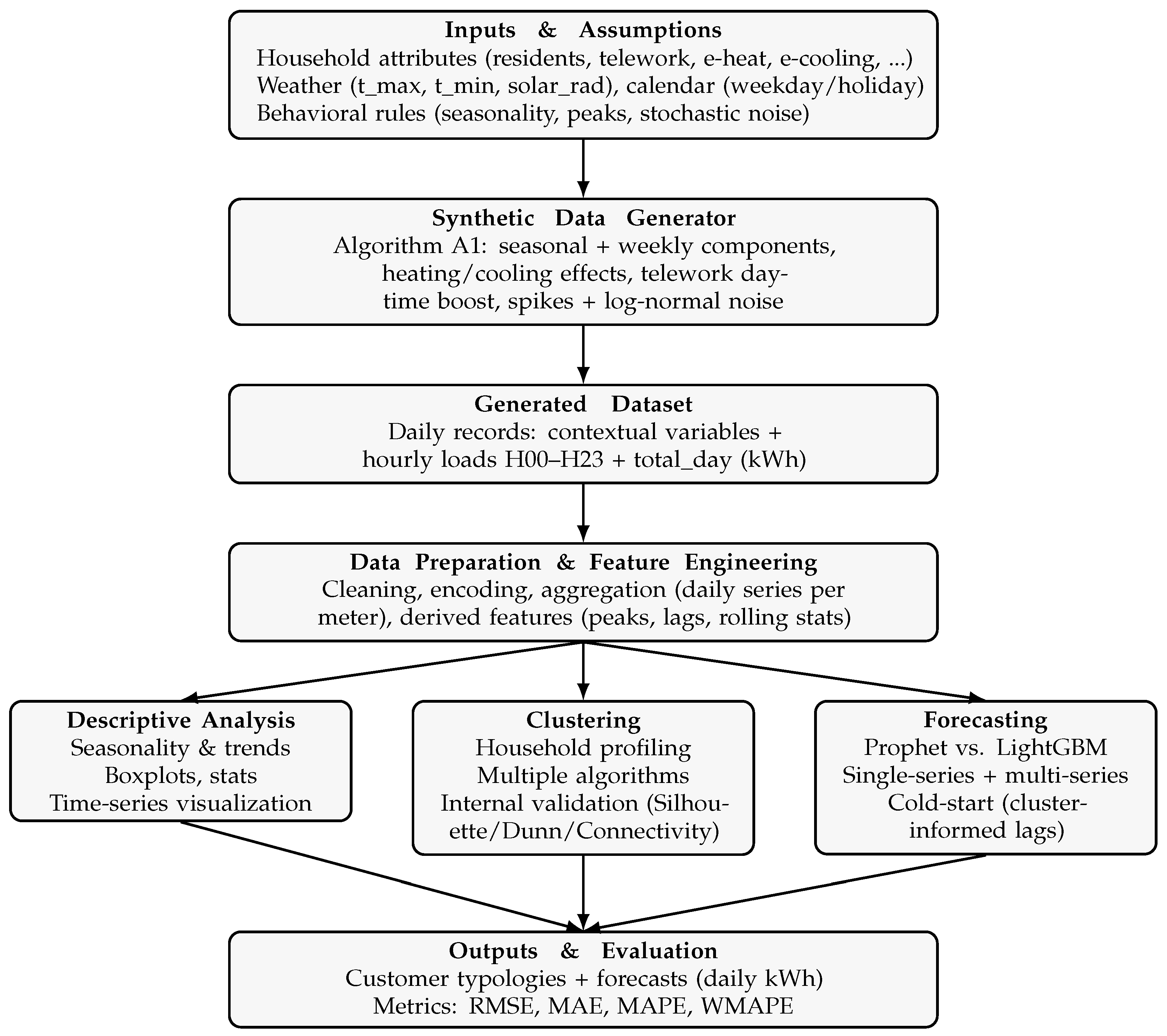
Together, these stages form a methodological pipeline that provides a coherent view of consumption behavior across past, present, and future dimensions. Figure 1 and Figure 2 provide a conceptual and operational overview of the proposed pipeline.

Although the individual techniques employed in this work—such as clustering, tree-based ensemble models, and time series forecasting—are well established, the novelty of this study lies in their integration into a single, fully reproducible, end-to-end methodological pipeline. Unlike prior studies that focus on isolated tasks (e.g., forecasting or segmentation alone), the proposed framework explicitly links household- and dwelling-level contextual variables with descriptive analysis, unsupervised segmentation, and forecasting within a coherent workflow. In particular, the pipeline is designed to address the cold-start problem for new customers by leveraging cluster-informed reconstruction of lagged features, enabling forecasting even in the absence of individual historical data.

The rest of the paper is structured as follows. Section 2 reviews the prior research on data analytics and machine learning for residential energy use. Section 3 outlines the synthetic data structure and generation process. Section 4 presents a descriptive analysis of the generated data. Section 5 presents an exploration of time series data, including examples, and different types of consumption patterns derived from the characterization of the series. Section 6 explores different clustering approaches for segmenting customers according to their consumption behavior. Section 7 presents forecasting models for electricity consumption, addressing both short-term and long-term horizons, for existing as well as new customers. Section 8 summarizes contributions and suggests directions for future work.

2. Related Work

Several studies focus on forecasting household electricity consumption using deep learning and hybrid approaches. Kiprijanovska et al. [3] introduced HousEEC, a deep residual neural network that integrates historical load, contextual, and time-series data for day-ahead forecasting, outperforming several benchmarks on the Pecan Street dataset and handling cold-start and missing data. Similarly, Yang et al. [4] proposes Co-LSTM, a combined deep learning model that captures both long- and short-term consumption patterns for individual households. Using clustering and feature reduction, Co-LSTM achieved around $5\%$ better accuracy than traditional LSTM on 71 Pecan Street households. Pai et al. [5] enhanced multivariate LSTM models by integrating weather data, achieving higher household-level accuracy. Priyadarshini et al. [6] developed an ensemble model merging decision trees, random forest, and XGBoost for smart home energy forecasting with near-perfect $R^2$ scores on datasets with one-minute readings, outperforming baseline models. These approaches demonstrate the strong predictive power of deep learning and tree-based ensembles for household energy consumption forecasting, but they typically focus on a single task (prediction) and pay limited attention to integrating forecasting with exploratory and segmentation analyses.

Other works explicitly combine feature engineering and model selection with hybrid or automated frameworks. Iram et al. [7] designed a decision algorithm using weather data with feature selection via PCA and Lasso regression. Support vector regression showed the best results, and an automated matrix selects models based on multiple criteria. Kim et al. [8] combined time-series clustering with forecasting on smart meter data to identify household demand patterns, showing that clustering-based segmentation improves prediction accuracy. Haq et al. [9] proposed a hybrid approach that combines k-medoids clustering, SVMs, and neural networks to forecast appliance-level consumption and peak demand, reaching $99.2\%$ accuracy on smart meter data. Alkhulaifi et al. [10] introduced AutoEnergy, an AutoML-based feature engineering framework that automates predictor selection and significantly improves forecast accuracy. Rauf and Adekoya [11] used a hybrid ARIMA-SVM model to forecast electricity use in Northern Ghana, highlighting family size as a key factor. Overall, hybrid and AutoML-based methods improve predictive performance and reduce manual tuning, but they usually treat clustering, feature engineering, and forecasting as unconnected components rather than as parts of an interpretable, end-to-end workflow that also can predict consumption for new customers without historical data.

Machine learning models applied to specific energy types or regions also appear. Raviprabhakaran et al. [12] used XGBoost to forecast household active power, identified water heaters and air conditioners as key drivers, and suggested variables such as holidays to further improve accuracy. Dinmohammadi et al. [13] used PSO-optimized random forest and ensemble stacking to predict residential heating energy consumption with $95.4\%$ accuracy. Wu et al. [14] studied household energy disparities in China with machine learning and survey data from 3637 households, identifying consumption types and regional differences. Henriques et al. [15] compared clustering methods to classify residential energy patterns in Brazil, finding k-means the most accurate. They balance consumer and provider perspectives to inform policy and resource management, noting the need for more granular regional data. These studies tend to focus on forecasting or consumption pattern recognition, rather than an integrated loop that goes from descriptive analysis to segmentation and then to forecasting. In particular, Dinmohammadi et al. [13] and Wu et al. [14] highlight the importance of context variables such as weather data or socio-demographic factors.

Several studies focus on the use of machine learning for understanding and managing household energy consumption with a policy or demand response angle. Cui et al. [16] developed separate models for U.S. apartments and single-family houses using tree-based algorithms. LightGBM and CatBoost performed best, with $R^2$ around $0.69$. SHAP analysis identified key household features, supporting targeted energy-saving measures. Amayri et al. [17] introduced a method to identify flexible appliance use from low-resolution smart meter data using random forest and clustering, enhanced by interactive learning with user feedback. This helps design demand response programs and can adapt to emerging devices. Burnett and Kiesling [18] compared multiple machine learning models for U.S. household energy demand, finding random forest best. They discussed applications including demand response targeting and electric vehicle-to-grid integration. Alzoubi [19] reviewed machine learning methods in smart home energy management and load forecasting, noting data fusion techniques that improve accuracy up to $92\%$ and suggesting future research for energy efficiency. Zhou and Yang [20] proposed a framework combining energy, social, and information sciences using big data analytics to understand household energy behavior and support targeted interventions. These contributions underline the value of interpretability, but they typically do not provide a generic and reusable methodology that addresses multiple aspects of the analysis, allowing for descriptive profiling, clustering and forecasting.

Regarding model benchmarking and method comparison, Seyedzadeh et al. [21] reviewed ML methods for building energy estimation, emphasizing trade-offs between data volume, complexity, and scalability. Chou and Tran [22] compared multiple forecasting models on smart grid data, showing that hybrid SARIMA–SVR combinations outperform single and ensemble models. They recommend including weather variables in future studies. Similarly, Veit et al. [23] found that simple persistence models can rival more complex methods, underscoring the need for consistent benchmarking and the integration of richer features such as occupancy information and improved data handling. These works show that simple models remain competitive against more complex ones, highlighting the use of both autoregressive and exogenous features, but they mainly focus on model performance rather than standardizing a general pipeline that covers an end-to-end analysis of household energy consumption.

Studies combining socioeconomic and weather data for energy use prediction include Chowdhury et al. [24], who used random forest to predict U.S. household energy consumption, outperforming logistic regression and SVM. This model can support demand management and conservation. Tang et al. [25] applied K-medoids clustering to smart meter and socioeconomic data, identifying twelve load patterns and developing a deep learning model that reduced errors by $46\%$. Their results can aid demand response targeting. These works illustrate the benefits of integrating contextual and behavioral variables together with consumption-pattern segmentation, but they offer limited interpretability and provide little discussion on how to extract actionable insights from the resulting models.

Finally, some studies emphasize scalable and efficient forecasting methods. Botman et al. [26] proposed a lightweight approach for monthly household electricity prediction up to one year ahead using limited historical data and no weather inputs, achieving top-ranking performance in benchmarking tasks. Gao et al. [27] combined online search data with a Jaya-optimized extreme learning machine for monthly residential electricity forecasts in China, improving accuracy by over $10\%$ and reducing errors significantly compared to benchmarks. They recommend expanding data sources in future research. Together, these approaches show that accurate long-term forecasts can be achieved even with limited data, but they focus exclusively on monthly predictions and do not link forecasting with descriptive analysis or clustering, in contrast to the integrated multi-stage pipeline pursued in the present work.

The present work addresses these gaps by proposing a methodological pipeline that begins with descriptive time series analysis, continues with clustering-based segmentation, and culminates in forecasting models for both existing and new customers. The pipeline relies on a synthetically generated dataset that reproduces realistic household consumption patterns under explicit assumptions on weather, socio-demographic characteristics, and behavioral factors. This design enables transparent and reproducible experimentation with different modeling choices, supports both short- and long-term forecasting, and allows cluster-informed predictions for new customers, thereby complementing previous research that has typically focused on individual components of the analysis rather than on an integrated, end-to-end framework.

Public Datasets for Household Electricity Consumption

A large number of public datasets provide detailed measurements of residential electricity use, mostly with a focus on load profiles and appliance-level disaggregation. For example, Alkhulaifi et al. [10] use the Appliances dataset available on Kaggle [28], which contains electricity consumption data for multiple household elements. Similarly, Iram et al. [7] use the Weather VS Energy dataset (also available on Kaggle [29]), which combines electricity consumption with contextual features such as weather and environmental characteristics. However, it lacks multiple time series (covering only a single household). These datasets are widely used for tasks such as load forecasting or pattern recognition, but the publicly available contextual information on building characteristics and occupant socio-demographics is either limited or only partially documented.

Beyond pure load profiling, a smaller set of datasets explicitly link large smart meter readings of multiple households with socio-demographic or building-related information, such as the Pecan Street dataset used by Kiprijanovska et al. [3], Yang et al. [4] and Tang et al. [25]. However, the Pecan Street dataset as mirrored on Kaggle [30], which provides highly granular electricity data for several hundred US households, does not include contextual information such as dwelling characteristics or occupant socio-demographics. This dataset is primarily used for load forecasting, appliance-level disaggregation, and pattern recognition tasks, but the lack of available contextual variables limits the analysis of how household attributes influence consumption patterns. Full access to contextual data, including socio-demographic and building-related attributes, is available through Pecan Street’s Dataport, which is restricted and requires a formal application.

Overall, the existing studies demonstrate that contextual variables can play an important role in explaining residential electricity use. However, they also present several limitations from the perspective of methodological benchmarking. First, publicly available datasets rarely combine high-frequency consumption, detailed household and building attributes, and weather variables in a single, openly accessible resource. Second, many datasets with rich contextual information (such as Pecan Street) are subject to licensing, privacy, or access restrictions that prevent unrestricted redistribution and make full reproducibility difficult. Third, available datasets are often tied to specific regions or regulatory contexts, which complicates controlled experiments where model assumptions and external conditions can be systematically varied.

In this work, we therefore take a complementary approach: instead of relying on one particular real-world dataset, we design a synthetic data generator that explicitly encodes household composition, income, dwelling size, heating and cooling equipment, teleworking, and weather effects. This allows us to create a fully documented, reproducible benchmark where contextual variables can be turned on and off in a controlled way, and their marginal contribution to forecasting accuracy can be quantified. The synthetic dataset does not aim to replicate any specific country or utility, but rather to reproduce realistic patterns and heterogeneity observed in empirical studies while avoiding privacy and licensing constraints.

3. Generating Synthetic Data

The dataset was organized into three main categories of variables, each representing a different aspect of household energy consumption. First, static variables define household characteristics that remain constant for each customer-meter pair, such as meter location, physical attributes of the dwelling, and socio-demographic factors. Second, dynamic daily variables capture conditions that vary day-to-day, including temporal descriptors (e.g., date, weekday, holidays), meteorological parameters (e.g., temperature, solar radiation), and hourly electricity consumption measurements. Third, derived variables were computed from the hourly consumption data to provide deeper insights into usage patterns, such as peak demand periods and event-based consumption characteristics.

Table 1. Summary of variables included in the simulation model.

Variable	Description	Type	Unit
Static variables (household & meter characteristics)
id_met	Meter ID	Categorical	–
id_cust	Customer ID	Integer	–
zip	Postal ZIP code	Categorical	–
loc_met	Meter location (indoor/outdoor)	Categorical	–
area	Heated/cooled floor area	Continuous	m2
residents	Total number of residents	Integer	persons
children	Residents under 18	Integer	persons
adults	Residents aged 18–70	Integer	persons
seniors	Residents over 70	Integer	persons
income	Monthly household income	Continuous	euros
h-work	Telework activity from home	Categorical	yes/no
e-heat	Electric heating system	Categorical	yes/no
e-cooling	Air conditioning presence	Categorical	yes/no
Dynamic daily variables (temporal, meteorological, consumption)
date	Date of record	Date	yyyy-mm-dd
day_week	Day of the week	Categorical	–
month	Month	Integer	1–12
holiday	Holiday/weekend indicator	Categorical	yes/no
t_max	Maximum daily temperature	Continuous	°C
t_min	Minimum daily temperature	Continuous	°C
solar_rad	Daily solar radiation	Continuous	MJ/m2
H00–H23	Hourly electricity consumption	Continuous	kWh
Derived variables (from hourly consumption)
total_day	Total daily electricity consumption	Continuous	kWh

summarizes the variables used, along with their types and units.

This database design provides a foundation for analyzing household energy use, training predictive models, and supporting demand management strategies. To generate realistic consumption profiles, the data generator combines seasonal patterns, behavioural attributes, multiplicative stochastic components, and non-Gaussian distributions (e.g., log-normal) that naturally lead to heterogeneous consumption profiles. The following assumptions and constraints were applied:

• Seasonal variation: electric-heated homes reduce usage in summer, while air-conditioned households show higher cooling demand. In our model, higher consumption during summer and winter holidays is implicitly captured through the annual seasonality component, while a weekly pattern introduces recurring intra-week variations.
• Household composition: the number and age of residents shape baseline and hourly usage; families with children show evening peaks (e.g., appliance use, cooking), whereas seniors use more energy during daytime.
• Teleworking: as reflected in Stikvoort et al. [31], remote work increases daytime consumption and flattens morning peaks.
• Heating and cooling systems: system type and presence determine seasonal and daily demand profiles.

Overall, the combination of behavioural rules, seasonal modulation, truncated and log-normal components, and multiplicative noise ensures that the resulting dataset captures realistic variability and skewed consumption patterns, rather than relying on any single parametric distribution.

As described in Algorithm A1, the dataset is generated through a structured, multi-step process that aims to produce realistic daily and hourly energy consumption data that reflect household and environmental factors. The procedure starts by defining a set of geographic zones (zip codes) with characteristic weather patterns. Each zone (zip code) is assigned an average income per resident drawn from a normal distribution. For each day in the target date range, maximum and minimum temperatures follow a seasonal sinusoidal pattern with added random noise, while solar radiation is drawn from a normal distribution truncated at zero to ensure physically plausible positive values. Individual customers are then simulated with demographic and household attributes. Each customer is randomly assigned a zip code, and a household composition (number of children, adults, and seniors), from which household size is derived. Income is drawn from a normal distribution with a lower bound to avoid unrealistic values, and home area is sampled from a log-normal distribution to capture the typical right-skewed distribution of dwelling sizes, introducing structural heterogeneity in the data. Additional binary features, including teleworking, electric heating, and electric cooling, are sampled probabilistically to introduce behavioral heterogeneity.

Meters are then assigned to households, with each customer having at least one ‘house’ meter, and $20\%$ of customers randomly receiving an additional ‘garden’ meter to add variability. Daily consumption is generated for each meter over the full date range. The base consumption is set according to meter type and modulated by multiple factors. Seasonal and weekly variations are modeled to preserve autocorrelation, while heating and cooling effects are modeled to follow household features and seasonal peaks. Random daily noise represents natural variability. Hourly consumption is constructed by combining morning and evening peaks, temperature-dependent effects that interact with the hour of day, telework boosts on weekdays, occasional random spikes representing irregular high-usage events, and multiplicative log-normal noise to increase realism. Hourly consumption is clipped to prevent unreasonably low values, and the sum over 24 h produces the total daily consumption per meter. The resulting dataset integrates customer characteristics, meter locations, environmental data, and stochastic behavioral patterns to produce a rich, plausible synthetic record of energy use at both daily and hourly resolutions. Each row corresponds to one meter on a given day and includes customer demographics, household features, weather variables, day-level attributes such as weekday and holiday indicators, hourly consumption values, and total daily consumption.

4. Descriptive Analysis

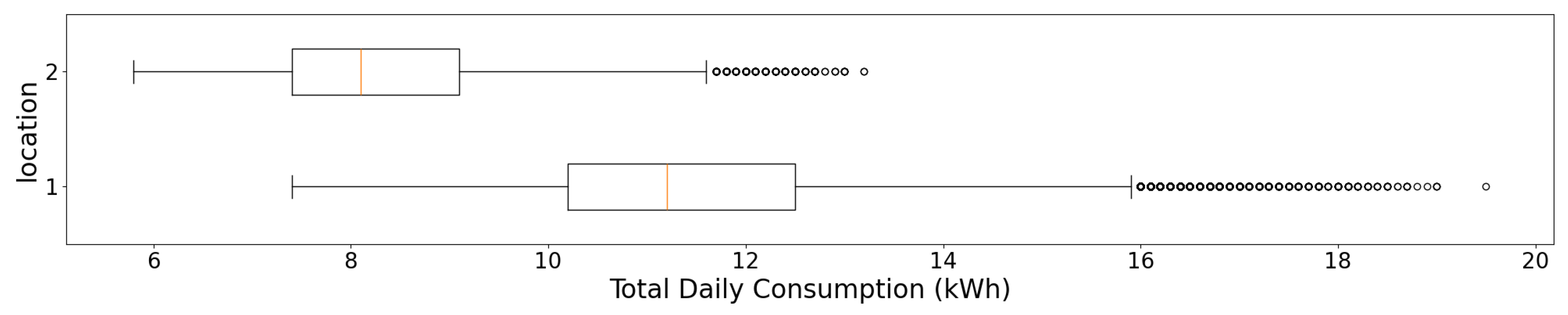
The synthetically generated dataset was examined to understand patterns in daily total energy consumption. Horizontal boxplots and associated descriptive statistics were produced for selected categorical variables: location, use of electric cooling, and season. Descriptive statistics include the number of observations, mean, standard deviation, minimum, quartiles, and maximum. For the variable location, the analysis shows that location 1 (‘house’) has a higher mean daily consumption $11.5$ (kWh) than location 2 (‘garden’, with $8.3$ kWh). The variability is also higher in location 1, with a standard deviation of $1.7$ kWh compared to $1.2$ kWh in location 2 (Figure 3).

Households with electric heating (e_heat $=1$) consume more on average ($11.2$ kWh; $Q1=9.9$, $Q2=11.0$, $Q3=12.5$) than those without ($10.73$ kWh; $Q1=9.6$, $Q2=10.7$, $Q3=11.9$). They also show slightly greater variability ($2.17$ kWh vs. $1.8$ kWh).

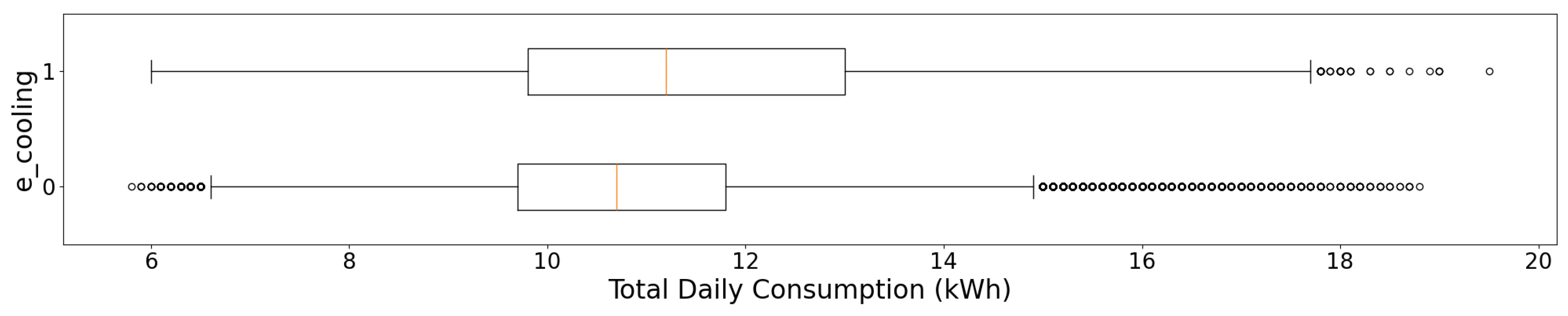
Electric cooling (e_cooling) is associated with higher daily consumption. Households without electric cooling have a mean of $1.8$ kWh, while those with electric cooling average $11.3$ kWh. The spread of values is also wider in the latter group (Figure 4).

Seasonal patterns are evident. Winter exhibits the highest average daily consumption (11.9 kWh), followed by summer ($11.5$ kWh), spring ($10.7$ kWh), and autumn ($9.5$ kWh). Winter also shows the largest variation, with a standard deviation of $2.3$ kWh, whereas autumn shows the lowest variability ($1.2$ kWh). The boxplots in Figure 5 illustrate these seasonal differences.

5. Time Series Analysis

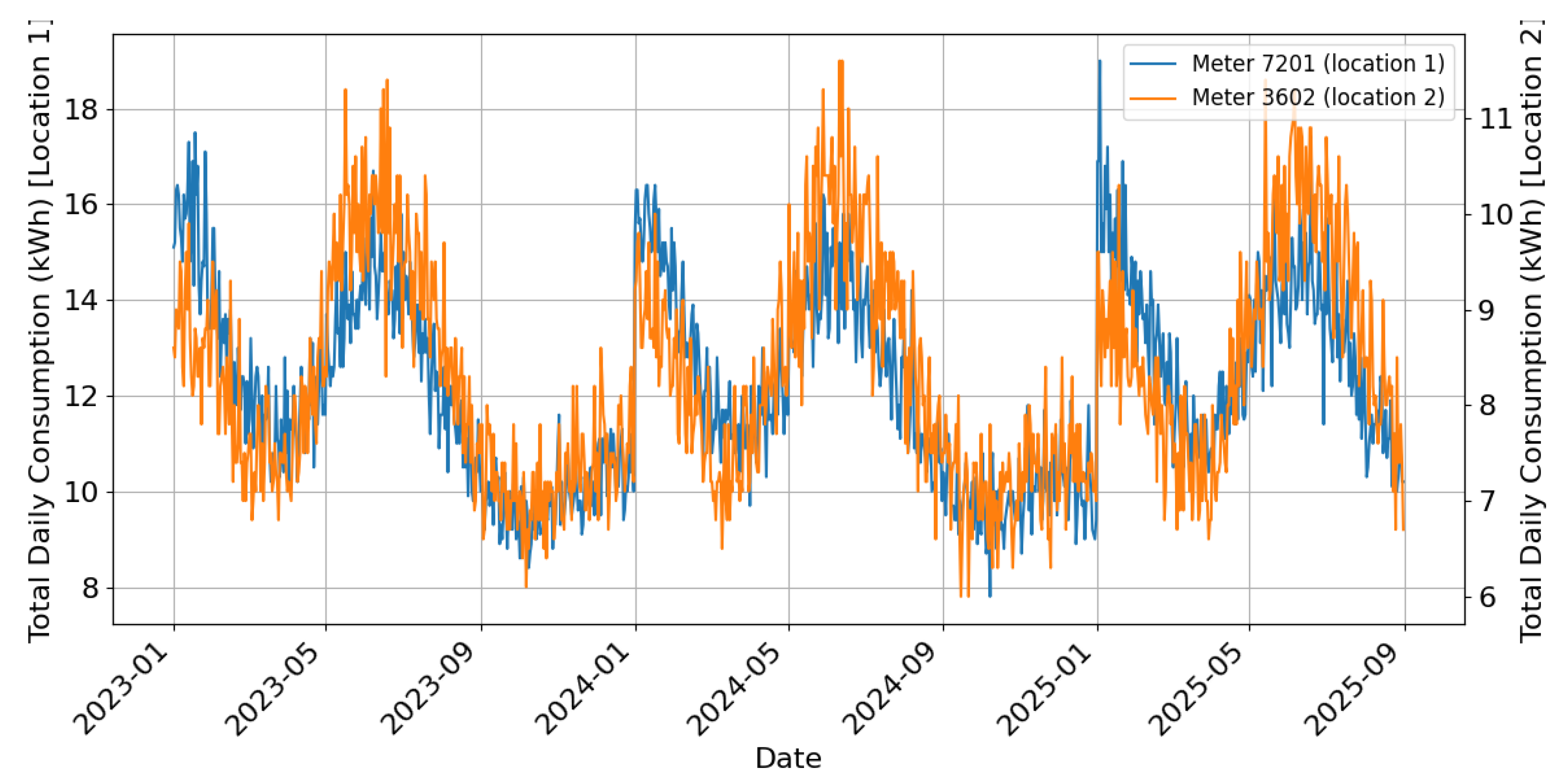
The dataset was analyzed at different temporal resolutions and aggregation levels in order to explore relevant characteristics and patterns in the structure of the time series. For this purpose, the energy consumption of each individual meter was represented at daily granularity. Figure 6 illustrates two representative daily consumption series, one from each location, displayed on a common timeline but with separate vertical axes. Although both series exhibit the same structure in terms of periodicity and the distribution of consumption peaks, a clear difference is observed in the overall daily consumption level, which is systematically higher for location 1.

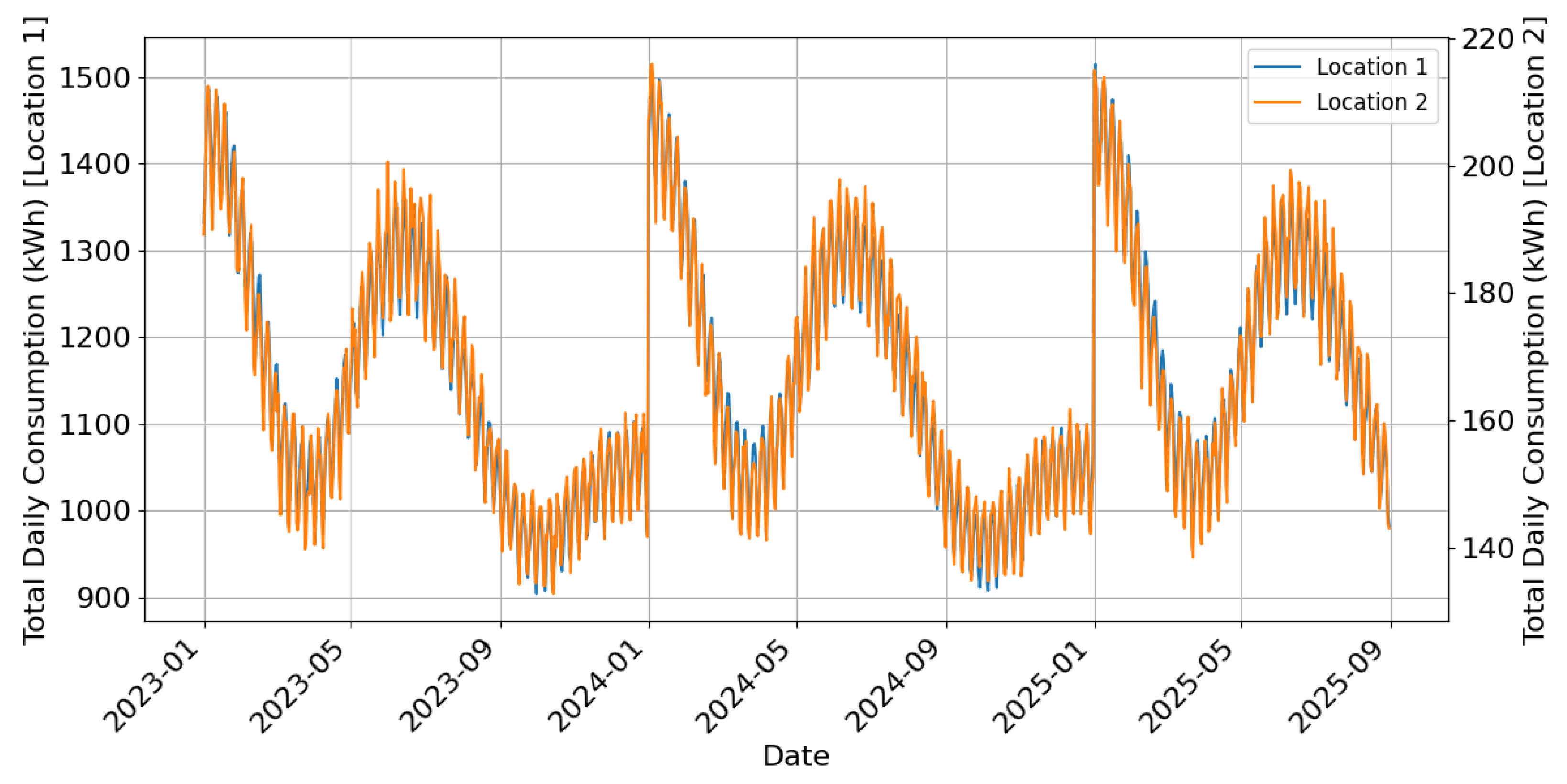
In addition, the same time series were visualized at the same temporal resolution, but aggregated across all meters within each category (location = 1 and location = 2). As shown in Figure 7, these time series exhibit a pronounced seasonal pattern with a weekly cycle superimposed. In addition, slower oscillations in the overall consumption level, likely related to seasonal effects, can be observed. The overall magnitude of consumption is consistently higher for location 1 compared to location 2, but the oscillation patterns and periodicity are the same in both cases.

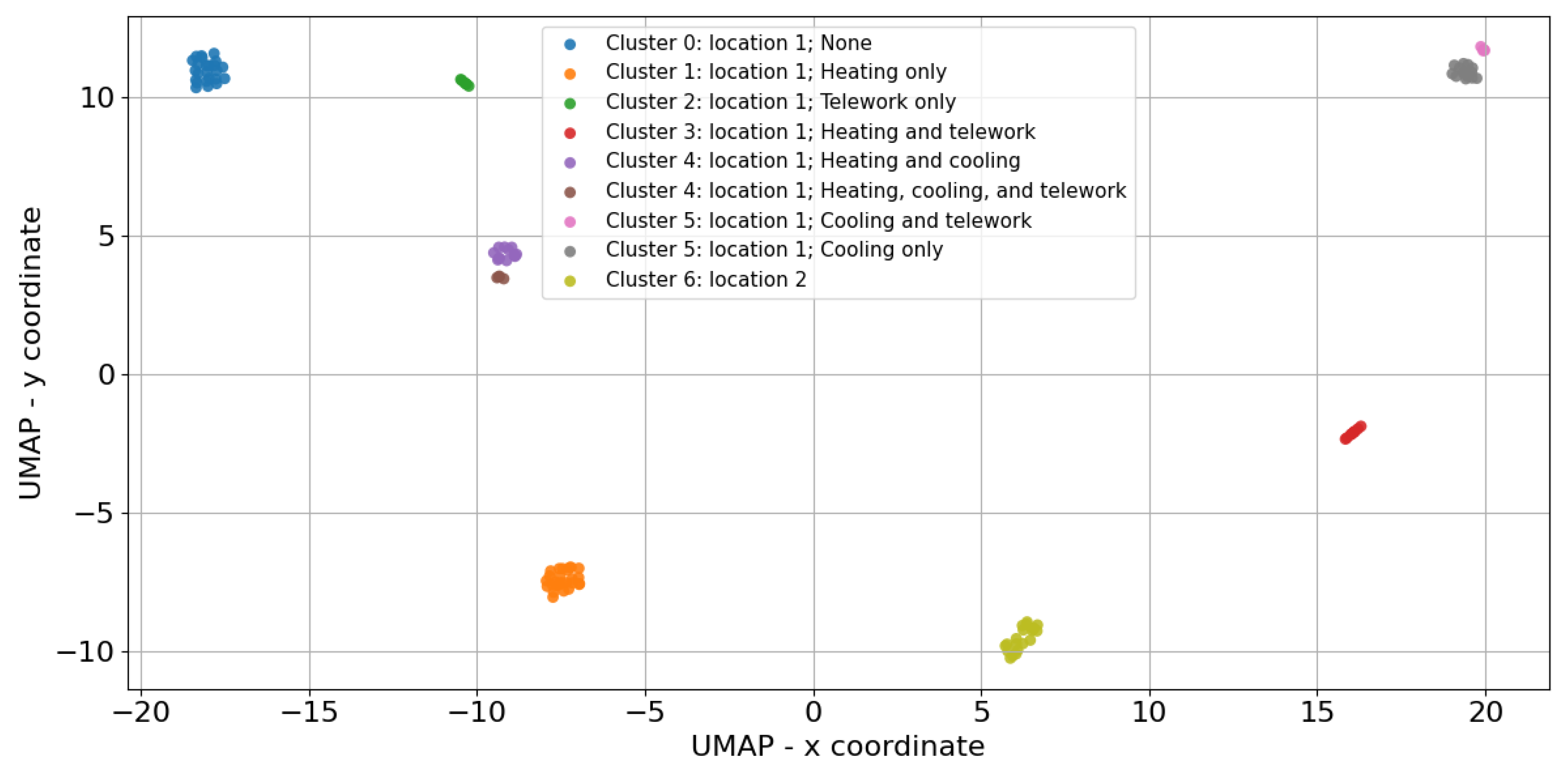
To investigate whether daily time series reveal distinct consumption patterns, we represented each meter by its complete daily sequence (974 values) and applied UMAP [32] to obtain a two-dimensional projection. The resulting map (Figure 8) shows, for each meter, its location, heating/cooling systems, telework status, and the cluster assigned by the method described below.

The visualization reveals one cluster grouping all meters with location = 2 (indicating that location dominates consumption behaviour in these cases) and six clusters for location = 1, where separation is mainly driven by heating, cooling, and telework attributes. Notably, customers with cooling + telework often merge with cooling only, while heating + cooling overlaps with heating + cooling + telework, suggesting that certain attribute combinations yield nearly identical profiles.

From Figure 8, we can deduce that the structure of the time series and the associated consumption patterns are primarily driven by four factors: meter location, telework, and the presence of heating and cooling.

In Figure 8, we can also analyse the clusters detected by a DBSCAN ($ϵ=0.8$, min_samples = 3) achieving a Silhouette Width score of $0.94$, indicating well-separated groups. Visual inspection of Figure 8 confirms that cluster structure closely follows customer characteristics. Section 6 further examines alternative clustering strategies for deeper segmentation.

6. Clustering Models

We use unsupervised learning to uncover recurring household consumption profiles and relate them to contextual factors (location, heating/cooling, telework) already shown to influence daily totals in prior sections. To capture the underlying grouping structure of the data, several clustering algorithms were evaluated, including hierarchical clustering [33], k-means [34], DIANA [35], PAM [36], CLARA [35], self-organizing maps (SOM) [37], the expectation-maximization (EM) algorithm over a finite mixture of Gaussian distributions (MODEL) [38], and self-organizing tree algorithm (SOTA) [39]. The objective is to obtain compact, well-separated, and interpretable clusters that remain stable across methods. Cluster quality was assessed using three internal validation metrics (Connectivity [40], Dunn Index [41], and Silhouette Width [42]), computed for cluster sizes between 3 and 10, jointly measuring compactness, separation, and stability.

Before clustering, the original customer–date–hour dataset was aggregated at the household level to enable grouping based on structural and behavioral characteristics. For each customer, summary statistics of key consumption and contextual variables were computed to capture both average behavior and variability, providing stable and comparable descriptors. The resulting feature set combined socio-demographic, structural, climatic, and behavioral indicators, including location (e.g., region, postal code), structural indicators (e.g., dwelling size, household composition), socio-economic variables (income, telework), and heating/cooling systems. Environmental effects were represented by daily maximum and minimum temperatures and solar radiation statistics, while consumption behavior was summarized by the mean and standard deviation of hourly loads. This integrated representation supports a meaningful segmentation of households into homogeneous groups.

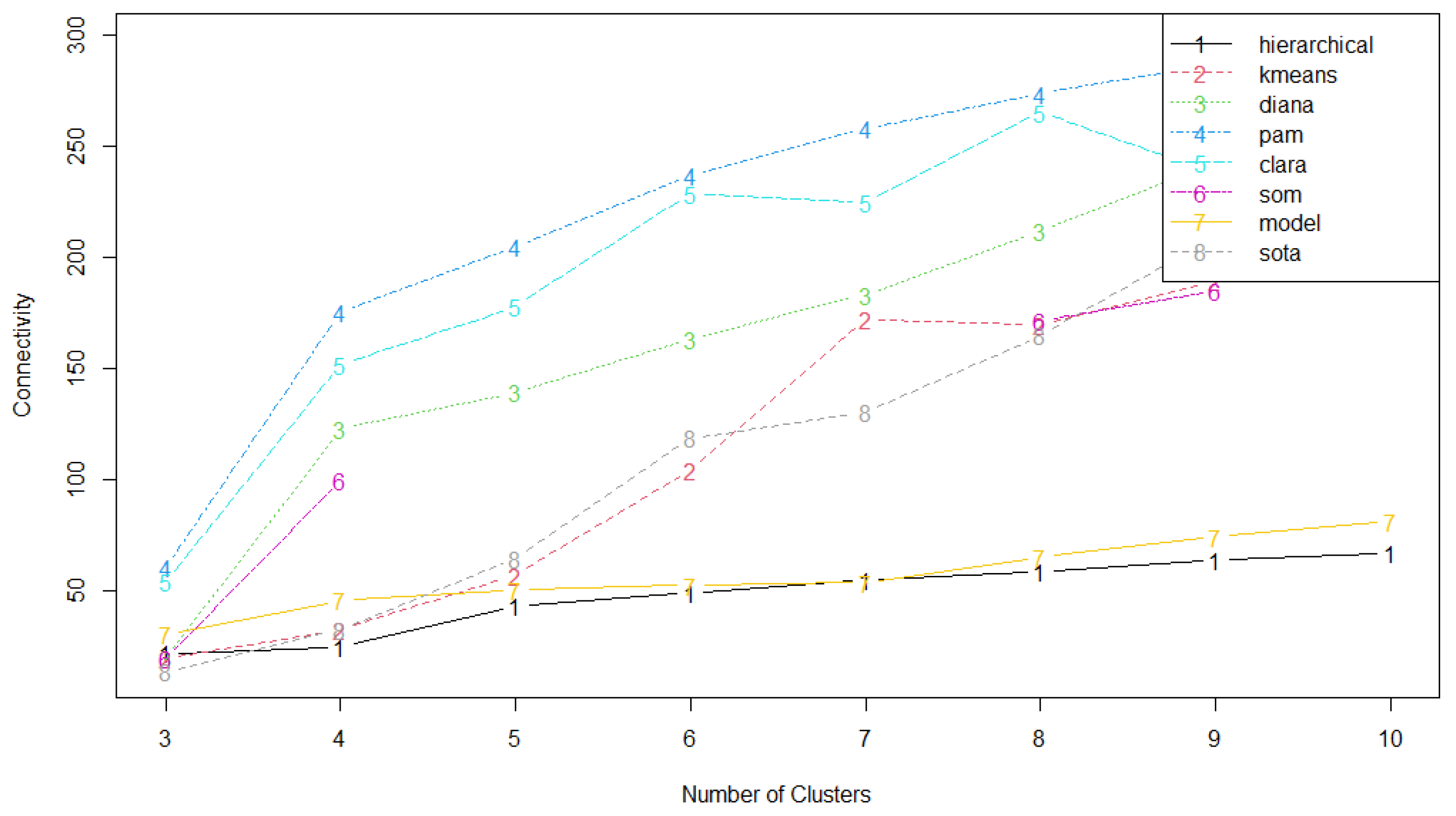
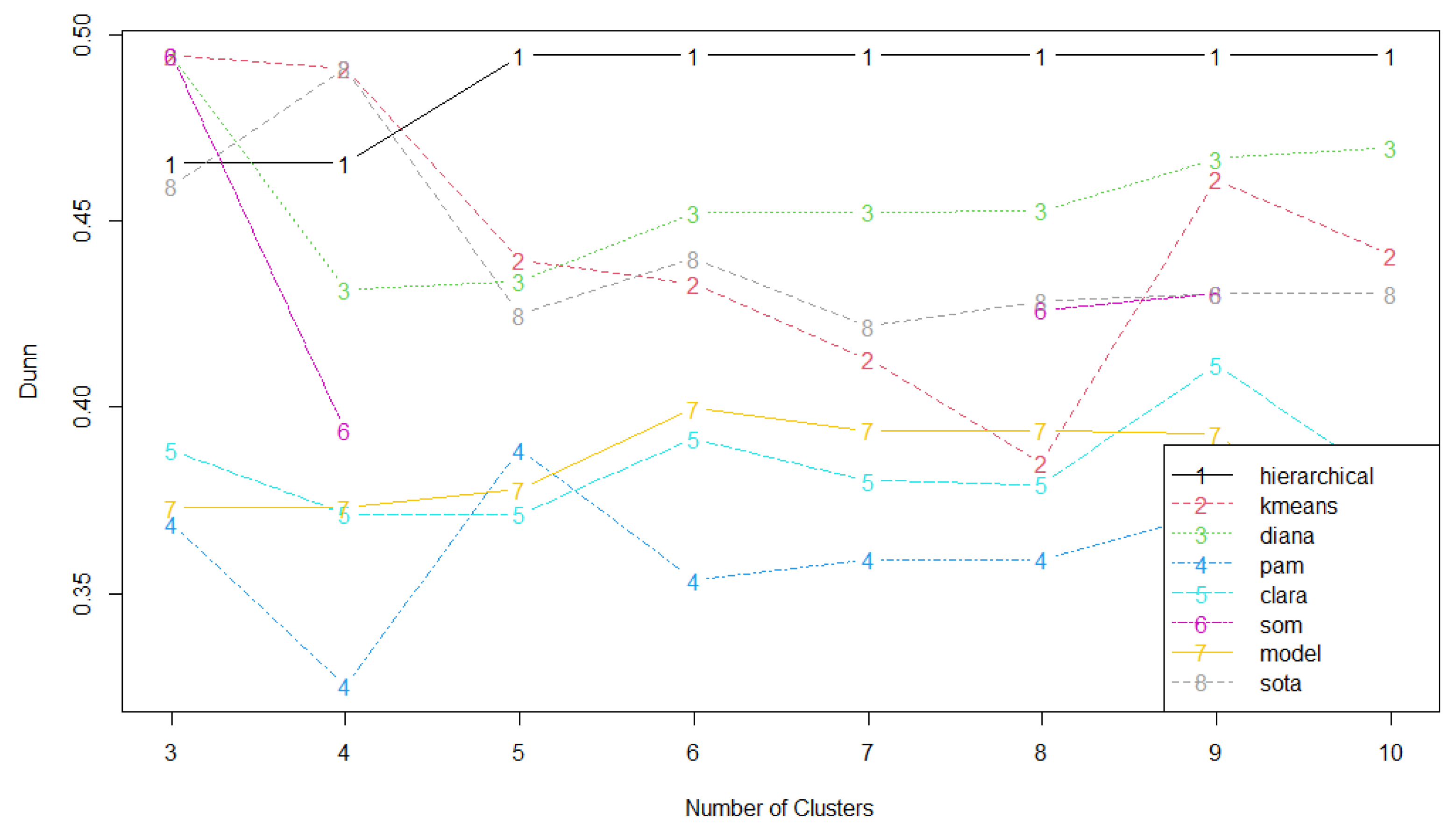
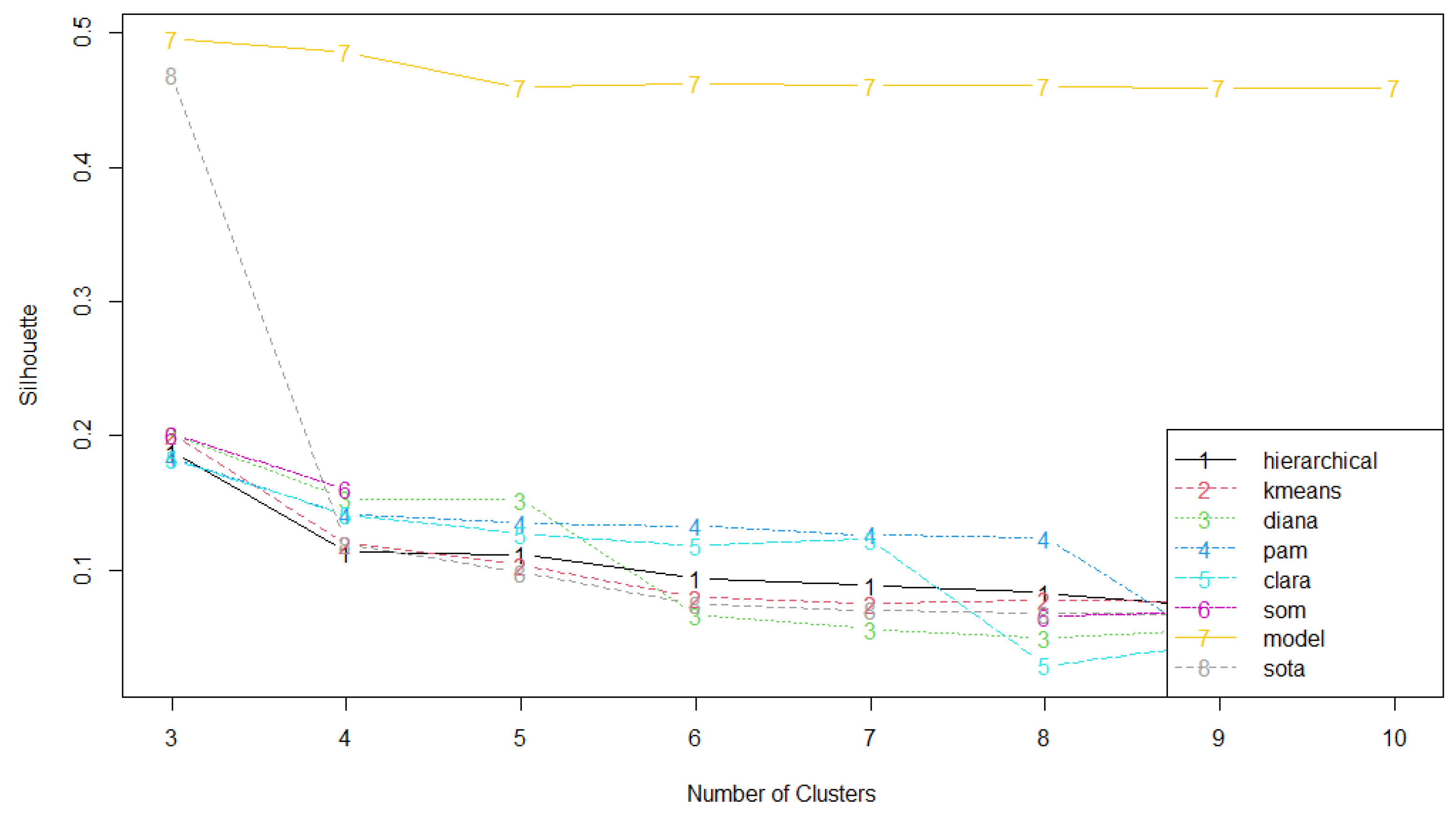
Figure 9, Figure 10 and Figure 11 summarize the validation results for the three internal metrics considered. Each figure reports the scores obtained for all algorithms across a range of cluster sizes (from 3 to 10), allowing a more detailed inspection of how the quality of the partitions evolves as the number of clusters increases. Connectivity scores show that hierarchical and k-means methods yield more coherent clusters for small k, whereas PAM and CLARA exhibit substantially higher values, indicating less well-structured groupings. The Dunn Index figure shows a more balanced landscape, with hierarchical, k-means, DIANA, and SOM achieving comparable performance at specific cluster sizes, whereas PAM and CLARA generally remain below the top performers. Silhouette Width highlights the model-based approach as the most consistent performer, achieving the highest values across configurations and indicating a favorable balance between cohesion and separation. Overall, these complementary metrics offer a comprehensive view of clustering quality and algorithmic trade-offs.

Table 2. Optimal Clustering Scores.

Score	Method	Clusters
Connectivity	SOTA	3
Dunn	Hierarchical	5
Silhouette	Model-based	3

summarizes the optimal validation results for each clustering algorithm. Connectivity measures how well the clusters are formed by penalizing instances that are placed far from their natural neighbors (lower values are better). The Dunn Index assesses cluster compactness and separation (higher values are better), while the Silhouette Width provides a normalized measure of cohesion and separation, ranging from $-1$ to 1 (higher values indicate better-defined clusters).

From the analysis, the SOTA method achieved the lowest Connectivity score (13.20) with three clusters, suggesting a well-structured partition. The highest Dunn Index (0.4945) was obtained by the hierarchical method with five clusters, highlighting its ability to identify compact and well-separated groups. Regarding Silhouette Width, the model-based approach outperformed the other methods, reaching 0.4955 with three clusters, which indicates a balanced trade-off between cohesion and separation of clusters.

Overall, no single clustering algorithm consistently outperformed the others across all metrics. Instead, the choice of method depends on the balance between compactness, separation, and interpretability. In this study, the model-based clustering with three clusters appears to provide the most coherent structure, although hierarchical clustering with five clusters and the SOTA approach with three clusters also delivered competitive results. These insights are relevant for further analysis of consumption patterns, where the identification of distinct user profiles may inform targeted strategies for energy efficiency.

7. Forecasting

For forecasting, we focus on the total daily electricity consumption of individual meters. As an example, we select a single meter and extract its daily consumption time series from the dataset. The last 90 days of the time series are reserved for validation and testing (30 days for validation and 60 days of testing), and the remaining observations are used for training. Household attributes (number of residents, children, adults, seniors, income) are incorporated as exogenous regressors, with missing values forward- and backward-filled. Although meteorological variables are generated as part of the synthetic data to induce realistic consumption patterns, they are not used as input features in the forecasting models. All forecasting experiments rely exclusively on historical consumption, calendar variables, and household-level contextual attributes.

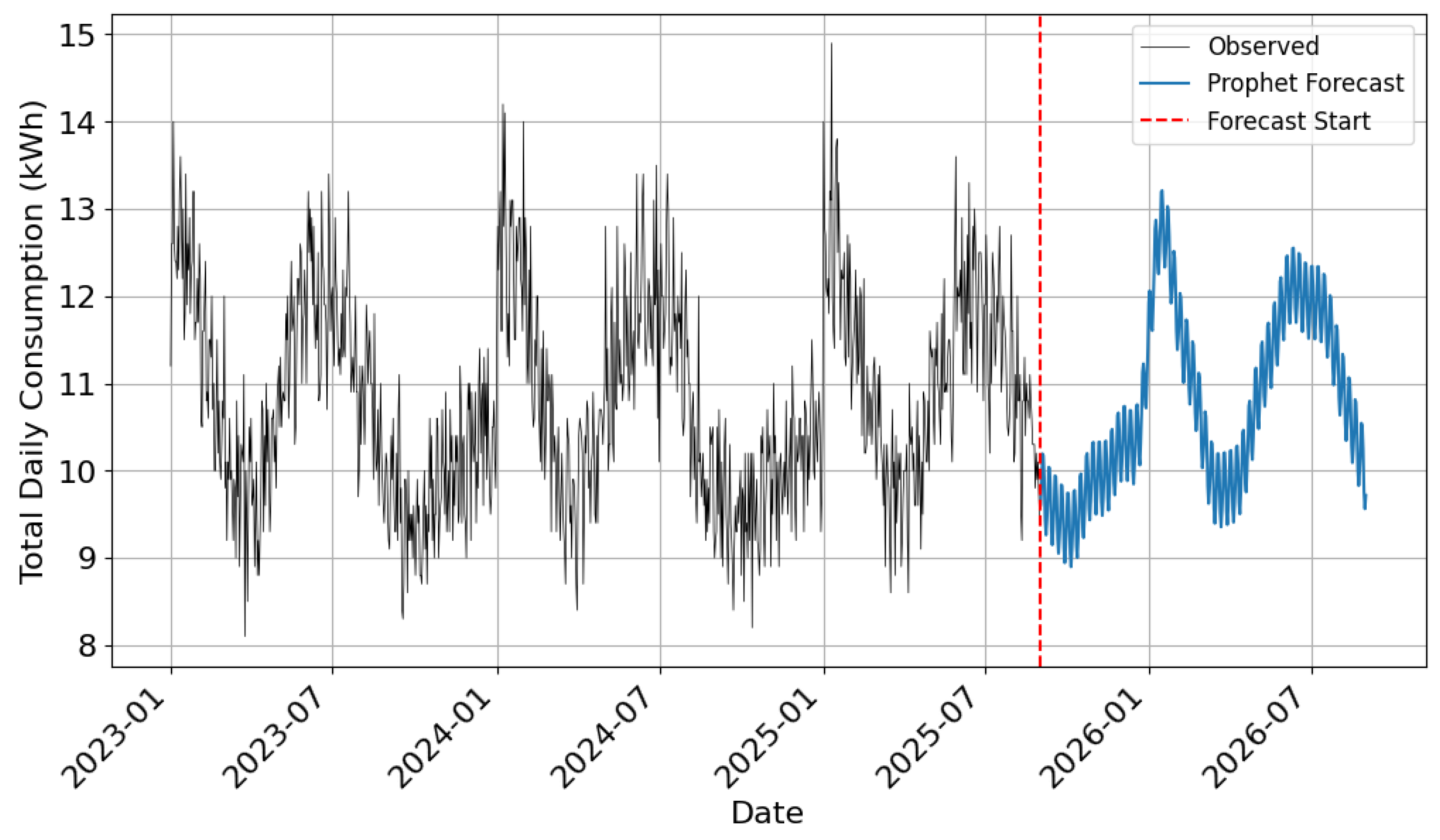
We first employ the Prophet model [43], configured with yearly and weekly seasonality and a flexible trend via a higher changepoint prior scale. Household features are included as additional regressors. The model is first fitted to the entire time series to generate a long-term forecast of 365 days. Figure 12 displays the forecasted series alongside the observed consumption to visually assess the quality and temporal alignment of the predictions.

For model evaluation, we fit a separate Prophet model using only the training set and evaluate the validation-set performance for hyperparameter tuning. Then, a model is trained using the training and validation sets together with the hyperparameters found. Forecasts are generated for the 60-day test period and compared against observed values using root mean squared error (RMSE), mean absolute error (MAE), mean absolute percentage error (MAPE), and weighted mean absolute percentage error (WMAPE). RMSE and MAE are expressed in the same units as the target variable, which in this case is total daily electricity consumption measured in kilowatt-hours (kWh), whereas MAPE and WMAPE are reported as percentages. For the selected meter, the resulting RMSE ($0.54$ kWh), MAE ($0.43$ kWh), MAPE ($3.99\%$), and WMAPE ($3.94\%$) indicate the predictive accuracy of the model.

To benchmark against a non-autoregressive model, we train a LightGBM regressor under the same experiment setup. The model is configured with a learning rate of 0.001, 27 leaves per tree, and a minimum of 5 samples per leaf, optimizing a regression objective with RMSE as the evaluation metric; early stopping with a patience of 50 boosting rounds is applied to select the optimal number of iterations. The features used include the following:

• Temporal context variables, such as the day of the month, the month, and the day of the week on which the prediction is made.
• Lag-based variables are included, comprising lags of the previous day, two days before, one, two, and three weeks before, as well as one month, two months, and one year before.
• Aggregation variables are added, where the maximum, minimum, and mean are calculated for the lag periods of 1–7 days, 7–14 days, 1–30 days, 31–60 days, 61–90 days, 90–180 days, and 181–365 days.

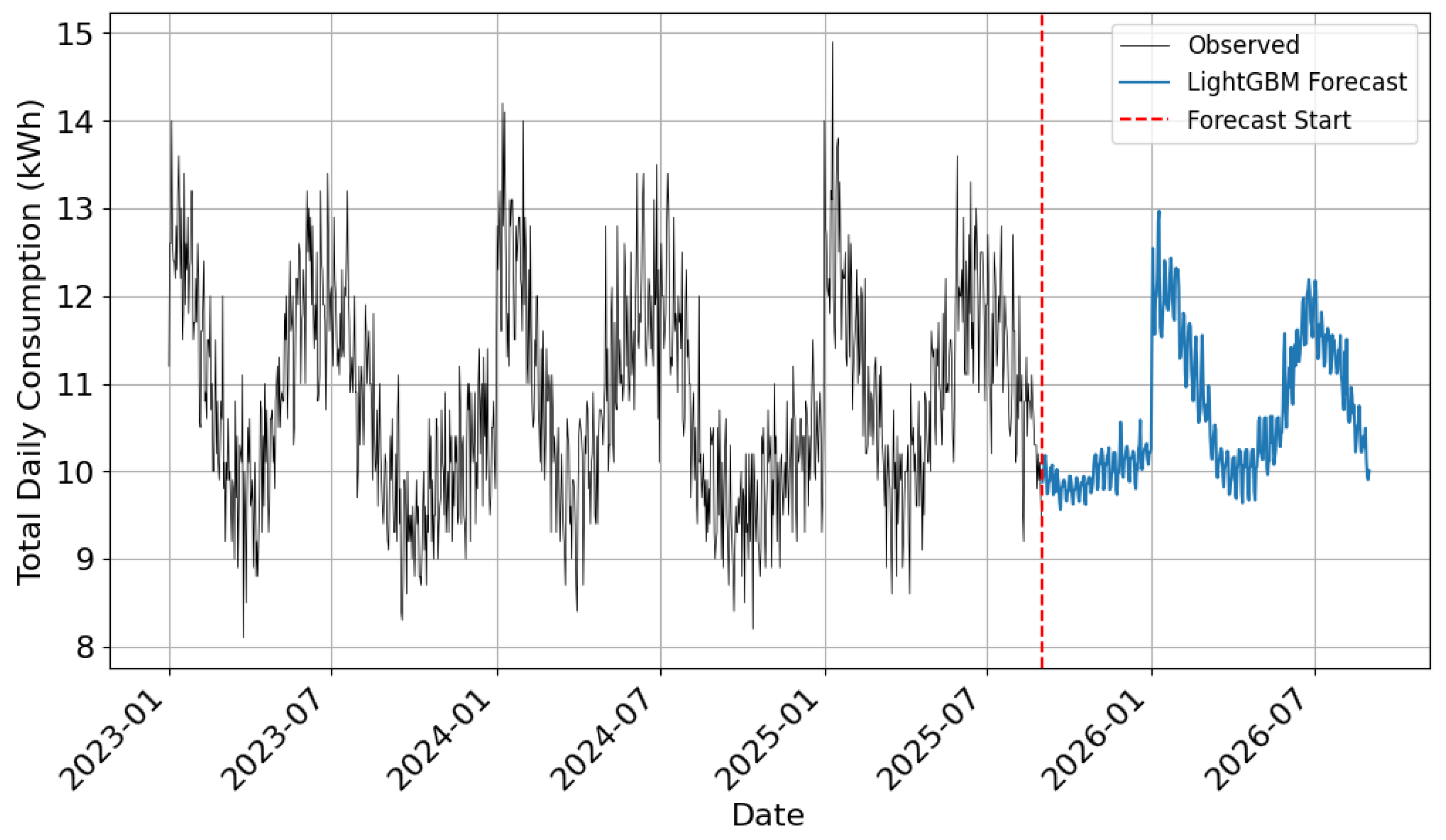
LightGBM achieves RMSE $=0.54$ kWh, MAE $=0.42$ kWh, MAPE $=3.89\%$, and WMAPE $=3.86\%$, slightly outperforming Prophet. This improvement can be attributed not only to LightGBM’s ability to capture nonlinear relationships and interactions among exogenous variables, but also to the inclusion of autoregressive features with specific lags and aggregated variables over defined time windows, which enrich the temporal signal available to the model. In Figure 13, the model’s forecasts for the following 365 days are displayed to evaluate the quality of the predictions.

To ensure a transparent and consistent comparison between Prophet and LightGBM, both models were trained and evaluated under the same experimental protocol. The time series was partitioned into training, validation, and test sets of identical length for both models (519 days for train, 30 days for validation and 60 days for test), and each model had access to the same exogenous information. Model selection was performed using the validation set, where hyperparameters were tuned to minimise standard forecasting error metrics (RMSE, MAE, MAPE and WMAPE). After selecting the best configuration, each model was retrained on the combined training and validation data and finally evaluated on the held-out test period. This common evaluation framework ensures that differences in performance reflect the intrinsic modelling capabilities of each method rather than differences in data access or training regime. Under these controlled conditions, LightGBM systematically outperforms Prophet across all evaluation metrics.

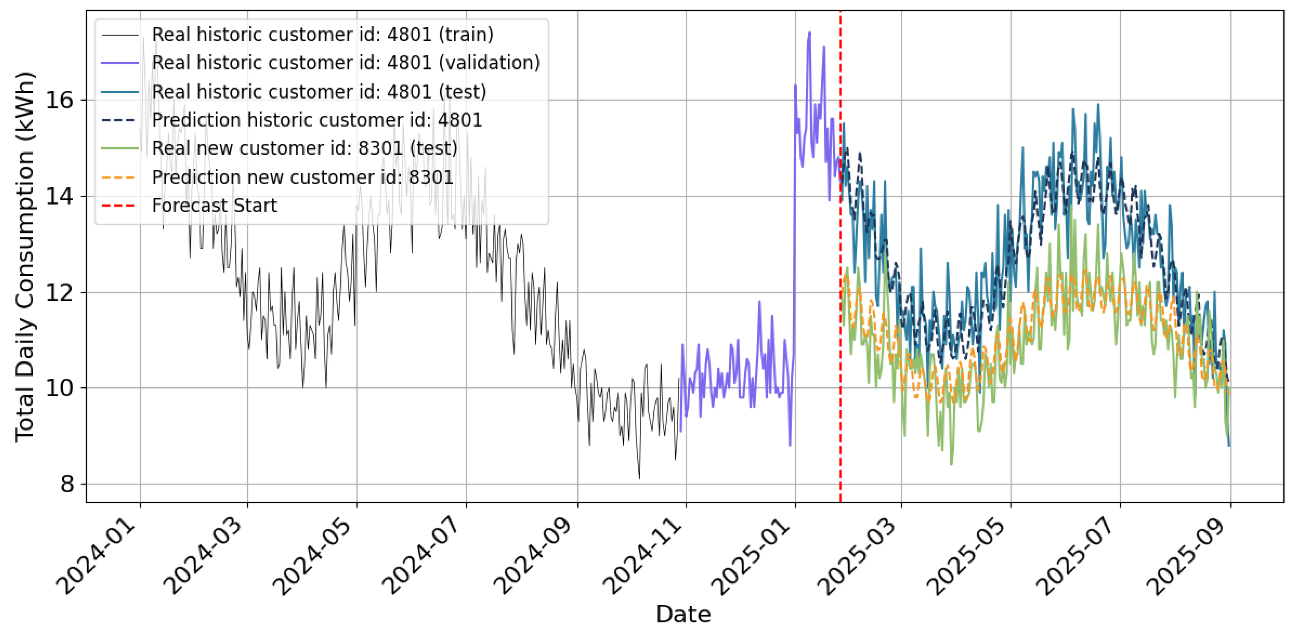
To extend the evaluation to a multi-series setting, an experiment was designed to address the cold-start problem for new customers. Data are split into 10 months for training: 3 for validation, and 7 for testing. The dataset comprises 100 m at location 1 and 20 m at location 2. From each location, 20% of the meters are randomly selected and treated as newcomers, and are therefore excluded entirely from both the training and validation sets. The remaining meters at each location are used to train the forecasting models using the data available for the specified training and validation periods. Separate models are fitted for locations 1 and 2, using a LightGBM regression configuration with a learning rate of 0.07, 28 leaves per tree, and a minimum of 7 samples per leaf, optimizing RMSE; early stopping with a patience of 50 boosting rounds on the validation set is used to select the optimal number of iterations, with early stopping based on validation performance.

Model performance was subsequently assessed on the test set, and an additional prediction was generated for future periods. Because part of the feature set relied on lagged consumption values, a clustering-based imputation strategy was employed for customers without historical records. Specifically, historical customers were characterized by the binary attributes location, telework, e-heating, and e-cooling, and grouped into clusters whose centroids were defined by the mean attribute values. New customers were assigned to the nearest centroid, and their lag-based features were reconstructed using the mean of historical values of the corresponding cluster. After testing different clustering methods and based on the results in Table 2, the best performance for the consumption prediction of new customers was achieved using hierarchical clustering with five clusters.

The evaluation results (

Table 3. Forecasting performance for historical and new customers across locations.

	RMSE (kWh)		MAE (kWh)		MAPE (%)		WMAPE (%)
	Loc. 1	Loc. 2	Loc. 1	Loc. 2	Loc. 1	Loc. 2	Loc. 1	Loc. 2
Historical customer	0.64	0.51	0.51	0.4	4.33	4.74	4.33	4.76
New customer	1.03	0.87	0.77	0.69	6.11	7.7	6.4	8.0

) show higher errors for new customers, as expected given that their lagged features are reconstructed from cluster-level averages rather than own histories.

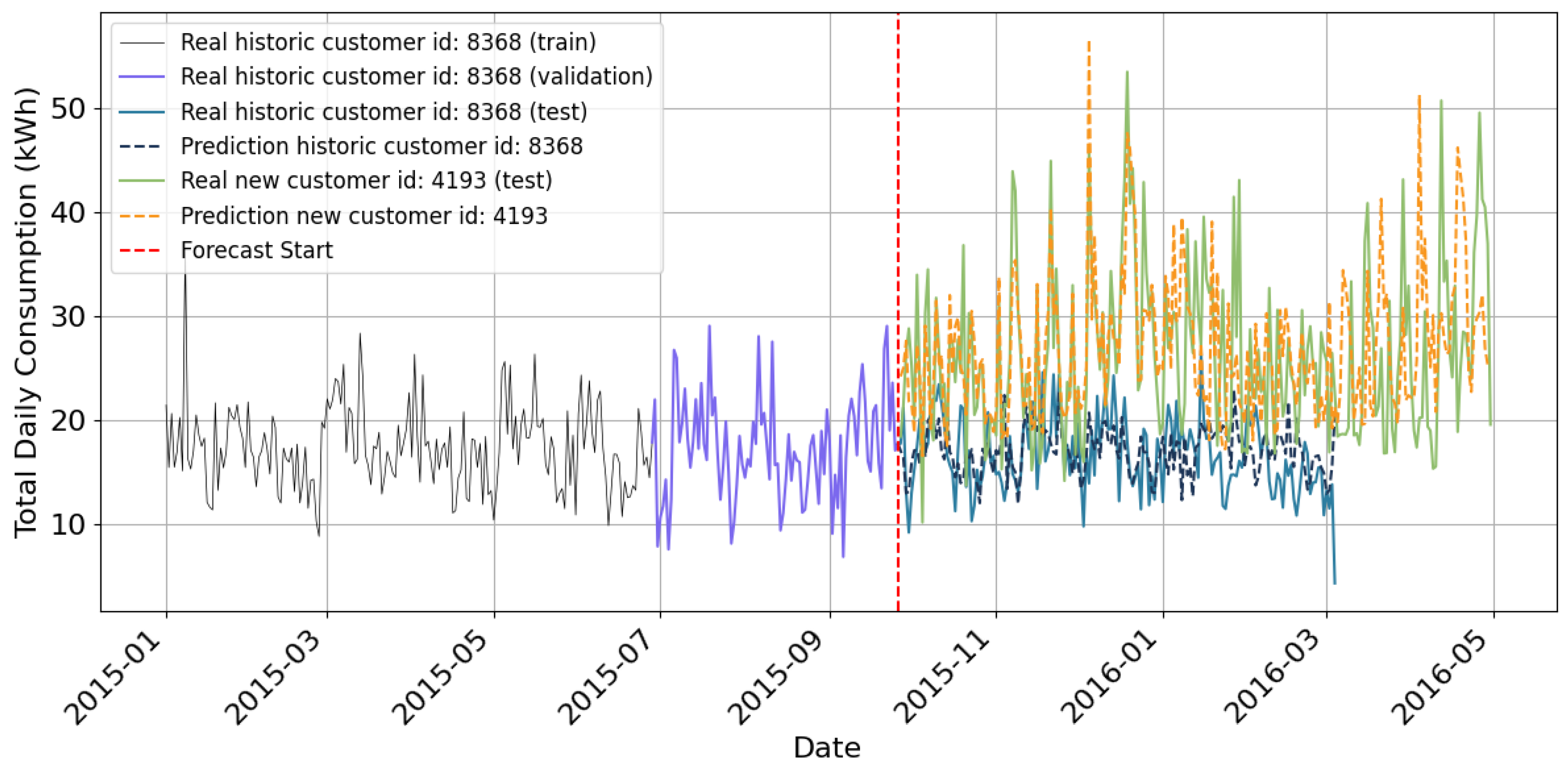
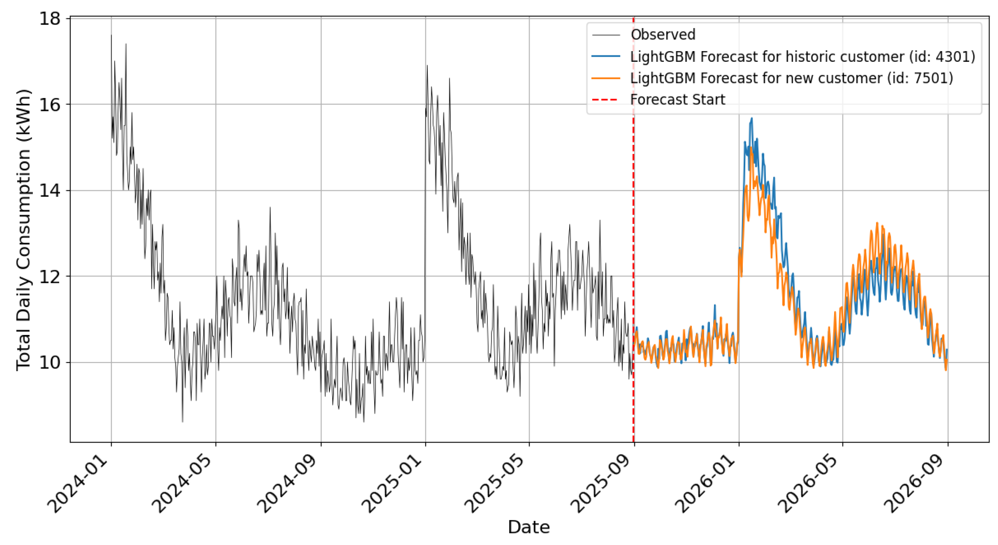
To further analyze how forecasting accuracy evolves over time, prediction errors were also evaluated as a function of the forecasting horizon. Starting from a given reference date in the test period, forecasts were generated recursively over an extended horizon, with lag-based inputs progressively updated using the model’s own predictions. The weighted mean absolute percentage error (WMAPE) was computed separately for four horizon windows: short-term (1–7 days), short-to-medium term (7–31 days), medium-term (31–180 days), and long-term (180–217 days). The resulting WMAPE values were 4.51%, 4.29%, 4.41%, and 4.36% for historical customers and 6.32%, 5.89%, 7.01%, and 5.21% for new customers, corresponding to the 1–7, 7–31, 31–180, and 180–217 day horizons, respectively.

Figure 14 presents the corresponding future forecasts. Figure 15 and Figure 16 report test-period results for meters at locations 1 and 2, respectively. The results show a poorer fit for new customers at location 2 than at location 1, plausibly due to pronounced data imbalance (location 1 has roughly five times as many series) and the cold-start setting for new customers, which together degrade performance in the absence of individual historical values.

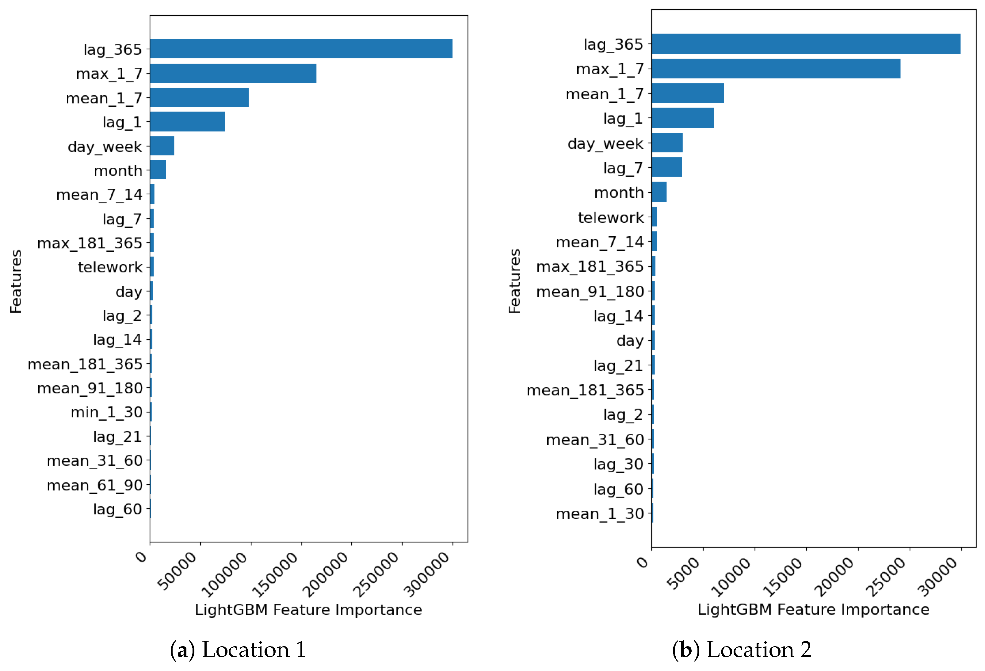
With the aim of gaining a deeper understanding of the dependencies present in the data, feature importance derived from the LightGBM models of the multi-series forecasting setting is reported in Figure 17. This analysis shows consistent patterns across locations. The 365-day lag is the most influential feature, confirming strong annual periodicity, followed by recent-week aggregates (max/mean over last 7 days), reflecting stable short-term consumption dynamics.

The proposed framework can be used to anticipate peak loads and design demand response strategies, including forecasting consumption for new customers and planning supply under cold-start conditions.

To quantify the contribution of contextual variables and cluster-informed lag reconstruction, another experiment was carried out in which all socio-demographic and household-level attributes were removed from the feature set. In this setting, no clustering step can be applied because clusters cannot be assigned to new customers and, consequently, lag-based features for new customers cannot be reconstructed from their assigned cluster. Instead, lagged values are approximated using global aggregations. Moreover, separate models per location cannot be used, so a single LightGBM is trained for locations 1 and 2.

Table 4. Forecasting performance for historical and new customers across locations without contextual information.

	RMSE (kWh)		MAE (kWh)		MAPE (%)		WMAPE (%)
	Loc. 1	Loc. 2	Loc. 1	Loc. 2	Loc. 1	Loc. 2	Loc. 1	Loc. 2
Historical customers	0.64	0.53	0.51	0.42	4.34	4.91	4.36	4.93
New customers	1.47	2.57	1.13	2.47	8.82	29.79	9.41	28.83

reports the corresponding forecasting performance. For historical customers, the absence of contextual information and the lack of a location-specific model leads to a slight deterioration in accuracy for meters at location 1 where, for example, WMAPE increases from $4.33$% to $4.36$%, and a large deterioration for meters is observed in location 2, where WMAPE increases from $4.76$% to $4.93$%. For new customers, the degradation is substantially larger (e.g., WMAPE rises from $6.40$% to $9.41$% at location 1 and from $8.00$% to $28.83$% at location 2). These results highlight that contextual variables and the derived clustering structure are crucial to obtain accurate predictions, especially in cold-start scenarios where no individual consumption history is available. Overall, the model without contextual information and clustering yields markedly worse performance, confirming the practical value of the proposed pipeline design.

Testing on Real Data

To assess the applicability of the proposed methodology beyond the synthetic setting, we conducted an additional experiment using an extended version of the Pecan Street dataset available on Kaggle [30].

The dataset consists of electricity consumption records from multiple residential customers. The original measurements were aggregated to daily resolution, yielding a single time series of total daily energy consumption (kWh) per customer. This aggregation ensures consistency with the forecasting target used throughout the paper. From the daily series, we derived the same family of temporal features as in the synthetic experiments, including calendar variables, lagged consumption values, and rolling-window statistics. No explicit socio-demographic or dwelling-related attributes are available in this dataset.

To replicate a realistic forecasting scenario with unseen users, 20% of the customers were randomly selected as newcomers and excluded entirely from both training and validation. The remaining customers were used to construct consumption-based representations, perform clustering, and train the forecasting models. As in the synthetic setting, clustering was applied at the customer level in order to identify homogeneous consumption profiles. Instead of training a single global model, one forecasting model per cluster was learned, allowing each model to specialize in a specific consumption pattern.

Due to the absence of contextual variables describing household or dwelling characteristics, cluster assignment for newcomers cannot be performed using static attributes. In this experiment, newcomers were therefore assigned to clusters based on the similarity of their electricity consumption patterns observed during the training period. Although, by definition, true newcomers would not have historical consumption records available at onboarding time, this assumption allows us to analyze a controlled what-if scenario in which new customers can be perfectly or near-perfectly assigned to their most representative consumption cluster. Specifically, each newcomer was matched to the cluster whose representative consumption profile exhibited the highest similarity to its own, thereby providing an upper-bound estimate of the forecasting performance that can be achieved when cluster membership is correctly identified.

After cluster assignment, forecasts for the test period were generated using the corresponding cluster-level models. Performance was evaluated using the same metrics as in the synthetic experiments (RMSE, MAE, MAPE, and WMAPE).

Table 5. Forecasting performance for historical and new customers of the Pecan Street Dataset.

	RMSE (kWh)	MAE (kWh)	MAPE (%)	WMAPE (%)
Historical customers	9.07	5.21	26.5	22.18
New customers	14.57	6.04	30.93	25.27

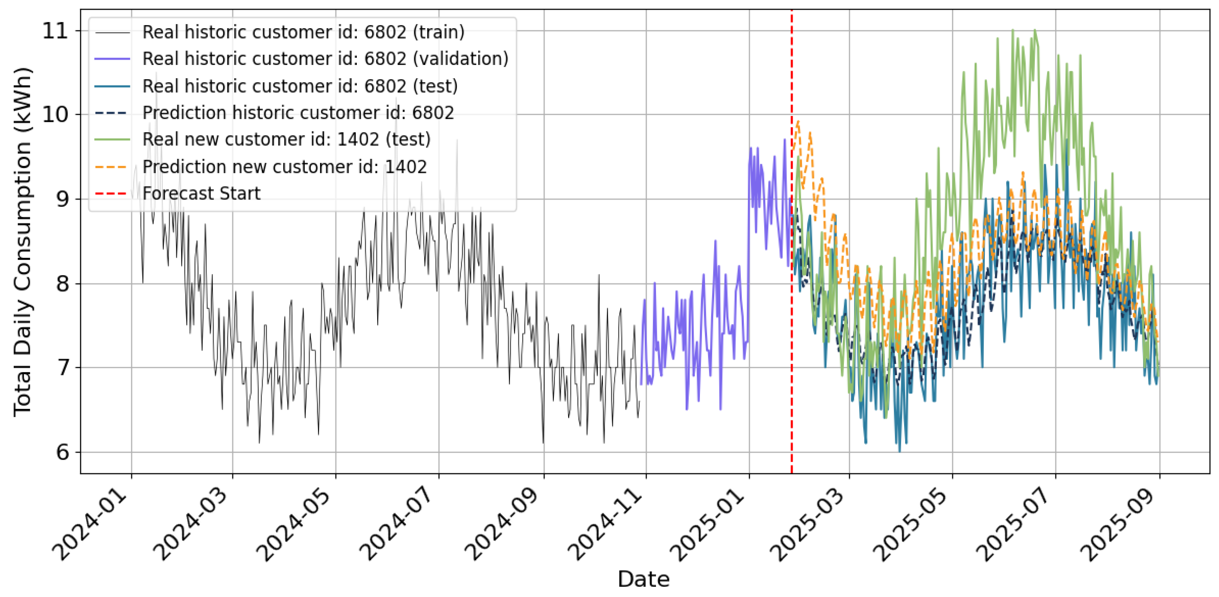
summarizes the results separately for customers with historical data used in training and for newcomers. Figure 18 illustrates representative forecasts compared with observed values over the test horizon, highlighting differences in predictive accuracy between customers with full historical information and newcomers.

Following the same recursive forecasting protocol and horizon-based evaluation strategy defined for the synthetic experiments, prediction errors were also analyzed as a function of the forecasting horizon on real data. Forecasts were generated over a total horizon of seven months (217 days), and the weighted mean absolute percentage error (WMAPE) was computed separately for four horizon windows: 1–7, 7–31, 31–180, and 180–217 days. The resulting WMAPE values were 14.46%, 14.78%, 22.17%, and 32.72% for historical customers, and 16.81%, 20.97%, 24.56%, and 36.59% for new customers, respectively. Forecasting accuracy decreases as the prediction horizon increases, with the lowest errors observed in the short-term window and a gradual degradation for longer horizons, which is more pronounced for new customers due to the cold-start condition.

As shown by the metrics reported in Table 5, forecasting errors on real data are higher than those obtained on the synthetic dataset, as expected. Although the model is able to capture the overall trend and seasonal structure of the time series, it exhibits larger deviations around some peak consumption events that are difficult to anticipate from historical information alone. Nevertheless, the results show a strong performance for new customers, with only a limited degradation compared to customers with historical data. This indicates that the proposed framework generalizes well to real-world settings and that the cluster-informed feature reconstruction strategy provides an effective mechanism for mitigating the cold-start problem when individual consumption histories are unavailable.

8. Conclusions & Future Work

This work presented a three-stage methodological pipeline that integrates descriptive analysis, unsupervised segmentation, and forecasting, applied to synthetically generated household electricity data. The main contribution of this study is methodological: it provides an integrated and reproducible framework that clarifies when contextual information and segmentation improve forecasting performance, particularly in cold-start scenarios. The approach enables a systematic understanding of energy consumption behavior by linking temporal patterns, consumer typologies, and predictive models within a single framework. The use of synthetic data allowed full control over structure, variability, and reproducibility, while capturing realistic features of household demand such as seasonal cycles, daily routines, and behavioral heterogeneity. This design also made it possible to explicitly evaluate the impact of contextual variables and clustering on forecasting performance under controlled conditions, something difficult to achieve using existing public datasets that lack detailed household information or are subject to access restrictions.

The descriptive stage provided insights into the temporal structure of consumption, confirming consistent seasonal variation and the influence of household and environmental factors. The clustering stage identified coherent user segments driven mainly by location, heating and cooling systems, and telework status. These factors are not strictly orthogonal, as the same socio-economic conditions that favor the presence of heating and cooling systems may also influence telework status in real-world scenarios. Nevertheless, they reflect the main attributes identified by the segmentation as drivers of consumption patterns. These findings demonstrate that simple contextual and demographic attributes can explain substantial differences in consumption behavior. The forecasting stage showed that models using autoregressive and contextual features achieve accurate predictions for both existing and new customers. LightGBM outperformed Prophet across all error metrics, suggesting that tree-based ensemble models are more effective in capturing nonlinear dependencies in this type of data. Moreover, integrating cluster-based information improved forecasts for new customers with no historical data, partially mitigating the cold-start problem. A complementary experiment without contextual variables showed a substantial degradation in accuracy, especially for new customers, confirming that both segmentation and context-aware lag reconstruction play a central role in forecasting performance.

In addition to the synthetic experiments, the evaluation on real-world data using the Pecan Street dataset provides further evidence of the practical relevance of the proposed methodology. Although forecasting errors increase in the real-data setting the framework is able to capture the main temporal patterns and delivers competitive performance for new customers. A more detailed inspection of the results using relative error metrics such as MAPE and WMAPE, which are suitable for cross-dataset comparison, reveals that the relative performance gap between customers with historical data and new customers is smaller on real data than in the synthetic setting. This suggests that the higher intrinsic variability and unobserved heterogeneity of real-world consumption partially reduce the advantage of long individual histories, while the cluster-based structure still provides a stabilizing effect in cold-start scenarios. These results support the external validity of the proposed pipeline and suggest that the methodological insights derived from the synthetic experiments translate to realistic scenarios.

Overall, the results illustrate that the proposed framework can support several operational and analytical tasks, including demand forecasting, consumption profiling, and scenario simulation. Its modular design allows the integration of additional components, such as real-time monitoring or adaptive control, which could be relevant for utilities and policy makers. The interpretability of the models facilitates the identification of the main drivers of energy use, which is essential for designing effective energy management and demand response strategies. In addition, the synthetic dataset and the full pipeline are publicly released, enabling reproducible experimentation and offering a flexible benchmark for evaluating new forecasting or clustering approaches.

Further research will explore hybrid modeling approaches that combine tree-based and recurrent neural network models to capture both feature interactions and temporal dependencies. Additional efforts could also be directed toward improving the generation of synthetic data by incorporating socioeconomic variability and appliance-level profiles. Finally, interpretability methods such as SHAP or partial dependence analysis could be extended to identify regional or demographic differences in consumption behavior and to support the design of targeted energy efficiency programs.

Regarding the cold-start scenario, the present work relies on a simple and interpretable imputation strategy that assigns new customers to cluster centroids and reconstructs lag-based features using cluster-level averages. This choice was made to maintain transparency and to clearly assess the role of contextual variables and segmentation in forecasting performance, while this approach already yields substantial improvements over context-free baselines, it represents a coarse approximation of uncertainty in cold-start settings. Future work will therefore investigate more advanced alternatives, such as hierarchical Bayesian pooling, multi-task learning, or probabilistic imputation methods, which may further improve robustness and accuracy when limited or no historical data are available.

With respect to real-world data, future work will focus on improving forecasting accuracy by enriching the pipeline with additional sources of contextual information, such as neighborhood-level aggregates, or inferred dwelling characteristics. Further research will also explore more flexible strategies for assigning new customers to clusters, including probabilistic or soft assignment methods, as well as hierarchical or multi-task learning approaches that allow information sharing across heterogeneous customer groups. These extensions aim to better capture the complexity and variability of real consumption patterns while preserving the interpretability and modularity of the proposed framework.