Article

MVSegNet: A Multi-Scale Attention-Based Segmentation Algorithm for Small and Overlapping Maritime Vessels

by
Zobeir Raisi
*,
Valimohammad Nazarzehi Had
,
Rasoul Damani
and
Esmaeil Sarani
Electrical Engineering Department, Chabahar Maritime University, Chabahar 9971778631, Iran
*
Author to whom correspondence should be addressed.
Algorithms 2026, 19(1), 23; https://doi.org/10.3390/a19010023 (registering DOI)
Submission received: 20 November 2025 / Revised: 12 December 2025 / Accepted: 16 December 2025 / Published: 25 December 2025

Abstract

Current state-of-the-art (SoTA) instance segmentation models often struggle to accurately segment small and densely distributed vessels. In this study, we introduce MAKSEA, a new satellite imagery dataset collected from the Makkoran Coast that contains small and overlapping vessels. We also propose an efficient and robust segmentation architecture, namely MVSegNet, to segment small and overlapping ships. MVSegNet leverages three modules on the baseline UNet++ architecture: a Multi-Scale Context Aggregation block based on Atrous Spatial Pyramid Pooling (ASPP) to detect vessels with different scales, Attention-Guided Skip Connections to focus more on ship relevant features, and a Multi-Head Self-Attention Block before the final prediction layer to model long-range spatial dependencies and refine densely packed regions. We evaluated our final model with SoTA instance segmentation architectures on two benchmark datasets including LEVIR_SHIP and DIOR_SHIP as well as our challenging MAKSEA datasets using several evaluation metrics. MVSegNet achieves the best performance in terms of F1-Score on LEVIR_SHIP (0.9028) and DIOR_SHIP (0.9607) datasets. On MAKSEA, it achieves an IoU of 0.826, improving the baseline by about 7.0%. The extensive quantitative and qualitative ablation experiments confirm that the proposed approach is effective for real-world maritime traffic monitoring applications, particularly in scenarios with dense vessel distributions.

1. Introduction

Automated vessel detection and segmentation is one of the essential components of modern maritime surveillance within remote sensing. It has several applications in maritime security, environmental monitoring, and global logistics management. These tasks enable precise interpretation of satellite and aerial imagery for applications such as illegal fishing detection, maritime traffic analysis, port monitoring, and search and rescue operations [1,2,3,4,5].
High-resolution satellite imagery has become increasingly accessible in recent years. Therefore, automatic ship segmentation has become an active research topic in both the computer vision and remote sensing communities [6]. However, segmenting ships in optical satellite images remains highly challenging due to three factors: (1) small object scale, as ships often occupy less than 0.1% of the image area; (2) distributions, especially in ports where vessels overlap or occlude each other; and (3) complex backgrounds, such as waves, wakes, shorelines, and port structures, which generate false alarms [7,8].
Early techniques of ship identification from satellite images relied on handcrafted features such as texture, shape descriptors, and morphological operations [9], and classical machine learning techniques, such as Histogram of Oriented Gradients (HOG) [10], Scale-Invariant Feature Transform (SIFT) [11], and Support Vector Machines (SVM) [12]. While effective in controlled settings, these methods suffer from poor robustness under varying imaging conditions, and struggled with the inherent variability in ship appearances, lighting conditions, and oceanic textures present in real-world maritime imagery [13,14].
The advent of deep learning, particularly Convolutional Neural Networks (CNNs), has revolutionized object detection and semantic segmentation tasks, offering significant improvements in accuracy and robustness for maritime applications [15,16,17,18,19]. Furthermore, benchmark datasets such as HRSC2016 [20], Airbus Ship Detection Challenge [21], LEVIR [22], and DIOR [23] lead to better and more accurate deep learning models by providing large-scale labeled data for training. Recent advances in deep learning for ship detection have primarily focused on adapting popular architectures such as YOLO [24], R-CNN variants [25], and U-Net [26] for maritime scenarios. While these approaches have shown promising results, they face several fundamental limitations when applied to ship detection: (1) inadequate handling of multi-scale ship appearances ranging from small fishing vessels to large cargo ships, (2) susceptibility to false positives caused by oceanic features such as waves, foam, and cloud shadows, and (3) insufficient spatial context modeling for distinguishing ships from similarly textured background elements [27,28,29].
Among segmentation frameworks [26,30,31,32,33,34,35,36], U-Net [26] and its nested extension U-Net++ [32] have shown remarkable success due to their encoder-decoder design and skip connections that preserve fine-grained spatial details. Despite their effectiveness, these architectures face two major limitations when applied to ship detection in satellite imagery. First, scale variation among ships makes it difficult for standard convolutional layers to capture both small boats and large vessels simultaneously. Second, dense arrangements of ships in ports often lead to merged segmentations or missed detections, especially under complex maritime backgrounds. These issues highlight the need for enhanced architectures that can integrate multi-scale context, adaptive feature refinement, and global attention mechanisms. While attention-guided nested U-Net architectures have demonstrated success in medical imaging applications [37,38,39,40,41], maritime vessel segmentation from satellite imagery presents fundamentally different challenges that require domain-specific architectural adaptations. Unlike the relatively controlled conditions of medical imaging, satellite-based vessel detection must contend with extreme scale variations, atmospheric interference, severe overlapping in crowded ports, and highly variable imaging conditions.
Current vessel detection and segmentation datasets [20,21,23,42,43], as shown in Figure 1a–e, are primarily optimized for large commercial or military ships that appear with clear spatial separation. In contrast, the Makkoran coast of southeastern Iran and the adjacent northern Indian Ocean present unique challenges: the maritime scene is dominated by small, locally designed vessels that often operate in dense clusters with substantial spatial overlap (See Figure 1f). These characteristics are largely underrepresented in existing benchmarks and remain insufficiently addressed by current detection and segmentation methods.
To address these challenges, we first introduce the Makkoran Vessel Dataset, namely MAKSEA, the first benchmark for the Makkoran Coast, which is characterized by dense vessel traffic, complex coastal scenes, and many small wooden fishing boats. Building on these insights, we then propose a novel architecture that enhances the U-Net++ framework through strategic integration of Atrous Spatial Pyramid Pooling (ASPP) and multi-scale attention mechanisms to exploit the fine-grained detail available in high-resolution imagery. Our approach is motivated by three key observations: (1) ships exhibit significant scale variations that require multi-receptive field processing, (2) oceanic backgrounds contain complex textures that necessitate selective feature attention, and (3) precise ship boundary detection requires long-range spatial dependency modeling. The main contributions of this work are as follows:
  • We introduce a new high-resolution benchmark dataset, namely MAKSEA, covering the Makkoran Coast in the southeast of Iran, annotated with quadrilateral bounding boxes to better represent small, overlapping fishing vessels in complex coastal environments.
  • We propose Makkoran Vessel Segmentation Network (MVSegNet), an enhanced U-Net++ architecture that integrates an Atrous Spatial Pyramid Pooling (ASPP) module to capture multi-scale contextual information, attention gates for noise suppression, and self-attention modules for long-range spatial dependency modeling.
  • We design a lightweight module for detecting sub-pixel vessels and employ a hybrid loss function combining Binary Cross-Entropy, Dice, and Focal losses under deep supervision to improve accuracy and training stability.
  • Extensive experiments on multiple benchmarks, including the proposed dataset, demonstrate that MVSegNet achieves notable improvements in IoU, precision, and recall over SoTA ship segmentation methods.

2. Related Work

2.1. Classical Ship Detection in Remote Sensing

Early ship detection relied on handcrafted features and traditional machine learning. Texture, shape, and edge descriptors were employed to discriminate ships from ocean backgrounds [6]. Corbane et al. [8] utilized morphological filtering and thresholding for optical imagery, while Leng et al. [9] applied shape and texture descriptors to synthetic Aperture Radar (SAR) images. Although effective under specific conditions, these methods were sensitive to illumination changes, complex sea surfaces, and small object scales.
Subsequent works introduced machine learning classifiers, such as Support Vector Machines (SVMs) and Random Forests, combined with handcrafted features [44,45]. Despite moderate accuracy gains, these approaches suffered from poor generalization and heavy dependence on manually tuned parameters, limiting their scalability to diverse maritime scenes [46].

2.2. Deep Learning-Based Ship Detection and Segmentation

The emergence of deep convolutional neural networks (CNNs) transformed ship detection by learning discriminative representations directly from data. Large-scale benchmarks such as HRSC2016 [20] and the Airbus Ship Detection Challenge [21] enabled training of detection frameworks like Faster R-CNN [25], YOLOv3 [19], and SSD [29]. Xu et al. [7] optimized CNNs for small ship detection, while Chen et al. [47] tailored anchor box configurations for maritime scenes. However, most of these methods emphasize bounding-box localization rather than pixel-level segmentation, restricting their usefulness for fine-grained maritime analysis.
Semantic segmentation has been increasingly adopted for precise vessel delineation. Chen et al. [48] employed U-Net for ship segmentation, and Liu et al. [49] applied DeepLab variants to incorporate dilated convolutions. While encoder–decoder architectures provide fine boundary detection, they often fail to capture the large-scale variations and contextual complexity present in oceanic imagery [50]. U-Net++ [32], extending the original U-Net [26], improved feature propagation through nested dense skip connections, inspired by DenseNet [51]. Further variants such as UNet 3+ [52] and MultiResUNet [53] incorporated multi-resolution fusion and residual learning to enhance feature representation. Despite their success in biomedical imaging, their adaptation to high-resolution maritime imagery remains limited.

2.3. Multi-Scale Feature Extraction

Handling ships of varying scales is crucial in maritime imagery [54]. Early frameworks such as Spatial Pyramid Pooling (SPP) [28] and Feature Pyramid Networks (FPN) [55] addressed this by aggregating multi-level features. Atrous (dilated) convolutions further expanded receptive fields without reducing resolution, enabling more effective contextual modeling [56]. The Atrous Spatial Pyramid Pooling (ASPP) [57] is a robust multi scale feature extraction module that applies parallel dilated convolutions with different dilation rates, to effectively capture rich multi-scale context. ASPP has proven effective in diverse domains—medical imaging, autonomous driving, and aerial analysis [52,58,59]. However, its integration with densely connected encoder–decoder architectures such as U-Net++ remains largely unexplored in the context of ship segmentation studies.

2.4. Attention Mechanism

In recent years, attention mechanisms have become foundational in modern deep learning architectures [60,61,62]. The effectiveness of attention mechanisms combined with nested U-Net architectures has been demonstrated across multiple application domains especially in medical image segmentation [37,38,39]. For example, Zhang et al. [39] proposed a nested attention-guided UNet++ for white matter hyperintensity segmentation in brain MRI, demonstrating improved performance in detecting small lesions. Similarly, Liu et al. [37] introduced MA-UNet++ with multi-attention guidance for COVID-19 CT segmentation, addressing the challenge of varied infection patterns. Niyogisubizo et al. [38] combined attention-guided residual U-Net with squeeze-and-excitation connections and ASPP for watershed-based cell segmentation in microscopy images. While these works demonstrate the versatility of attention-guided nested architectures, they primarily focus on medical imaging applications where the imaging modality, object characteristics, and segmentation challenges differ fundamentally from satellite-based maritime vessel detection. Medical images typically exhibit consistent imaging conditions, controlled acquisition parameters, and distinct tissue contrasts, whereas satellite imagery of maritime vessels presents unique challenges including scale variations, severe occlusion in crowded maritime environments, highly variable atmospheric and lighting conditions, low contrast between vessels and water surfaces, and the critical requirement to distinguish overlapping vessel instances.
In marine segmentation, Attention U-Net [63] introduced attention gates to suppress irrelevant background activations—an idea particularly relevant for maritime scenes dominated by waves, wakes, and cloud shadows. More recent transformer-based architectures, such as TransUNet [62], further validated the importance of self-attention in improving structural coherence.
Despite these advances, maritime ship detection remains underexplored from an attention perspective. Existing works rarely combine dense connectivity, multi-scale ASPP modules, and hierarchical attention mechanisms within a unified architecture. Such integration is critical to effectively model complex oceanic environments where ships appear small, densely clustered and visually similar to background clutter. In summary, while deep learning has substantially improved ship detection, existing models often fail to handle multi-scale variability, dense vessel clustering, and complex maritime backgrounds simultaneously. Few approaches leverage multi-scale context modeling and attention-based feature refinement jointly within a dense encoder–decoder structure. This motivates our proposed framework, which unifies ASPP-based multi-scale processing, attention-gated feature fusion, and self-attention-driven global dependency modeling to achieve robust vessel detection and segmentation in challenging maritime environments.

2.5. Benchmark Datasets for Ship Detection and Segmentation

Several publicly available benchmarks have significantly shaped research in ship detection and segmentation from optical remote sensing imagery. Early high-resolution datasets such as HRSC2016 [20] provided rotated bounding boxes and segmentation masks for various vessel categories, supporting oriented detection and classification tasks. Large-scale aerial datasets such as DOTA-v2.0 [43] and DIOR [23] expanded the research scope by including multiple object classes with arbitrary quadrilateral annotations, making them valuable for evaluating general object detectors under large-scale and multi-orientation scenarios, though they are not ship specific. Similarly, the Airbus Ship Detection Challenge [21] offered a large corpus of satellite images with ship segmentation masks, stimulating the advancement of pixel-wise detection methods through community-based competitions.
More recent datasets have shifted toward higher-resolution, segmentation-focused benchmarks. The UOW-Vessel dataset [42] provides high-resolution optical satellite images with precise polygonal vessel annotations, enabling instance-level segmentation across multiple vessel categories. The S2-SHIPS dataset [64] leverages Sentinel-2 multispectral imagery to support medium-resolution monitoring and transfer learning studies, while the VHRShips dataset [65] offers very high-resolution Google Earth images that emphasize dense coastal scenes with diverse vessel geometries. Collectively, these datasets highlight ongoing progress toward fine-grained segmentation and small-vessel detection but still lack regional and structural diversity representative of artisanal fleets. The proposed MAKSEA dataset addresses these gaps by focusing on dense, heterogeneous coastal environments along the Makkoran Coast, characterized by complex vessel types, occlusion patterns, and small-scale fishing activity.

2.6. Automated Annotation Tools

Recent advancements in foundation models have revolutionized the automation of data labeling and annotation tasks, particularly in remote sensing and satellite imagery analysis. The Segment Anything Model (SAM) [66,67], developed by Meta AI, has emerged as a powerful zero-shot segmentation model capable of generating high-quality masks for objects without task-specific training. The pretrained SAM model was adopted by many researchers [68,69,70] for automating the creation of annotated datasets in remote sensing applications, where manual annotation is traditionally time-consuming and expensive. SAM’s ability to segment objects from visual prompts such as points, bounding boxes, or text descriptions has proven particularly valuable for large-scale geospatial data processing. This automated approach has enabled the rapid development of large-scale ship detection and segmentation datasets, which are essential for training robust maritime surveillance systems and advancing automated vessel monitoring capabilities in Earth observation applications. For example, in MambaSegNet [70], the SAM model with morphological operations were utilized to generate ship instance masks from the bounding box labels of the benchmark DIOR [23] and LEVIR [22] datasets. However, for our dataset preparation, we found that SAM’s automated annotation approach was not suitable due to the inherent challenges of our ship imagery data. Our dataset contains numerous instances of densely packed vessels with significant overlap, as well as small ships that occupy only a few pixels in high-resolution satellite imagery. In such scenarios, SAM struggled to accurately distinguish individual ship boundaries when vessels are in close proximity, often merging overlapping ships into single segments or failing to detect small vessels entirely.

3. The Proposed Makkoran SEA (MAKSEA) Dataset

3.1. Study Area and Data Collection

While existing benchmark datasets such as HRSC2016 [20], DOTA-v2.0 [43], the Airbus Ship Detection Challenge [21], S2Ships [64], and VHRShips [65] have substantially advanced ship detection research, they primarily emphasize medium- to large-scale commercial or military vessels collected in structured harbors or relatively less cluttered maritime environments. Consequently, models trained on these datasets often generalize poorly to coastal regions dominated by small, irregularly shaped boats with diverse designs, dense spatial distributions, and frequent occlusions. Moreover, some datasets provide low-resolution imagery (e.g., Sentinel-2 in S2-Ships) unsuitable for fine-grained small-vessel analysis, while others lack the regional specificity needed to represent artisanal fleets such as traditional fishing boats or dhows.
The Makkoran Coast, located along the Gulf of Oman and the Arabian Sea in southeastern Iran, represents a complex maritime environment characterized by rich vessel diversity and dense coastal activity. Unlike major commercial corridors dominated by large, standardized ships, this region is populated by heterogeneous fleets of traditional wooden fishing boats, dhows, and small cargo vessels—typically 10–30 m in length—that reflect centuries-old shipbuilding traditions. Their compact geometries, irregular anchorage patterns, and frequent spatial overlap in satellite imagery introduce substantial challenges for automated detection, including severe occlusion, ambiguous inter-vessel boundaries, and limited pixel representation. To capture these complexities, high-resolution satellite imagery (0.31–0.5 m panchromatic) was obtained from Google Earth Engine between January 2020 and December 2023, covering harbors, fishing villages, and open-sea areas with high small-vessel density and seasonal variability. In total, 20 ultra–high–resolution satellite images were collected, each containing multiple vessel instances. The images, with resolutions ranging from 2560 × 5120 to 16,128 × 13,056 pixels, primarily focused on harbor areas along the Makkoran Coast. Figure 2 shows some sample images of the MAKSEA dataset.

3.1.1. Annotation Protocol

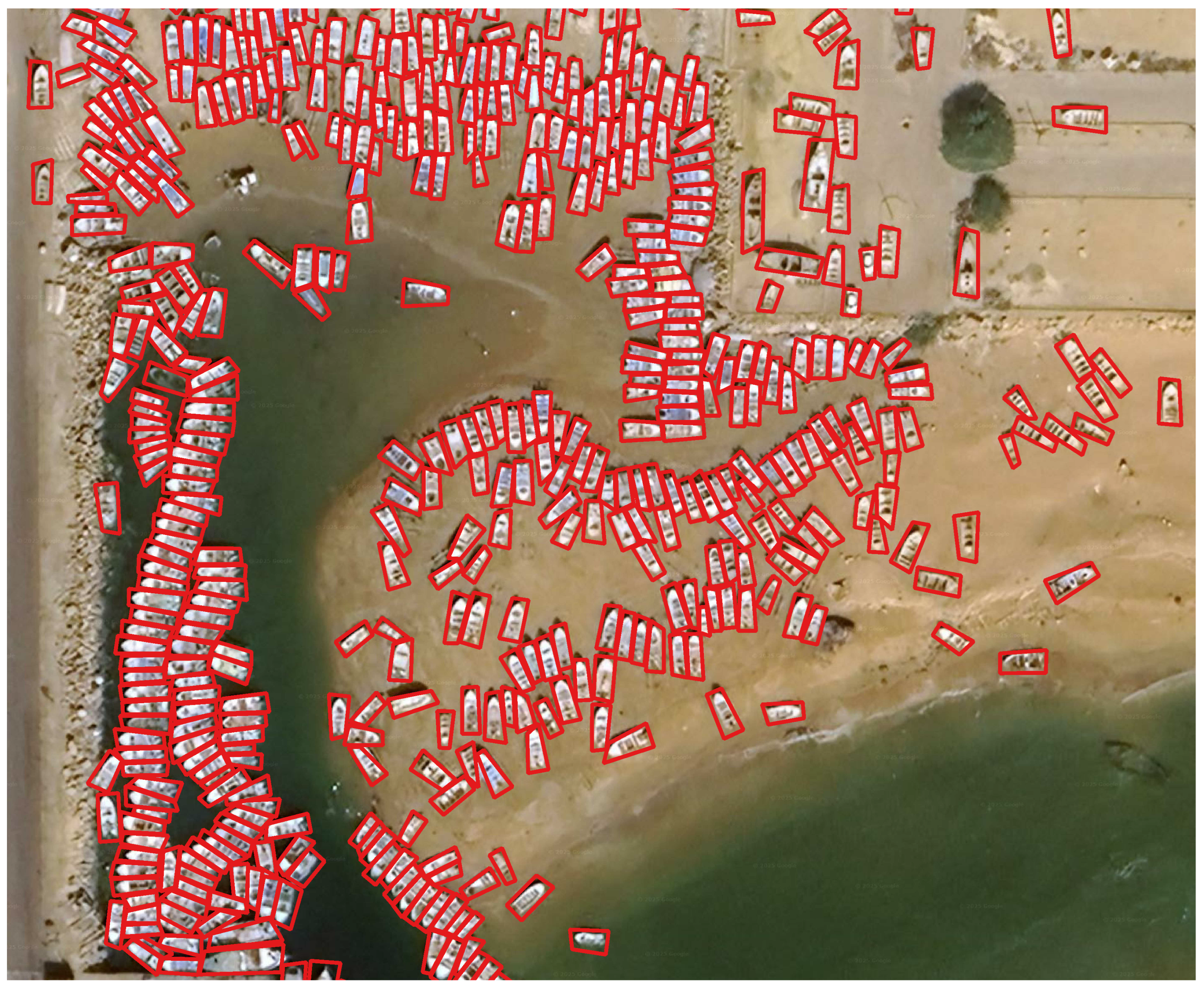
The dataset was manually annotated in QGIS (version 3.34) software by four expert annotators (the authors). Vessel boundaries were delineated using precise quadrilateral bounding boxes, with particular attention to difficult cases such as overlapping ships, low-contrast targets, and small maritime objects. The complete annotation process required approximately 100 person-hours. To ensure consistency and reliability, the annotators conducted regular calibration and cross-validation sessions. This rigorous procedure was essential for generating high-quality ground-truth labels suitable for training and evaluating segmentation models for small and overlapping vessels. In addition to bounding box coordinates, metadata such as vessel category, estimated length, and occlusion level were recorded. Figure 3 illustrates a sample image with their corresponding quadrilateral annotations.
It is worth noting that during dataset preparation, we also evaluated both SAM1 (Segment Anything Model version 1) [66] and SAM2 (Segment Anything Model version 2) [67] as potential tools for automatic or semi-automatic vessel mask generation. Although SAM demonstrates excellent generalization on natural scenes, its performance was limited in the maritime satellite domain. In particular, SAM frequently missed small vessels and often merged adjacent or overlapping ships into a single mask, and required considerable manual prompt refinement for low-contrast or wake-affected vessels. Consequently, SAM did not reduce the annotation workload for our dataset, and manual QGIS-based polygon annotation remained necessary to ensure accurate ground-truth segmentation.

3.1.2. Dataset Statistics

The resulting MAKSEA dataset contains 12,743 annotated vessel instances, with approximately 40% of scenes containing overlapping vessels—a factor that considerably increases detection and segmentation complexity. Vessel lengths range from under 10 m (small fishing boats and speedboats) to over 200 m (cargo ships and tankers). The dataset was partitioned into training (80%, 10,955 instances) and test (20%, 1788 instances) subsets using stratified sampling ensuring balanced category representation while maintaining geographic separation to avoid data leakage.
Compared with existing benchmarks, MAKSEA introduces unique challenges by emphasizing small, region-specific vessels, high inter-vessel density, and heterogeneous fleet compositions along a complex coastal region.

4. Materials and Methods

4.1. Architecture Overview

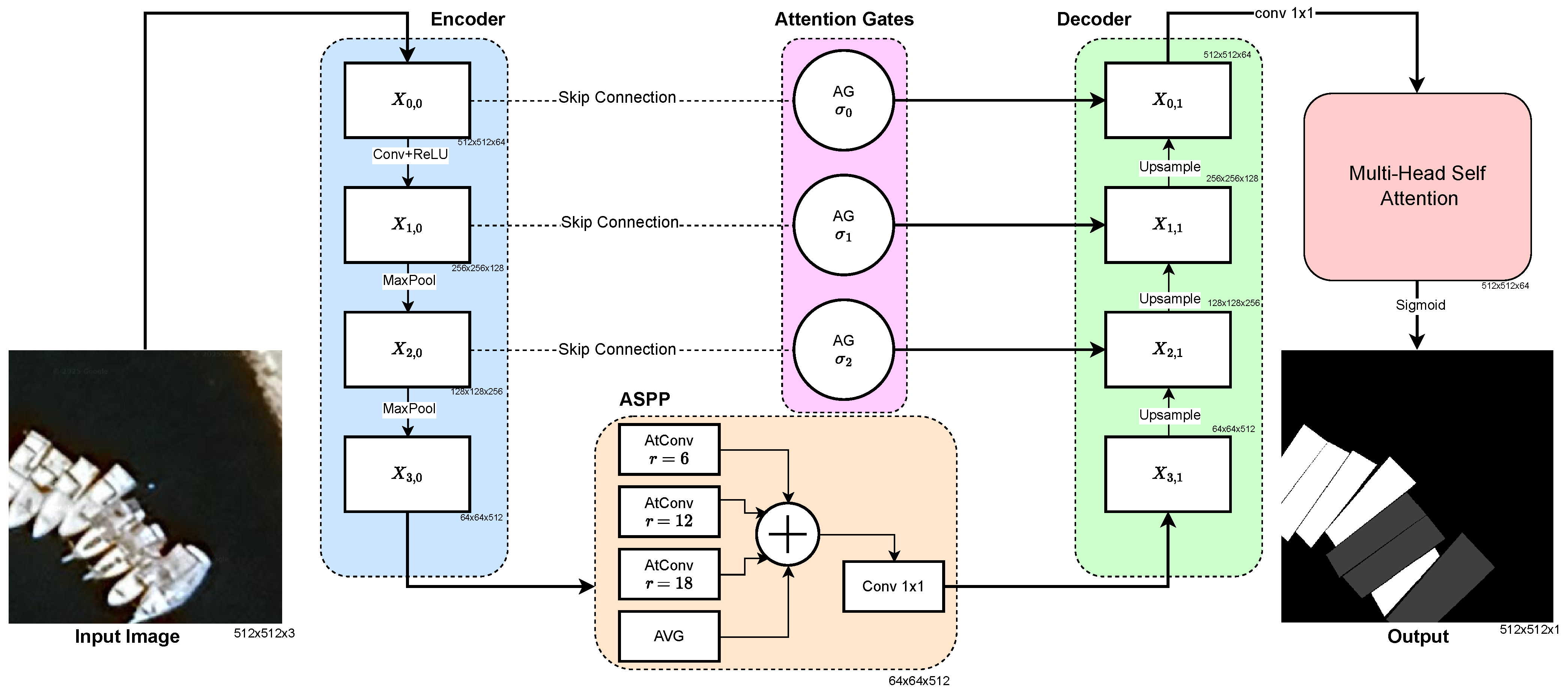
The proposed pipeline, MVSegNET, extends the U-Net++ framework [1] through strategic integration of ASPP and multi-scale attention mechanisms. While MVSegNet builds upon established architectural components—nested U-Net structures, ASPP modules, and attention mechanisms—that have proven effective across various domains including medical imaging [37,38,39], our contribution lies in their systematic optimization for the unique challenges of maritime vessel segmentation in satellite imagery. The core design philosophy addresses three critical challenges in maritime ship detection: multi-scale object variability, complex background interference, and precise boundary delineation. Figure 4 illustrates the overall architecture, where the input RGB image X R H × W × 3 undergoes hierarchical feature extraction through the encoder path, multi-scale context aggregation via ASPP, dense feature fusion through the decoder via attention-gated skip connections, and refined spatial representations through self-attention before generating the final segmentation mask.
Let X ( i , j ) denote the feature representation at encoder level i and decoder column j, where i { 0 , 1 , 2 , 3 } indexes the spatial resolution level and j { 0 , 1 , 2 , 3 } indexes the processing stage. The architecture maintains the dense connectivity pattern of U-Net++ while incorporating attention mechanisms at critical junctions to enhance feature selectivity and spatial coherence.

4.2. Enhanced U-Net++ Backbone with Dense Skip Connections

4.2.1. Dense Connectivity Formulation

The U-Net++ backbone employs nested dense skip pathways that aggregate features from multiple semantic levels. The output of each decoder node is formulated as:
X ( i , j ) = H ( X ( i , j 1 ) ) if j = 0 H X ( i , k ) k = 0 j 1 , U ( X ( i + 1 , j 1 ) ) if j > 0
where H ( · ) represents a sequence of 3 × 3 convolution, batch normalization, and ReLU activation operations, [ [ · ] ] denotes channel-wise concatenation, and U ( · ) represents bilinear upsampling followed by 1 × 1 convolution for channel alignment.

4.2.2. Feature Processing at Each Level

Each convolutional block H ( · ) consists of two consecutive operations:
H ( X ) = ReLU BN Conv 3 × 3 ReLU BN Conv 3 × 3 ( X )
where BN ( · ) denotes batch normalization and Conv 3 × 3 ( · ) represents 3 × 3 convolution with stride 1 and padding 1. The encoder employs max-pooling for downsampling with a factor of 2 at each level, progressively reducing spatial resolution from 512 2 to 32 2 while increasing channel dimensions from 64 to 512.

4.3. Atrous Spatial Pyramid Pooling (ASPP) Module

Since ships in satellite imagery vary significantly in size, ASPP is integrated at the bottleneck layer, enabling multi-scale context aggregation. ASPP applies atrous convolutions with different dilation rates r = [ 6 , 12 , 18 ] .

4.3.1. Multi-Scale Context Extraction

The ASPP module replaces the standard bottleneck layer to capture multi-scale contextual information important for detecting ships of varying sizes. Given the input feature map F R 32 × 32 × 512 from the encoder, ASPP applies parallel processing branches:
ASPP ( F ) = Concat [ B 1 ( F ) , B 2 ( F ) , B 3 ( F ) , B 4 ( F ) , B 5 ( F ) ]
where each branch B i processes features at different scales: B 1 ( F ) : 1 × 1 convolution for preserving fine details; B 2 ( F ) : 3 × 3 atrous convolution with dilation rate r = 6 ; B 3 ( F ) : 3 × 3 atrous convolution with dilation rate r = 12 ; B 4 ( F ) : 3 × 3 atrous convolution with dilation rate r = 18 ; and B 5 ( F ) : Global average pooling followed by 1 × 1 convolution.

4.3.2. Atrous Convolution Formulation

The atrous convolution operation for branch B i ( i { 2 , 3 , 4 } ) is defined as:
( F k r ) ( p ) = s + r · t = p F ( s ) · k ( t )
where k represents the 3 × 3 convolution kernel, r is the dilation rate, p denotes the output position, and ∗ denotes the convolution operation. The receptive field for rate r is calculated as:
RF = 1 + ( k 1 ) × r
yielding effective receptive fields of 7, 13, and 19 pixels for rates 6, 12, and 18, respectively.

4.3.3. Global Context Integration

The global branch B 5 ( F ) captures image-level contextual information:
B 5 ( F ) = Conv 1 × 1 Upsample Conv 1 × 1 GAP ( F )
where GAP ( · ) denotes global average pooling that computes the mean across all spatial locations:
GAP ( F ) c = 1 H × W i = 1 H j = 1 W F ( i , j , c )
The resulting features are processed through 1 × 1 convolutions and upsampled to match the spatial dimensions of other branches.

4.3.4. Feature Fusion and Output

All ASPP branches are concatenated and processed through a final fusion layer:
F ASPP = Conv 1 × 1 Concat B 1 , B 2 , B 3 , B 4 , B 5
which produces the enhanced feature representation F ASPP R 32 × 32 × 1024 that encodes multi-scale contextual information.

4.4. Attention Gate Mechanisms

To suppress irrelevant background clutter and emphasize ships, we use Attention Gates (AGs) on skip connections. Given encoder features x and decoder gating signal g, Attention gates are integrated at each skip connection to suppress irrelevant features and enhance ship specific information flow. For skip features F l R H × W × F l and gating signal g R H × W × F g from the decoder path, the attention mechanism computes:
q att l = ψ T σ 1 W x l F l + W g l F g + b g + b ψ
α l = σ 2 q att l
F ^ l = α l F l
where W x l R F l × F int and W g l R F g × F int are learned linear transformations. ψ R F int × 1 is the attention coefficient generator. F int = max ( F l , F g ) / 2 represents intermediate feature dimensions. σ 1 ( · ) and σ 2 ( · ) denote ReLU and sigmoid activation functions. ⊙ represents element-wise multiplication, and b g and b ψ are bias terms. The attention coefficient α l [ 0 , 1 ] H × W acts as a spatial attention map, where values close to 1 indicate ship relevant regions and values near 0 suppress background interference. The gate effectively learns to identify salient features based on the semantic information from higher-level decoder features.

4.5. Multi-Head Self-Attention Module

4.5.1. Self-Attention Mechanism

Inspired by [60], a multi-head self-attention module is incorporated after the final decoder layer X ( 0 , 3 ) to model long-range spatial dependencies that are crucial for maintaining ship-boundary coherence. Given input feature representations X R N × D where N = H × W is the flattened spatial dimension, the self-attention operation is defined as:
Attention ( Q , K , V ) = softmax Q K T d k V
where Q = X W Q , K = X W K , V = X W V   R N × d k are query, key, and value matrices derived from learned projections, with W Q , W K , W V R D × d k being trainable parameter matrices and d k = D / h representing the dimension per attention head.

4.5.2. Multi-Head Attention Formulation

The multi-head attention with h heads aggregates information from different representation subspaces:
MultiHead ( X ) = Concat ( head 1 , , head h ) W O
head i = Attention ( X W Q i , X W K i , X W V i )
where W Q i , W K i , W V i R D × d k are head-specific projection matrices and W O R h d k × D is the output projection matrix.

4.5.3. Positional Encoding Integration

To preserve spatial relationships, inspired by [60], we incorporate 2D sinusoidal positional encodings PE as follows:
PE ( p , 2 k ) = sin p 10000 2 k / D
PE ( p , 2 k + 1 ) = cos p 10000 2 k / D
where p denotes the 2D spatial position encoded as p = x + y × W , and k indexes the embedding dimension.

4.6. Loss Function Design

The final segmentation mask is produced through a 1 × 1 convolution followed by sigmoid activation ( σ ):
Y ^ = σ ( W o F + b o )
where F denotes the MHSA-refined decoder output. To address class imbalance and emphasize small-scale vessels, we adopt a Multi-Component Loss Formulation as follows:
L total = λ 1 L BCE + λ 2 L Dice + λ 3 L Focal + L DS
where λ 1 , λ 2 , λ 3 are balancing hyperparameters empirically set to 0.5, 0.3 and 0.2 respectively based on validation experiments. The L BCE denotes the Binary Cross-Entropy Loss and is defined as:
L BCE = 1 N i = 1 N [ y i log ( y ^ i ) + ( 1 y i ) log ( 1 y ^ i ) ]
where y i { 0 , 1 } denotes the label, N refers to the total number of pixels, and y ^ i [ 0 , 1 ] is the predicted output of the model. The Dice loss, L Dice , mitigates class imbalance by focusing on overlap between predicted and ground truth regions:
L Dice = 1 2 i = 1 N y i y ^ i + ϵ i = 1 N y i + i = 1 N y ^ i + ϵ
where ϵ = 1 × 10 7 is a smoothing term to prevent division by zero. The focal loss, L Focal , mitigates the impact of easy negatives and focuses learning on hard examples:
L Focal = 1 N i = 1 N α i ( 1 p i ) γ log ( p i )
where p i = y ^ i if y i = 1 else p i = 1 y ^ i , α i is the class weighting factor ( α 1 = 0.75 for ships, α 0 = 0.25 for background), and γ = 2 is the focusing parameter. Deep supervision loss, L DS , as defined below is applied at intermediate decoder outputs to enhance gradient propagation and stabilize network training:
L DS = l = 1 L w l · L seg ( Y l , Y ^ l )
where L = 3 supervision levels, w l = 1 / 2 L l are exponentially decreasing weights, Y l is the ground truth at level l, and Y ^ l is the corresponding prediction.

5. Experimental Results

5.1. Datasets

To comprehensively evaluate the performance and generalization capability of the proposed model, experiments were conducted on three benchmark datasets covering diverse imaging conditions and vessel categories. Specifically, we utilized two publicly available datasets—LEVIR_SHIP and DIOR_SHIP—along with our MAKSEA dataset whose details are provided in Section 3.

5.1.1. DIOR_SHIP Dataset

The DIOR_SHIP dataset, prepared in [70], is a subset of the large-scale Dataset for Object Recognition in Optical Remote Sensing (DIOR) [23]. It was specifically curated for ship instance segmentation in optical remote sensing imagery. The dataset comprises 1258 images with a spatial resolution of 800 × 800 pixels, covering diverse vessel sizes and orientations, with a predominance of small vessels. DIOR_SHIP provides a challenging benchmark due to significant scale variation and complex oceanic backgrounds. The key characteristics of this dataset are summarized in Table 1.

5.1.2. LEVIR_SHIP Dataset

The LEVIR_SHIP dataset, also introduced in [70], is derived from the Large-Scale VHR Optical Remote Sensing Vehicle Detection (LEVIR) dataset [22]. Whereas the original LEVIR dataset focuses on vehicles such as cars and trucks, LEVIR_SHIP was re-annotated for ship instance segmentation tasks. It contains 1461 annotated ship instances, of which 1222 are small vessels, making it particularly suitable for assessing methods that focus on small and densely distributed maritime objects. The detailed statistics of this dataset are summarized in Table 1.

5.1.3. MAKSEA Dataset

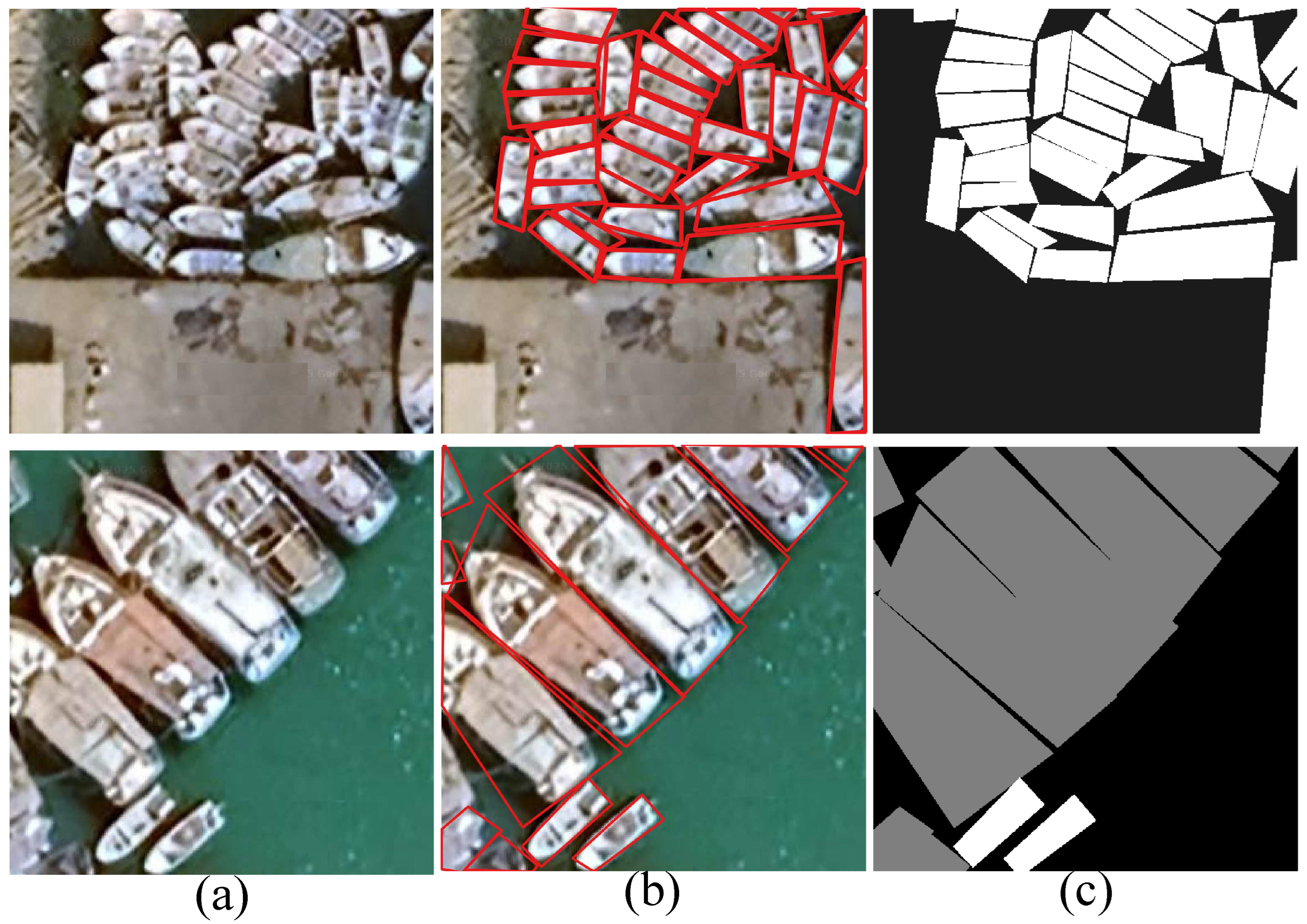
As described in Section 3, the prepared MAKSEA dataset comprises 20 high-resolution satellite images acquired from the Makkoran coast. Unlike conventional benchmark datasets that rely on rectangular bounding boxes, we utilize QGIS to annotate each image with quadrilateral bounding boxes, represented as [ x 1 , y 1 , x 2 , y 2 , x 3 , y 3 , x 4 , y 4 ] , enabling more precise characterization of vessel geometry and orientation—particularly for overlapping and densely clustered instances. All images are subsequently resized to a resolution of 512 × 512 pixels (Figure 5a). In total, MAKSEA contains 12,473 annotated and resized images, whose quadrilateral annotations (Figure 5b) are converted into pixel-level segmentation masks used for model training and evaluation (Figure 5c). Table 1 summarizes key statistics of the MAKSEA dataset in comparison with other benchmark datasets.
It is worth mentioning that, similar to many remote sensing datasets, our segmentation masks are derived from quadrilateral bounding box (QBB) annotations, resulting in quadrilateral approximations rather than pixel-accurate vessel contours. This choice reflects the practical constraints of large-scale dataset creation, where precise polygon tracing is prohibitively time-consuming. While these masks do not capture fine hull curvature, they provide sufficient accuracy for operational maritime applications such as localization, heading estimation, and traffic monitoring, and remain consistent with common annotation practices in geospatial analysis.
Since the original ground-truth annotations were generated using quadrilateral bounding boxes, while the evaluated models produce segmentation-based outputs, we applied an output-vector regularization procedure during evaluation, following the methodology outlined in [71]. This regularization ensures consistency between the geometric annotation format and the segmentation-derived predictions. A comparative illustration between the raw output vectors and their regularized counterparts is provided in Figure 6.

5.2. Evaluation Metrics

Model performance is assessed using well-known evaluation metrics that quantify distinct aspects of segmentation quality. The mathematical formulations for each metric are presented below to ensure reproducibility and clarity. The Intersection over Union (IoU), measures the overlap between predicted and ground truth regions of the given input image.
IoU = T P T P + F P + F N
where TP is true positives, FP is false positives, and FN is false negatives. We also evaluate the models using the Dice coefficient as follows that measure the balance between precision and recall metrics (25):
Dice = 2 × T P 2 × T P + F P + F N
Precision reflect the accuracy of positive predictions, while recall measure the completeness of the detections and can be defines as follows, and Accuracy measures the overall proportion of correctly classified pixels (both foreground and background) relative to all pixels in the image. These metrics are computed as follows:
Precision = T P T P + F P , Recall = T P T P + F N , Accuracy = T P + T N T P + T N + F P + F N
Average precision (AP) summarizes the precision-recall curve across different confidence thresholds:
AP = 0 1 P ( R ) d R
where P ( R ) represents precision as a function of recall. For multi-class scenarios, Mean Average Precision (mAP) computes the mean AP across all classes:
mAP = 1 C c = 1 C AP c
where C is the number of classes and AP c is the average precision for class c, where c = 1 in our proposed model.
In maritime surveillance, missing a vessel (false negative) is generally more important than over-segmenting a vessel (false positive), especially for security, illegal fishing detection, and maritime traffic monitoring. However, because segmentation masks are required for downstream tasks (e.g., vessel sizing, area estimation), both precision and recall matter. While IoU is still the most appropriate global metric for segmentation quality, Recall is slightly more important operationally.

5.3. Implementation Details

The proposed framework and the baseline models are implemented and inferenced on a single NVIDIA RTX 4090 GPU with 24 GB of memory. The Atrous Spatial Pyramid Pooling (ASPP) module consisted of four parallel branches with dilation rates of 6, 12, and 18, in addition to a 1 × 1 convolution and a global average pooling branch. Each branch produced 256 feature maps, which are concatenated into 1280 channels and subsequently reduced to 512 via a 1 × 1 convolution. The multi-head self-attention (MHSA) module employed eight heads with a head dimension of 64, resulting in a total embedding size of 512. Two-dimensional sinusoidal positional encodings are applied with distinct horizontal and vertical frequencies. Attention gates are designed with intermediate channel dimensions equal to half the maximum of the input and gating signal sizes. Deep supervision are applied at three decoder stages with exponentially decaying weights of 0.5, 0.25, and 0.125, respectively. The network are trained using a hybrid loss function (18).
Training are conducted using the AdamW optimizer [72] with an initial learning rate of 1 × 10 4 and a weight decay of 0.1 for 100 epochs. A cosine annealing schedule with warm restarts gradually reduced the learning rate to 1 × 10 6 over 50 epochs. The batch size was set to 16 per GPU, with gradient accumulation over two steps for an effective batch size of 32. To improve model generalization, data augmentation techniques included random flips ( p f = 0.5 ), rotations within ± 15 ° , and brightness/contrast adjustments within δ b c = ± 0.2 .

5.4. Quantitative and Qualitative Comparison Against SoTA Methods

5.4.1. DIOR_SHIP Benchmark Dataset

Table 2 illustrates the quantitative results of the proposed model with state-of-the-art approaches on DIOR_SHIP dataset [23]. As shown, our model outperformed the SoTA models with ∼4% margin in almost all the evaluation metrics used for measurements. The only method achieving better performance is Trans-UNet [62] that performed better (0.9903) than our model (0.9542) in terms of Accuracy.
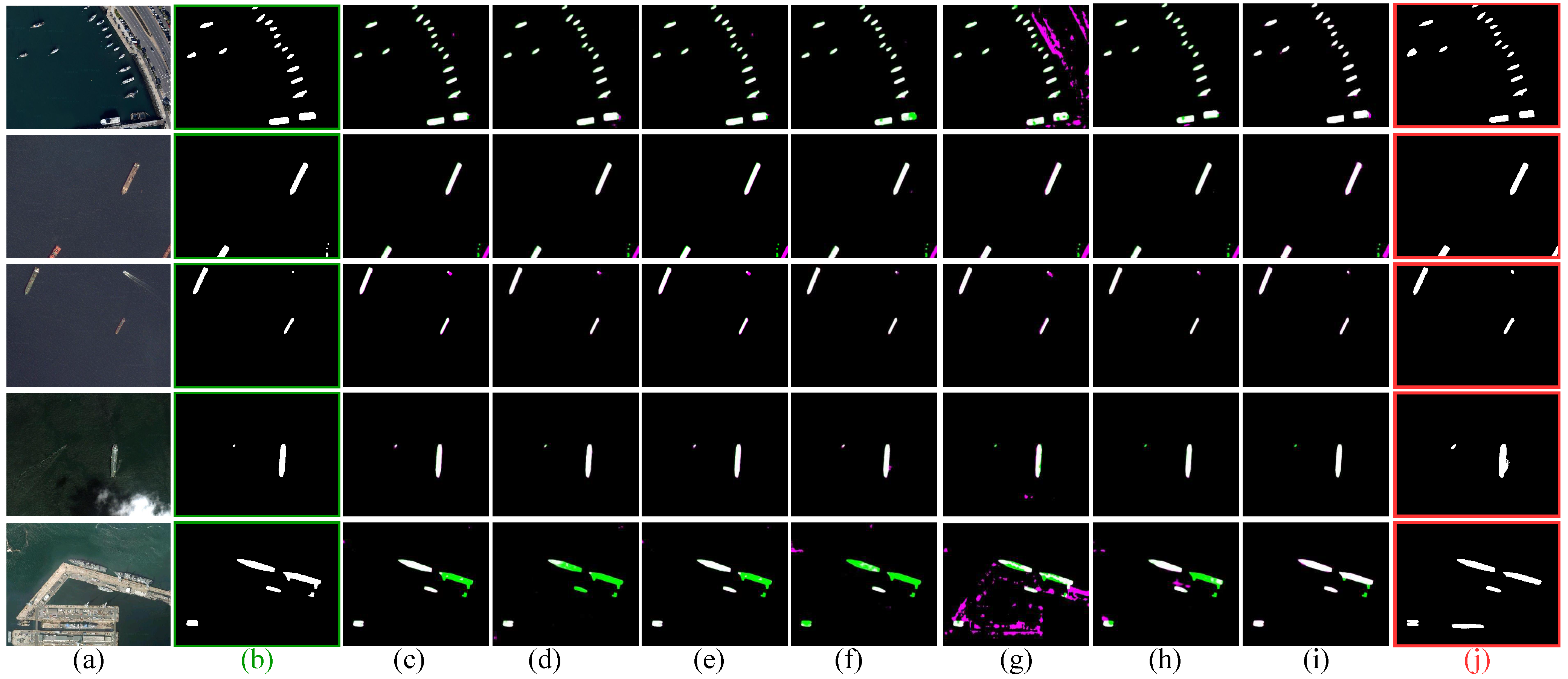
To evaluate the effect of our model on real-world scenes, we compared it on challenging sample images of the DIOR_SHIP dataset in Figure 7. The results in Figure 7j validate the quantitative performance in Table 2.

5.4.2. LEVIR_SHIP Benchmark Dataset

We also compare our model with the SoTA architectures [26,32,33,34,35,62,70] on the LEVIR_SHIP [22] benchmark. As shown in Table 3, our model also achieved superior performance across most evaluation metrics.
The visual comparison of our model with other segmentation methods on challenging examples from the LEVIR_SHIP benchmark, as shown in Figure 8, also confirm that our model segments small and adjacent ship instances more accurately.

5.4.3. Comparison of SoTA Models on MAKSEA Dataset

Table 4 presents a comprehensive quantitative comparison between the proposed method and existing SoTA segmentation approaches on the MAKSEA dataset. Our method achieves superior performance across all evaluation metrics, demonstrating its effectiveness for ship segmentation SAR images with small and overlapped ship instances. MVSegNet also outperforms a recent model, SCUNet++ [40], on maritime vessel segmentation tasks. This superior performance is attributed to our domain-specific architectural adaptations that address the unique challenges of satellite-based maritime vessel detection: extreme scale variations, severe overlapping in crowded ports, and low vessel-water contrast.
Our proposed method achieves an IoU of 0.826, representing a 12.3% relative improvement over the baseline U-Net and a 7.0% improvement over the standard U-Net++. Similarly, the Dice coefficient reaches 0.885, indicating a higher degree of overlap between predicted and ground truth regions. The precision and recall values of 0.879 and 0.881, respectively, demonstrate balanced performance with trade-off between detection accuracy and completeness. The average precision of 0.857 and false positive rate of 0.062 further confirm the method’s robustness in distinguishing ships from complex oceanic backgrounds.
While quantitative metrics provide global performance trends, they may not fully reflect the challenges posed by the difficulty of overlapping small vessels, which is a critical aspect of the MAKSEA dataset. To address this limitation, a qualitative visual analysis is conducted by comparing predicted outputs against ground-truth annotations in densely clustered harbor scenes. Figure 9 demonstrates the qualitative comparisons of our model among SoTA models on challenging images of the MAKSEA dataset including isolated ships, dense ship clusters, and small overlapped ship instances. As seen, the qualitative results highlight several distinctive advantages of our approach compared with the U-Net and U-Net++ that often struggled to delineate boundaries in crowded harbors, producing merged masks for adjacent vessels.
Although quadrilateral mask labels were used for training of our model, the qualitative results in Figure 9 demonstrate that MVSegNet is capable of producing segmentation masks that more closely follow the true geometric structure of the vessels. For isolated ships, our method produces cleaner boundaries with fewer artifacts compared to the baseline U-Net++. In dense ship clusters, the self-attention mechanism effectively separates adjacent vessels that are often merged by other methods. Under challenging conditions such as low-resolution, crowded ship instances, the attention gates successfully suppress false positives while maintaining high detection sensitivity. The proposed method demonstrates strong performance in segmenting small ships, where the combination of multi-scale processing and attention mechanisms enables the identification of vessels often missed by baseline approaches.

5.5. Ablation Experiments

5.5.1. Effect of the Utilized Components on the Proposed Model

To evaluate the effectiveness of each module within the proposed architecture, we perform comprehensive ablation experiments to quantify the contribution of individual components on the MAKSEA dataset. The baseline configuration corresponds to the standard U-Net++ model without any of the proposed enhancements, serving as the reference for all subsequent comparisons.
As illustrated in Table 5, the ablation results demonstrate the incremental benefits of each component. The ASPP module provides the most significant improvement, increasing IoU from 0.756 to 0.793 (4.9% absolute improvement) by effectively capturing multi-scale contextual information. We also evaluated different ASPP configurations to determine the optimal dilation rate combination. The configuration with dilation rates [6, 12, 18] achieved the best balance between receptive field coverage and feature resolution, providing optimal performance for ship detection. Including a fourth dilation rate (24) yielded minimal additional benefit while increasing computational complexity.
Attention gates further enhance performance to 0.812 IoU by selectively emphasizing ship relevant features and suppressing background interference. The self-attention module contributes an additional improvement, bringing the final IoU to 0.826 through better modeling of long-range spatial dependencies for improved boundary coherence. To further assess the individual contributions of different attention mechanisms, we conducted experiments with multiple attention-configuration variants. Table 6 summarizes the performance results obtained for each attention-mechanism combination.
The results show that both attention mechanisms contribute substantially to overall performance, with the attention gates yielding a slightly greater improvement than the self-attention module when applied individually. Nonetheless, the combined configuration produces the best results, highlighting the complementary nature of the two mechanisms in addressing distinct aspects of the ship-segmentation problem, namely local feature emphasis and global contextual modeling.

5.5.2. Ablation Study on Vessel Size and Geodetic Area Analysis

To assess the robustness of MVSegNet across different vessel scales, we conducted an ablation experiment based on the geodetic areas of annotated ships in the MAKSEA dataset. Since the original imagery was obtained from Google Earth and manually labeled in QGIS, the true surface area of each vessel could be computed directly from its polygonal annotation. All area calculations were performed on the WGS 84 ellipsoid (EPSG:7030), ensuring geodetically accurate measurements that avoid the distortions inherent in planar Cartesian approximations. This ellipsoidal approach provides reliable and consistent area estimates suitable for maritime monitoring applications.
Ships were grouped into three size categories according to their geodetic area: small (≤ 20 m 2 ), medium (20– 200 m 2 ), and large (≥ 200 m 2 ). Table 7 presents the segmentation performance of MVSegNet for each category, highlighting the model’s stability across scales and the expected challenge associated with detecting very small vessels.
The results demonstrate consistent performance across all ship-size categories, with particularly strong outcomes for small vessels (IoU = 0.781), which represent the most challenging class for accurate segmentation. The ASPP module, through its multi-scale processing capability, effectively mitigates the scale-variation problem. Meanwhile, the attention mechanisms help maintain detection accuracy for small objects by suppressing background interference and enhancing feature discrimination.

5.5.3. Cross-Dataset Generalization

To evaluate the generalization capability of the proposed model, cross-dataset experiments were conducted by training and testing on different combinations of the prepared MAKSEA dataset and two benchmark datasets, DIOR_SHIP and LEVIR_SHIP.
Table 8 summarizes the results, revealing the model’s robustness across diverse imaging modalities and environmental conditions. As shown in Table 8, when the model was trained on DIOR_SHIP or LEVIR_SHIP and evaluated on MAKSEA, a noticeable decrease in segmentation accuracy was observed, with IoU values of 0.698 and 0.712, respectively. This degradation indicates that MAKSEA poses a greater challenge, likely due to its more complex environmental variations, imaging angles, and inclusion of both optical and SAR modalities.
In contrast, when trained on MAKSEA and tested on the benchmark datasets, the model achieved significantly higher performance (IoU > 0.789 and Dice > 0.841), surpassing the reverse settings by a large margin. This asymmetric generalization pattern suggests that features learned from MAKSEA are more discriminative and transferable, effectively capturing domain-invariant characteristics such as vessel geometry and context under varying illumination and backgrounds.
Overall, these findings demonstrate that training on the proposed MAKSEA dataset enhances the model’s ability to generalize across different imaging domains and geographic distributions, underscoring the dataset’s richness and the robustness of the proposed approach against domain shifts.

5.5.4. Computational Efficiency

We also conducted further experiments to evaluate the computational efficiency of the proposed MVSegNET against SoTA standard segmentation baselines (Table 9). As shown, our model demonstrates superior parameter efficiency, requiring only 24.7 million parameters—approximately 2.7× fewer than standard U-Net (66.8 M) and 3.2× fewer than UNet++ (79.4 M). More critically for practical deployment, the proposed architecture processes batches of sixteen 512 × 512 images in 65 ms on an RTX 4090 GPU, outperforming UNet++ (136.2 ms) by 2.1× and TransUNet (182.3 ms) by 2.8×. At 65.4 ms per 512 × 512 tile, MVSegNet operates at 15.3 FPS (Frame-Per-Second), which is adequate for near-real-time maritime monitoring, similar or faster than SoTA models under comparison. This efficiency stems from our effective integration of ASPP and attention mechanisms, which replaces the heavy bottleneck of traditional U-Net architectures while maintaining multi-scale receptive fields.

5.6. Discussion

5.6.1. Interpretation of Results

The experimental results indicate that the proposed architecture substantially outperforms existing segmentation methods across multiple benchmarks. Specifically, it achieves a 12.3% improvement in IoU over U-Net and a 7.0% gain over U-Net++, validating the effectiveness of its integrated modules in addressing ship detection challenges in satellite imagery. The ASPP module enhances multi-scale context modeling, improving the detection of small vessels that conventional networks often overlook. By capturing contextual cues across diverse receptive fields, the model effectively recognizes vessels at varying scales without requiring distinct processing pathways. Attention mechanisms also play a critical role in mitigating false positives by emphasizing ship-relevant features while suppressing background noise. The 18.7% reduction in false positive rate relative to the baseline highlights this benefit, especially in complex maritime scenes with complex wave textures. Furthermore, the self-attention component improves boundary coherence, particularly in dense harbor scenes where ships appear in close proximity. The 8.9% increase in boundary accuracy underscores the advantage of modeling long-range spatial dependencies for precise instance delineation.

5.6.2. Limitations and Future Work

Despite our model’s overall robustness and SoTA results, our model fails in challenging scenarios. The model’s performance on extremely small vessels (≤10 m2) is still limited, indicating the need for specialized small-object enhancement strategies. Typical failure cases include severe occlusion, irregular vessel shapes, and adverse weather conditions. These cases suggest potential improvements through enhanced occlusion modeling and the inclusion of more diverse training samples covering rare ship types and environmental variations.
Although MVSegNet focuses on binary ship segmentation, it does not explicitly perform ship-size classification. However, size categories can be inferred in a post-processing step by computing the area of each segmented vessel and mapping it to predefined size thresholds. Future work will integrate this capability directly into the network by extending MVSegNet with a multi-task prediction head that jointly performs segmentation and size-category classification. Such an end-to-end technique would enable richer maritime analytics and reduce reliance on external post-processing steps.
In Future work, we will explore multi-resolution processing pipelines to better manage scale variability and temporal modeling to leverage motion cues from image sequences. Additionally, domain adaptation techniques could improve generalization across different sensors and imaging conditions, minimizing retraining requirements. Extending the framework toward multi-class ship detection and classification would further enhance maritime situational awareness by distinguishing vessel categories such as cargo, fishing, and military ships.

6. Conclusions

In this paper, we present MVSegNet, a deep learning framework for accurate segmentation of small and densely distributed vessels in satellite images. The model uses three main modules: an Atrous Spatial Pyramid Pooling (ASPP) block to capture vessels at different scales, attention-guided skip connections to reduce ocean background noise, and a self-attention block to model long-range spatial relationships. We also introduced MAKSEA, a new dataset collected from the Makkoran coast, which contains small, overlapping, and densely packed vessels under complex maritime conditions. Experiments on the MAKSEA, LEVIR_SHIP, and DIOR_SHIP datasets show that MVSegNet achieves high performances in terms of several evaluation metrics, and outperforms several SoTA models. The proposed model obtained an IoU of 0.826 on MAKSEA and F1-scores of 0.9028 and 0.9607 on LEVIR_SHIP and DIOR_SHIP, respectively.

Author Contributions

Z.R. conceived the study, implemented the methodology, wrote the original manuscript, and contributed to data annotation. V.N.H. contributed to the manuscript revision and data annotation, and was involved in conducting the ablation experiments. R.D. performed data annotation, revised the manuscript, and conduced some parts of the model experiments. E.S. collected the dataset, revised the manuscript, and contributed to data annotation and experiments. All authors have read and agreed to the published version of the manuscript.

Funding

This research received no external funding.

Data Availability Statement

The DIOR_SHIP and LEVIR_SHIP dataset can be downloaded from https://github.com/wzp8023391/Ship_Segmentation (accessed on 1 November 2025), and our presented MAKSEA dataset is available at https://github.com/zobeirraisi/MAKSEA (accessed on 15 December 2025). The code of this work will be released at the mentioned repository after acceptance of the manuscript.

Acknowledgments

The authors gratefully acknowledge the support provided by Makkoran Vision AI Company throughout this research. Their technical expertise in artificial intelligence and computer vision, along with the resources they generously provided, were essential to the success of this project.

Conflicts of Interest

The authors declare no conflicts of interest.

Abbreviations

The following abbreviations are used in this manuscript:
MVSegNetMakkoran Vessel Segmentation Network
SoTAState of The Art
IoUIntersection over Union
ASPPAtrous Spatial Pyramid Pooling
CNNsConvolutional Neural Networks

References

  1. Kanjir, U.; Greidanus, H.; Štir, K. Vehicle Detection in Very High Resolution Satellite Images of City Areas. IEEE Trans. Geosci. Remote Sens. 2018, 56, 2311–2323. [Google Scholar]
  2. Corbane, C.; Carrion, D.; Lemoine, G.; Broglia, M. Rapid Damage Assessment Using High Resolution Satellite Imagery and Semi-Automatic Object-Based Image Analysis: The Case of the 2003 Bam Earthquake. Photogramm. Eng. Remote Sens. 2008, 74, 1021–1035. [Google Scholar]
  3. Patel, K.; Bhatt, C.; Mazzeo, P.L. Deep Learning-Based Automatic Detection of Ships: An Experimental Study Using Satellite Images. J. Imaging 2022, 8, 182. [Google Scholar] [CrossRef]
  4. Reggiannini, M.; Salerno, E.; Bacciu, C.; D’Errico, A.; Lo Duca, A.; Marchetti, A.; Martinelli, M.; Mercurio, C.; Mistretta, A.; Righi, M.; et al. Remote Sensing for Maritime Traffic Understanding. Remote Sens. 2024, 16, 557. [Google Scholar] [CrossRef]
  5. Li, H.; Wang, D.; Hu, J.; Zhi, X.; Yang, D. FANT-Det: Flow-Aligned Nested Transformer for SAR Small Ship Detection. Remote Sens. 2025, 17, 3416. [Google Scholar] [CrossRef]
  6. Zhao, T.; Wang, Y.; Li, Z.; Gao, Y.; Chen, C.; Feng, H.; Zhao, Z. Ship Detection with Deep Learning in Optical Remote-Sensing Images: A Survey of Challenges and Advances. Remote Sens. 2024, 16, 1145. [Google Scholar] [CrossRef]
  7. Wang, L.; Zhou, Z.; Luo, R.; Zhao, L.; Liu, L. Small Ship Detection in SAR Images Based on Asymmetric Feature Learning and Shallow Context Embedding. IEEE J. Sel. Top. Appl. Earth Obs. Remote Sens. 2025, 18, 28466–28479. [Google Scholar] [CrossRef]
  8. Corbane, C.; Najman, L.; Pecoul, E.; Demagistri, L.; Petit, M. A Complete Processing Chain for Ship Detection Using Optical Satellite Imagery. Int. J. Remote Sens. 2010, 31, 5837–5854. [Google Scholar] [CrossRef]
  9. Leng, X.; Ji, K.; Yang, K.; Zou, H. Ship Detection Based on Fusion of Multi-Feature and Sparse Representation in High-Resolution SAR Images. J. Syst. Eng. Electron. 2015, 26, 736–743. [Google Scholar]
  10. Dalal, N.; Triggs, B. Histograms of Oriented Gradients for Human Detection. In Proceedings of the 2005 IEEE Computer Society Conference on Computer Vision and Pattern Recognition (CVPR’05), San Diego, CA, USA, 20–25 June 2005; Volume 1, pp. 886–893. [Google Scholar]
  11. Lowe, D.G. Distinctive Image Features from Scale-Invariant Keypoints. Int. J. Comput. Vis. 2004, 60, 91–110. [Google Scholar] [CrossRef]
  12. Cortes, C.; Vapnik, V. Support-Vector Networks. Mach. Learn. 1995, 20, 273–297. [Google Scholar] [CrossRef]
  13. Yasir, M.; Jianhua, W.; Mingming, X.; Hui, S.; Zhe, Z.; Shanwei, L.; Colak, A.T.I.; Hossain, M.S. Ship Detection Based on Deep Learning Using SAR Imagery: A Systematic Literature Review. Soft Comput. 2023, 27, 63–84. [Google Scholar] [CrossRef]
  14. Cheng, G.; Han, J.; Zhou, P.; Guo, L. Multi-Feature Fusion for Ship Detection in Optical Satellite Images. IEEE Trans. Geosci. Remote Sens. 2014, 52, 4992–5004. [Google Scholar]
  15. Schmidhuber, J. Deep Learning in Neural Networks: An Overview. Neural Netw. 2015, 61, 85–117. [Google Scholar] [CrossRef]
  16. LeCun, Y.; Bengio, Y.; Hinton, G. Deep Learning. Nature 2015, 521, 436–444. [Google Scholar] [CrossRef] [PubMed]
  17. Zhang, R.; Yao, J.; Zhang, K.; Feng, C.; Zhang, J. A Deep Learning Approach for Ship Detection from Satellite Imagery. ISPRS Int. J. Geo-Inf. 2016, 5, 142. [Google Scholar]
  18. He, K.; Zhang, X.; Ren, S.; Sun, J. Deep Residual Learning for Image Recognition. In Proceedings of the IEEE Conference on Computer Vision and Pattern Recognition, Las Vegas, NV, USA, 27–30 June 2016; pp. 770–778. [Google Scholar]
  19. Redmon, J.; Farhadi, A. YOLOv3: An Incremental Improvement. arXiv 2018, arXiv:1804.02767. [Google Scholar] [CrossRef]
  20. Liu, Z.; Hu, J.; Weng, L.; Yang, Y. HRSC2016: A High-Resolution Ship Collection for Ship Detection in Optical Remote Sensing Images. In Proceedings of the 2017 IEEE International Geoscience and Remote Sensing Symposium (IGARSS), Fort Worth, TX, USA, 23–28 July 2017; pp. 620–623. [Google Scholar]
  21. Airbus, A. Airbus Ship Detection Challenge. 2018. Available online: https://www.kaggle.com/c/airbus-ship-detection (accessed on 1 November 2025).
  22. Zou, Z.; Shi, Z. Random Access Memories: A New Paradigm for Target Detection in High Resolution Aerial Remote Sensing Images. IEEE Trans. Image Process. 2018, 27, 1100–1111. [Google Scholar] [CrossRef]
  23. Li, K.; Wan, G.; Cheng, G.; Meng, L.; Han, J. Object Detection in Optical Remote Sensing Images: A Survey and a New Benchmark. ISPRS J. Photogramm. Remote Sens. 2020, 159, 296–307. [Google Scholar] [CrossRef]
  24. Redmon, J.; Divvala, S.; Girshick, R.; Farhadi, A. You Only Look Once: Unified, Real-Time Object Detection. In Proceedings of the IEEE Conference on Computer Vision and Pattern Recognition, Las Vegas, NV, USA, 27–30 June 2016; pp. 779–788. [Google Scholar]
  25. Ren, S.; He, K.; Girshick, R.; Sun, J. Faster R-CNN: Towards Real-Time Object Detection with Region Proposal Networks. In Proceedings of the Advances in Neural Information Processing Systems, Montreal, QC, Canada, 7–12 December 2015; pp. 91–99. [Google Scholar]
  26. Ronneberger, O.; Fischer, P.; Brox, T. U-Net: Convolutional Networks for Biomedical Image Segmentation. In Proceedings of the International Conference on Medical Image Computing and Computer-Assisted Intervention, Munich, Germany, 5–9 October 2015; pp. 234–241. [Google Scholar]
  27. Girshick, R. Fast R-CNN. In Proceedings of the IEEE International Conference on Computer Vision, Santiago, Chile, 7–13 December 2015; pp. 1440–1448. [Google Scholar]
  28. He, K.; Zhang, X.; Ren, S.; Sun, J. Spatial Pyramid Pooling in Deep Convolutional Networks for Visual Recognition. In Proceedings of the European Conference on Computer Vision, Zurich, Switzerland, 6–12 September 2014; pp. 346–361. [Google Scholar]
  29. Liu, W.; Anguelov, D.; Erhan, D.; Szegedy, C.; Reed, S.; Fu, C.-Y.; Berg, A.C. SSD: Single Shot MultiBox Detector. In Proceedings of the European Conference on Computer Vision, Amsterdam, The Netherlands, 11–14 October 2016; pp. 21–37. [Google Scholar]
  30. Long, J.; Shelhamer, E.; Darrell, T. Fully Convolutional Networks for Semantic Segmentation. In Proceedings of the IEEE Conference on Computer Vision and Pattern Recognition (CVPR), Boston, MA, USA, 7–12 June 2015; pp. 3431–3440. [Google Scholar]
  31. He, K.; Gkioxari, G.; Dollár, P.; Girshick, R. Mask R-CNN. In Proceedings of the IEEE International Conference on Computer Vision (ICCV), Venice, Italy, 22–29 October 2017; pp. 2961–2969. [Google Scholar]
  32. Zhou, Z.; Rahman Siddiquee, M.M.; Tajbakhsh, N.; Liang, J. UNet++: A Nested U-Net Architecture for Medical Image Segmentation. IEEE Trans. Med. Imaging 2018, 39, 1856–1867. [Google Scholar] [CrossRef] [PubMed]
  33. Badrinarayanan, V.; Kendall, A.; Cipolla, R. SegNet: A Deep Convolutional Encoder-Decoder Architecture for Image Segmentation. IEEE Trans. Pattern Anal. Mach. Intell. 2017, 39, 2481–2495. [Google Scholar] [CrossRef]
  34. Chen, L.-C.; Zhu, Y.; Papandreou, G.; Schroff, F.; Adam, H. Encoder-Decoder with Atrous Separable Convolution for Semantic Image Segmentation. In Proceedings of the European Conference on Computer Vision (ECCV), Munich, Germany, 8–14 September 2018; pp. 801–818. [Google Scholar]
  35. Xie, E.; Wang, W.; Yu, Z.; Anandkumar, A.; Alvarez, J.M.; Luo, P. SegFormer: Simple and Efficient Design for Semantic Segmentation with Transformers. In Proceedings of the Advances in Neural Information Processing Systems (NeurIPS), Virtual, 6–14 December 2021. [Google Scholar]
  36. Gao, G.; Xu, G.; Yu, Y.; Xie, J.; Yang, J.; Yue, D. MSCFNet: A lightweight network with multi-scale context fusion for real-time semantic segmentation. IEEE Trans. Intell. Transp. Syst. 2021, 23, 25489–25499. [Google Scholar] [CrossRef]
  37. Liu, K.; Xie, J.; Chen, M.; Chen, H.; Liu, W. MA-UNet++: A multi-attention guided U-Net++ for COVID-19 CT segmentation. In Proceedings of the 2022 13th Asian Control Conference (ASCC), Jeju, Republic of Korea, 4–7 May 2022; pp. 682–687. [Google Scholar]
  38. Niyogisubizo, J.; Zhao, K.; Meng, J.; Pan, Y.; Didi, R.; Wei, Y. Attention-guided residual U-Net with SE connection and ASPP for watershed-based cell segmentation in microscopy images. J. Comput. Biol. 2025, 32, 225–237. [Google Scholar] [CrossRef]
  39. Zhang, H.; Zhu, C.; Lian, X.; Hua, F. A nested attention guided UNet++ architecture for white matter hyperintensity segmentation. IEEE Access 2023, 11, 66910–66920. [Google Scholar] [CrossRef]
  40. Chen, Y.; Zou, B.; Guo, Z.; Huang, Y.; Huang, Y.; Qin, F.; Li, Q.; Wang, C. SCUNet++: Swin-UNet and CNN bottleneck hybrid architecture with multi-fusion dense skip connection for pulmonary embolism CT image segmentation. In Proceedings of the IEEE/CVF Winter Conference on Applications of Computer Vision (WACV), Waikoloa, HI, USA, 3–8 January 2024; pp. 7759–7767. [Google Scholar]
  41. Liu, N.; Lu, Z.; Lian, W.; Tian, M.; Ma, C.; Peng, L. HMSAM-UNet: A hierarchical multi-scale attention module-based convolutional neural network for improved CT image segmentation. IEEE Access 2024, 12, 79415–79427. [Google Scholar] [CrossRef]
  42. Bui, L.; Phung, S.L.; Di, Y.; Le, H.T.; Nguyen, T.T.P.; Burden, S.; Bouzerdoum, A. UOW-Vessel: A Benchmark Dataset of High-Resolution Optical Satellite Images for Vessel Detection and Segmentation. In Proceedings of the IEEE/CVF Workshop on Applications of Computer Vision (WACV), Waikoloa, HI, USA, 3–7 January 2024; pp. 4416–4424. [Google Scholar]
  43. Xia, G.-S.; Bai, X.; Ding, J.; Zhu, Z.; Belongie, S.J.; Luo, J.; Datcu, M.; Pelillo, M.; Zhang, L. DOTA: A Large-Scale Dataset for Object Detection in Aerial Images. In Proceedings of the IEEE/CVF Conference on Computer Vision and Pattern Recognition (CVPR), Salt Lake City, UT, USA, 18–23 June 2018. [Google Scholar]
  44. Bovolo, F.; Bruzzone, L.; Marconcini, M. A Novel Approach to Unsupervised Change Detection Based on a Semisupervised SVM and a Similarity Measure. IEEE Trans. Geosci. Remote Sens. 2008, 46, 2070–2082. [Google Scholar] [CrossRef]
  45. Zou, Z.; Shi, Z. Ship Detection in Spaceborne Optical Image with SVD Networks. IEEE Trans. Geosci. Remote Sens. 2016, 54, 5832–5845. [Google Scholar] [CrossRef]
  46. Wang, Y.; Wang, C.; Zhang, H. A Robust Ship Detection Method for SAR Images. IEEE Geosci. Remote Sens. Lett. 2019, 16, 768–772. [Google Scholar]
  47. Chen, Y.; Li, Y.; Zhang, H.; Tong, L.; Cao, Y.; Xue, Z. A Deep Learning Method for Ship Detection in Optical Satellite Images. IEEE J. Sel. Top. Appl. Earth Obs. Remote Sens. 2020, 13, 5234–5247. [Google Scholar]
  48. Chen, Y.; Duan, T.; Wang, C.; Zhang, Y.; Huang, M. End-to-End Ship Detection in SAR Images for Complex Scenes Based on Deep CNNs. J. Sens. 2021, 2021, 8893182. [Google Scholar] [CrossRef]
  49. Liu, L.; Li, M.; Ma, L.; Zhang, Y.; Zhang, L. SAR Ship Detection Using Deep Learning. IEEE Geosci. Remote Sens. Lett. 2017, 14, 1154–1158. [Google Scholar]
  50. Wei, S.; Su, H.; Wang, J.; Zhang, T.; Zhang, X. Surface Ship Detection in SAR Images Based on Deep Learning. IEEE J. Sel. Top. Appl. Earth Obs. Remote Sens. 2019, 12, 3792–3803. [Google Scholar]
  51. Huang, G.; Liu, Z.; Van Der Maaten, L.; Weinberger, K.Q. Densely Connected Convolutional Networks. In Proceedings of the IEEE Conference on Computer Vision and Pattern Recognition, Honolulu, HI, USA, 21–26 July 2017; pp. 4700–4708. [Google Scholar]
  52. Huang, H.; Lin, L.; Tong, R.; Hu, H.; Zhang, Q.; Iwamoto, Y.; Han, X.; Chen, Y.-W.; Wu, J. UNet 3+: A Full-Scale Connected UNet for Medical Image Segmentation. In Proceedings of the ICASSP 2020—2020 IEEE International Conference on Acoustics, Speech and Signal Processing (ICASSP), Barcelona, Spain, 4–8 May 2020; pp. 1055–1059. [Google Scholar]
  53. Ibtehaz, N.; Rahman, M.S. MultiResUNet: Rethinking the U-Net Architecture for Multimodal Biomedical Image Segmentation. Neural Netw. 2020, 121, 74–87. [Google Scholar] [CrossRef] [PubMed]
  54. Zhang, T.; Zhang, X.; Shi, J.; Wei, S.; Wang, J.; Li, J.; Su, H.; Zhou, Y.; Ye, H. Ship Detection in SAR Images Based on Multi-Scale Feature Extraction and Adaptive Feature Fusion. Remote Sens. 2019, 11, 536. [Google Scholar]
  55. Lin, T.-Y.; Dollár, P.; Girshick, R.; He, K.; Hariharan, B.; Belongie, S. Feature Pyramid Networks for Object Detection. In Proceedings of the IEEE Conference on Computer Vision and Pattern Recognition, Honolulu, HI, USA, 21–26 July 2017; pp. 2117–2125. [Google Scholar]
  56. Yu, F.; Koltun, V. Multi-Scale Context Aggregation by Dilated Convolutions. In Proceedings of the International Conference on Learning Representations (ICLR), San Juan, Puerto Rico, 2–4 May 2016. [Google Scholar]
  57. Chen, L.-C.; Papandreou, G.; Kokkinos, I.; Murphy, K.; Yuille, A.L. Deeplab: Semantic Image Segmentation with Deep Convolutional Nets, Atrous Convolution, and Fully Connected CRFs. IEEE Trans. Pattern Anal. Mach. Intell. 2018, 40, 834–848. [Google Scholar] [CrossRef]
  58. Liu, B.; He, C.; Liu, A.; Lv, X.; He, P.; Lv, Z. Dense Connection and Depthwise Separable Convolution Based CNN for Polarimetric SAR Image Classification. Knowl.-Based Syst. 2020, 194, 105584. [Google Scholar]
  59. Yang, M.; Yu, K.; Zhang, C.; Li, Z.; Yang, K. DenseASPP for Semantic Segmentation in Street Scenes. In Proceedings of the IEEE Conference on Computer Vision and Pattern Recognition, Salt Lake City, UT, USA, 18–23 June 2018; pp. 3684–3692. [Google Scholar]
  60. Vaswani, A.; Shazeer, N.; Parmar, N.; Uszkoreit, J.; Jones, L.; Gomez, A.N.; Kaiser, Ł.; Polosukhin, I. Attention Is All You Need. In Proceedings of the Advances in Neural Information Processing Systems, Long Beach, CA, USA, 4–9 December 2017; pp. 5998–6008. [Google Scholar]
  61. Raisi, Z.; Naiel, M.A.; Younes, G.; Wardell, S.; Zelek, J.S. Transformer-Based Text Detection in the Wild. In Proceedings of the IEEE/CVF Conference on Computer Vision and Pattern Recognition (CVPR) Workshops, Nashville, TN, USA, 19–25 June 2021; pp. 3162–3171. [Google Scholar]
  62. Chen, J.; Lu, Y.; Yu, Q.; Luo, X.; Adeli, E.; Wang, Y.; Lu, L.; Yuille, A.L.; Zhou, Y. Transunet: Transformers Make Strong Encoders for Medical Image Segmentation. arXiv 2021, arXiv:2102.04306. [Google Scholar] [CrossRef]
  63. Oktay, O.; Schlemper, J.; Folgoc, L.L.; Lee, M.; Heinrich, M.; Misawa, K.; Mori, K.; McDonagh, S.; Hammerla, N.Y.; Kainz, B.; et al. Attention U-Net: Learning Where to Look for the Pancreas. In Proceedings of the Medical Imaging with Deep Learning, Amsterdam, The Netherlands, 4–6 July 2018. [Google Scholar]
  64. Ciocarlan, A.; Stoian, M. Ship Detection in Sentinel-2 Multi-Spectral Images with Self-Supervised and Transfer Learning. Remote Sens. 2021, 13, 4255. [Google Scholar] [CrossRef]
  65. Kızılkaya, S.; Alganci, U.; Sertel, E. VHRShips: An Extensive Benchmark Dataset for Scalable Ship Detection from Google Earth Images. ISPRS Int. J. Geo-Inf. 2022, 11, 445. [Google Scholar] [CrossRef]
  66. Kirillov, A.; Mintun, E.; Ravi, N.; Mao, H.; Rolland, C.; Gustafson, L.; Xiao, T.; Whitehead, S.; Berg, A.C.; Lo, W.Y.; et al. Segment anything. In Proceedings of the IEEE/CVF International Conference on Computer Vision (ICCV), Paris, France, 1–6 October 2023; pp. 4015–4026. [Google Scholar]
  67. Ravi, N.; Gabeur, V.; Hu, Y.T.; Hu, R.; Ryali, C.; Ma, T.; Khedr, H.; Rädle, R.; Rolland, C.; Gustafson, L.; et al. SAM 2: Segment anything in images and videos. In Proceedings of the Thirteenth International Conference on Learning Representations, Singapore, 24–28 April 2025. [Google Scholar]
  68. Wang, D.; Zhang, J.; Du, B.; Xu, M.; Liu, L.; Tao, D.; Zhang, L. Samrs: Scaling-up remote sensing segmentation dataset with segment anything model. Adv. Neural Inf. Process. Syst. 2023, 36, 8815–8827. [Google Scholar]
  69. Zhang, S.; Wang, Q.; Liu, J.; Xiong, H. ALPS: An auto-labeling and pre-training scheme for remote sensing segmentation with segment anything model. IEEE Trans. Image Process. 2025, 34, 2408–2420. [Google Scholar] [CrossRef] [PubMed]
  70. Wen, R.; Yuan, Y.; Xu, X.; Yin, S.; Chen, Z.; Zeng, H.; Wang, Z. MambaSegNet: A Fast and Accurate High-Resolution Remote Sensing Imagery Ship Segmentation Network. Remote Sens. 2025, 17, 3328. [Google Scholar] [CrossRef]
  71. Wei, S.; Ji, S.; Lu, M. Toward Automatic Building Footprint Delineation from Aerial Images Using CNN and Regularization. IEEE Trans. Geosci. Remote Sens. 2020, 58, 2178–2189. [Google Scholar] [CrossRef]
  72. Loshchilov, I.; Hutter, F. Decoupled Weight Decay Regularization. In Proceedings of the International Conference on Learning Representations, New Orleans, LA, USA, 6–9 May 2019. [Google Scholar]
  73. Li, X.; Jiang, Y.; Li, M.; Yin, S. Attention-Based U-Net for Retinal Vessel Segmentation. In Proceedings of the 2018 24th International Conference on Pattern Recognition (ICPR), Beijing, China, 20–24 August 2018; pp. 3949–3954. [Google Scholar]
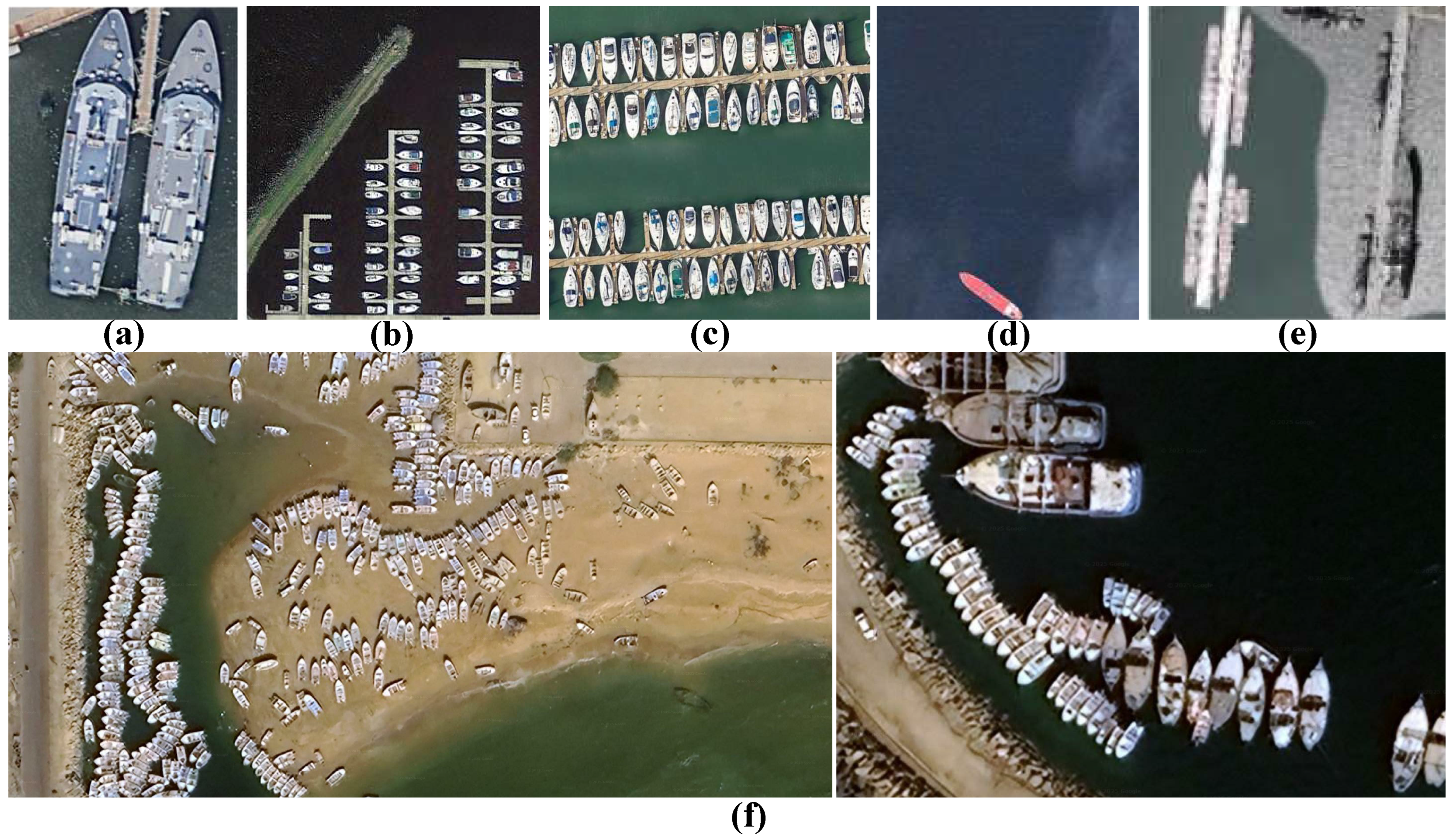
Figure 1. Comparison of the ship samples from satellite images in the existing benchmark datasets, (a) UoW-Vessel [42], (b) DIOR_SHIP [23], (c) DOTA-v2.0 [43], (d) LEVIR_SHIP [22], (e) HRSC2016 [20], and (f) the proposed MAKSEA dataset in this work.
Algorithms 19 00023 g001
Figure 2. Example images of the MAKSEA dataset.
Algorithms 19 00023 g002
Figure 3. A sample annotated image of MAKSEA dataset using QGIS. The annotated quadrilateral bounding boxes are shown with red color.
Algorithms 19 00023 g003
Figure 4. The overall architecture of the proposed model.
Algorithms 19 00023 g004
Figure 5. Example images used for training of the models, where images in (a) are the resized 512 × 512 original satellite image patch inputs, (b) are quadrilateral bounding box annotations manually generated in QGIS (red boxes), and (c) are corresponding quadrilateral segmentation masks derived directly from the quadrilateral bounding boxes. These masks approximate vessel shapes for efficient annotation and are used as ground truth for training and evaluation.
Algorithms 19 00023 g005
Figure 6. Visualization of regularization Process: (a) original input image; (b) raw output vectors from the segmentation model; (c) regularized output vectors aligned with quadrilateral format (red boxes).
Algorithms 19 00023 g006
Figure 7. Qualitative comparison of the proposed model with different SoTA models on challenging samples from the DIOR_SHIP dataset [70], where (a) is the input images and (b) is the ground-truth masks. (c) U-Net [26], (d) U-Net++ [32], (e) DeepLabV3+ [34], (f) SegNet [33], (g) Seg-Former [35], (h) TransUnet [62], (i) MambaSegNet [70], and (j) our proposed MVSegNet model (outlined with a red frame), respectively. True positives (TP) are shown in white, true negatives (TN) in black, false positives (FP) in magenta, and false negatives (FN) in green.
Algorithms 19 00023 g007
Figure 8. Qualitative comparison of the proposed model with different SoTA models on challenging samples from the LEVIR_SHIP dataset [70], where (a) is the input images and (b) is the ground truth. (c) U-Net [26], (d) U-Net++ [32], (e) DeepLabV3+ [34], (f) SegNet [33], (g) Seg-Former [35], (h) TransUnet [62], (i) MambaSegNet [70], and (j) our proposed MVSegNet model (outlined with a red frame), respectively. White and black colors denote TP and TN, respectively, while magenta and green indicate FP and FN.
Algorithms 19 00023 g008
Figure 9. Qualitative comparison of segmentation results on MAKSEA dataset. From left to right: (a) input image, (b) U-Net [26], (c) U-Net++ [32], and (d) our proposed MVSegNet method (outlined with a red frame).
Algorithms 19 00023 g009
Table 1. Statistic comparison of different high-resolution satellite image ship detection and segmentation benchmarks with our MAKSEA dataset.
DatasetsSource# ImagesPixel SizeClassResolution (m)BandYear
HRSC2016 [20]Google Earth1061Various sizes10.4–2RGB2016
DIOR_SHIP [70]Google Earth1258 800 × 800 10.5–30RGB2025
LEVIR_SHIP [70]Google Earth1461 800 × 600 10.2–1RGB2025
MAKSEAGoogle Earth8438 512 × 512 10.5–10RGBThis work
The symbol # Images denotes the number of images in the dataset.
Table 2. Comparison of training accuracy on the DIOR_SHIP dataset. Baseline results are reported from [70]. The best performances are illustrated in bold.
FrameworkIOUAccuracyPrecisionRecallF1-ScoreInference Time (ms)
Unet [26]0.76500.83200.80600.78200.794087.70
Unet++ [32]0.78800.84700.82900.84300.8239125.2
DeepLabV3+ [34]0.79230.85200.83000.85090.8403119.1
segNet [33]0.67000.86800.83800.86700.8609118.3
segformer [35]0.77910.87760.84410.87760.875861.90
TransUNet [62]0.82960.99030.92630.91140.9169174.0
MambaSegNet [70]0.82080.91760.92760.90760.917691.20
MVSegNet (Ours)0.86110.95420.96830.95340.960765.40
Table 3. Training accuracy comparison on the LEVIR_SHIP dataset. The results of other models are reported from [70]. The best performances are in bold.
FrameworkIOUAccuracyPrecisionRecallF1-ScoreInference Time (ms)
U-Net [26]0.59800.78100.74000.72500.732487.70
U-Net++ [32]0.73300.79700.83000.84500.8374125.2
DeepLabV3+ [34]0.77890.80300.80300.68300.7382119.1
segNet [33]0.68500.81600.81300.78500.7988118.3
segformer [35]0.56030.76060.72600.71060.718261.90
TransUNet [62]0.72920.99700.83460.83350.8177174.0
MambaSegNet [70]0.80940.85950.86950.89950.879591.20
MVSegNet (Ours)0.83240.87360.89240.91350.902865.40
Table 4. Performance comparison on the MAKSEA dataset. The best performances are shown in bold.
MethodmIoUDicePrecisionRecallAP
Mask-RCNN [31]0.6810.7430.7100.7230.694
FCN [30]0.6950.7610.7310.7330.711
U-Net [26]0.7230.8120.7840.7950.756
U-Net++ [32]0.7560.8340.8160.8230.789
DeepLabV3+ [34]0.7820.8510.8390.8410.815
SegNet [33]0.7640.8440.8280.8290.842
Seg-Former [35]0.7960.8500.8420.8380.826
Attention U-Net [63]0.7910.8590.8470.8520.823
TransUNet [62]0.8030.8680.8610.8630.839
SCUNet++ [40]0.7830.8620.8410.8490.822
MVSegNet (Ours)0.8260.8850.8790.8810.857
Table 5. Ablation study of different components on the prepared dataset.
ConfigurationIoUDicePrecisionRecallAP
Baseline (U-Net++)0.7560.8340.8160.8230.789
+ASPP0.7930.8620.8490.8530.827
+Attention Gates0.8120.8760.8650.8680.843
+Self-Attention0.8260.8850.8790.8810.857
Full Model (MVSegNet)0.8260.8850.8790.8810.857
Table 6. Attention mechanism analysis.
Attention ConfigurationIoUDicePrecisionRecall
No Attention0.7930.8620.8490.853
Attention Gates Only0.8120.8760.8650.868
Self Attention Only0.8050.8690.8570.861
Both Attention (MVSegNET)0.8260.8850.8790.881
Table 7. Segmentation performance of MVSegNet across different vessel size categories, measured using geodetic area computed on the WGS 84 ellipsoid. Ships are grouped into small (≤20 m 2 ), medium (20–200 m 2 ), and large (≥ 200 m 2 ) classes.
Size CategoryIoUDicePrecisionRecall
Small (≤20 m2)0.7810.8520.8430.847
Medium (20 m2–200 m2)0.8320.8890.8830.885
Large (≥200 m2)0.8450.8960.8910.893
Average0.8260.8850.8790.881
Table 8. Cross-dataset generalization performance.
TrainingTestingIoUDicePrecisionRecall
DIOR_SHIPMAKSEA0.6980.7670.7540.759
LEVIR_SHIPMAKSEA0.7120.7760.7680.771
MAKSEALEVIR_SHIP0.7890.8410.8670.892
MAKSEADIOR_SHIP0.8030.8610.8690.902
Table 9. Computational efficiency comparison of the proposed model among other SoTA standard architectures. The best performances are highlighted in bold.
MethodParams (M)FLOPs (G)Inference Time (ms)
U-Net [26]66.8021897.50
U-Net++ [32]79.40283136.2
DeepLabV3+ [34]34.20162104.1
Attention U-Net [73]41.5023878.70
TransUNet [62]105.3385182.3
Ours24.7011565.40
Disclaimer/Publisher’s Note: The statements, opinions and data contained in all publications are solely those of the individual author(s) and contributor(s) and not of MDPI and/or the editor(s). MDPI and/or the editor(s) disclaim responsibility for any injury to people or property resulting from any ideas, methods, instructions or products referred to in the content.