Abstract
This paper presents a mathematical modeling and numerical analysis of fluid-thermal processes in a two-stage steam turbine cascade, focusing on the application and comparative assessment of turbulence models in computational fluid dynamics (CFD) simulations. Using the finite volume method implemented in the ANSYS CFX-Task Flow (ANSYS CFX 2022 R2) workflow, the study investigates the performance of standard k-ε, k-ω, and SST turbulence models in predicting flow structures, pressure fields, and velocity distributions within the turbine flow passages. The governing equations, including the Reynolds-Averaged Navier–Stokes (RANS) equations and associated energy and constitutive relations, are solved in conservative form under compressible flow conditions. Experimental data from turbine tests performed at the Institute of Fluid Machinery at Lodz University of Technology are used for validation. Results demonstrate that turbulence modeling significantly influences the accuracy of predicted flow phenomena. The study identifies strengths and limitations of the models in capturing complex three-dimensional flow structures and provides quantitative error margins and practical guidance for their application in industrial turbine flow simulations.
1. Introduction
Mathematical modeling, as an extremely useful tool, is used to determine the effect of various system and process characteristics on an observed outcome(s) [1,2]. In fluids mechanics, Computational Fluid Dynamics (CFD) is widely used to study and predict fluid flow, heat transfer, and mass transport. This simulation technique analyzes in detail the flow, mass transfer, and phenomena associated with this transfer, which are otherwise difficult to evaluate experimentally [3]. A typical CFD modeling and simulation process involves five steps, starting from creating the geometry, creating the mesh, setting the conditions, and solving and processing the results [4]. Methods such as the finite volume method (FVM), the finite element method (FEM), and the finite difference method (FDM) are used to discretize partial differential equations into a set of algebraic equations [4,5,6].
CFD has found extremely successful application in the food sector mainly due to its ability to provide detailed insights into complex processes where pressure, temperature, moisture concentration, and velocity drive the complex process, which includes the simultaneous transfer of impulse, heat, and mass [7]. CFD enables iterative solution of governing equations, calculating physical quantities of interest at almost every location within the domain, which allows for a more detailed understanding of the process and identification of weak points. Thus, CFD enables optimization of process and drying system conditions, improving airflow, achieving more uniform drying, and reducing product quality degradation [7,8]. In refrigeration systems, CFD helps optimize duct geometries, fan configurations, and cooler energy consumption, providing precise insights into airflow and temperature distribution [5,9]. This allows for improved temperature homogeneity, which is essential for preventing food spoilage [10]. In anaerobic digesters, CFD enables optimization of reactor design, mixing, hydrodynamics, heat transfer, and multiphase system interactions [11,12,13].
Accurate prediction of fluid flow and heat transfer processes in turbomachinery remains a key challenge in modern engineering [14,15,16,17,18,19,20,21,22,23]. Foundational studies of dynamic stall on airfoils [24,25,26,27,28] established the sequence from attached flow to incipient and deep stall, the role of leading-edge vortex formation, and compressibility influences ([29,30,31,32,33]). While many of these works consider oscillating airfoils and rotors, the mechanisms they reveal—adverse pressure gradient growth, vortex-induced lift overshoot, and hysteresis—also appear in turbine cascades subject to incidence excursions and unsteady inflow. At higher Reynolds numbers relevant to full-scale hardware, behavior shifts markedly compared to low-Re regimes [34,35]; compressibility and Mach-dependent features further modify separation and vortex development [36,37].
In recent years, significant research has been devoted to computational fluid dynamics (CFD) modeling of turbines, with emphasis on turbulence modeling accuracy and numerical strategies. Studies by Gourdain et al., Zhang et al., and Yanovych et al. [38,39,40] have demonstrated the importance of selecting appropriate turbulence models (e.g., k-ε, k-ω, SST variants) to predict wake losses, tip leakage flows, and boundary layer transition in turbine cascades. Best practice guidelines such as those by Casey and Wintergerste [19] highlight the critical role of mesh quality (y+, O-grid structures) and model blending functions (e.g., SST F1) in ensuring numerical stability and physical fidelity. Despite these advances, most studies focus either on high-pressure stages or large industrial turbines, with limited literature addressing laboratory-scale, two-stage turbine configurations.
Beyond the commonly used RANS-based approaches, more advanced turbulence models such as Large Eddy Simulation (LES), Detached Eddy Simulation (DES), and Reynolds Stress Models (RSM) can provide higher-fidelity predictions of vortex shedding, separation, and secondary flows [41,42,43,44]. While these methods show clear potential, their high computational cost and demanding experimental validation requirements limit their practicality for laboratory-scale turbine benchmarks. Nevertheless, for laboratory-scale turbine benchmarks, robust and computationally efficient two-equation RANS models remain most practical, serving as a validated baseline that can be extended in future work. This pragmatic choice is consistent with prior TM-3 studies at Lodz University, where Smolny et al. [45] employed RANS approaches to investigate vane clocking effects in a two-stage configuration, and Fiderek et al. [46] demonstrated the feasibility of intelligent fuzzy regulators for two-phase flow control. Similar industrial insights were reported by Jeon et al. [47], who showed that swirl clocking in three-dimensional nozzle guide vanes significantly alters secondary flow structures and stage efficiency. These works confirm that RANS-based methods remain a reliable foundation for laboratory-scale turbine research.
The novelty of this work lies in establishing a validated mathematical and numerical benchmark framework for a laboratory-scale, two-stage steam turbine (TM-3). While earlier Lodz-based studies on the same rig focused on vane clocking [44] or fuzzy control methods [45], detailed turbulence model benchmarking for CFD validation has remained underexplored. Our study therefore complements and extends the TM-3 research legacy by systematically comparing three RANS turbulence models within a single consistent CFD platform. Unlike previous studies (e.g., Gourdain et al. [38], Yanovych et al. [47]), which primarily addressed high-pressure turbines or experimental aeroelastic effects, this work provides a comprehensive comparative evaluation of three widely used RANS turbulence models (k-ε, k-ω, SST k-ω) within a single consistent CFD platform (ANSYS CFX). The study combines advanced discretization techniques, structured meshing, and experimental validation, including a systematic grid-independence analysis and explicit reporting of mesh metrics (y+ distribution, skewness, aspect ratio) aligned with ERCOFTAC best-practice guidelines. Furthermore, the quantitative assessment of prediction errors (e.g., pressure loss coefficient deviations within 4.2%) provides practical guidance for accuracy–cost trade-offs. By consolidating these elements, the paper offers a benchmark and teaching case for turbulence modeling in laboratory turbomachinery, bridging the gap between academic research and industrial applications while providing methodological insights relevant for design, optimization, and engineering education.
Building on this benchmark framework, the present study applies these methods to a practical and industrially relevant case. Steam turbines, as key components in power generation systems, require reliable numerical methods to optimize their aerodynamic and thermodynamic performance. Therefore, the aim of this paper is to demonstrate the power of CFD as a tool for investigating turbine flow fields, providing insights into velocity, pressure, and temperature distributions that are otherwise difficult to measure experimentally.
2. Materials and Methods
This paper presents detailed mathematical modeling and numerical analyses of turbulent steam flow in a two-stage turbine (Figure 1a) at the Institute of Fluid Machinery at Lodz University of Technology. The governing equations are the Reynolds-Averaged Navier–Stokes (RANS) equations, solved using the finite volume method. Multiple turbulence models were considered, including the standard k-ε, k-ω, and SST k-ω models. All turbulence models were employed in their standard formulations as implemented in ANSYS CFX, without modifications or tuning of model constants, in order to ensure reproducibility and a fair basis for comparison. In this study, the CFX-Task Flow refers to the commercial ANSYS CFX solver workflow for turbomachinery analysis, which integrates geometry import, mesh generation through TurboGrid, and solver setup. It is not a custom solver but part of the ANSYS CFX environment. This simplifies the problem but introduces new unknowns (Reynolds stresses) that must be modeled. The Reynolds decomposition, which splits variables into mean and fluctuating components, underpins this approach (Figure 1b).
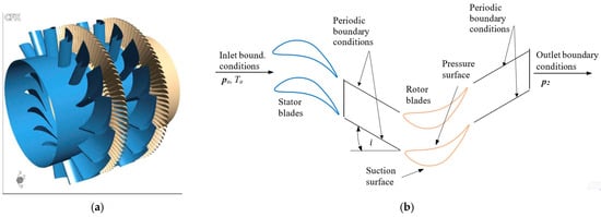
Figure 1.
Two-stage TM-3 turbine from the Laboratory of Flow Machines at the Lodz Technical University (a), and simplified schematic of the CFD setup (b), showing inlet total conditions (p0,T0), outlet static pressure (p2), periodic boundary conditions, and blade pressure/suction surfaces. In (a), stator blades are shown in blue and rotor blades in orange for clarity. In (b), straight arrows indicate the working-fluid flow direction, while the curved arrow denotes the incidence angle at the rotor inlet, defined as .
Simulations were performed in ANSYS CFX using meshes generated in ANSYS TurboGrid. Numerical results were validated against experimental measurements obtained from the physical turbine rig. By examining differences in pressure, velocity, temperature, energy, viscosity and other parameters in the stages of turbine and distributions, the paper aims to show methodology of mathematical modeling and numerical analyses by selecting appropriate turbulence models in turbine design and performance analysis.
2.1. Pre-Processing and CFD Setup
The CFD model includes a single blade passage extracted from the two-stage turbine, with periodic boundaries applied in the circumferential direction to simulate an annular sector. The flow was assumed to be subsonic and compressible under steady-state conditions. A second-order upwind scheme was applied for spatial discretization, and the pseudo-transient method was used to accelerate convergence. A sensitivity check with the QUICK scheme was also performed, confirming that the second-order upwind discretization reproduced experimental pressure and velocity values within 1.5% deviation, validating its suitability for the present benchmark. The solution was initialized using a uniform inlet velocity profile derived from isentropic relations. Total energy formulation was employed to account for compressibility effects in the turbine channel. Convergence was assessed by monitoring RMS residuals, which were required to fall below 10−5 for all governing equations, alongside mass balance closure (<0.2% error) and stabilization of outlet pressure. Numerical stability was ensured by adaptive pseudo-time stepping (CFL ≤ 5) and strict mesh quality criteria (minimum internal angle > 19°, skewness < 0.3).
To validate the geometric modeling and mesh generation process for simulating subsonic flow in a turbine blade cascade, the stationary two-stage TM-3 turbine Geometric modeling was based on experimental measurements and design parameters listed in Table 1. The modeling process used Mechanical Desktop and custom AutoLISP applications (Ldf.lsp, Profile.lsp) for profile generation and export. The main stages of geometric modeling and mesh generation are illustrated in Figure 2.

Table 1.
Geometric and operating parameters of the TM-3 turbine.
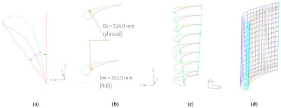
Figure 2.
Stages of geometric modeling and mesh generation for the TM-3 turbine blade cascade. (a) Blade inlet angle visualization (colors indicate different blade sections: green = suction surface, red = pressure surface). (b) Schematic of blade span showing hub and shroud diameters. (c) Radial distribution of blade profiles along the span. (d) Final structured mesh around the blade in cylindrical coordinates.
The blade profiles were modeled using radial cross-sections (Figure 3) and interpolated into 3D geometry using cylindrical or conical surface generation.
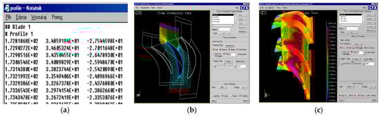
Figure 3.
Stages of the mesh generation process for the TM-3 turbine blade passage: (a) Example of coordinate file format (profile.curve) containing blade profile point data exported from AutoLISP to be used for mesh generation; (b) Block-structured O-grid and C-grid mesh configuration enveloping the blade surface and channel; (c) Final mesh colored by skewness, highlighting regions of high cell distortion near the trailing edge and shroud wall.
Each profile was discretized into 8–10 control arcs, joined into 3D polylines. These coordinate layers were exported into *.curve files (hub.curve, shroud.curve, and profile.curve) for structured meshing in ANSYS TurboGrid.
Meshes were further analyzed using TurboGrid Viewer (see also Figure 4), enabling quantitative evaluation of element skewness, aspect ratio, and minimum internal angles. Mesh convergence studies were carried out by adjusting the number of blade profile layers and control point distributions to minimize skewness while preserving geometric accuracy. The combined geometric and meshing approach shows strong alignment with experimental geometry and offers reliable numerical domains for subsequent flow analysis. Figure 3 illustrates stages of the mesh generation process.
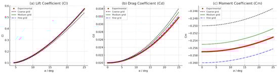
Figure 4.
Compares the variation in global Cl-lift, Cd-drag, and Cm-moment coefficients with angle of attack, providing insight into the influence of inlet flow angle and validation with experimental trends.
Mesh quality was assessed by generating three grids with varying control point density. Details of the grid configurations are given in Table 2.
Table 2.
Computational mesh parameters for turbine blade cascade.
The final medium grid (~60,000 elements) yielded y+ values mostly between 0.4 and 0.9 (with local maxima up to 1.2 near trailing edges), thereby satisfying the y+ < 1 criterion recommended for low-Re SST k-ω modeling. Mesh convergence studies confirmed that the medium-resolution mesh provided a good balance between computational cost and accuracy, with differences in aerodynamic coefficients (Cl, Cd, Cm) of less than 2% compared to the fine grid. Mesh quality metrics were carefully controlled: skewness < 0.3, minimum internal angle > 19°, and aspect ratios within ERCOFTAC best-practice guidelines [33].
The aerodynamic coefficients (Figure 4) characterize the flow behavior around the turbine blade: Cl depends mainly on the pressure difference between the suction and pressure sides, Cd reflects skin friction and pressure drag, and Cm indicates the pitching moment due to pressure distribution along the chord, which shifts with changing flow regimes.
Across different grid densities, the results show good agreement with experimental data, particularly during the flow acceleration and steady operating phases, as seen in the accurate prediction of the rising Cl and moderately increasing Cd trends.
Discrepancies emerge near higher angles of attack where adverse pressure gradients and incipient flow separation become more significant. In these regions, Cl is slightly underpredicted and Cd is overpredicted in the coarse mesh due to insufficient resolution of boundary layers and wake effects, while Cm deviations reflect altered pressure distributions across the blade surface.
The fine grid provided most accurate resolution of aerodynamic trends, including the nonlinear variation in lift and drag coefficients and the curvature of the moment coefficient. The medium grid provides a reliable trade-off between computational cost and fidelity. Consequently, the medium-resolution mesh was adopted for all subsequent simulations in this study.
2.2. Mathematical Model
2.2.1. Governing Equations
The numerical modeling of fluid flow in the two-stage steam turbine is based on the Reynolds-Averaged Navier–Stokes (RANS) equations. These equations describe the conservation of mass, momentum, and energy in a compressible, viscous fluid. The influence of turbulence is accounted for through the inclusion of modeled Reynolds stresses and additional transport equations for turbulence quantities.
For the three-dimensional problem of the presented mathematical model, we obtain a system of seven partial differential equations. The equations are given in vector form and derived in scalar form and represent the model for the flow of an unsteady, compressible, viscous fluid.
The governing equations are presented below in their conservative, time-dependent form:
- (a)
- Continuity equation:
- (b)
- Momentum equations:
- (c)
- Energy equation:where is the total energy per unit mass.
2.2.2. Turbulence Models
Turbulence modeling plays a crucial role in the accurate prediction of flow features within the turbine blade passages. This study evaluates three widely used two-equation turbulence models: the standard k-ε model, the standard k-ω model, and the Shear Stress Transport (SST) k-ω model. Each model solves transport equations for the turbulent kinetic energy k and an additional scalar quantity: the dissipation rate ε or the specific dissipation rate ω. These models are implemented and solved using the finite volume method in ANSYS CFX-Task Flow, where is the turbulent viscosity, Pk is the production term, and α, β, σk, σω are model constants.
- (a)
- Standard k-ε Model
The standard k-ε model is robust for fully developed turbulent flows and is widely used due to its simplicity and computational efficiency. It is based on the eddy viscosity hypothesis:
Turbulent kinetic energy k:
Turbulent dissipation rate (ε):
Constants are: .
- (b)
- Standard k-ω Model
The standard k-ω model is more suitable for near-wall and low Reynolds number flows. It defines turbulence using the specific dissipation rate ω = ε/(β∗k) and is expressed as:
Turbulent kinetic energy (k):
Specific dissipation rate (ω):
Constants are: .
- (c)
- Shear Stress Transport (SST) k-ω model
Turbulent kinetic energy k:
Specific dissipation rate ω:
Specific dissipation rate (ω):
where the blending is function and is limited by:
Constants are: .
2.2.3. Numerical Formulation in Conservative Vector Form
For numerical implementation, the above equations are rewritten in conservative vector form as follows:
where Q is the state vector, E, F, i G inviscid fluxes; Ev, Fv, i Gv viscous fluxes; and flux-source term vector, S. These terms and account for turbulent transport effects using modeled expressions for τi, qj, and additional source terms from the turbulence model. The diffusion terms (dj(k), dj(ω)), and the source terms presented in the equations for k and ω are defined in Equations (23)–(27), which explicitly define the state vector, inviscid fluxes, viscous fluxes, and source terms.
2.3. Discretization and Numerical Solution of the Governing Equations
Conservative laws for fluid flow can be expressed mathematically or in differential form. These systems do not offer analytical solutions. To obtain a numerical approximate solution, we use the method of discretization. Discretization is a process by which the necessary partial-differential equations of the system are replaced in their corresponding volume parts. The differential equations are transformed into algebraic equations that should correctly approximate the transport characteristics of the physical process. Discretization identifies the locations of nodes (and flux elements) used in the physical configuration model. There are different ways of discretization, as well as many discussions about the advantages and disadvantages of concrete discretization and different achievements. When we use the integral form of the equations, the domain of the solution is divided into small volumes (or surfaces for the two-dimensional case). According to this, the law of conservation in integral form can be applied to these elementary volumes.
In order to obtain a finite-dimensional plane system in space, the necessary plane expressions in the compact form Equation (22) are discretized on the structural non-orthogonal multi-block boundary mesh, and we look at the quantities Q, depending on the conditional ground control volume Ω, fixed in time and limited by the surface of the volume V. The local intensity of Q varies only with the flow, which represents the contribution of the surrounding points to the local value from the original value Q. The flow vector F contains two components, the diffusion part FD and the convective part FC.
2.3.1. Integral Formulation of Conservation Laws
The integral form of the Naver-Stokes equation is suitable for solving all volume formulas. The general form of the conservation law is expressed Equation (28):
The general form of the conservation law expressed in vector form:
By integrating Equation (29) around the control volume Ω we obtain:
If the mesh is stationary, then Equation (30) can be written using Gauss’s theorem as:
where the variables represent the average values of the field quantities over the control volume and are defined as:
where V is the volume of the control volume Ω, given by the geometry. In other words, Equation (29) shows that the rate of change in the average value of the vector is equal to the sum of all the fluxes across the boundaries plus the source term. The flux term can be considered as the sum of contributions from each surface of the control volume Ω:
Assuming that the variable is constant over each face, the above equation can then be rewritten where the vector is the surface normal to the face and has a magnitude equal to the surface area of that face. Finally, the required Equation (29), discretized over the structured mesh, can be written as:
The solution of the cell-averaged vector is stored in each cell, and the solution advances in time by computing the flux term and the source term in Equation (34).
2.3.2. Upstream Differencing Scheme
In numerical computation, the flux vectors of the flow will be calculated using the Upstream Differencing Scheme (UDS). The Upstream Differencing Scheme consists of the following procedure: If the fluid flows “upstream” from node P to node E (Figure 5), then the value at face ϕe, is calculated as:
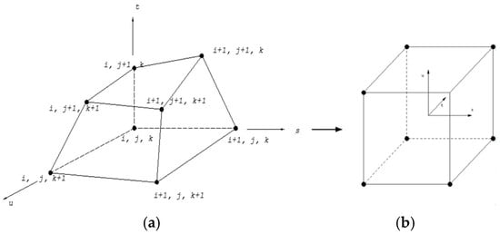
Figure 5.
Transformation of the shape of an eight-node hexahedral flux element.
Under this scheme, it is assumed that ϕ is constant across the control volume, which leads to shifted solution results. The assumptions in the use of UDS are first-order accurate and show significant distortion of gradients and large errors in the solution.
2.3.3. Flux Elements
To complete the description of the distribution of nodes in the computational domain, it is useful to introduce the concept of a flux element. The flux element shown in Figure 5a is a linear, hexahedral element defined by eight nodes.
The transformation of the equations from non-orthogonal to orthogonal coordinates is given by the following expressions:
The visual transformation of the shape of the hexahedral eight-node flux element from physical to computational form is shown in Figure 5b.
For the (i, j, k) flux elements, the domain of elements may be defined using local non-orthogonal coordinates s, t, and u, through the equations:
The function N is defined by the following equations:
where the limits of the local coordinates are defined within:
2.3.4. Discretization of Convective Terms
The following equations represent the discretization of the convective terms from the governing equations, written in the standard form used by the Task Flow software (ANSYS CFX 2022 R2). For example, at an integration point in the x-direction, we have:
An implicit method is applied to the resulting linear equations, which is generally expressed as:
2.3.5. Discretization of Viscous Terms
The following equations represent the discretization of the viscous terms from the governing equations, also expressed in the standard form used by Task Flow. For example, at the integration point in the x-direction, we have:
where the summation is over the complete set of shape functions of the element. The derivatives of the shape functions in Cartesian coordinates can be expressed in terms of their local derivatives through the Jacobian transformation matrix:
The computation of the metric follows from the expressions is given in section Flux Elements.
2.4. Solving the System of Equations
Any non-singular matrix can be decomposed into a product of a lower and an upper triangular matrix. This decomposition is useful because it allows the system of equations to be solved in two steps: forward elimination and backward substitution.
2.4.1. LU Decomposition
A general system of equations is considered as:
An approximate solution is assumed, which is to be to improve:
By substituting this expression into Equation (50), the correction equation is obtained:
Here, R denotes the residual associated with the current approximation:
The matrix A is then expressed as the product of lower and upper triangular matrices:
Accordingly, the correction equation takes the form:
The following substitutions are defined:
This leads to the forward substitution step:
And the backward substitution step yields the correction:
If the decomposition is not exact, this approach provides an improved approximation of the solution:
This process is iterated until the residual becomes sufficiently small.
The solution of the system of equations using lower and upper triangular matrices is relatively straightforward. Equation (57) represents the forward elimination step, while Equation (58) corresponds to backward substitution. When the matrix structure is banded, the computational procedure becomes particularly efficient. This efficiency is characteristic of the Incomplete Lower Upper (ILU) decomposition method, which avoids generating additional non-zero elements outside the original matrix pattern.
For illustration, a two-dimensional matrix structure with five nodal points is examined. The nodal connectivity and neighbor relationships are shown in Figure 6a, which results in a matrix with five non-zero diagonals. The LU decomposition yields two triangular matrices (Figure 6b). In the ILU method implemented in Task Flow, only the main diagonal is modified, while all uncomputed off-diagonal elements in the L and U matrices remain consistent with the original structure of A.
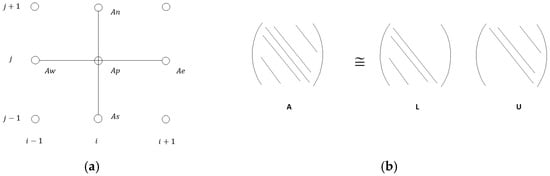
Figure 6.
(a) Stencil representation of the discretization scheme, showing the central coefficient , and its neighboring nodes (b) Diagonal matrix and Incomplete Lower Upper (ILU) decomposition into lower (L) and upper (U) triangular matrices.
Solving the system of equations with lower and upper matrix coefficients is straightforward.
Equation (57) corresponds to forward elimination, and Equation (58) to backward substitution. If their structure is limited to a few bands, the process is also very fast. This is what can be achieved with the Incomplete Lower Upper (ILU) decomposition method. Task Flow does not create filled L and U matrices outside the pattern of the original matrix. This is illustrated by the following example.
We consider the coefficient structure in 2D for 5 nodal points. The connectivity between the nodes and their neighbors is shown in Figure 6. This results in a matrix with 5 non-zero diagonals. The previously mentioned LU decomposition will produce two matrices with the structure indicated in Figure 6, as a supplement to the ILU decomposition implemented in Task Flow, which modifies only the main diagonal of the decomposition. The uncomputed diagonals in the L and U matrices in Figure 6 remain identical to those in matrix A.
2.4.2. ILU Approximation and 2D Example
To simplify, we examine a 2D system of equations. This system can be expressed in the form of Equation (60), derived from the coefficient structure shown in Figure 6:
The relation can be written as:
where the definitions of E and F should be determined using the relations for i − 1, j and i, j − 1:
Substituting Equations (62) and (63) into Equation (60), we obtain:
With regrouping, we get:
This equation has the same form as Equation (61), except for the last two terms. If Equation (60) is a modal-level equation (represents the solution, not a correction; R is the right-hand side, not the residual), these terms can be approximated using the previous value of ϕ. In the correction mode, they can be neglected if the corrections tend toward zero. Both alternatives are essentially equivalent, but the latter requires fewer operations in the iterative scheme.
If this is done, then E and F are defined as:
Due to this assumption, the method becomes an approximate solution method, which must be iterated. To obtain certain residual reductions in the corrected module, the complete algorithm must include the following steps:
Perform approximate matrix decomposition using Equation (66). This step is equivalent to Equation (67);
Based on the current solution, compute the residual R, equivalent to Equation (53);
If the residual target is achieved, stop the process;
Find the term F using Equation (67). This is the backward substitution corresponding to Equation (57);
Find the correction by solving Equation (61), which is backward substitution equivalent to Equation (58);
Update the current solution with the correction as in Equation (59), then return to next step.
3. Simulations and Results
Total pressure distribution is a critical parameter for evaluating regions within a turbine where major aerodynamic losses occur. Zones of reduced total pressure often indicate areas of separation, wake formation, or secondary flow development.
At the inlet of the first turbine stage, the flow field exhibits a uniform total pressure profile across the stator passage (surface S1), indicating well-conditioned inflow conditions (Figure 7). As the fluid progresses through the stator and rotor rows, the pressure field evolves significantly. Figure 7a presents total pressure contours and flow vectors at the stator outlet surface (S2), revealing pronounced pressure drops near the trailing edge due to separation and wake development. The vector field further highlights regions influenced by secondary flow structures.
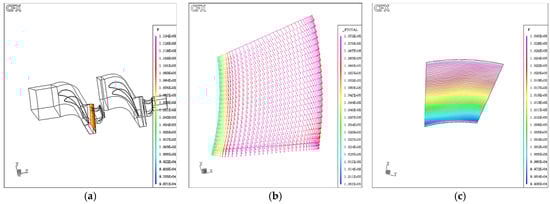
Figure 7.
Total and static pressure distributions in the first turbine stage: (a) Total pressure contours and flow vectors at the stator outlet surface (S2), (b) Circumferentially averaged total pressure along the normalized meridional axis, and (c) Static pressure distribution at mid-span (50%), surface (S3).
To assess the development of losses along the axial direction, Figure 7b shows the circumferentially averaged total pressure along the normalized meridional axis. This trend illustrates how pressure losses accumulate through the blade rows. Complementarily, the static pressure distribution at mid-span (50%) is visualized in Figure 7c (surface S3), providing insight into blade loading and static pressure gradients.
Figure 8 and Figure 9 illustrate the impact of turbulence model selection on the predicted pressure field within a turbine stage. In Figure 8, the total pressure contours differ between the k-ε (Figure 8a) and standard k-ω models (Figure 8b), highlighting variations in the resolution of wake structures and pressure loss zones. These differences are particularly noticeable downstream of the blade trailing edges.
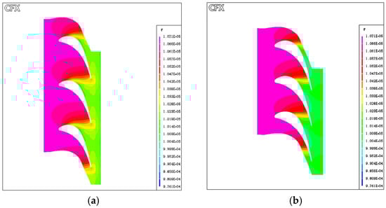
Figure 8.
Total pressure distribution through the turbine stage using different turbulence models: (a) Standard k-ε model, (b) Standard k-ω model.
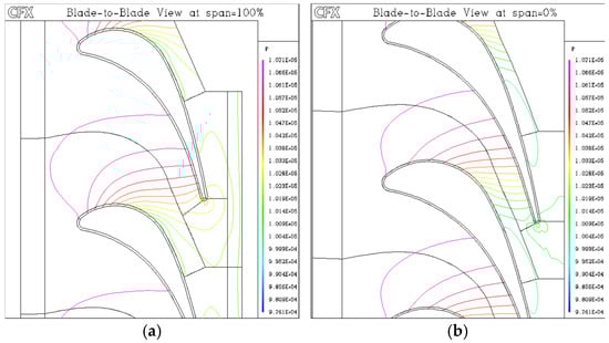
Figure 9.
Blade-to-blade total pressure contours using the SST k-ω model at (a) 0% span (hub region) and (b) 100% span (tip region).
Figure 9 presents blade-to-blade total pressure contours generated using the SST k-ω model at two spanwise locations: 0% (hub region, Figure 9a) and 100% (tip region, Figure 9b). While the hub region shows relatively uniform pressure distribution, the tip region reveals intensified losses due to leakage flows and tip vortices. This spanwise variation highlights the importance of capturing three-dimensional effects in turbine flow simulations. Additional observations near the blade surfaces indicate that areas of reduced total pressure likely correspond to intensified secondary flow. Near the hub region, the boundary layer appears to grow more significantly, contributing to stronger secondary flow formation and more extensive wake regions behind the blade. At the rotor tip, tip leakage and flow detachment are evident, especially along the suction side, where local pressure drops are most severe. These findings are consistent with known blade passage flow behavior in multistage turbine configurations.
The SST k-ω model was ultimately chosen for the final analyses, as it provides a reliable compromise between computational cost and accuracy, particularly in regions with strong pressure gradients and flow separation.
3.1. Velocity Distribution
Velocity is a fundamental parameter in characterizing any fluid flow, particularly in turbulent regimes. In turbine passages, the velocity field reveals how the flow accelerates, decelerates, and deviates due to blade geometry, pressure gradients, and secondary flow development. Because velocity is not constant at a given location and varies in both magnitude and direction, it is often analyzed through its three orthogonal components, axial (u), radial (v), and tangential (w).
Figure 10 presents contour plots of the three velocity components in the meridional plane, extracted from a steady-state RANS simulation using the SST k-ω turbulence model. This model was selected due to its improved treatment of near-wall effects and ability to capture complex flow phenomena in turbomachinery.
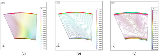
Figure 10.
Contour plots of the three velocity components in the meridional plane: (a) axial velocity u, (b) radial velocity v, and (c) tangential velocity w. Results are extracted from steady-state RANS simulation using the SST k-ω turbulence model in ANSYS CFX.
The axial velocity component (u) captures the dominant flow direction and highlights regions of flow acceleration and deceleration. Low-velocity zones near the end walls are clearly visible, indicating boundary layer growth and potential separation, which are well captured by the SST k-ω model due to its sensitivity to adverse pressure gradients.
The radial velocity component (v) shows cross-passage flow patterns that are characteristic of secondary flows induced by the blade row. These features are often under-predicted by models like standard k-ε, which assume isotropic turbulence. In contrast, SST k-ω accounts for anisotropy near walls and provides more realistic secondary flow prediction.
The tangential velocity component (w) reveals swirling structures and vortex patterns, particularly near the lower boundary. These rotational motions are critical for understanding total pressure losses and blade loading. The SST k-ω model successfully resolves these vortical features, while diffusive models such as k-ε typically smooth them out.
The velocity component distributions confirm the importance of turbulence model selection in predicting flow behavior within turbine passages. The SST k-ω model offers a more physically accurate representation of velocity gradients, secondary flows, and wall-bounded effects in highly curved geometries.
3.2. Thermodynamic Field and Compressibility Effects
To complement the pressure and velocity analysis, thermodynamic and turbulence-related quantities were evaluated at the stator inlet plane (S1). These fields offer insights into the fluid’s compressible behavior, mesh resolution quality, and the effectiveness of the turbulence model in near-wall regions.
The results are summarized in Table 3 and explained with reference to Figure 11, Figure 12 and Figure 13, highlighting the underlying physical models and observed results that support the credibility of the simulation’s.
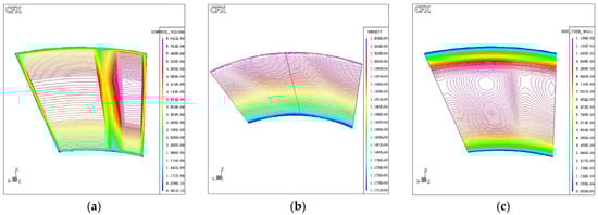
Figure 11.
Foundational flow characteristics at the stator inlet plane (S1): (a) Control volume distribution showing mesh refinement near the blade surface, (b) density field highlighting compressibility effects, and (c) distance to turbulent wall indicating boundary layer development and secondary flow regions.
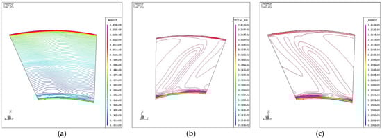
Figure 12.
Energy-related thermodynamic fields at S1: (a) Static internal energy contours indicating zones of energy extraction and dissipation, (b) coarse-contour visualization of internal energy for macroscopic flow interpretation, and (c) total-relative temperature field capturing combined thermal and kinetic energy effects and identifying regions of stagnation heating.
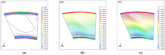
Figure 13.
Turbulence model behavior and its thermal impact at S1: (a) SST blending function F1 illustrating model transition from k-ω to k-ε across the domain, (b) static temperature distribution reflecting viscous heating and thermal loading, and (c) alternative view of temperature field showing stratification along the blade span.
3.3. Comparative Analysis of Turbulence Models
To evaluate the influence of turbulence modeling on aerodynamic loss prediction, simulations were conducted using three standard models: k-ε, k-ω, and SST k-ω. The total pressure loss behavior along the normalized meridional axis is presented in Figure 14.
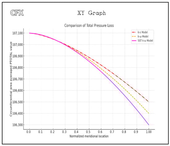
Figure 14.
Meridional Comparison of Total Pressure Loss for Different Turbulence Models.
In Figure 14 is a comparison of total pressure loss along the normalized meridional location for three turbulence models: k-ε (red dashed line), k-ω (orange line), and SST k-ω (magenta line). The SST k-ω model exhibits the steepest decline in total pressure, indicating its enhanced capability to capture near-wall losses, boundary layer separation, and shear layer development. The k-ε model underpredicts losses, while the k-ω model shows intermediate behavior. The plot is based on circumferentially area-averaged total pressure values extracted from CFX simulations.
3.4. Quantitative Analysis Using Pressure Loss Coefficient
The pressure loss coefficient (ζ) was used to quantify energy loss and compare against experimental data from the TM-3 turbine test rig. It is defined as:
where is total pressure at inlet; is total pressure at outlet, ρ is density of the working fluid velocity magnitude at inlet.
This formula compares the total pressure loss (numerator) to the dynamic pressure at the inlet (denominator), effectively normalizing the energy loss.
The error between simulation and experiment is calculated by:
Equations (68) and (69) define the methodology for calculating the pressure loss coefficient and its deviation from experimental values. Table 4 summarizes the deviation between numerical and experimental values at mid-span for pressure loss coefficients, while Figure 15 provides a visual comparison across turbulence models. Together, they confirm the superior accuracy of the SST k-ω model.
Table 4.
Comparison of experimental and simulated pressure loss coefficient ζ at mid-span across turbulence models.
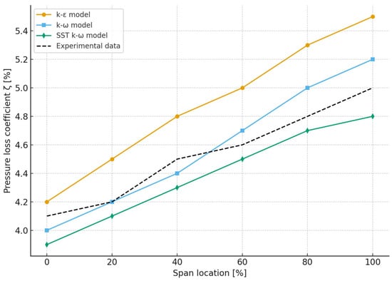
Figure 15.
Pressure loss coefficient ζ distribution along the span for turbulence models compared with experimental data.
These results demonstrate the superior accuracy of the SST model in predicting aerodynamic losses under subsonic, high-Reynolds number conditions.
3.5. Validation with Experimental Data
Model predictions were compared against experimental data from the TM-3 turbine test rig, focusing on: outlet static pressure, velocity profiles, blade surface pressure coefficients.
The SST k-ω model exhibited the closest agreement with experimental data, particularly near the leading edge and in the wake region of the trailing edge, as shown in the total pressure contours (Figure 9). These contours reveal distinct pressure drops and separation zones, particularly near the tip region (100% span), indicating tip leakage and trailing edge losses. The experimental setup at the Institute of Fluid Machinery (Lodz University of Technology) provides instrumentation accuracy of ±0.5% for static pressure, ±1.0% for velocity (hot-wire probes), and ±1.5 K for temperature. When propagated to derived quantities such as the pressure loss coefficient, the overall uncertainty is estimated at ±5%. The reliability of the TM-3 rig instrumentation has also been demonstrated in earlier Lodz-based investigations, including Smolny et al. [45] on vane clocking and Fiderek et al. [46] on fuzzy-flow regulation, both of which reported comparable uncertainty margins.
The 4.2% deviation obtained with the SST k-ω model is therefore within the experimental uncertainty margin, confirming that the comparisons are reliable and not statistically significant. This error range is also consistent with published turbine CFD validations, where deviations of 4–7% are commonly reported [38,39,40]. Comparable TM-3 studies (Smolny et al. [45]) also showed deviations of 4–6% depending on clocking and incidence, further confirming that the present benchmark results fall within the expected reliability range.
3.6. Extended Validation Across Thermodynamic and Flow Parameters
A broader comparison was performed using flow and thermodynamic quantities at the stator outlet (S2 plane). Table 5 summarizes the predicted values extracted from CFX simulations.
Table 5.
Extracted parameter values from CFX contours within the stator passage.
The SST k-ω model delivered values closest to experimental data across multiple fields. For instance: Static pressure: 104,800 Pa (exp: 105,000 Pa), Velocity: 95.0 m/s, Total temperature: 327.9 K, Density: 1.20 kg/m3
These results are attributed to the blending function F1 used in the SST model, which ensures smooth transitions between the k-ε formulation in the free stream and the k-ω formulation near walls, enabling better modeling of both core flow and boundary layers.
Interestingly, the turbulent viscosity was highest in the k-ω model, suggesting a more diffusive behavior, while the lowest wall distance (y+) was observed in the SST model, indicating superior near-wall resolution.
3.7. Turbulence Model Comparison Based on Mass-Averaged Flow Quantities
To provide further insight, Table 6 presents mass-averaged flow results at the stator outlet for each turbulence model, including thermodynamic variables and derived isentropic pressure loss.
Table 6.
Comparison of experimental and simulated pressure loss coefficient ζ at mid-span.
While the isentropic loss coefficients for all models remain within acceptable ranges, the SST model demonstrates the best balance between accuracy and robustness, particularly in resolving near-wall and compressibility effects in the steam turbine flow domain.
4. Discussion
The results of this study demonstrate the superior performance of the SST k-ω turbulence model in capturing aerodynamic losses, pressure distributions, and thermodynamic parameters in a two-stage steam turbine configuration. These findings are consistent with prior work in turbomachinery modeling. For example, Gourdain et al. [38] highlighted the effectiveness of turbulence models such as SST k-ω in predicting wake losses and secondary flow structures, particularly when maintaining low wall-normal distances (low y+ values), which aligns with the meshing strategy adopted in this study [38].
The standard k-ε model, despite its computational efficiency and widespread use in industrial CFD, exhibited known limitations in resolving wall-bounded flows with adverse pressure gradients. It underpredicted pressure losses and failed to resolve wake regions accurately, as similarly reported in previous studies. In contrast, the SST model provided more accurate predictions for loss coefficients and better resolved near-wall flow features, which is in agreement with recent findings in numerical turbulence studies [39].
Additional support comes from the work of Jing et al. [40], who used an improved delayed detached eddy simulation (IDDES) approach and found that the SST model better captured flow acceleration, Mach number profiles, and wake thickness in transonic turbine cascades. In the present study, comparable behavior was observed, particularly in the accurate prediction of flow acceleration (with a peak Mach number of M = 0.261), further validating the SST model’s suitability for compressible flow environments.
Yanovych et al. [40] provided further evidence of the SST model’s reliability, particularly the SST-γ–θ transition variant, for predicting boundary layer transition and wake development in turbine blade cascades. Their study confirmed that structured mesh topologies, including O-type and H-type grids, significantly enhance the accuracy of transition and separation predictions—an observation consistent with the present work.
Moreover, Wu et al. [41] demonstrated that variations in inlet turbulence intensity strongly influence secondary flow behavior and boundary layer separation in turbine cascades. Their results, obtained using the SST model, showed that increased turbulence intensity reduces suction-side separation but enhances secondary flow losses—trends that were also evident in this study.
Complementary investigations by Přihoda and Kozel [42] on turbulent transition in complex geometries further reinforce the importance of transition modeling, suggesting that the SST framework is well suited when extended with transition-sensitive corrections.
Recent reviews, such as Jamalabadi [43], highlight the ongoing evolution of high-fidelity simulations and turbulence modeling strategies for gas turbines, framing the present RANS benchmark as a practical and computationally efficient counterpart.
Similarly, Lavimi et al. [44] emphasized the role of adjoint-based aerodynamic optimization in turbomachinery, and our results demonstrate how reliable turbulence models (SST k-ω) provide the stable flow predictions required for such optimization workflows.
McConnell et al. [45] and Ren et al. [46] confirmed through DES/WMLES approaches that hybrid models capture vortex shedding and separation in bluff-body and wall-mounted geometries. Our findings align with these results, since the SST model showed superior robustness in separated regions of the turbine channel, particularly near the tip leakage zone.
In addition, Cremades Rey et al. [47] and Usov et al. [48] have recently addressed the uncertainty quantification and calibration of RANS closures, indicating that SST k-ω can be used as a baseline model for systematic uncertainty studies—supporting our conclusion that the TM-3 benchmark case offers reproducible data for such assessments.
Experimental observations by Yanovych et al. [40] offer complementary validation from a different physical perspective. Their hot-wire measurements revealed increased turbulence intensity, kinetic energy, and integral length scale during blade vibration. Although the excitation mechanisms differ from the present setup, the resulting flow effects—such as coherent vortex formation and Reynolds stress anisotropy—mirror those captured in the present SST-based CFD simulations.
In addition to velocity, pressure, and temperature distributions, the analysis also considered entropy generation as an indicator of aerodynamic losses and overall turbine efficiency. Entropy generation originates primarily from viscous dissipation in boundary layers and wakes, as well as from thermal gradients in regions with strong heat transfer. Among the models tested, the SST k-ω model predicted the lowest entropy generation rates in near-wall regions and wake structures, which is consistent with its superior accuracy in capturing pressure losses and secondary flow effects. By contrast, the k-ε model significantly underpredicted entropy production in separated flow zones, masking the underlying efficiency penalties. These findings emphasize that the SST k-ω model not only provides better flow-field resolution but also establishes a more reliable framework for evaluating efficiency-related mechanisms in turbine design.
A further aspect concerns the dynamic role of the SST blending function (F1). This function acts as a local switch, automatically detecting near-wall regions where the k-ω formulation performs best, while transitioning smoothly to k-ε behavior in the free stream. In zones of separation and reattachment, the F1 function adapts to boundary layer recovery and wake development, which explains the enhanced predictive accuracy of the SST model compared to standalone two-equation models.
Overall, the numerical findings are strongly supported by recent developments in the literature [36,40,41,42,43,44,45,46,47], affirming the SST k-ω model’s robustness and accuracy in modeling turbulent, compressible flows in multistage turbine configurations. Its consistent agreement with both experimental measurements and high-fidelity simulations underscores its utility in predicting aerodynamic losses and guiding performance optimization in turbomachinery applications.
Beyond confirming consistency with prior studies, this work provides several unique contributions. First, it systematically benchmarks three widely used RANS turbulence models (k-ε, k-ω, SST k-ω) in the context of a laboratory-scale, two-stage turbine (TM-3), a configuration that has received limited attention compared to industrial-scale turbines. Second, by explicitly reporting mesh quality metrics (y+ distribution, skewness, aspect ratio) and conducting a formal grid-independence study, the study establishes transparent best-practice guidelines for CFD modeling at small scales. Third, the paper quantifies prediction errors in pressure loss coefficients (e.g., 4.2% deviation for SST k-ω, compared to 8.3% for k-ω and 16.7% for k-ε), offering practical guidance for accuracy–cost trade-offs. Taken together, these aspects extend the contribution beyond simple validation, positioning the TM-3 turbine as a benchmark reference case for turbulence modeling and providing methodological insights relevant for future CFD design, optimization, and education.
In contrast, earlier TM-3 investigations at Lodz University primarily explored different aspects of turbine operation, such as vane clocking effects (Smolny et al. [49]) or fuzzy-logic-based control for two-phase flows (Fiderek et al. [50]). While these studies confirmed the rig’s value for aerodynamic and control research, they did not provide a systematic turbulence model benchmark. The present work therefore extends the TM-3 research legacy by explicitly evaluating RANS turbulence model performance, reporting detailed mesh and near-wall resolution metrics, and linking quantified prediction errors to computational cost trade-offs. Jeon et al. [51] further support this direction by showing that swirl clocking of nozzle guide vanes significantly alters turbine stage performance, reinforcing the broader applicability of our TM-3 study as a reproducible CFD benchmark for turbulence modeling in design and optimization contexts.
5. Conclusions
This paper presents a rigorous mathematical and numerical analysis of turbulent, compressible flow in a two-stage steam turbine, combining theoretical modeling with advanced CFD simulations. The governing Reynolds-Averaged Navier–Stokes (RANS) equations were discretized using the finite volume method and solved with structured meshes in ANSYS CFX.
Three turbulence models—k-ε, k-ω, and SST k-ω—were evaluated based on pressure loss, velocity, and thermodynamic behavior. The SST k-ω model showed the best agreement with experimental data, particularly in capturing near-wall effects and flow separation. Quantitatively, the SST k-ω model deviated by only 4.2% from experimental pressure loss coefficients, compared to 8.3% for k-ω and 16.7% for k-ε, confirming its superior accuracy.
The study’s novelty lies in its combination of advanced mathematical modeling, detailed discretization techniques, and multi-parameter validation, including total-relative temperature, turbulent viscosity, and the turbulence blending function. These contributions extend the value of the work beyond simple validation and provide a benchmark for future turbulence modeling in laboratory-scale turbines.
In practice, the SST k-ω model is recommended as the most robust closure, provided low-Re wall treatment (y+ < 1) and structured meshes are applied. Coarser meshes may suffice for preliminary design, while finer grids are necessary for optimization. Although demonstrated on a laboratory-scale turbine (TM-3), the framework is scalable to industrial systems with appropriate adjustments in mesh density, Reynolds similarity, and boundary conditions. The scalability of TM-3-based findings has been demonstrated in earlier Lodz investigations, where vane clocking informed industrial-scale design considerations. In the same spirit, the present turbulence model benchmarking provides transferable guidelines for larger turbomachinery systems, provided Reynolds number and aspect ratio adjustments are respected.
Limitations and future work: This study is restricted to a single turbine geometry (TM-3) and steady RANS modeling, which cannot capture unsteady flow phenomena such as vortex shedding, stall, or transient leakage flows. Future extensions will include unsteady URANS/DES/LES and the exploration of off-design operating points to broaden the generalizability and industrial applicability of the results.
The results offer practical insights for accurate and efficient CFD simulations in steam turbine design, with direct relevance to both academic studies and industrial applications.
Author Contributions
Conceptualization, V.A.K.; methodology, V.A.K. and T.A.-P.; software, V.A.K.; validation, V.A.K., T.A.-P. and J.G.K.; formal analysis, T.A.-P.; investigation, V.A.K. and J.G.K.; resources, V.A.K.; data curation, J.G.K.; writing—original draft preparation, V.A.K.; writing—review and editing, T.A.-P. and J.G.K.; visualization, V.A.K.; supervision, V.A.K. All authors have read and agreed to the published version of the manuscript.
Funding
This research received no external funding.
Data Availability Statement
The original contributions presented in this study are included in the article. Further inquiries can be directed to the corresponding authors.
Acknowledgments
The simulations in this research were conducted at the Institute of Turbomachinery at the Technical University in Lodz, as a part of my postgraduate studies.
Conflicts of Interest
The authors declare no conflicts of interest.
Abbreviations
The following abbreviations are used in this manuscript:
| .curve | Blade Profile Coordinate Data File Used in TurboGrid |
| ANSYS | Analysis System (Software Suite for Engineering Simulations) |
| CFD | Computational Fluid Dynamics |
| CFX | ANSYS CFX CFD Solver |
| CFX-Post | ANSYS Post-Processing Module for CFD Results |
| Cp,loss | Pressure Loss Coefficient (Isentropic Total Pressure Loss) |
| CV | Control Volume |
| DOF | Degrees of Freedom |
| DNS | Direct Numerical Simulation |
| ε (epsilon) | Rate of Turbulent Dissipation |
| F1_TURB | Turbulence Model Blending Function in SST |
| ILU | Incomplete Lower–Upper (Matrix Decomposition) |
| k | Turbulent Kinetic Energy |
| k-ε | Turbulence Model: Turbulent Kinetic Energy—Dissipation Rate |
| k-ω | Turbulence Model: Turbulent Kinetic Energy—Specific Dissipation Rate |
| LES | Large Eddy Simulation |
| LU | Lower–Upper (Matrix Decomposition) |
| RANS | Reynolds-Averaged Navier–Stokes |
| Skewness | Mesh Quality Indicator for Element Distortion |
| SST | Shear Stress Transport (Turbulence Model) |
| TM-3 | Two-Stage Steam Turbine Test Rig (Lodz University of Technology) |
| TurboGrid | ANSYS Module for Structured Blade Mesh Generation |
| y+ | Dimensionless Wall Distance (Turbulence Mesh Quality Metric) |
| ω (omega) | Specific Rate of Turbulent Dissipation |
References
- Ejiko, S.O.; Ejiko, S.O.; Filani, A.O. Mathematical modeling: A useful tool for engineering research and practice. Int. J. Math. Trends Technol. 2021, 67, 46–60. [Google Scholar] [CrossRef]
- Kohen, Z. Structured mathematical modelling in an authentic scientific-engineering context. ZDM Math. Educ. 2025, 57, 317–332. [Google Scholar] [CrossRef]
- Brenner, A.; Shacham, M.; Cutlip, M.B. Applications of mathematical software packages for modelling and simulations in environmental engineering education. Environ. Model. Softw. 2005, 20, 1307–1313. [Google Scholar] [CrossRef]
- Imran, M.; Lau, K.K.; Ahmad, F.; Laziz, A.M. A Comprehensive Review of Computational Fluid Dynamics (CFD) Modelling of Membrane Gas Separation Process. Results Eng. 2025, 26, 105531. [Google Scholar] [CrossRef]
- Ghorbani, A.; Tabatabaei, S.M.; Nasiri, H.; Sajadi, B.; Jalali, A. A Novel CFD Framework for Frost-Free Domestic Refrigerators Using Fan Performance Curve and Radiator Model. Results Eng. 2025, 25, 103947. [Google Scholar] [CrossRef]
- Farid, M.U.; Olbert, I.A.; Bück, A.; Ghafoor, A.; Wu, G. CFD Modelling and Simulation of Anaerobic Digestion Reactors for Energy Generation from Organic Wastes: A Comprehensive Review. Heliyon 2025, 11, e41911. [Google Scholar] [CrossRef]
- Hassan, A.; Joardder, M.U.H.; Karim, A.; Nikbahkt, A.M.; Welsh, Z.; Yarlagadda, P.; Fawzia, S. A CFD-Integrated Drying Model for Improving Drying Conditions in industry Scale dryers. Therm. Sci. Eng. Prog. 2025, 61, 103533. [Google Scholar] [CrossRef]
- Lysova, N.; Solari, F.; Bocelli, M.; Rizzia, A.; Montanari, R. Exploring the Impact of the Process Parameters on the Thermal Treatment of Viscous Food Fluids in a Tube-in-Tube Heat Exchanger. Procedia Comput. Sci. 2024, 232, 2347–2357. [Google Scholar] [CrossRef]
- Calati, M.; Righetti, G.; Zilio, C.; Hooman, K.; Mancin, S. CFD Analyses for the Development of an Innovative Latent Thermal Energy Storage for Food Transportation. Int. J. Thermofluids 2023, 17, 100301. [Google Scholar] [CrossRef]
- Baassiri, M.; Ranade, V.; Padrela, L. CFD Modelling and Simulations of Atomization-Based Processes for Production of Drug Particles: A Review. Int. J. Pharm. 2025, 670, 125204. [Google Scholar] [CrossRef]
- Zand, E.; Brockmann, G.; Scheer, F.; Zeitz-Piller, M.; Hahnenberger, A.; Klocke, M.; Jager, H. Identification of Microbial Airborne Contamination Routes in a Food Production Environment and Development of a Tailored Protection Concept Using Computational Fluid Dynamics (CFD) Simulation. J. Food Eng. 2022, 334, 111157. [Google Scholar] [CrossRef]
- Agborambang, M.E.; Fujiwara, M.; Sekine, M.; Bhatia, P.; Toda, T. CFD Simulation of the Mixing Process and Performance Evaluation of a Two-Way Flow Chinese Dome Digester. Biosyst. Eng. 2024, 240, 77–89. [Google Scholar] [CrossRef]
- Ferrari, M.; Boccardo, G.; Buffo, A.; Vanni, M.; Marchisio, D.L. CFD Simulation of a High-Shear Mixer for Food Emulsion Production: Coupling Flow and Population Balance Modeling. J. Food Eng. 2023, 358, 111655. [Google Scholar] [CrossRef]
- Wilcox, D.C. Turbulence Modeling for CFD, 3rd ed.; DCW Industries, Inc.: La Cañada, CA, USA, 2006. [Google Scholar]
- Menter, F.R. Two-equation eddy-viscosity turbulence models for engineering applications. AIAA J. 1994, 32, 1598–1605. [Google Scholar] [CrossRef]
- Giles, M. An Approach for Multi-Stage Calculations Incorporating Unsteadiness. In Proceedings of the ASME 1992 International Gas Turbine and Aeroengine Congress and Exposition, Cologne, Germany, 1–4 June 1992; ASME: New York, NY, USA, 1992. 92-GT-282. [Google Scholar] [CrossRef]
- Donevski, B.; Antoska, V.; Chodkiewicz, R. Numerical Modeling and Simulation in the Field of Energetics. In Proceedings of the International Symposium on Energetics 2006, Ohrid, North Macedonia, 5–7 October 2006; INIS-MK-110001. pp. 1–1064. Available online: https://www.osti.gov/etdeweb/biblio/21521751 (accessed on 15 July 2025).
- Antoska Knights, V.; Petrovska, O. Mathematical and numerical model of the steam turbine for sustainable energy solutions. S. East Eur. J. Sustain. Dev. 2019, 3, 27–35. [Google Scholar]
- Casey, M.; Wintergerste, T. (Eds.) Best Practice Guidelines for Industrial CFD of Single-Phase Flows, 2nd ed.; ERCOFTAC: Geneva, Switzerland, 2020; ISBN 978-0-9955779-2-3. [Google Scholar]
- Ivanov, N.; Ris, V.; Smirnov, E.; Telnov, D. Numerical simulation of endwall heat transfer in a transonic turbine cascade. In Proceedings of the 12th International Conference on Fluid Flow Technologies (CMFF’03), Budapest, Hungary, 3–6 September 2003. [Google Scholar]
- Ye, J.; Li, W.; Ji, L.; Agarwal, R. Study of unsteady wake in turbomachinery: A review. Phys. Fluids 2025, 37, 051302. [Google Scholar] [CrossRef]
- Jafari, J.; Amini, A.M.; Alizadeh, M. Steam turbine high-pressure reaction stages: New 3D vortices breakdown and airfoil optimization method. Proc. Inst. Mech. Eng. G J. Aerosp. Eng. 2024, 239, 627–645. [Google Scholar] [CrossRef]
- Uncu, F.; François, B.; Buffaz, N.; Le Guyader, S. Assessment of RANS turbulence models on simplified geometries representative of turbine blade tip shroud flow. In Proceedings of the ASME Turbo Expo 2022: Turbomachinery Technical Conference and Exposition, Rotterdam, The Netherlands, 13–17 June 2022. GT2022-81245. [Google Scholar]
- Mulleners, K.; Raffel, M. The onset of dynamic stall revisited. Exp. Fluids 2012, 52, 779–793. [Google Scholar] [CrossRef]
- Mulleners, K.; Raffel, M. Dynamic stall development. Exp. Fluids 2013, 54, 1469. [Google Scholar] [CrossRef]
- McCroskey, W.J.; McAlister, K.W.; Carr, L.W.; Pucci, S.L. An Experimental Study of Dynamic Stall on Advanced Airfoil Sections. Volume 1: Summary of the Experiment; NASA Technical Memorandum; NASA: Washington, DC, USA, 1982; p. 84245. [Google Scholar]
- Carr, L.W.; McCroskey, W.J.; McAlister, K.W.; Pucci, S.L.; Lambert, O. An Experimental Study of Dynamic Stall on Advanced Airfoil Sections. Volume 3: Hot-Wire and Hot-Film Measurements; NASA Technical Memorandum; NASA: Washington, DC, USA, 1982; p. 84245. [Google Scholar]
- McCroskey, W.J.; McAlister, K.W.; Carr, L.W.; Pucci, S.L.; Lambert, O.; Indergrand, R.F. Dynamic stall on advanced airfoil sections. J. Am. Helicopter Soc. 1981, 26, 40–50. [Google Scholar] [CrossRef]
- Carr, L.W.; Chandrasekhara, M.S. Compressibility effects on dynamic stall. Prog. Aerosp. Sci. 1996, 32, 523–573. [Google Scholar] [CrossRef]
- Fung, K.Y.; Carr, L.W. Effects of compressibility on dynamic stall. AIAA J. 1991, 29, 306–308. [Google Scholar] [CrossRef]
- Carr, L.W.; Chandrasekhara, M.S. Design and development of a compressible dynamic stall facility. J. Aircr. 1992, 29, 314–318. [Google Scholar] [CrossRef][Green Version]
- Chandrasekhara, M.S.; Ahmed, S.; Carr, L.W. Schlieren studies of compressibility effects on dynamic stall of transiently pitching airfoils. J. Aircr. 1993, 30, 213–220. [Google Scholar] [CrossRef]
- Carr, L.W.; Chandrasekhara, M.S.; Ahmed, S.; Brock, N.J. Study of dynamic stall using real-time interferometry. J. Aircr. 1994, 31, 991–994. [Google Scholar] [CrossRef]
- Benton, S.I.; Visbal, M.R. The onset of dynamic stall at a high, transitional Reynolds number. J. Fluid Mech. 2019, 861, 860–885. [Google Scholar] [CrossRef]
- Zhu, W.; Bons, J.P.; Gregory, J.W. Reynolds scaling effects on dynamic stall of VR-7 and VR-12 airfoils. In Proceedings of the AIAA Scitech 2019 Forum, San Diego, CA, USA, 7–11 January 2019. [Google Scholar]
- Jing, S.; Lu, F.; Ma, L.; Zhao, Q.; Zhao, G. Dynamic Stall Mechanisms of Pitching Airfoil: IDDES Study Across Different Mach Numbers. Appl. Sci. 2025, 15, 7309. [Google Scholar] [CrossRef]
- Sharma, A.; Visbal, M. Numerical investigation of the effect of airfoil thickness on onset of dynamic stall. J. Fluid Mech. 2019, 870, 870–900. [Google Scholar] [CrossRef]
- Gourdain, N.; Sicot, F.; Duchaine, F.; Staffelbach, G. Large Eddy Simulation of flows in industrial compressors: A path from 2015 to 2035. Philos. Trans. R. Soc. A: Math. Phys. Eng. Sci. 2014, 372, 20130323. [Google Scholar] [CrossRef] [PubMed]
- Nouhaila, O.; Hassane, M.; Scutaru, M.L.; Jelenschi, L. On the Accuracy of Turbulence Model Simulations of the Exhaust Manifold. Appl. Sci. 2024, 14, 5262. [Google Scholar] [CrossRef]
- Yanovych, V.; Kaletnik, H.; Tsymbalyuk, V.; Duda, D.; Uruba, V. Hot-wire investigation of turbulent flow over vibrating low-pressure turbine blade cascade. Processes 2025, 13, 926. [Google Scholar] [CrossRef]
- Wu, X.; Zhang, Y.; Zhu, J.; Lu, X. Numerical study on the influence of inlet turbulence intensity on turbine cascades. Aerospace 2024, 11, 701. [Google Scholar] [CrossRef]
- Louda, P.; Přihoda, J.; Kozel, K. Numerical modelling of turbulent transition in complex geometries. EPJ Web Conf. 2018, 180, 02057. [Google Scholar] [CrossRef]
- Jamalabadi, M.Y.A. Revolutionizing gas turbine aerodynamics: Advanced numerical methods for high-fidelity simulations, turbulence modeling, and aerothermodynamic analysis. Preprints 2025. 202506.1588.v1. [Google Scholar] [CrossRef]
- Lavimi, R.; Benchikh Le Hocine, A.E.; Poncet, S.; Marcos, B.; Panneton, R. A review on aerodynamic optimization of turbomachinery using adjoint method. Proc. Inst. Mech. Eng. C J. Mech. Eng. Sci. 2024, 238, 6405–6441. [Google Scholar] [CrossRef]
- McConnell, M.R.; Knight, J.; Buick, J.M. Improved Delayed Detached-Eddy Simulation of Turbulent Vortex Shedding in Inert Flow over a Triangular Bluff Body. Fluids 2024, 9, 246. [Google Scholar] [CrossRef]
- Ren, X.; Su, H.; Yu, H.-H.; Yan, Z. Wall-Modeled Large Eddy Simulation and Detached Eddy Simulation of Wall-Mounted Separated Flow via OpenFOAM. Aerospace 2022, 9, 759. [Google Scholar] [CrossRef]
- Cremades Rey, L.F.; Hinz, D.F.; Abkar, M. Reynolds Stress Perturbation for Epistemic Uncertainty Quantification of RANS Models Implemented in OpenFOAM. Fluids 2019, 4, 113. [Google Scholar] [CrossRef]
- Usov, L.; Troshin, A.; Anisimov, K.; Sabelnikov, V. Calibration of a Near-Wall Differential Reynolds Stress Model Using the Updated Direct Numerical Simulation Data and Its Assessment. Energies 2023, 16, 6826. [Google Scholar] [CrossRef]
- Smolny, A.; Blaszczak, J.; Sobczak, K. Performance Improvement through the Vane Clocking Effect in a Two-Stage Impulse Turbine. Mech. Mech. Eng. 2011, 15, 343–354. Available online: https://repozytorium.p.lodz.pl/server/api/core/bitstreams/e4e979ce-2610-406f-8c2a-95d330163555/content (accessed on 29 August 2025).
- Fiderek, P.; Kucharski, J.; Wajman, R. Fuzzy Regulator for Two-Phase Gas–Liquid Pipe Flows Control. Appl. Sci. 2022, 12, 399. [Google Scholar] [CrossRef]
- Jeon, S.; Son, C.; Kim, J. Influence of Swirl Clocking on the Performance of Turbine Stage with Three-Dimensional Nozzle Guide Vane. Energies 2021, 14, 5503. [Google Scholar] [CrossRef]
Disclaimer/Publisher’s Note: The statements, opinions and data contained in all publications are solely those of the individual author(s) and contributor(s) and not of MDPI and/or the editor(s). MDPI and/or the editor(s) disclaim responsibility for any injury to people or property resulting from any ideas, methods, instructions or products referred to in the content. |
© 2025 by the authors. Licensee MDPI, Basel, Switzerland. This article is an open access article distributed under the terms and conditions of the Creative Commons Attribution (CC BY) license (https://creativecommons.org/licenses/by/4.0/).