Abstract
With the rise in physiological data sampled from wearable devices, efficient methods must be developed to encode temporal information for the comparison of time series arising from uncontrolled monitoring. We present a fast, nonparametric method called Multiscale Average Absolute Difference (MSAAD) to extract multiscale temporal features from wearable device data for purposes ranging from statistical analysis to machine learning inference. MSAAD outperforms comparable algorithms like multiscale sample entropy (MSSE) and multiscale Katz Fractal Dimension (MS-KFD) in terms of calculation stability on short realizations and faster runtime. MSAAD outperforms MSSE and MS-KFD by being able to separate diabetic and non-diabetic cohorts with moderate and large effect sizes in both sexes. Furthermore, it is capable of capturing “critical slowing down” in the temperature dynamics of aging populations, a phenomenon that has been previously observed in controlled settings. We propose that MSAAD is a scalable, interpretable time series feature that is capable of identifying meaningful differences in physiological time series data without making assumptions regarding underlying process models. MSAAD could improve the ability to derive insight from time series data mining for health applications.
1. Introduction
With the rise in wearable device (wearables) users, there is a concomitant rise in the quantity of signal data being sampled from them [1]. These data provide novel opportunities to evaluate how environmental, behavioral, and medical factors affect physiological phenomena in large populations [2,3,4,5]. Specifically, they allow for the continuous evaluation of various health states in large, distributed populations which can be utilized for acute illness onset, chronic condition monitoring, or responses to physiological perturbations [6,7,8,9]. However, a challenge of population-scale analyses of physiological differences with wearables is that the data are sampled both longitudinally and at relatively high temporal resolution [10]. Given that physiological processes occur on timescales across several orders of magnitude (e.g., minutes to years), it is necessary to develop time series feature engineering that can leverage these physiological data for research or predictive purposes.
While the availability of large-scale wearable-generated data is relatively new, the field of time series analysis has a long history [11,12]. A common approach, which usually assumes some regularity to the signal, is Fourier analysis [13], where signals are decomposed into stationary sine waves of varying amplitudes, frequencies, and phases. However, biological systems are often not stationary (e.g., no two days are exactly the same) [14,15]. Deviation from signal regularity reflects the body reacting to complex inputs from the real world, and useful information might reside in the irregularities of these signals.
One popular approach to quantifying and analyzing these irregularities concerns the evaluation of process complexity [16]. Methods of time series complexity evaluation typically focus on process self-similarity (fractality) [17,18] non-linear dynamics [19,20,21], or entropy [22,23,24,25]. As each focus estimates different properties of a time series, it also makes assumptions about the underlying process behavior, and longitudinal physiological data cannot always be evaluated for if they meet these assumptions. Detrended fluctuation analysis (DFA) assumes a process with polynomial integrability [26]. Non-linear dynamics assumes the noise amplitude is low relative to the signal amplitude at a given time lag [27]. Entropy estimates of time series data assume stochastic processes with potential non-linear dependance from a sufficiently long time series [16]. These methods are often applied by researchers with domain expertise in the underlying signal of interest who understand the limitations of each method [28,29,30,31,32,33,34,35,36,37,38,39,40], and have been used for estimation of complexity in many physiological signals in controlled environments. However, the contexts in which longitudinal physiological data from wearables are typically captured often involve uncontrolled settings that are affected by person-level differences in physiological and behavioral activity [41], environmental perturbations [42], and sensor/device dissimilarities [43]. Wearables data are also bound to violate assumptions of stationarity and ergodicity that are often prerequisites for complexity interpretation [44]. Finally, while the aforementioned techniques have been useful in many applications, they tend to be computationally expensive. As data from wearables and other on-edge devices become incorporated into health monitoring systems [45,46], efficient processes are needed to allow distributed, real time analysis [47].
In this work, we demonstrate a computationally efficient, multiscale measurement of complexity that is inspired by the Katz Fractal Dimension (KFD) [48] and Multiscale Sample Entropy (MSSE) [49,50] that we call Multiscale Average Absolute Difference (MSAAD). We deploy this feature in both synthetic data and human longitudinal distal skin temperature data to show its performance and limitations in real world contexts, compared with KFD and MSSE for both information gain and efficiency. We use two real-world test contexts—a binary label of a complex condition (diabetes) and a continuous variable (age)—and find that in both contexts MSAAD provides greater separability at less computational cost than MSSE, and greater separability at similar cost compared with KFD.
2. Materials and Methods
2.1. Generated β Noise Realizations
To generate power-law noise realizations, we first produced a discrete white noise sequence of length , where (Python 3.11.5; numpy 1.24.4). The sequence was transformed into the frequency domain via the Fast Fourier Transform (FFT):
We then shaped the power spectrum to follow a power-law relationship of the form
By scaling the Fourier amplitudes as
To ensure comparable cumulative power between realizations, the Fourier amplitudes of were normalized as
These transformations ensured the resulting time-domain signals exhibited the desired spectral exponent while being similar in mean and variance. The power-law noise realization was obtained by applying the inverse FFT with randomly initialized phases:
For each value of , we generated 100 independent realizations . For each realization, we computed MSAAD and MSSE. With these collection of MSAAD and MSSE curves, we computed the median and standard deviation of all curves for each . To calculate the normalized standard deviation at each coarse-graining scale for the different processes, we z-scored each curve along the scale axis and calculated the variance of the average absolute difference (AAD) and Sample Entropy measurement at each scale. The variances over each 20-sample scale window were compared using non-parametric Mann–Whitney U tests.
2.2. Ethics Approval and Consent to Participate
The University of California San Francisco (UCSF) Institutional Review Board (IRB, IRB# 20-30408) and the U.S. Department of Defense (DOD) Human Research Protections Office (HRPO, HRPO# E01877.1a) approved of all study activities, and all research was performed in accordance with relevant guidelines and regulations and the Declaration of Helsinki. All participants provided informed electronic consent. We did not compensate participants for participation.
2.3. Wearable Device and Questionnaire Data Collection
All data were part of the TemPredict Study and were collected from January to November 2020 [51]. The dataset includes physiological data generated using the wearable device Oura Ring Gen2 [52] (Figure 1), as well as survey data such as self-reported sex, age, race, and ethnicity. The Oura Ring wireless device worn on the finger contains, among other things, a negative coefficient (NTC) thermistor (resolution of 0.07 °C) to detect distal body temperature. Wearable data were wirelessly synced via Bluetooth from the ring to the user’s smartphone when the Oura App was in use. Data from the app was then sent by the app to Oura’s cloud architecture, from which we received a one-time data push to our cloud storage located on San Diego Supercomputer (SDSC) infrastructure.
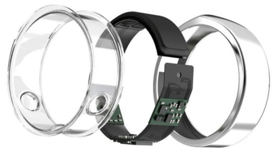
Figure 1.
An example technical image of an Oura Ring Gen2 device.
In addition to the wearable-generated data, participants were asked to answer a questionnaire related to chronic illness. Demographic questionnaire data included approximate age in years (“What is your age?”), sex (“What is your biological sex?”), ethnicity (“Are you of Hispanic or Latino Origin?”), race (Options: African American/Black, Asian, Caucasian/White, Middle Eastern, Native American/Native Alaskan, Native Hawaiian/Other Pacific Islander, South Asian, Other Ethnicity [optional text]). A medical conditions question (MCQ) asked “Have you ever been told by a healthcare professional that you have, or have been treated for, any of the following conditions (in the past or currently)?” with options “diabetes (not including pre-diabetes)” and “None of these” as potential options. The “None of these” options indicated the participant has, to their knowledge, not had or been diagnosed with any of the following conditions: high blood pressure or hypertension, diabetes, coronary artery disease or angina, a heart attack, congestive heart failure, stroke or transient ischemic attack, atrial fibrillation, sleep apnea, COPD (emphysema, chronic bronchitis), asthma requiring regular inhaler use, cancer, anemia or other blood disorder, immunodeficiency including HIV, or other respiratory issues.
2.4. Cohen’s d Estimate of Effect Size
Cohen’s d is estimated by measuring the difference between two group means and dividing that difference by the pooled standard deviation of both groups (pingouin 0.5.5). It can be interpreted as how many standard deviations the means of both groups are from each other. While only guidelines, prior published work establishes d values of 0.2, 0.5, and 0.8 to be small, medium, and large effect sizes, respectively.
2.5. Comparison of Cohorts Reporting the Presence or Absence of DM Dx
The absence (No DM Dx) or reporting of diabetes mellitus (DM Dx) were chosen as categorical test cases for MSAAD applied to temperature due to previously reported associations between diabetes mellitus and thermoregulation [53] caused by comorbid vascular disease [54] and peripheral neuropathy [55]. The cohort of individuals reporting DM Dx were filtered on the following criteria: ages between 45 and 65 as well as endorsing “Diabetes” in response to MCQ from the TemPredict survey. From that screening, 328 males and 145 females met these criteria (pandas 2.3.2). The choice of the 45 to 65 age range was made based on potential confounding factors of age.
For those not reporting a DM Dx, the criteria were as follows: ages between 45 and 65, lack of endorsement of “Diabetes” in response to the MCQ from the survey and positive endorsement of the “None of these” response option, which confirmed the absence of any of the conditions listed in the survey, and affirmed that they are not taking any medication. From that screening, 2034 males and 1683 females met these criteria.
The value to be compared between groups was the sum of the MSAAD curves. If a significant Kruskal–Wallis test identified that there was at least one significant comparison between a sex/condition comparison, post hoc Dunn’s tests with Bonferroni correction were performed to identify the specific significant pairs.
2.6. Comparison of Age Cohorts
The groups of age were chosen in 10-year increments ranging from 20 to 79 and separated by sex (e.g., Males aged 70–79; females aged 20–29). Individuals were filtered out if they did not have at least ten times as much data as the largest scale being used. For the age comparisons performed in this work the largest scale compared was 4096 min. The group with the most samples were males between the ages of 30 and 40 with 2684 individuals. The group with the fewest samples were males between the ages of 70 and 80 with 117 individuals. Because correlations between MSAAD measurements and age were used later, a random selection of 117 individuals from each age group for both females and males were used to ensure there was no biasing of the correlation to the group with the most samples. For each scale, Spearman’s correlation was used to identify a rank-order relationship between the AAD and age.
3. Results
3.1. Coarse Graining and Multiscale Average Absolute Difference
The coarse-graining procedure originates from Costa 2000 [49], where it was introduced to assess the dynamics of a time series across multiple temporal scales. Mathematically, this operation applies a non-overlapping moving average of length to the original time series, effectively acting as a low-pass filter. This process attenuates high-frequency noise and retains slower trends, enabling the analysis of structural patterns at varying resolutions. It can formally be expressed as
where is the number of samples being aggregated (coursing scale), is the index of the element that comprises samples, belongs to the time series set , and is the element of .
The computation of total line length, , reflects the cumulative first-order variation in the coarse-grained signal. Formally, this is equivalent to the norm of the first-order difference vector, which captures the absolute sum of local transitions across the time series. The total length of the curve, L, from is then computed as follows:
The line length is then normalized by the number of differences, producing the average absolute difference (AAD). This normalization yields a scale-invariant measure of local variability, sensitive to both the amplitude and frequency of transitions in the signal:
where is the line length at coarse-graining scale , is the i-th element of (Equation (1)), and is the size of . By evaluating AAD across multiple values, the resulting Multiscale Average Absolute Difference (MSAAD) curve characterizes how signal complexity evolves with scale, similar in motivation to Multiscale Entropy methods. An informal, pseudocode description of MSAAD can be found in Algorithm 1.
| Algorithm 1. A pseudocode description of the MSAAD algorithm. |
| Input: An ordered, discrete time series of any length and a list of integer scale sizes, s. Output: The MSAAD curve of the time series of the same length as the number of scales used
|
3.2. In Simulated Noise Processes, MSAAD Is More Stable than MSSE at Larger Bin Sizes and Approximates the Power Decay Constant for −1 ≤ β ≤ 2 Realizations
Prior to evaluating the performance of MSAAD in real-world physiological data, we first evaluated the behavior and stability of MSAAD and compared it to MSSE in various simulated 1⁄fβ noise processes (see Generated β Noise Realizations in Methods). MSAAD and MSSE we recomputed on 100 unique realizations for realizations with power law scaling of −2 ≤ β ≤ 2 (Figure 2A, Zoomed in pink noise in Figure 2B). MSSE approaches 0 Natural Units of Information (nats) for violet, blue, and white noise processes as scale increases, remains relatively constant for pink noise (β = 1), and increases for brown noise (β = 2) (Figure 2C Top Left); however, variance across the 100 realizations increases as the coarsing scale increases (shaded areas around the solid curves). A log-log representation of the same data reflects non-constant slopes for β ≤ 0 (Figure 2C Top Right). MSAAD shares similar long-term median behavior to MSSE as a function of scale size (Figure 2C Bottom Left). A log-log representation of the same data reflects a constant slope for all processes examined as the coarsing scale increases (Figure 2C Bottom Right). For β ≤ −1, MSAAD across multiple realizations has higher variance than MSSE when matched for scales < 20 samples (p < 0.001) (Figure 2D). However, MSAAD has lower variance than MSSE at all scales for β ≥ 0 (p < 0.001). Furthermore, the variance increases at a lesser rate than MSSE as scale increases (Figure 2E). The slope of log-log MSAAD relationships for smaller increments of β indicates a linear relationship between the MSAAD curve slope and the power decay constant of the test signals (Figure 3A) (p < 0.0001, R = 0.997). The relationship does not hold for more extreme negative values of the power decay constant and becomes weaker for decay constants greater than those for brown noise. The MSAAD calculation is more than 10 times faster than the MSSE calculation (Figure 3B).
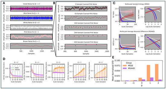
Figure 2.
(A). Example 1/fβ processes for violet, blue, white, pink, and brown noise (Note: the synthetic signals are unitless and thus MSAAD is also unitless). (B). Zoomed in effect of multiscale coarse graining on the pink noise timeseries. (C). Top. Multiscale Sample Entropy curves in normal and log scales. Bottom. MSAAD curves in normal and log scales. (D). Normalized standard deviation of the sample entropy and average difference at each coarse graining scale for different noise realizations, compared in bins of 20 coarse grains (*** p < 0.001). (E). The area under the standard deviation curves for each set of the different noise realizations.
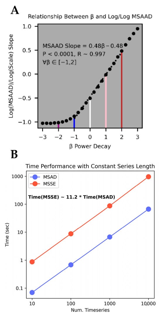
Figure 3.
(A). The slopes of the MSAAD curves from the log/log transformations plotted against the power decay constants for various noise realizations. Violet, blue, white, pink, and brown noise are highlighted as vertical lines with their colors. (B). Comparison of run times between MSAAD and MSSE for multiple iterations/sizes of data.
3.3. MSAAD of Distal Body Temperature Separates Individuals with a Diabetes Diagnosis from Individuals with No Reported Diagnoses
After analyzing the MSAAD and MSSE curves generated from idealized noise realizations, we evaluated the performance of each in identifying differences in signal complexity in real world samples of physiological data. We used data from the TemPredict Study [51], which included physiological data from 63,153 participants measured by the Oura Ring Gen2 (Oura Health Oy, Oulu, Finland) and paired survey data on participants’ health conditions (see Section 2). We first selected participants between the ages of 45 and 65 who reported having been diagnosed with diabetes (DM Dx), resulting in 328 males and 145 females. We then selected a sex-matched and age-matched comparison group of participants who reported having none of the listed medical conditions from the survey and who also indicated that they took no medications (No-DM Dx).
Statistically significant differences in MSAAD complexity curves were observed between DM Dx and No-DM Dx groups when measuring from both awake and asleep distal skin temperature (Figure 4 Rows 1 and 2). Both male and female No-DM Dx groups have significantly elevated daily MSAAD curves compared to their DM Dx counterparts (male: p < 0.001, Cohen’s d = 0.48; female: p < 0.001, Cohen’s d = 1.02) (Figure 4, Row 1). There are also statistically significant differences in daily MSAAD curves between No-DM Dx males and females (p < 0.001, Cohen’s d = −0.67). No significant difference was found in daily MSAAD curves between DM Dx males and females. The same significant relationships were found when using the nightly distal skin temperature; however, the directions of the effects were reversed (Figure 4, Row 2). Both No-DM Dx males and females had significantly lower nightly MSAAD curves compared to their DM Dx counterparts (males: p < 0.001, Cohen’s d = −0.56; females: p < 0.001, Cohen’s d = −0.73). The direction of the effect between males and females in the No-DM Dx group was reversed as well (p < 0.001, Cohen’s d: 0.15).
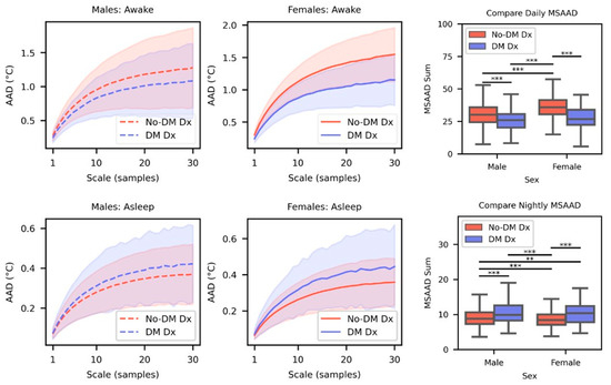
Figure 4.
Top Row. Mean MSAAD complexity curves for males (left) and females (center) for DM Dx and No-DM Dx cohorts when they were awake. The shaded area indicates the standard deviation. Comparisons are made between the sum of the curves for each cohort (right). Bottom Row. Same visualizations and comparisons as the top row but with temperature data sampled during sleep. (** p < 0.01, *** p < 0.001).
3.4. Comparisons of MSAAD Separating No-DM Dx vs. DM Dx Groups Versus MSSE and MS-KFD
The MS-KFD curves were similar in shape to the MSAAD curves (Figure A1); however, there were inconsistent effects in the DM Dx and No-DM Dx. For MS-KFD on asleep data, differences were only statistically significant when comparing No-DM Dx males to No-DM Dx females. For MS-KFD on awake data, there was a statistically significant effect between DM Dx and No-DM Dx males; however, no such effect was found in females.
The MSSE algorithm was sensitive to the number of samples, or the coarse-graining scale, used. As the scale increased, the algorithm returned more infeasible or missing values following a sigmoidal curve (Figure A2). For the daily data, the final scale of 30 samples returned roughly a 0.33 proportion of infeasible values in the sample; for the nightly data, the same scale returned a 0.99 proportion of infeasible values. The only statistically significant difference was found between No-DM Dx males and DM Dx males (p < 0.05, Cohen’s d: 0.39). A summary of median runtimes and separation of DM Dx and No-DM Dx cohorts with different state-of-the-art (SOTA) algorithms and MSAAD is summarized in Table 1.

Table 1.
Run time and distribution separability performance of MSAAD compared to other state-of-the-art (SOTA) algorithms. Best performing metrics for each column are bolded.
In summary, analysis with MSAAD revealed statistically significant differences between DM Dx and No-DM Dx females and males, while not being sensitive to increasing coursing scales. MS-KFD was unable to find consistent effects in both males and females. MSSE found no meaningful within-sex differences between DM Dx and No-DM Dx groups and was also negatively impacted by increasing coarse-graining scales.
Since levels of physical activity can affect skin temperature, we evaluated if the statistically significant effects found between No-DM Dx and DM Dx groups’ MSAAD estimates were maintained when incorporating metabolic equivalents (METs) and the Oura Ring’s estimate of activity. Using multilinear regression, we observe statistically significant coefficients for the group variable (No-DM Dx Vs. DM Dx) when accounting for awake/asleep state and sex (Table 2). The reference group is No-DM Dx, therefore positive or negative group coefficients indicate the No-DM Dx group has higher or lower mean MSAAD sums, respectively (reflective of Figure 3’s results). There are also statistically significant effects of MET and MSAAD intercepts in all models except for Male Asleep.
Table 2.
Multilinear regression coefficients and significance when identifying group effects in MSAAD.
3.5. MSAAD of Distal Body Temperature Highlights Differences in Reported Sex and Age
After quantifying the performance differences between MSAAD and MSSE when applied to the same set of temperature data to separate a binary variable (DM Dx vs. No-DM Dx), we used the TemPredict data to deploy MSAAD to larger temperature time series that have complexity that may be affected by a continuous variable (age).
Both females and males had greater distal body temperature MSAAD as a function of scale up to about 480 min, after which the MSAAD curve steeply decreased with the exception of a slight increase after a period of roughly one day (1440 min) (Figure 5A). Similarly to the males and females not reporting a DM Dx (reported above), there was once again an effect of sex on the mean complexities of both curves, independent of age (p < 0.001 in all comparisons, see Figure A4). We then investigated whether there were effects across the age groups at different coarse-graining scales. Both males and females had lower MSAAD as age increased, but the effect size (as measured by Spearman’s ρ) was heterogenous both between sexes and at certain coarse graining scales (Figure 5B). Correlations did not reach statistical significance or were of negligible size for coarse graining scales greater than 15 min and less than around 70 min for females. Comparing these correlations, where statistically significant, the association between age and AAD was stronger for men at coarse graining scales bin times less than 30 min. Stronger effects were found for females for bin times larger than 80 min.
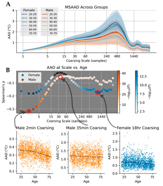
Figure 5.
(A). MSAAD curves of females (blues) and males (oranges) in different age tranches. Younger and older are darker and lighter hues, respectively. Mean of each curve is represented as solid lines, with standard deviation of group in shaded regions. (B). Scatterplot of Spearman’s when against coarsing scale when correlating the AAD values at each scale to continuous values of age. Negative values indicate a decrease in AAD at that scale at greater ages.
4. Discussion
Here, we created a multiscale version of Line Length, MSAAD, and evaluated its performance by identifying differences in cohorts with differing diabetes diagnoses, sexes, and ages using longitudinal, high-temporal-resolution human temperature data. We demonstrated that MSAAD is more stable and more computationally efficient than other conceptually similar analyses, and that it was able to detect novel biological patterns not detected by the standard techniques to which it was compared. We compared MSAAD with MSSE, a commonly used and powerful information theoretic analysis of physiological time series. Using 100 randomly generated synthetic processes, we showed that MSAAD has lower variance than MSSE at all scales for 0 ≤ β ≤ 2 and had a lesser rate of variance increase as scale increased. MSSE has been used as a form of time series digital biomarker [50,56,57]. Thus, to validate the more stable MSAAD as potentially useful in biological analyses, we conducted a number of comparisons to see if MSAAD revealed expected differences between cohorts, and if so, whether it did so with greater fidelity than the existing methods of MSSE and MS-KFD. We processed distal skin temperature data with MSAAD from men and women with and without self-reported DM Dx. We found that MSAAD curves revealed significant differences in males and females reporting either absence or presence of DM Dx, whereas MS-KFD and MSSE were unable to do so. Using MSAAD, we identified differences in distal skin temperature complexity across multiple age cohorts, and further highlight the importance of the multi-scale approach by showing that the effect of age is heterogenous across multiple temporal scales. While the process of aging impacts both females and males, it is not necessarily the case that age will lead to the same effect in distal temperature perturbations in both sexes. Sexual dimorphism in biological aging can be found in several processes such as mitochondrial function, inflammatory and immunological markers, and metabolism [58]. Since thermoregulation is affected by the processes that are in turn also affected by sexual dimorphism [59,60,61], the heterogeneous effects of age between sexes may manifest as a phenotypic change in measured distal skin temperature. These comparisons consistently confirmed that MSAAD was useful in finding differences in groups where biological differences were expected, both more consistently and with greater computational efficiency than the comparison methods.
Although the relationship between log(MSAAD)-log(Scale) slope is only linear for a subset of β values, those β values are also those that have been found in multiple biological and physiological systems, namely pink noise [62,63]. Pink noise found in physiological systems has been hypothesized to represent the stability of many interacting components, and its drift toward more white or brown noise has been associated with changes in such processes [64,65,66]. One reason we used diabetes and different age groups as test cases for MSAAD in this work was that prior work had used these same conditions to elucidate complexity changes in physiological signals [56,67].
It may seem counterintuitive that the direction of the effect of diabetes on both females and males is reversed depending on whether distal temperature is sampled when awake or asleep. However, it is important to consider the different states and covariates that are likely to affect the physiological data. Distal skin temperature changes driven by core temperature derive from blood heat radiating through capillaries in the skin [68], and so can change in response to a range of stimuli that affect capillary dilation, like ambient temperature, wind, and physical activity [69,70,71,72]. It is possible that the lower MSAAD during waking hours is associated with lower activity levels in the cohort with reported DM Dx. Alternatively, the higher MSAAD values in the DM Dx cohort during sleep could be associated with sleep disturbances that are known to impact individuals with diabetes [73,74], which may lead to more occurrences of wakefulness during the night, which would cause larger fluctuations in distal temperature. Interestingly, we still observed statistically significant differences in MSAAD between the No-DM Dx and DM Dx groups even when accounting for MET, the estimates of activity. This leads us to believe that there are perhaps non-linear relationships between physical activity and distal skin temperature, or that the fluctuations in temperature that MSAAD captures are indicative of underlying differences in thermoregulation. These larger fluctuations are likely also the reason why KFD does not separate cohorts as well as MSAAD. The KFD algorithm (Equation (A1)) is dependent on the point that creates the maximum distance to the first point, d. Because of this, external perturbations (e.g., waking up during the night, activity that affects distal temperature) can create large values for d, which are not actually related to the underlying temperature process itself but rather the effect that an external variable has on changes in temperature. As a result, the KFD algorithm is more sensitive to brief, large perturbations than the MSAAD algorithm, which is less affected by such perturbations due to its incorporation of averaging, which adds a smoothing effect. MSSE may not perform as well in separating time series of varying multi-scale complexity due to the fixed “tolerance” parameter, r, that sets a threshold for how far a comparison sequence can be to another sequence to be considered “close enough”. The fewer “close” matches there are in a time series, the more complex the signal is proposed to be. The r parameter is often based on the empirical global variance of the entire time series in question. Since skin temperature is a continuous signal that can be highly autocorrelated (the next sample is likely to be very close to the previous signal given no other external perturbations) but can have high global variance due to changes in ambient temperature or skin perfusion, the global variance may not be an appropriate value to use for comparisons between sequences. Therefore, the MSSE algorithm is likely less sensitive to higher frequency, low amplitude fluctuations.
At a higher level, the conceptual differences between the MSAAD, MSSE, and MS-KFD algorithms are related to how they individually approach the concept of irregularity or fluctuations. In MSSE, any subsequence of the time series is considered regular as long as an additional sample after the subsequence is within the tolerance. As such, any smaller fluctuations in the signal that are lower than the tolerance would still return a regular subsequence. Alternatively, MS-KFD is concerned with the fluctuations of a signal, but substantially affected by the largest distance between any pair of points in the entire signal. As such, estimates of complexity in signals with large perturbations from external factors (such as skin temperature being affected by external factors) from KFD are likely to be affected by the noise incurred by the largest possible deviation. The reasons for MSAAD outperforming both MSSE and MS-KFD is likely that it calculates a mean statistic on the distribution of fluctuations in the signal. This means that it does not smooth over smaller fluctuations like MSSE, and it is not as affected by singular large perturbations like MS-KFD.
We then showed that MSAAD is sensitive to distal skin temperature differences in cohorts defined by sex and age. More specifically, we show that there are differing effects of age on complexity that are both sex-dependent and scale-dependent. While prior work has identified a decrease in thermoregulatory complexity in aging cohorts with fewer individuals, to our knowledge we are the first to identify that longer timescales of fluctuation of distal temperature complexity are more affected by age in females, and that shorter timescales are more affected by age in males. These differences are identified with no assumptions made about the underlying process of the time series in question; that is, there are no parameters in the MSAAD computation other than coarse-graining scales.
Detrended fluctuation analysis (DFA) as well as information theoretic measures, such as sample entropy, can be used to estimate the complexity of a signal. However, each makes assumptions about the underlying structure of the data. For methods derived from DFA, the detrending can be any function fit to the data in a window of time [75]. While the choice of linear detrending is most common, it is not necessarily chosen based on a priori knowledge of the time series process. For methods derived from information theoretic measures, up to 3 parameters can be chosen depending on which specific entropy measurement is used: an embedding dimension (how many samples are used for a single computation), a delay (what is the quantity of time steps between samples that determine the addition of an additional embedding dimension), and a tolerance (what is the radius around samples in state-space that form an acceptable neighborhood). While there are strengths and limitations for using any estimate of complexity, we note that non-parametric choices presented by MSAAD may be preferable for data mining purposes since multiple cohorts may be annotated in a database, and the “ideal” choice of parameters that accounts for their potential heterogeneity cannot be known a priori.
While MSAAD was a strong separator of DM Dx and No-DM Dx, age, and sex in this work, we would like to highlight some limitations in the utilization of this algorithm in new contexts. For one, all skin temperature signals were approximated with the same class of thermistors used in the manufacturing of the wearable device. There are many devices that can estimate skin temperature, and their observation noise may be different than the observation noise of the device in this work. At higher frequencies, fluctuations are more likely to represent observation noise and not process noise. Secondly, MSAAD can be challenging for interpretation given that it highlights aperiodic fluctuations, therefore the presence of a dominant scale of fluctuation is not representative of a stationary, structural effect. Because of this, MSAAD is ideal for non-periodic fluctuating data; however, it is likely less useful for time series in which there exist strong temporal structure (i.e., a Fourier series). Despite these limitations, we believe that MSAAD is a useful parameterization of fluctuations in physiological time series and hope that future analyses can evaluate its clinical usefulness as well as how well it aids in improving performance of downstream algorithms that utilize it.
5. Conclusions
Physiological signals are affected by rhythms (both endogenous and exogenous), physical activity, health conditions, and stress levels. It is only in the past decade that vast amounts of high-temporal-resolution physiological data have been sampled from individuals for extended periods of time, and even more recently that these data could be used as tools to classify acute and chronic conditions. Given the size and depth of these datasets, we propose that MSAAD is a scalable, interpretable time series feature that is capable of identifying meaningful differences in physiological time series data without making assumptions of underlying process models or responses to perturbations.
Author Contributions
Conceptualization, J.H.B.; methodology, J.H.B.; software, J.H.B.; validation, J.H.B., W.H., S.D., A.E.M. and B.L.S.; formal analysis, J.H.B.; investigation, J.H.B.; resources, J.H.B., A.E.M. and B.L.S.; data curation, J.H.B.; writing—original draft preparation, J.H.B.; writing—review and editing, J.H.B., W.H., S.D., A.E.M. and B.L.S.; visualization, J.H.B.; supervision, A.E.M. and B.L.S.; project administration, A.E.M. and B.L.S.; funding acquisition, A.E.M. and B.L.S. All authors have read and agreed to the published version of the manuscript.
Funding
This effort was funded under MTEC solicitation MTEC-20-12-Diagnostics-023 and the USAMRDC under the Department of Defense (#MTEC-20-12-COVID19-D.-023). The #StartSmall foundation (#7029991) and Oura Health Oy (#134650) also provided funding for this work. The views expressed in this presentation are those of the author(s) and do not necessarily reflect the official policy of the Department of Defense, or the U.S. Government.
Institutional Review Board Statement
The University of California San Francisco (UCSF) Institutional Review Board (IRB, IRB# 20-30408) and the U.S. Department of Defense (DOD) Human Research Protections Office (HRPO, HRPO# E01877.1a) approved of all study activities, and all research was performed in accordance with relevant guidelines and regulations and the Declaration of Helsinki.
Informed Consent Statement
All participants provided informed electronic consent. We did not compensate participants for participation.
Data Availability Statement
Oura’s data use policy does not permit us to make wearable device data (collected via the Oura Ring) available to third parties. We can make self-report data available; please contact Ashley E. Mason and Benjamin L. Smarr to obtain an application to obtain these data.
Conflicts of Interest
A.E.M. has received remuneration for consulting work from Ouraring Inc. but declares no non-financial competing interests. B.L.S. has received remuneration for consulting work from, and has a financial interest in, Ouraring Inc. but declares no other non-financial competing interests. A.E.M., PhD, and B.L.S., PhD, are listed as co-inventors on patent applications as follows: 17/357,922, filed 24 June 2021, entitled “ILLNESS DETECTION BASED ON TEMPERATURE DATA,” status is pending; PCT/US21/39260, filed 25 June 2021, entitled “ILLNESS DETECTION BASED ON TEMPERATURE DATA,” status is expired; and 17/357,930, filed 24 June 2021, entitled “HEALTH MONITORING PLATFORM FOR ILLNESS DETECTION,” status is pending. These were all filed as of July 2021 by Oura Health Oy on behalf of UCSD. All applications cover the use of wearable device data to detect illness onset.
Abbreviations
The following abbreviations are used in this manuscript:
| (MS)AAD | (Multiscale) Average Absolute Difference |
| (MS)SE | (Multiscale) Sample Entropy |
| (MS)PE | (Multiscale) Permutation Entropy |
| (MS-)KFD | (Multiscale) Katz Fractal Dimension |
| DFA | Detrended Fluctuation Analysis |
| Dx | Diagnosis |
Appendix A

Figure A1.
Top Row. Mean MS-KFD complexity curves for males (left) and females (center) for DM Dx and No-DM Dx cohorts when they were awake. The shaded area indicates the standard deviation. Comparisons are made between the sum of the curves for each cohort (right). Bottom Row. Same visualizations and comparisons as the top row but with temperature data sampled during sleep. (** p < 0.01, *** p < 0.001).

Figure A2.
Top Row. Mean MSSE complexity curves for males (left) and females (center) for DM Dx and No-DM Dx cohorts when they were awake. The shaded area indicates the standard deviation. Comparisons are made between the sum of the curves for each cohort (right). Bottom Row. Same visualizations and comparisons as the top row but with temperature data sampled during sleep. (* p < 0.05).

Figure A3.
p-values of negative control distribution (blue shaded curve) against experimental significance found between the MSAAD curves across the No-DM Dx and DM Dx cohorts.

Figure A4.
Mann–Whitney U tests between female and male groups based on their MSAAD curve sums across different ages (*** p < 0.001).
is the line-length of a curve (sum of the absolute differences between points) and is the value that creates the maximum distance to the first value.
References
- Niknejad, N.; Ismail, W.B.; Mardani, A.; Liao, H.; Ghani, I. A comprehensive overview of smart wearables: The state of the art literature, recent advances, and future challenges. Eng. Appl. Artif. Intell. 2020, 90, 103529. [Google Scholar] [CrossRef]
- Gao, S.; Zhang, X.; Peng, S. Understanding the Adoption of Smart Wearable Devices to Assist Healthcare in China; Springer: Berlin/Heidelberg, Germany, 2016; pp. 280–291. [Google Scholar]
- Grym, K.; Niela-Vilén, H.; Ekholm, E.; Hamari, L.; Azimi, I.; Rahmani, A.; Liljeberg, P.; Löyttyniemi, E.; Axelin, A. Feasibility of smart wristbands for continuous monitoring during pregnancy and one month after birth. BMC Pregnancy Childbirth 2019, 19, 34. [Google Scholar] [CrossRef]
- Aliverti, A. Wearable technology: Role in respiratory health and disease. Breathe 2017, 13, e27–e36. [Google Scholar] [CrossRef] [PubMed]
- Li, J.; Ma, Q.; Chan, A.H.; Man, S. Health monitoring through wearable technologies for older adults: Smart wearables acceptance model. Appl. Ergon. 2019, 75, 162–169. [Google Scholar] [CrossRef]
- Babu, M.; Lautman, Z.; Lin, X.; Sobota, M.H.B.; Snyder, M.P. Wearable Devices: Implications for Precision Medicine and the Future of Health Care. Annu. Rev. Med. 2024, 75, 401–415. [Google Scholar] [CrossRef]
- Burks, J.H.; Bruce, L.K.; Kasl, P.; Soltani, S.; Viswanath, V.; Hartogensis, W.; Dilchert, S.; Hecht, F.M.; Dasgupta, S.; Altintas, I.; et al. General feature selection technique supporting sex-debiasing in chronic illness algorithms validated using wearable device data. npj Women’s Health 2024, 2, 37. [Google Scholar] [CrossRef]
- Burks, J.H.; Joe, L.; Kanjaria, K.; Monsivais, C.; O’laughlin, K.; Smarr, B.L. Chronobiologically-informed features from CGM data provide unique information for XGBoost prediction of longer-term glycemic dysregulation in 8,000 individuals with type-2 diabetes. PLoS Digit. Health 2025, 4, e0000815. [Google Scholar] [CrossRef]
- Mattison, G.; Canfell, O.; Forrester, D.; Dobbins, C.; Smith, D.; Töyräs, J.; Sullivan, C. The Influence of Wearables on Health Care Outcomes in Chronic Disease: Systematic Review. J. Med. Internet Res. 2022, 24, e36690. [Google Scholar] [CrossRef] [PubMed]
- Dunn, J.; Runge, R.; Snyder, M. Wearables and the medical revolution. Pers. Med. 2018, 15, 429–448. [Google Scholar] [CrossRef] [PubMed]
- Hamilton, J.D. Time Series Analysis; Princeton University Press: Princeton, NJ, USA, 2020; ISBN 0-691-21863-3. [Google Scholar]
- Klein, J.L. Statistical Visions in Time: A History of Time Series Analysis, 1662–1938; Cambridge University Press: Cambridge, UK, 1997; ISBN 0-521-42046-6. [Google Scholar]
- Attinger, E.; Anne, A.; McDonald, D. Use of Fourier series for the analysis of biological systems. Biophys. J. 1966, 6, 291–304. [Google Scholar] [CrossRef]
- Kohlmorgen, J.; Müller, K.-R.; Rittweger, J.; Pawelzik, K. Identification of nonstationary dynamics in physiological recordings. Biol. Cybern. 2000, 83, 73–84. [Google Scholar] [CrossRef]
- Mayer-Kress, G. Localized measures for nonstationary time-series of physiological data. Integr. Physiol. Behav. Sci. 1994, 29, 205–210. [Google Scholar] [CrossRef] [PubMed]
- Tang, L.; Lv, H.; Yang, F.; Yu, L. Complexity testing techniques for time series data: A comprehensive literature review. Chaos Solitons Fractals 2015, 81, 117–135. [Google Scholar] [CrossRef]
- Song, C.; Havlin, S.; Makse, H.A. Self-similarity of complex networks. Nature 2005, 433, 392–395. [Google Scholar] [CrossRef] [PubMed]
- Barkoulas, J.T.; Baum, C.F. Long-term dependence in stock returns. Econ. Lett. 1996, 53, 253–259. [Google Scholar] [CrossRef]
- Lipsitz, L.A.; Goldberger, A.L. Loss of ’complexity’ and aging: Potential applications of fractals and chaos theory to senescence. JAMA 1992, 267, 1806–1809. [Google Scholar] [CrossRef]
- Stam, C.J. Nonlinear dynamical analysis of EEG and MEG: Review of an emerging field. Clin. Neurophysiol. 2005, 116, 2266–2301. [Google Scholar] [CrossRef]
- Sharma, V. Deterministic chaos and fractal complexity in the dynamics of cardiovascular behavior: Perspectives on a new frontier. Open Cardiovasc. Med. J. 2009, 3, 110. [Google Scholar] [CrossRef]
- Powell, G.; Percival, I. A spectral entropy method for distinguishing regular and irregular motion of Hamiltonian systems. J. Phys. Math. Gen. 1979, 12, 2053. [Google Scholar] [CrossRef]
- Richman, J.S.; Moorman, J.R. Physiological time-series analysis using approximate entropy and sample entropy. Am. J. Physiol. Heart Circ. Physiol. 2000, 278, H2039–H2049. [Google Scholar] [CrossRef]
- Rosso, O.A.; Blanco, S.; Yordanova, J.; Kolev, V.; Figliola, A.; Schürmann, M.; Başar, E. Wavelet entropy: A new tool for analysis of short duration brain electrical signals. J. Neurosci. Methods 2001, 105, 65–75. [Google Scholar] [CrossRef] [PubMed]
- Bandt, C.; Pompe, B. Permutation entropy: A natural complexity measure for time series. Phys. Rev. Lett. 2002, 88, 174102. [Google Scholar] [CrossRef] [PubMed]
- Bryce, R.M.; Sprague, K.B. Revisiting detrended fluctuation analysis. Sci. Rep. 2012, 2, 315. [Google Scholar] [CrossRef]
- Lv, J.-H.; Lu, J.-A.; Chen, S. Analysis and Application of Chaotic Time Series; Press of Wuhan University: Wuhan, China, 2002. [Google Scholar]
- Lake, D.E.; Richman, J.S.; Griffin, M.P.; Moorman, J.R. Sample entropy analysis of neonatal heart rate variability. Am. J. Physiol.-Regul. Integr. Comp. Physiol. 2002, 283, R789–R797. [Google Scholar] [CrossRef] [PubMed]
- Alcaraz, R.; Rieta, J. A novel application of sample entropy to the electrocardiogram of atrial fibrillation. Nonlinear Anal. Real World Appl. 2010, 11, 1026–1035. [Google Scholar] [CrossRef]
- Bian, C.; Qin, C.; Ma, Q.D.; Shen, Q. Modified permutation-entropy analysis of heartbeat dynamics. Phys. Rev. E 2012, 85, 21906. [Google Scholar] [CrossRef]
- Deffeyes, J.E.; Harbourne, R.T.; Stuberg, W.A.; Stergiou, N. Approximate entropy used to assess sitting postural sway of infants with developmental delay. Infant Behav. Dev. 2011, 34, 81–99. [Google Scholar] [CrossRef]
- Pincus, S.M. Approximate entropy as a measure of system complexity. Proc. Natl. Acad. Sci. USA 1991, 88, 2297–2301. [Google Scholar] [CrossRef]
- Galaska, R.; Makowiec, D.; Dudkowska, A.; Koprowski, A.; Chlebus, K.; Wdowczyk-Szulc, J.; Rynkiewicz, A. Comparison of wavelet transform modulus maxima and multifractal detrended fluctuation analysis of heart rate in patients with systolic dysfunction of left ventricle. Ann. Noninvasive Electrocardiol. 2008, 13, 155–164. [Google Scholar] [CrossRef]
- Humeau, A.; Buard, B.; Mahé, G.; Chapeau-Blondeau, F.; Rousseau, D.; Abraham, P. Multifractal analysis of heart rate variability and laser Doppler flowmetry fluctuations: Comparison of results from different numerical methods. Phys. Med. Biol. 2010, 55, 6279. [Google Scholar] [CrossRef]
- Dick, O.E. Multifractal analysis of the psychorelaxation efficiency for the healthy and pathological human brain. Chaotic Model Simul 2012, 1, 219–227. [Google Scholar]
- Mercy Cleetus, H.M.; Singh, D. Multifractal application on electrocardiogram. J. Med. Eng. Technol. 2014, 38, 55–61. [Google Scholar] [CrossRef]
- Babloyantz, A.; Salazar, J.; Nicolis, C. Evidence of chaotic dynamics of brain activity during the sleep cycle. Phys. Lett. A 1985, 111, 152–156. [Google Scholar] [CrossRef]
- Thomasson, N.; Hoeppner, T.J.; Webber, C.L., Jr.; Zbilut, J.P. Recurrence quantification in epileptic EEGs. Phys. Lett. A 2001, 279, 94–101. [Google Scholar] [CrossRef]
- Yılmaz, D.; Güler, N.F. Analysis of the Doppler signals using largest Lyapunov exponent and correlation dimension in healthy and stenosed internal carotid artery patients. Digit. Signal Process. 2010, 20, 401–409. [Google Scholar] [CrossRef]
- Übeyli, E.D. Lyapunov exponents/probabilistic neural networks for analysis of EEG signals. Expert Syst. Appl. 2010, 37, 985–992. [Google Scholar] [CrossRef]
- Canali, S.; Schiaffonati, V.; Aliverti, A. Challenges and recommendations for wearable devices in digital health: Data quality, interoperability, health equity, fairness. PLoS Digit. Health 2022, 1, e0000104. [Google Scholar] [CrossRef] [PubMed]
- Schlink, U.; Ueberham, M. Perspectives of Individual-Worn Sensors Assessing Personal Environmental Exposure. Engineering 2021, 7, 285–289. [Google Scholar] [CrossRef]
- Taylor, K.I.; Staunton, H.; Lipsmeier, F.; Nobbs, D.; Lindemann, M. Outcome measures based on digital health technology sensor data: Data- and patient-centric approaches. npj Digit. Med. 2020, 3, 97. [Google Scholar] [CrossRef]
- Elsenbruch, S.; Wang, Z.; Orr, W.C.; Chen, J. Time-frequency analysis of heart rate variability using short-time Fourier analysis. Physiol. Meas. 2000, 21, 229. [Google Scholar] [CrossRef]
- Silva, B.M.C.; Rodrigues, J.J.P.C.; de la Torre Díez, I.; López-Coronado, M.; Saleem, K. Mobile-health: A review of current state in 2015. J. Biomed. Inform. 2015, 56, 265–272. [Google Scholar] [CrossRef] [PubMed]
- Steinhubl, S.R.; Muse, E.D.; Topol, E.J. The emerging field of mobile health. Sci. Transl. Med. 2015, 7, 283rv3. [Google Scholar] [CrossRef]
- Weinstein, R.S.; Lopez, A.M.; Joseph, B.A.; Erps, K.A.; Holcomb, M.; Barker, G.P.; Krupinski, E.A. Telemedicine, Telehealth, and Mobile Health Applications That Work: Opportunities and Barriers. Am. J. Med. 2014, 127, 183–187. [Google Scholar] [CrossRef]
- Katz, M.J. Fractals and the analysis of waveforms. Comput. Biol. Med. 1988, 18, 145–156. [Google Scholar] [CrossRef]
- Costa, M.; Goldberger, A.L.; Peng, C.-K. Multiscale Entropy Analysis (MSE). A Tutor MSE. 2000. Available online: https://www.physionet.org/files/mse/1.0/tutorial/tutorial.pdf (accessed on 25 January 2025).
- Costa, M.; Goldberger, A.L.; Peng, C.-K. Multiscale entropy analysis of complex physiologic time series. Phys. Rev. Lett. 2002, 89, 68102. [Google Scholar] [CrossRef] [PubMed]
- Mason, A.E.; Hecht, F.M.; Davis, S.K.; Natale, J.L.; Hartogensis, W.; Damaso, N.; Claypool, K.T.; Dilchert, S.; Dasgupta, S.; Purawat, S. Detection of COVID-19 using multimodal data from a wearable device: Results from the first TemPredict Study. Sci. Rep. 2022, 12, 3463. [Google Scholar]
- Malakhatka, E.; Osman, O.; Lundqvist, P. Monitoring and Predicting Occupant’s Sleep Quality by Using Wearable Device OURA Ring and Smart Building Sensors Data (Living Laboratory Case Study). Buildings 2021, 11, 459. [Google Scholar] [CrossRef]
- Kenny, G.P.; Sigal, R.J.; McGinn, R. Body temperature regulation in diabetes. Temp. Multidiscip. Biomed. J. 2016, 3, 119–145. [Google Scholar] [CrossRef]
- Arabi, P.M.; Joshi, G.; Lohith, S.; Mubashir, M.; Pallavi, P.Y.; Surabhi, M. Early Diagnosis of Diabetic Vasculopathy by Thermo-Regulatory Vascular Impairment. In Proceedings of the 2020 5th International Conference on Communication and Electronics Systems (ICCES), Coimbatore, India, 10–12 June 2020; pp. 1368–1373. [Google Scholar]
- Rutkove, S.B.; Veves, A.; Mitsa, T.; Nie, R.; Fogerson, P.M.; Garmirian, L.P.; Nardin, R.A. Impaired Distal Thermoregulation in Diabetes and Diabetic Polyneuropathy. Diabetes Care 2009, 32, 671–676. [Google Scholar] [CrossRef]
- Costa, M.D.; Henriques, T.; Munshi, M.N.; Segal, A.R.; Goldberger, A.L. Dynamical glucometry: Use of multiscale entropy analysis in diabetes. Chaos 2014, 24, 33139. [Google Scholar] [CrossRef] [PubMed]
- Kosciessa, J.Q.; Kloosterman, N.A.; Garrett, D.D. Standard multiscale entropy reflects neural dynamics at mismatched temporal scales: What’s signal irregularity got to do with it? PLoS Comput. Biol. 2020, 16, e1007885. [Google Scholar] [CrossRef] [PubMed]
- Hägg, S.; Jylhävä, J. Sex differences in biological aging with a focus on human studies. eLife 2021, 10, e63425. [Google Scholar] [CrossRef] [PubMed]
- Chan, S.L.; Wei, Z.; Chigurupati, S.; Tu, W. Compromised respiratory adaptation and thermoregulation in aging and age-related diseases. Thermodyn. Ageing 2010, 9, 20–40. [Google Scholar] [CrossRef]
- Irwin, M.R. Sleep disruption induces activation of inflammation and heightens risk for infectious disease: Role of impairments in thermoregulation and elevated ambient temperature. Temperature 2023, 10, 198–234. [Google Scholar] [CrossRef] [PubMed]
- Haskell, E.H.; Palca, J.W.; Walker, J.M.; Berger, R.J.; Heller, H.C. Metabolism and thermoregulation during stages of sleep in humans exposed to heat and cold. J. Appl. Physiol. 1981, 51, 948–954. [Google Scholar] [CrossRef]
- Hausdorff, J.M.; Peng, C.-K. Multiscaled randomness: A possible source of 1/f noise in biology. Phys. Rev. E 1996, 54, 2154. [Google Scholar] [CrossRef]
- Musha, T.; Yamamoto, M. 1/f Fluctuations in Biological Systems; IEEE: New York, NY, USA, 1997; Volume 6, pp. 2692–2697. [Google Scholar]
- Sejdić, E.; Lipsitz, L.A. Necessity of noise in physiology and medicine. Comput. Methods Programs Biomed. 2013, 111, 459–470. [Google Scholar] [CrossRef]
- Pilgram, B.; Kaplan, D.T. Nonstationarity and 1/f noise characteristics in heart rate. Am. J. Physiol.-Regul. Integr. Comp. Physiol. 1999, 276, R1–R9. [Google Scholar] [CrossRef]
- Ward, L.M.; Greenwood, P.E. 1/f noise. Scholarpedia 2007, 2, 1537. [Google Scholar] [CrossRef]
- Tran, T.T.; Rolle, C.E.; Gazzaley, A.; Voytek, B. Linked Sources of Neural Noise Contribute to Age-related Cognitive Decline. J. Cogn. Neurosci. 2020, 32, 1813–1822. [Google Scholar] [CrossRef]
- Osilla, E.V.; Marsidi, J.L.; Shumway, K.R.; Sharma, S. Physiology, Temperature Regulation. In StatPearls; StatPearls Publishing: Treasure Island, FL, USA, 2024. [Google Scholar]
- Stoner, H.B.; Barker, P.; Riding, G.S.; Hazlehurst, D.E.; Taylor, L.; Marcuson, R.W. Relationships between skin temperature and perfusion in the arm and leg. Clin. Physiol. Oxf. Engl. 1991, 11, 27–40. [Google Scholar] [CrossRef]
- Romanovsky, A.A. Skin temperature: Its role in thermoregulation. Acta Physiol. Oxf. Engl. 2014, 210, 498–507. [Google Scholar] [CrossRef]
- LeBlanc, J.; Blais, B.; Barabé, B.; Côté, J. Effects of temperature and wind on facial temperature, heart rate, and sensation. J. Appl. Physiol. 1976, 40, 127–131. [Google Scholar] [CrossRef]
- Torii, M.; Yamasaki, M.; Sasaki, T.; Nakayama, H. Fall in skin temperature of exercising man. Br. J. Sports Med. 1992, 26, 29–32. [Google Scholar] [CrossRef] [PubMed]
- Surani, S.; Brito, V.; Surani, A.; Ghamande, S. Effect of diabetes mellitus on sleep quality. World J. Diabetes 2015, 6, 868–873. [Google Scholar] [CrossRef] [PubMed]
- Ogilvie, R.P.; Patel, S.R. The Epidemiology of Sleep and Diabetes. Curr. Diab. Rep. 2018, 18, 82. [Google Scholar] [CrossRef] [PubMed]
- Hu, K.; Ivanov, P.C.; Chen, Z.; Carpena, P.; Eugene Stanley, H. Effect of trends on detrended fluctuation analysis. Phys. Rev. E 2001, 64, 11114. [Google Scholar] [CrossRef]
Disclaimer/Publisher’s Note: The statements, opinions and data contained in all publications are solely those of the individual author(s) and contributor(s) and not of MDPI and/or the editor(s). MDPI and/or the editor(s) disclaim responsibility for any injury to people or property resulting from any ideas, methods, instructions or products referred to in the content. |
© 2025 by the authors. Licensee MDPI, Basel, Switzerland. This article is an open access article distributed under the terms and conditions of the Creative Commons Attribution (CC BY) license (https://creativecommons.org/licenses/by/4.0/).