Exploring the Frequency Domain Point Cloud Processing for Localisation Purposes in Arboreal Environments

Abstract

Point clouds from 3D sensors such as LiDAR are increasingly used in agriculture for tasks like crop characterisation, pest detection, and leaf area estimation. While traditional point cloud processing typically occurs in Cartesian space using methods such as principal component analysis (PCA), this paper introduces a novel frequency-domain approach for point cloud registration. The central idea is that point clouds can be transformed and analysed in the spectral domain, where key frequency components capture the most informative spatial structures. By selecting and registering only the dominant frequencies, our method achieves significant reductions in localisation error and computational complexity. We validate this approach using public datasets and compare it with standard Iterative Closest Point (ICP) techniques. Our method, which applies ICP only to points in selected frequency bands, reduces localisation error from 4.37 m to 1.22 m (MSE), an improvement of approximately 72%. These findings highlight the potential of frequency-domain analysis as a powerful and efficient tool for point cloud registration in agricultural and other GNSS-challenged environments.

1. Introduction

Accurate localisation in complex and unstructured environments—such as forests and other arboreal settings—is a critical enabler for a wide range of applications, including environmental monitoring, autonomous navigation, forestry management, and precision agriculture. Traditional GPS-based localisation methods often perform poorly under dense canopy cover or in GPS-denied environments, highlighting the need for alternative localisation strategies. Advances in LiDAR technology and point cloud processing have opened new avenues for achieving precise localisation in such challenging contexts, allowing robots and autonomous systems to operate more reliably and efficiently in natural environments.

Recent research has increasingly focused on improving localisation capabilities in these environments, particularly in forested areas. In [1], a topology-based method is proposed using Delaunay triangulation to match local point clouds to a global tree map, achieving an accuracy of 12 cm in forest operations. In [2], a point cloud transformation technique is introduced that enhances the visibility of tree instances in TLS data, enabling the use of topology-based methods in forest scenarios. In [3], a deep learning approach is developed for laser-based localisation in urban and natural environments, creating meaningful descriptors from 3D point clouds for loop closure detection. Previously, Tinchev et al. [4] presented the Natural Segmentation and Matching (NSM) algorithm, which extracts stable object-sized segments and key poses from point clouds, facilitating robust localisation in both urban and arboreal contexts. These contributions collectively demonstrate the growing capability of current methods to localise accurately in unstructured, natural environments.

Point cloud processing for localisation in arboreal environments is predominantly based on LiDAR technologies, with three-dimensional LiDAR being the most commonly used sensor in seven of the reviewed studies. While some researchers rely on standalone LiDAR systems, others explore sensor fusion strategies that integrate LiDAR with inertial navigation systems (INSs), cameras, and aerial imagery [5,6,7]. Notably, two-dimensional LiDAR solutions have also proven effective, especially in cost-sensitive applications [8,9] (and the references there in).

The range of processing methods spans from traditional geometric matching to cutting-edge deep learning techniques. Classical geometric approaches—such as the Modified Hausdorff Distance and Iterative Closest Point (ICP)—serve as foundational tools in several studies [10,11]. Simultaneous Localisation and Mapping (SLAM)-based methods have shown particular promise, with implementations including graph-SLAM and pose-graph SLAM [11,12]. More recent efforts have incorporated deep learning and semantic segmentation, which have improved robustness in dynamic and cluttered conditions [13].

These technologies have been tested across a wide variety of arboreal environments, with forest settings being the most frequently studied, appearing in seven publications. Other applications include dense forests, parklands, urban environments, and specialised contexts such as orchards and arboreal fruit farming [9,13]. This diversity in deployment settings underscores the adaptability and generalisability of point cloud-based localisation techniques.

Performance metrics and implementation results vary across studies. In [11], a systematic comparison analysis is presented about the accuracy of point cloud registration techniques when used in GNSS (global navigation satellite system)-denied environments.

Problem Statement

Point cloud registration techniques, as detailed in Section 2, process 3D data acquired from various sources such as LiDAR, RGB-D cameras, and other depth-sensing technologies. These techniques typically operate in Cartesian space to identify correspondences between two or more point clouds. Prior to establishing correspondences, registration pipelines often include preprocessing steps to eliminate outliers or irrelevant regions. For instance, in [14], the ground surface is manually removed to reduce processing complexity.

As the quality of the matching is intrinsically dependent on the alignment between the point clouds—see [8,9] and references therein—we propose an alternative approach to address this problem. Rather than working directly in Cartesian space, we transform the point cloud into the frequency domain. In this transformed space, we analyse the frequency responses to identify specific frequency bands that minimise the matching error and thus reduce the overall localisation error.

Once the optimal frequency bands are identified, points not belonging to these bands are automatically filtered out. The remaining points are then re-transformed back into Cartesian space, and the registration process is performed on this reduced dataset. Our hypothesis is based on the observation that in arboreal environments, points within the canopy typically exhibit higher variability in their frequency components, whereas ground points—often associated with planar structures—tend to display more consistent frequency characteristics. This insight motivates our exploration of frequency-domain filtering as a means to improve the robustness and accuracy of point cloud registration.

2. Point Cloud Registration

Registration techniques are generally categorised into two main types [15,16]: global and local. Global registration methods estimate the relative pose between point clouds without prior alignment, typically relying on geometric features or robust optimisation to compute an initial coarse transformation. This is then refined using local techniques. In contrast, local registration assumes an approximate initial pose and iteratively refines it, with methods such as Iterative Closest Point (ICP) and its variants minimising the distance between corresponding points across scans [17,18].

Accurate point cloud registration is essential for tasks such as map construction, sensor fusion, and tracking of objects or mobile platforms. However, challenges arise due to noise, outliers, dynamic elements, and partial overlaps between scans [19,20].

Point cloud registration plays a central role in robotic localisation systems. In GPS-denied or unreliable environments—such as orchards, forests, tunnels, or indoor areas—robots depend on onboard 3D LiDAR sensors to perceive their surroundings. These sensors produce dense point clouds that capture the geometry of the environment. By registering new scans to prior scans or prebuilt maps, the robot estimates its pose relative to known references. This capability is often embedded in SLAM (Simultaneous Localisation and Mapping) frameworks, supporting both localisation and map building. Widely used techniques include ICP and feature-based registration, while more recent systems incorporate semantic information or deep learning-based descriptors for increased robustness under diverse conditions. Consequently, point cloud registration is a foundational component of autonomous navigation, mapping, and decision-making in robotics.

Comprehensive surveys of registration methods and their application to robotic localisation are available in [8,9,11]. In this work, we use the ICP implementation from [9] as a baseline to validate our hypothesis: that frequency-domain filtering can significantly improve registration accuracy by focusing computation on the most informative spatial frequencies.

3. Point Cloud Frequency Domains

This section presents the mathematical concepts underpinning the analysis of point clouds in the frequency domain using graph-based techniques, with the aim of demonstrating how this domain provides valuable insights for point cloud registration. Specifically, we explore how the smoothness of signals defined on graphs can be quantified and how the Graph Fourier Transform (GFT) offers a principled framework for frequency analysis by drawing from both graph theory and signal processing.

We begin by introducing the concept of the Graph Fourier Transform and its application to signals defined on graph structures. This requires an understanding of how the eigenvalues and eigenvectors of the graph Laplacian form a spectral basis, analogous to the frequency components in the classical Fourier transform.

Next, we employ tools from discrete calculus to formalise the notion of smoothness on graphs, highlighting how the topology and connectivity of the underlying graph influence signal variation. This approach provides a systematic way to analyse signal fluctuations and frequency characteristics within point clouds while simultaneously offering structural insights into the graph representation of the data.

3.1. Point Cloud Graph Characterisation

Let us define a point cloud representation on an undirected, connected, weighted graph $\mathbf{G}=\{V,E,\mathbf{W}\}$, where V is the set of vertices representing point locations, E is the set of edges, and $\mathbf{W}$ is a symmetric weight matrix of size $N\times N$ (see [11] for further details). A thresholded Gaussian kernel weighting function is used to encode local geometric information; hence, the weight $W_{m,n}$ between vertices m and n is defined as

$${\mathbf{W}}_{m,n}=\left\{\begin{array}{cc}exp\left(-{\displaystyle \frac{\parallel x_m-x_n{\parallel }^2}{2{\sigma }^2}}\right),\hfill & \mathrm{if}\parallel x_m-x_n\parallel \le \tau \hfill \\ 0,\hfill & \mathrm{otherwise}\hfill \end{array}\right.$$

where $\sigma$ and $\tau$ are the spread parameter of the Gaussian kernel and the distance threshold for edge construction, respectively.

Assuming that the degree $d\left(m\right)$ of a vertex m is the sum of the weights of all edges incident to m, it can be expressed as $d\left(m\right)={\sum }_n{\mathbf{W}}_{m,n}$. The degree matrix $\mathbf{D}$ is then the diagonal matrix with elements $D_{m,m}=d\left(m\right)$. The unnormalised graph Laplacian is defined as $\mathbf{L}=\mathbf{D}-\mathbf{W}$. Thus, the graph Laplacian acts as a difference operator, which for any signal $\mathbf{f}\in {\mathbb{R}}^N$ satisfies

$$\left(\mathbf{L}f\right)\left(m\right)=\sum _{n\in N_m}{\mathbf{W}}_{m,n}·\left(f\left(m\right)-f\left(n\right)\right)$$

where $N_m$ is the set of vertices connected to vertex m. Since the graph Laplacian $\mathbf{L}$ is a real symmetric matrix, it admits a complete set of orthonormal eigenvectors ${\left\{{\mathbf{v}}_l\right\}}_{l=0,1,\dots ,N-1}$, associated with real, non-negative eigenvalues ${\left\{{\lambda }_l\right\}}_{l=0,1,\dots ,N-1}$. The eigen decomposition of the graph Laplacian is given by

$$\mathbf{L}{\mathbf{v}}_l={\lambda }_l{\mathbf{v}}_l$$

The eigenvalues of the graph Laplacian are ordered as $0={\lambda }_0<{\lambda }_1\le {\lambda }_2\le \dots \le {\lambda }_{N-1}:={\lambda }_{\max }$.

3.2. Graph Fourier Transform (GFT)

The classical Fourier transform, defined as

$$\widehat{f}\left(\xi \right):=〈f,e^{2\pi i\xi t}〉={\int }_{\mathbb{R}}f\left(t\right)e^{-2\pi i\xi t}dt$$

represents a function f as an expansion in terms of complex exponentials, which are the eigenfunctions of the one-dimensional Laplace operator:

$$-\Delta \left(e^{2\pi i\xi t}\right)=-{\displaystyle \frac{{\partial }^2}{\partial t^2}}{e}^{2\pi i\xi t}={\left(2\pi \xi \right)}^2{e}^{2\pi i\xi t}$$

Analogously, the Graph Fourier Transform (GFT) of a function $f\in {\mathbb{R}}^N$ defined on the vertices of a graph $\mathbf{G}$ is the expansion of f in terms of the eigenvectors of the graph Laplacian $\mathbf{L}$:

$$\widehat{f}\left({\lambda }_l\right):=〈f,{\mathbf{v}}_l〉=\sum _{m=1}^{N}f\left(m\right){\mathbf{v}}_l^{*}\left(m\right)$$

where ${\mathbf{v}}_l$ are the eigenvectors of $\mathbf{L}$ associated with eigenvalues ${\lambda }_l$. The inverse GFT is defined as

$$f\left(m\right)=\sum _{l=0}^{N-1}\widehat{f}\left({\lambda }_l\right){\mathbf{v}}_l\left(m\right)$$

In classical Fourier analysis, the eigenvalues ${\left(2\pi \xi \right)}^2$ represent frequency: lower values correspond to slowly oscillating components while higher values correspond to rapidly oscillating ones. Similarly, in the graph setting, the eigenvalues ${\lambda }_l$ of the Laplacian provide a notion of frequency. The eigenvector ${\mathbf{v}}_0$, associated with ${\lambda }_0=0$, is constant across the graph. Eigenvectors corresponding to low eigenvalues vary smoothly across adjacent nodes, while those corresponding to high eigenvalues oscillate more rapidly over the graph structure.

To deepen this understanding, we now consider the notion of signal smoothness on graphs and how it is influenced by the intrinsic topology of the graph. This requires the use of discrete calculus to formally quantify smoothness and variation.

3.3. Discrete Calculus and Signal Smoothness

In order to analyse signals on graphs, features such as smoothness must be considered in relation to the graph’s underlying structure. The mathematical tools required to work with signals defined in a discrete space are provided by the following discrete differential operators:

• Edge derivative,
• Graph gradient,
• Local variation.

To better understand the geometric significance of these operators, let us begin with a simple example: a row of points with a signal defined over them. If the distance between the points is constant, the discrete derivative (i.e., the difference between consecutive signal values) indicates how rapidly the signal changes:

$${\displaystyle \frac{\partial f}{\partial x_m}}\approx f\left(x_{m+1}\right)-f\left(x_m\right)$$

If this difference is small for all points, the signal is considered smooth.

For graphs, the concept is similar, but the points (vertices) are not arranged linearly and may have arbitrary connections (e.g., grids, trees, random graphs). The edge derivative of a signal f with respect to an edge $e=\left(m,n\right)$ at vertex m is defined as

$${\left.{\displaystyle \frac{\partial f}{\partial e}}\right|}_m:=\sqrt{W_{m,n}}\left[f\left(n\right)-f\left(m\right)\right]$$

where $W_{m,n}$ represents the weight of the edge connecting vertices m and n. The edge derivative quantifies the variation of the signal between two connected vertices.

The graph gradient is then a vector that collects all such derivatives for a given vertex m, defined as

$${\nabla }_m\mathbf{f}:=\left[{\left\{{\left.{\displaystyle \frac{\partial \mathbf{f}}{\partial e}}\right|}_m\right\}}_{e\in \epsilon ,\mathrm{s}.\mathrm{t}.e=\left(m,n\right)\mathrm{for}\mathrm{some}n\in \nu }\right]$$

The local variation quantifies how the signal changes around a single vertex. A small local variation indicates that the signal is smooth in the vicinity of vertex m, meaning that f takes similar values at m and its neighbors. It is defined as

$${∥{\nabla }_{m}f∥}_2={\left(\sum _{n\in N_m}{W}_{m,n}{\left[f\left(n\right)-f\left(m\right)\right]}^2\right)}^{{\displaystyle \frac{1}{2}}}$$

To extend this concept to the entire graph, the discrete p-Dirichlet form is used to express the global smoothness of the signal $\mathbf{f}$. When $p=2$, this corresponds to the graph Laplacian quadratic form:

$$\begin{array}{c}\hfill S_2\left(\mathbf{f}\right)={\displaystyle \frac{1}{2}}\sum _{m\in V}\sum _{n\in N_m}{W}_{m,n}{\left[f\left(n\right)-f\left(m\right)\right]}^2=\\ \hfill \sum _{\left(m,n\right)\in E}{W}_{m,n}{\left[f\left(n\right)-f\left(m\right)\right]}^2={\mathbf{f}}^{\mathbf{T}}\mathbf{Lf}\end{array}$$

(1)

Here, ${\mathbf{f}}^{\mathbf{T}}\mathbf{Lf}$ acts as a global measure of the signal’s variation over the graph: it is zero when the signal is constant across all vertices and it increases as the signal fluctuates more significantly between connected vertices.

Returning to the eigenvalues and eigenvectors of the graph Laplacian, the Courant–Fischer Theorem shows that these can also be defined iteratively using the Rayleigh quotient. The smallest eigenvalue is given by

$${\lambda }_0=\underset{\mathbf{f}\in {\mathbb{R}}^N,{∥\mathbf{f}∥}_2=1}{min}\left\{{\mathbf{f}}^{\mathbf{T}}\mathbf{Lf}\right\}$$

(2)

The higher-order eigenvalues are obtained as

$$\begin{array}{c}\hfill {\lambda }_l=\underset{\mathbf{f}\in {\mathbb{R}}^N,{∥\mathbf{f}∥}_2=1,f\perp \mathrm{span}\left\{{\mathbf{v}}_0,\dots ,{\mathbf{v}}_{l-1}\right\}}{min}\left\{{\mathbf{f}}^{\mathbf{T}}\mathbf{Lf}\right\},\\ \hfill \mathrm{for}l=1,2,\dots ,N-1\end{array}$$

(3)

Equations (1) and (2) show why ${\mathbf{v}}_0$ is a constant vector for connected graphs, while Equation (3) further illustrates how the spectrum of the graph Laplacian encodes the notion of frequency. It also explains why eigenvectors corresponding to smaller eigenvalues represent smoother variations in the signal.

In conclusion, the graph Laplacian captures the connectivity of the graph and provides the foundation for defining signal smoothness, the graph Fourier transform, and various spectral tools that are essential for analysing and processing signals on graphs.

4. Experimental Results

The theoretical framework described in the previous sections forms the foundation for the experimental investigation presented here. In particular, we aim to validate the hypothesis that frequency-domain filtering of point cloud data—using graph signal processing tools such as the Graph Fourier Transform—can enhance feature extraction and, consequently, improve localisation accuracy in structured agricultural environments. The experiments are designed to assess how different spectral components influence the performance of point cloud registration and to quantify the benefits of selectively filtering frequencies prior to applying traditional registration techniques like Iterative Closest Point (ICP). The following subsections outline the experimental setup, dataset, and methodology used to carry out this analysis.

4.1. Experimental Setup

This section describes the experimental setup used for pose estimation and frequency-domain analysis of point clouds. As discussed in the previous section, the frequency spectrum of a point cloud reveals structural patterns in the scanned scene. It is therefore reasonable to hypothesise that specific frequency bands correspond to more linear elements (e.g., trunks), while others represent more chaotic regions (e.g., canopies). Based on this, we aim to validate the hypothesis that applying appropriate band-pass filters to isolate relevant frequency bands enables the extraction of salient features, thereby improving the performance of point cloud registration algorithms—specifically Iterative Closest Point (ICP)—for trajectory estimation.

The dataset, methodology, and processing workflow are presented in this section. The filter design and selection process are detailed in the subsequent section.

Dataset Description

We used the CitrusFarm Dataset, originally published in [21], which contains multi-spectral imagery and sensor data for crop monitoring in precision agriculture. The dataset comprises seven sequences collected from three citrus orchards using a Clearpath Jackal wheeled mobile robot equipped with a Velodyne VLP-16 LiDAR for 3D mapping. Acquired at the University of California, Riverside’s Agricultural Experimental Station during summer 2023, the dataset includes 1.3 TB of data spanning 1.7 h and covering a distance of 7.5 km.

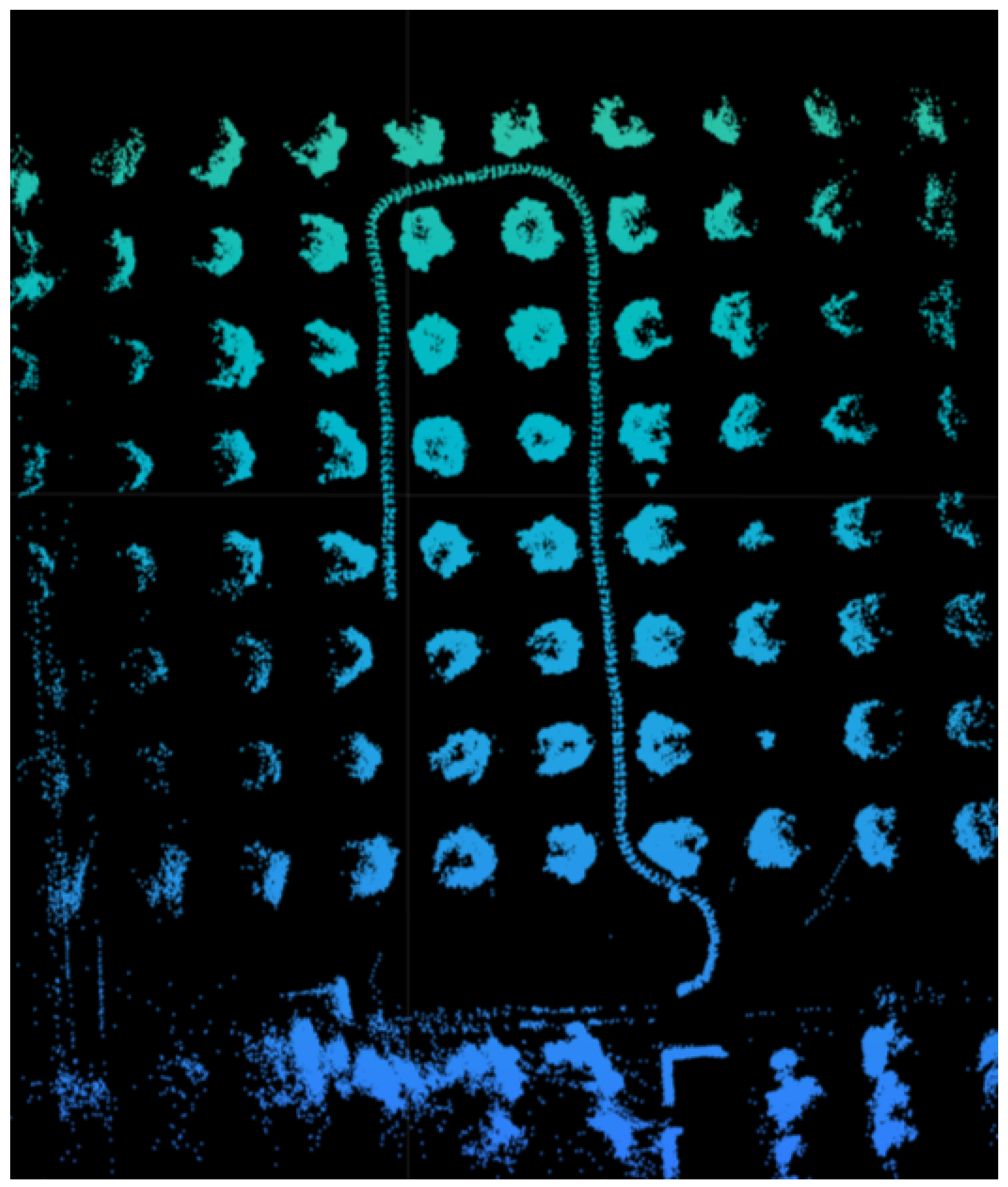
For this study, we selected a single sequence in which the robot navigates along a row of citrus trees. The complete point cloud and the corresponding robot path are shown in Figure 1. The dataset is publicly available at https://github.com/UCR-Robotics/Citrus-Farm-Dataset (accessed on 8 July 2025).

Implementation Overview

The implementation was carried out in MATLAB using the Robotics System Toolbox and the Computer Vision Toolbox. The processing pipeline comprises the following steps:

• Loading and Extracting Point Clouds: ROS bag files were loaded and point cloud messages were extracted to obtain raw LiDAR data.
• Point Cloud Merging: Individual scans were iteratively merged to form a unified point cloud of the environment, as shown in Figure 1.
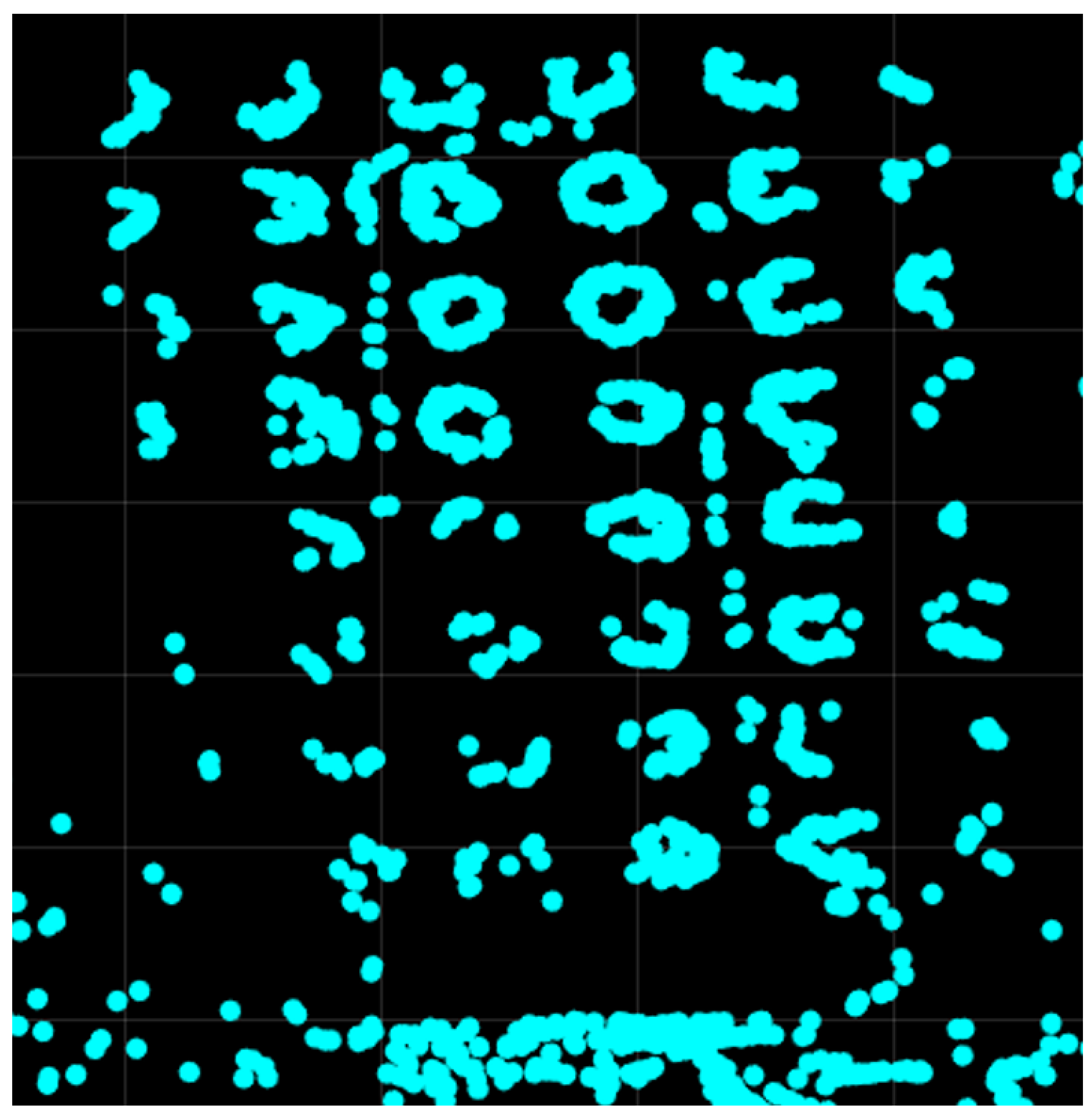
• 2D Projection and Graph Construction: The unified 3D point cloud was sliced horizontally into layers of fixed thickness, selected empirically to balance shape fidelity and computational cost. A representative slice is shown in Figure 2. Each slice was projected onto 2D and used to construct a graph where vertices represent points and edges encode inter-point distances. The Laplacian eigenvectors and eigenvalues were computed for each graph, enabling a frequency-domain representation of the point cloud.
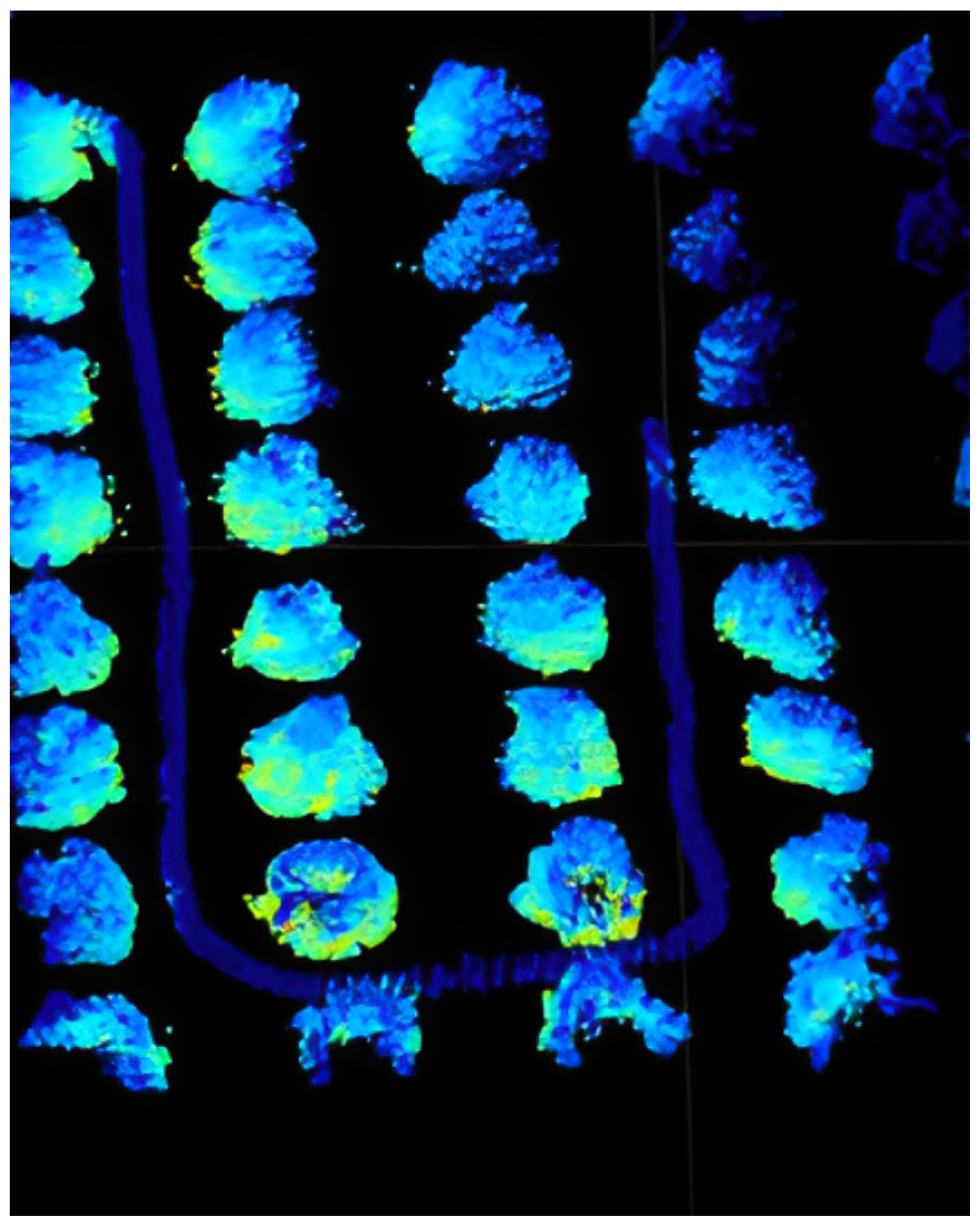
• Frequency Representation and Colour Mapping: Frequency components associated with each point in every slice were recorded. The point cloud was colour-coded based on these components, producing a frequency-based visualisation. As shown in Figure 3, lower frequencies (darker/blue) typically appear in linear and structured regions (e.g., the robot’s support frame), while higher frequencies (lighter/green) dominate chaotic areas such as canopies.
• Frequency Filtering: A band-pass filter was applied to isolate relevant frequency components. The objective was to determine whether certain frequency bands improve trajectory estimation performance. A systematic evaluation of all frequency band combinations was developed and is detailed in the next section.
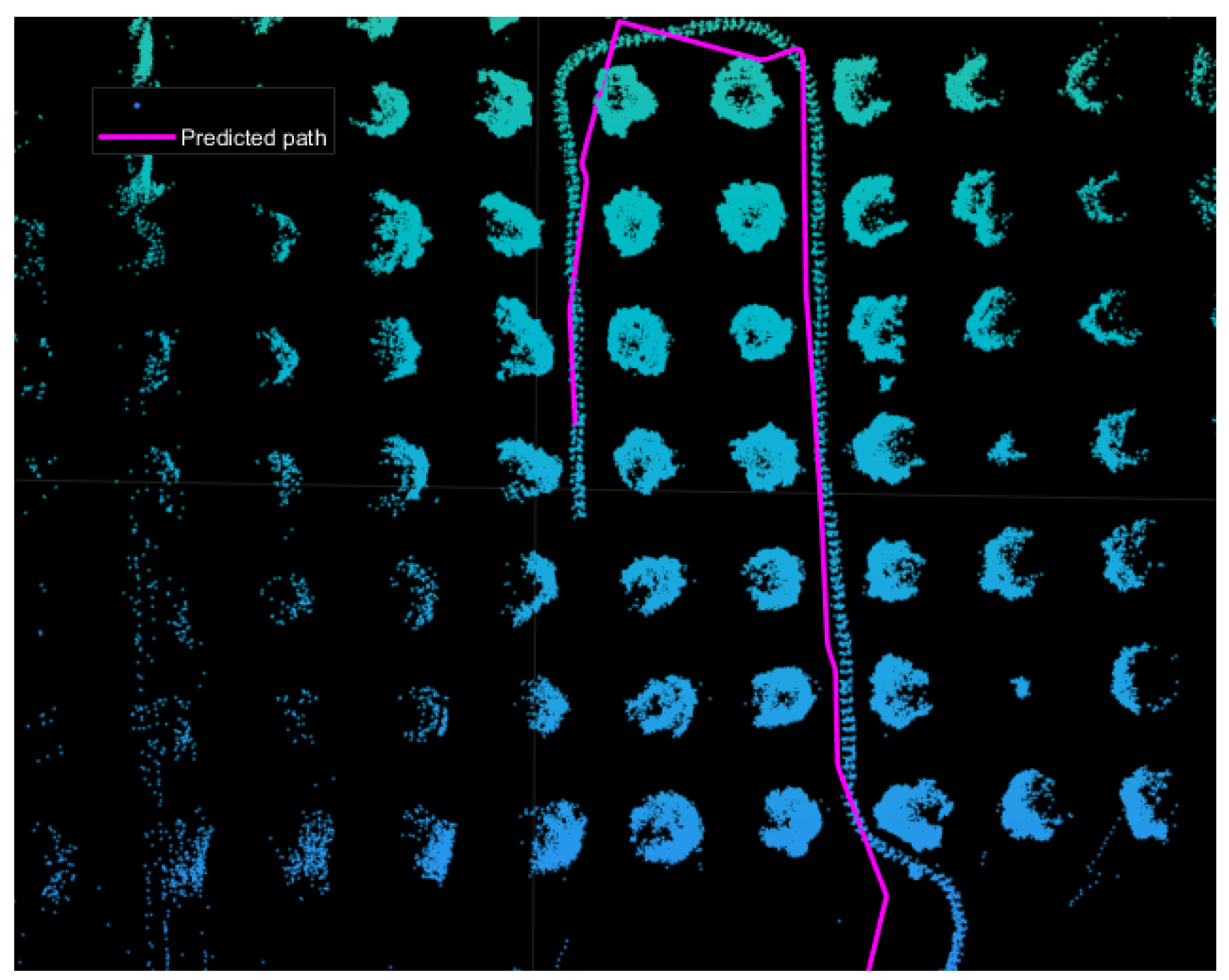
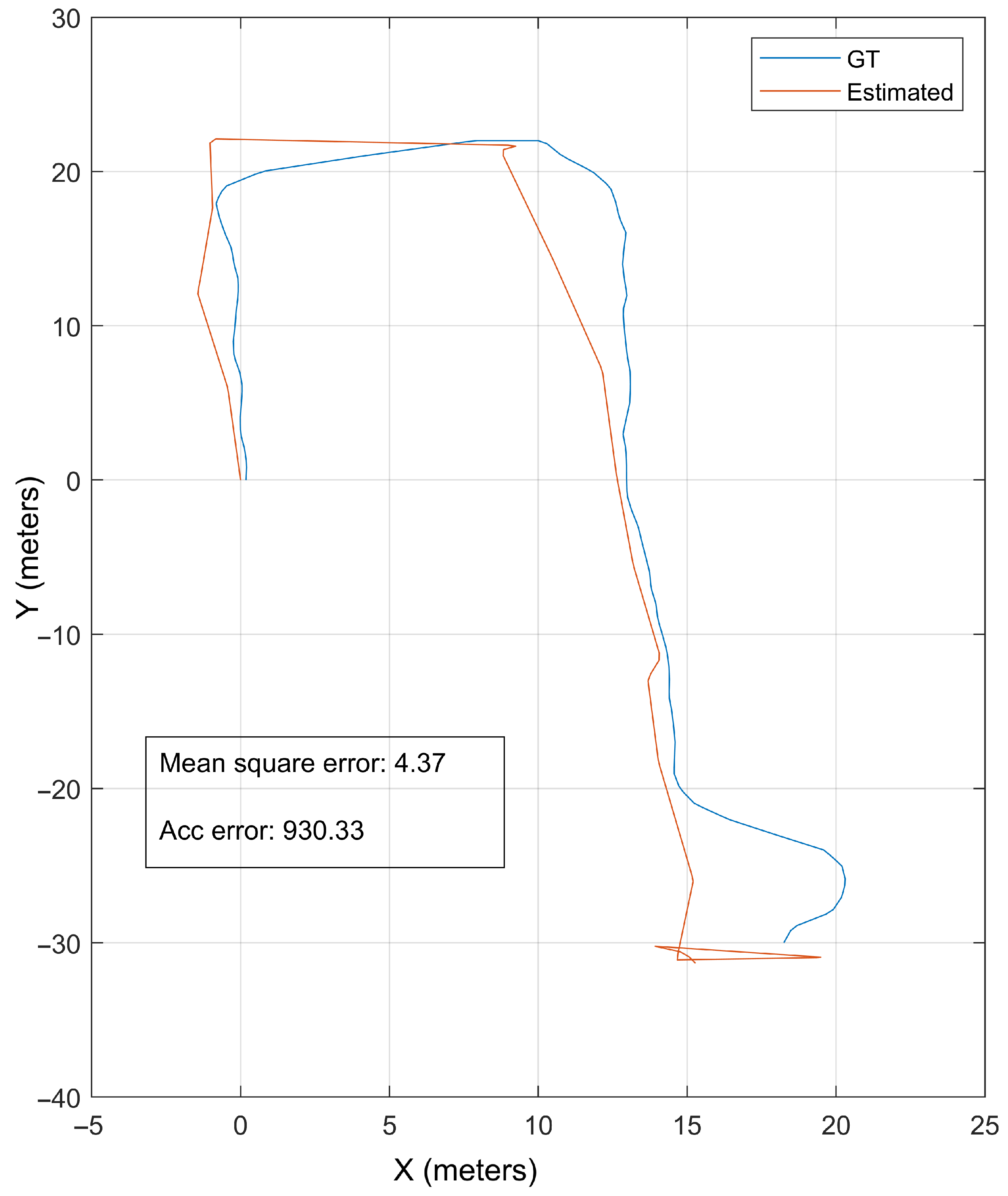
• Trajectory Estimation via ICP: The ICP algorithm was used to align consecutive scans and estimate the robot’s trajectory. By calculating the transformation (rotation and translation) between successive point clouds, a 3D path was reconstructed, as shown in Figure 4.

4.2. Dominant Frequency Determination

To identify the most informative frequency bands, we partitioned the frequency spectrum into segments and assessed their impact on ICP-based trajectory estimation. We began by dividing the frequency range into two bands and incrementally increased the number up to ten. This allowed for the examination of various filtering configurations, including low-pass, high-pass, and multiple band-pass options.

For each segmentation level, all combinations of frequency intervals were tested. A band-pass filter was defined based on each combination, and the resulting point cloud was fed into the ICP algorithm. The estimated trajectory was then compared to the ground truth and the mean squared error (MSE) recorded. All combinations were ranked based on their MSE performance.

4.3. Localisation Results

We first evaluated the baseline ICP trajectory estimation without any frequency filtering.

As shown in Figure 5, the ICP baseline produces a path with an MSE of 4.37 m. This value serves as a benchmark for evaluating frequency filtering strategies.

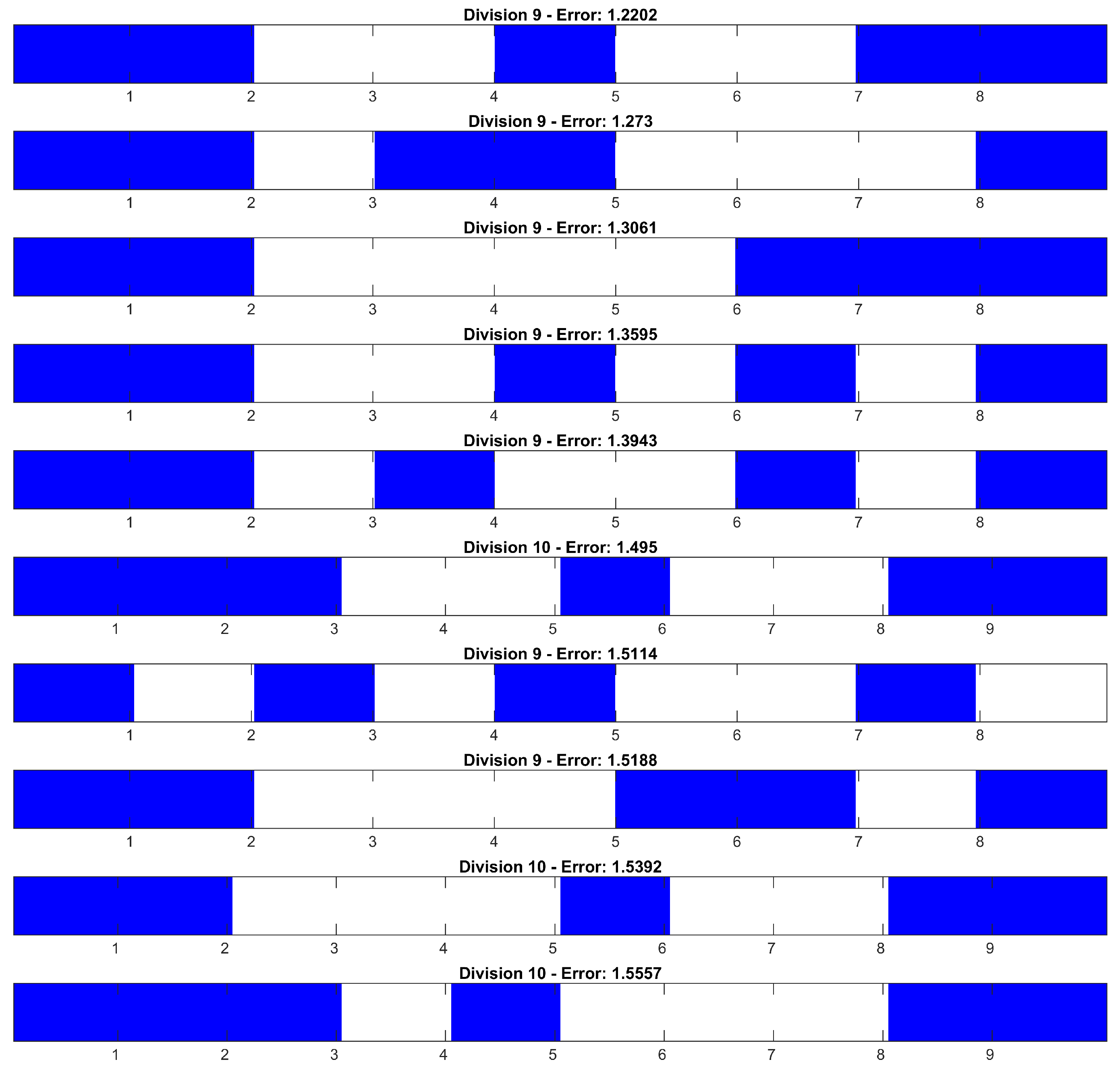
Figure 6 shows the ten best-performing frequency band combinations in terms of minimising MSE. Blue areas indicate the selected frequency intervals in each combination. Most high-performing combinations involve nine or ten bands, suggesting that finer spectral segmentation enhances performance. Notably, low and high frequencies appear consistently in top-performing combinations.

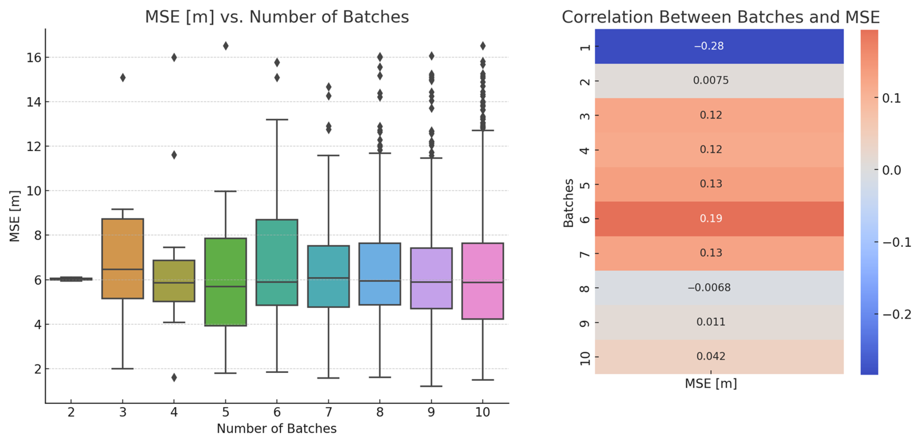
To better understand the impact of individual frequency bands on performance, we performed correlation analysis.

• Dummy Variable Encoding: Each frequency band was encoded as a binary variable indicating its presence in a combination.
• Correlation Calculation: Pearson correlation coefficients were computed between each band’s presence and the corresponding MSE, as shown in Figure 7.
• Visualisation: A heatmap was generated to illustrate correlations (Figure 8).

Key insights include:

• Batch 1: Strong negative correlation with error, indicating high utility.
• Batch 6: Strong positive correlation with error, suggesting reduced effectiveness.
• Batches 2 and 8: Near-zero correlation, indicating limited impact.
• Batches 3, 4, 5, 7, 9, 10: Moderate positive correlations, suggesting some detrimental effect.

To further analyse spectral importance, we subdivided the frequency range into 1000 narrow intervals and tallied how often each appeared in the 20 best combinations. The results, visualised as a heatmap (Figure 8), confirmed the importance of lower frequencies and the negative influence of the mid-spectrum (around Batch 6).

Despite the use of distinct analytical techniques, both correlation and frequency analyses agree: the lowest-frequency bands are the most informative for ICP-based localisation, while mid-range frequencies (especially around Batch 6) can mislead the registration.

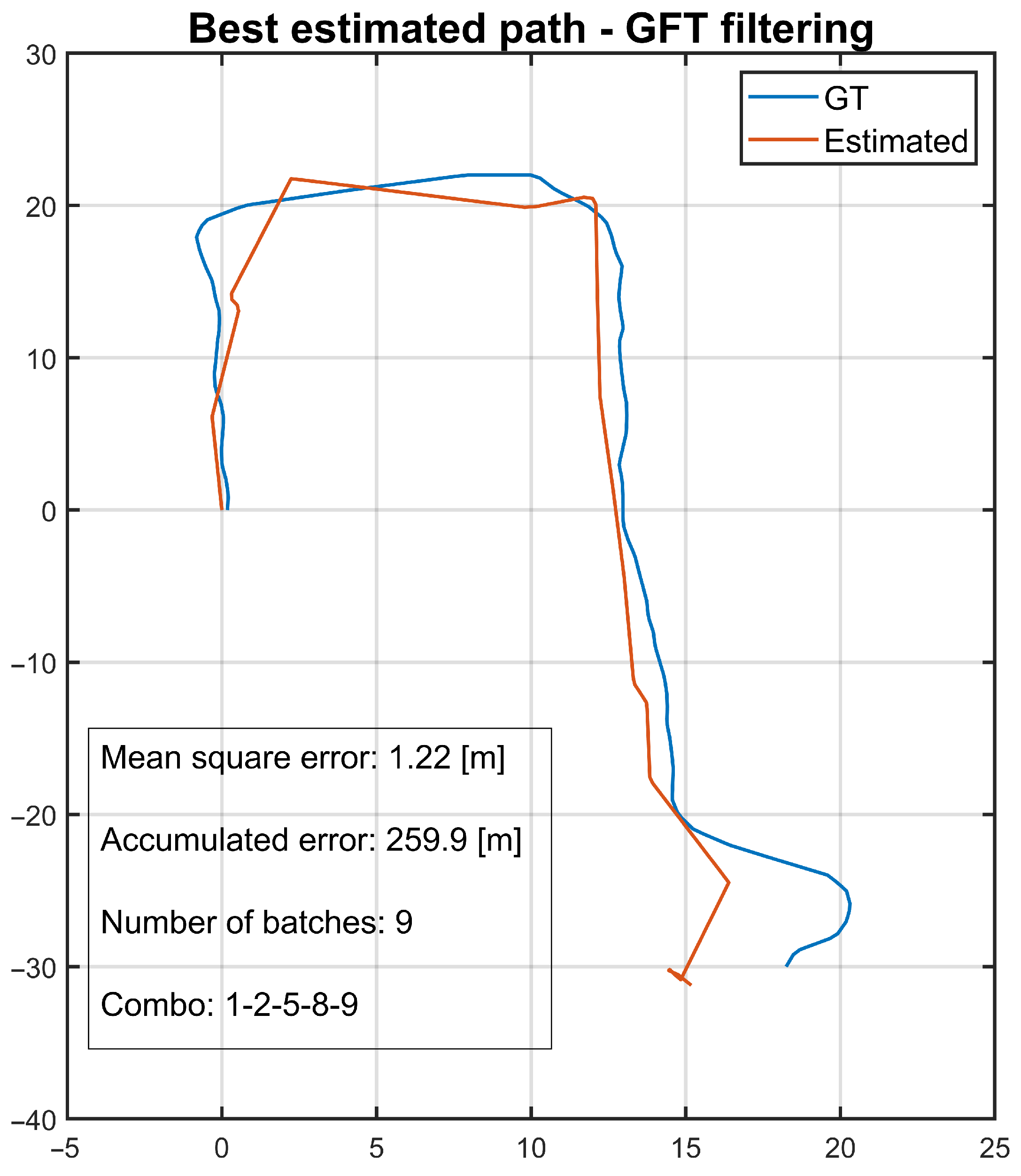
The final trajectory obtained using the best-performing frequency combination achieved an MSE of 1.22 m—an almost fourfold improvement over the unfiltered case. This result is shown in Figure 9.

5. Discussion

The results presented in this work highlight the potential of frequency-domain analysis for improving point cloud registration in unstructured, arboreal environments. By leveraging the Graph Fourier Transform (GFT) to decompose point clouds into frequency components, we were able to isolate and retain structural elements most relevant for localisation, such as tree trunks and ground surfaces, while suppressing less informative or noisy regions like canopies. This approach allowed the Iterative Closest Point (ICP) algorithm to achieve a localisation error of 1.22 m, a substantial improvement over the 4.37 m obtained with the unfiltered point cloud. In the following section, we present some of the advantages and limitations of our work.

5.1. Advantages

The frequency-domain filtering approach demonstrated significant improvements in localisation accuracy, reducing the error by approximately 72%, which validates the hypothesis that frequency decomposition enhances registration robustness in complex environments. This method offers a principled feature selection mechanism by isolating and preserving the most informative regions of the point cloud, thereby reducing computational burden through the exclusion of high-frequency noise and redundant data points. Additionally, the frequency-domain representation provides valuable interpretability by revealing the structural composition of the environment, effectively distinguishing between linear elements like tree trunks and more chaotic regions such as canopies. Beyond its application in agricultural settings, this framework is generalisable and can be adapted to various graph-based analyses, potentially extending its utility to urban or indoor environments where similar spatial characteristics exist.

5.2. Limitations

Despite its advantages, the proposed approach presents several limitations. The computation of the graph Laplacian and its eigendecomposition for each slice is computationally intensive, particularly when processing large-scale point clouds, even though the final ICP step benefits from reduced input data. Moreover, the method’s performance is sensitive to several parameters—including slice thickness, graph construction thresholds ($\tau$, $\sigma$), and the number of frequency bands—all of which require empirical tuning, potentially hindering reproducibility and robustness. The selection of optimal frequency bands remains a manual, heuristic process performed offline, limiting the method’s suitability for real-time or autonomous applications. Additionally, validation was conducted using a single sequence from the CitrusFarm Dataset, underscoring the need for further testing across diverse environments and sensor configurations to fully establish the generality and effectiveness of the approach.

6. Conclusions

This work explored a novel approach to point cloud registration by analysing point clouds in the frequency domain using graph signal processing techniques. It was demonstrated that selectively filtering specific frequency bands from the point cloud spectrum can significantly improve localisation accuracy in complex agricultural environments, as evidenced using the CitrusFarm dataset.

Experimental results show that applying band-pass filters based on frequency decomposition effectively reduces noise and enhances the extraction of relevant features for the Iterative Closest Point (ICP) algorithm, leading to a substantial reduction in localisation error compared to traditional processing without filtering. Furthermore, dominant frequency bands were identified that correspond to key structural elements of the environment, such as tree trunks and ground, which contribute positively to registration performance.

This frequency-domain approach opens new avenues for improving localisation and mapping techniques in GNSS-denied environments, where robustness and accuracy are critical. Future work includes integrating machine learning methods for adaptive frequency band selection and extending the methodology to other natural and urban scenarios.

References

- Li, Q.; Nevalainen, P.; Peña Queralta, J.; Heikkonen, J.; Westerlund, T. Localization in Unstructured Environments: Towards Autonomous Robots in Forests with Delaunay Triangulation. Remote Sens. 2020, 12, 1870. [Google Scholar] [CrossRef]
- Xia, S.; Chen, D.; Peethambaran, J.; Wang, P.; Xu, S. Point Cloud Inversion: A Novel Approach for the Localization of Trees in Forests from TLS Data. Remote Sens. 2021, 13, 338. [Google Scholar] [CrossRef]
- Tinchev, G.; Penate-Sanchez, A.; Fallon, M. Learning to see the wood for the trees: Deep laser localization in urban and natural environments on a CPU. IEEE Robot. Autom. Lett. 2019, 4, 1327–1334. [Google Scholar] [CrossRef]
- Tinchev, G.; Nobili, S.; Fallon, M. Seeing the Wood for the Trees: Reliable Localization in Urban and Natural Environments. In Proceedings of the 2018 IEEE/RSJ International Conference on Intelligent Robots and Systems (IROS), Madrid, Spain, 1–5 October 2018; pp. 8239–8246. [Google Scholar] [CrossRef]
- Fan, Z.; Zhang, L.; Wang, X.; Shen, Y.; Deng, F. LiDAR, IMU, and camera fusion for simultaneous localization and mapping: A systematic review. Artif. Intell. Rev. 2025, 58, 174. [Google Scholar] [CrossRef]
- He, X.; Pan, S.; Gao, W.; Lu, X. LiDAR-Inertial-GNSS Fusion Positioning System in Urban Environment: Local Accurate Registration and Global Drift-Free. Remote Sens. 2022, 14, 2104. [Google Scholar] [CrossRef]
- Zhuang, Y.; Sun, X.; Li, Y.; Huai, J.; Hua, L.; Yang, X.; Cao, X.; Zhang, P.; Cao, Y.; Qi, L.; et al. Multi-sensor integrated navigation/positioning systems using data fusion: From analytics-based to learning-based approaches. Inf. Fusion 2023, 95, 62–90. [Google Scholar] [CrossRef]
- Torres-Torriti, M.; Nazate-Burgos, P.; Paredes-Lizama, F.; Guevara, J.; Auat Cheein, F. Passive Landmark Geometry Optimization and Evaluation for Reliable Autonomous Navigation in Mining Tunnels Using 2D Lidars. Sensors 2022, 22, 3038. [Google Scholar] [CrossRef] [PubMed]
- Guevara, J.; Gené-Mola, J.; Gregorio, E.; Cheein, F.A.A. A systematic analysis of scan matching techniques for localization in dense orchards. Smart Agric. Technol. 2024, 9, 100607. [Google Scholar] [CrossRef]
- Ryu, J.; Kamata, S.-i. An efficient computational algorithm for Hausdorff distance based on points-ruling-out and systematic random sampling. Pattern Recognit. 2021, 114, 107857. [Google Scholar] [CrossRef]
- Guevara, J.; Auat Cheein, F.A.; Gené-Mola, J.; Rosell-Polo, J.R.; Gregorio, E. Analyzing and overcoming the effects of GNSS error on LiDAR based orchard parameters estimation. Comput. Electron. Agric. 2020, 170, 105255. [Google Scholar] [CrossRef]
- Li, Y.; An, J.; He, N.; Li, Y.; Han, Z.; Chen, Z.; Qu, Y. A Review of Simultaneous Localization and Mapping Algorithms Based on Lidar. World Electr. Veh. J. 2025, 16, 56. [Google Scholar] [CrossRef]
- Jiang, Y.; Wu, Y.; Zhao, B. Enhancing SLAM algorithm with Top-K optimization and semantic descriptors. Sci. Rep. 2025, 15, 8280. [Google Scholar] [CrossRef] [PubMed]
- Leanza, A.; Matranga, G.; Biddoccu, M.; Cavallo, E.; Milella, A.; Reina, G. Novel Measurements and Features for the Characterization of Soil Surface Roughness. IEEE Access 2022, 10, 131735–131746. [Google Scholar] [CrossRef]
- Liu, H.; Pan, S.; Wang, X.; Gao, W.; Yu, B.; Zhao, H. Long-Term Localization Method Integrated with Voxel Mapping LiDAR Odometry and Adaptive Updating Map in Diverse Environment. IEEE Trans. Instrum. Meas. 2025, 74, 8501914. [Google Scholar] [CrossRef]
- Lai, L.; Li, L.; Wang, H.; Yuan, J.; Fan, W.; Zhao, D. Enhanced LiDAR-inertial SLAM with adaptive intensity feature extraction and fusion. Meas. J. Int. Meas. Confed. 2025, 253, 117738. [Google Scholar] [CrossRef]
- Hong, Y.; Ma, R.; Li, C.; Shao, C.; Huang, J.; Zeng, Y.; Chen, Y. Three-dimensional localization and mapping of multiagricultural scenes via hierarchically-coupled LiDAR-inertial odometry. Comput. Electron. Agric. 2024, 227, 109487. [Google Scholar] [CrossRef]
- Li, Z.; Tong, P.; Shi, W.; Bi, X. Multi-Stage Registration and Feature Based Robust and Precise LiDAR SLAM; SAE Technical Papers; SAE International: Warrendale, PA, USA, 2025. [Google Scholar] [CrossRef]
- Xu, J.; Ma, Y.; Li, Y.; Zhang, X.; Zhou, J.; Yuan, S.; Xie, L. Dynamic Initialization for LiDAR-Inertial SLAM. IEEE/ASME Trans. Mechatron. 2025. [Google Scholar] [CrossRef]
- Zhu, D.; Wang, Q.; Wang, F.; Gong, X. Research on 3D LiDAR outdoor SLAM algorithm based on LiDAR/IMU tight coupling. Sci. Rep. 2025, 15, 11175. [Google Scholar] [CrossRef] [PubMed]
- CitrusFarm Dataset. Available online: https://registry.opendata.aws/citrus-farm (accessed on 8 July 2025).