Article

Intelligent Method for Generating Criminal Community Influence Risk Parameters Using Neural Networks and Regional Economic Analysis

1
Department of Scientific Activity Organization, Kharkiv National University of Internal Affairs, 27, L. Landau Avenue, 61080 Kharkiv, Ukraine
2
Department of Applied Mathematics, Ivan Franko National University of Lviv, 1, University Street, 79000 Lviv, Ukraine
3
Research Laboratory on the Problems of Legal Support of Police Activities and Combating Crime, Kharkiv National University of Internal Affairs, 27, L. Landau Avenue, 61080 Kharkiv, Ukraine
4
Department of Information Systems and Networks, Lviv Polytechnic National University, 12, Bandera Street, 79013 Lviv, Ukraine
5
Department of Education Quality Assurance, Kharkiv National University of Internal Affairs, 27, L. Landau Avenue, 61080 Kharkiv, Ukraine
6
Department of Postgraduate and Doctoral Studies, Zaporizhzhia National University, 66, University Street, 69063 Zaporizhzhia, Ukraine
*
Authors to whom correspondence should be addressed.
Algorithms 2025, 18(8), 523; https://doi.org/10.3390/a18080523
Submission received: 13 July 2025 / Revised: 31 July 2025 / Accepted: 14 August 2025 / Published: 18 August 2025
(This article belongs to the Section Analysis of Algorithms and Complexity Theory)

Abstract

This article develops an innovative and intelligent method for analysing the criminal community’s influence on risk-forming parameters based on an analysis of regional economic processes. The research motivation was the need to create an intelligent method for quantitative assessment and risk control arising from the interaction between regional economic processes and criminal activity. The method includes a three-level mathematical model in which the economic activity dynamics are described by a modified logistic equation, taking into account the criminal activity’s negative impact and feedback through the integral risk. The criminal activity itself is modelled by a similar logistic equation, taking into account the economic base. The risk parameter accumulates the direct impact and delayed effects through the memory core. To numerically solve the spatio-temporal optimal control problem, a neural network based on the convolutional architecture was developed: two successive convolutional layers (N1 with 3 × 3 filters and N2 with 3 × 3 filters) extract local features, after which two 1 × 1 convolutional layers (FC1 and FC2) form a three-channel output corresponding to the control actions UE, UC, and UI. The loss function combines the supervised component and the residual terms of the differential equations, which ensures the satisfaction of physical constraints. The computational experiment showed the high accuracy of the model: accuracy is 0.9907, precision is 0.9842, recall is 0.9983, and F1-score is 0.9912, with a minimum residual loss of 0.0093 and superiority over alternative architectures in key metrics (MSE is 0.0124, IoU is 0.74, and Dice is 0.83).

1. Introduction and Related Works

1.1. Relevance of the Research

In the modern world, the dynamic development of economic processes and parallel changes in the criminal situation largely determine a region’s socio-economic stability [1,2]. Research aimed at identifying the relationship between the economic activity level, the criminal community’s impact, and risk level is of particular importance in the global and local crisis context [3,4,5].
This research is relevant due to the need to find comprehensive and quantitative tools for analysis of socio-economic processes and management in unstable conditions. Mathematical modelling using optimal control methods [6] and neural networks [7,8,9] allows not only the identification of key patterns in regional development but also the development of recommendations for resource distribution to reduce risk. Such solutions are of particular importance for government agencies involved in ensuring security and economic growth since they allow them to respond quickly to emerging threats and minimise the negative consequences of crisis phenomena [10,11].
The integration of modern artificial intelligence methods with classical dynamics models opens up new prospects in solving spatial optimisation problems [12]. The neural networks used for these tasks provide numerical solutions that allow an increase in prediction accuracy and the optimisation of control actions’ costs [13,14,15]. In the constantly changing socio-economic context, such comprehensive and innovative approaches contribute to the formation of a sustainable mechanism for counteracting regional criminal activity and maintaining stable economic development.
Based on the above, this article proposes a mathematical model that integrates economic development parameters, crime intensity, and integral risk through differential equations with spatial diffusion and integral delays.

1.2. State of the Art

There are many research studies devoted to the analysis of relationships between economic development, criminal activity, and risk to social stability. Early research, for example [16,17], focused on these processes’ aspects, using classical logistic growth models to describe economic dynamics or statistical methods to analyse criminal activity. However, these researchers often did not take into account the complex interaction between various factors and did not provide sufficient integration within a single mathematical model.
Other research, such as [18,19,20], has attempted to combine economic and criminological dynamic elements through reaction–diffusion systems, which allowed spatial effects to be taken into account. Such approaches made it possible to model the spread of criminal phenomena across a territory and identify patterns in the risk geographic distribution. However, classical models often ignored lagging effects and nonlinear feedback, which play a significant role in the evolution of complex social systems.
In [21,22], economic growth is modelled using logistic equations, and crime dynamics are described using similar approaches. In this case, the criminal community’s influence on the economy was either taken into account as an external disturbance or was left outside the model framework. Such a simplified approach does not account for the possibility that a decrease in economic activity can stimulate the growth of criminal structures, and an increase in criminal activity, in turn, negatively affects the economic development dynamics [1,4,6,11].
Table 1 provides a comparison of the approaches considered.
Thus, the economic factors and criminal activity’s mutual influences on precise quantitative determination issues, as well as the relationship with the risk level, remain unsolved. Often, existing models, such as Refs. [16,19,21], do not include complex impact when a change in the system parameters has a multi-stage and delayed effect on other components. These studies lack an integrated approach that can take into account not only instantaneous changes but also their effect on dynamics, past states, and spatial diffusion influence accumulation.
The main problem is that traditional models [18,20] either consider the economy and crime as independent processes or try to combine them without taking into account nonlinear feedback. This leads to the fact that such models are not able to accurately predict the system’s evolution under external disturbances and internal fluctuations and do not provide adequate tools for optimal socio-economic stability management during crisis periods.
The developed method, based on modified logistic dynamics with additional terms taking into account criminal impacts, allows solving the problems mentioned above. The inclusion of extra terms in the equations makes it possible to model complex interactions, where a decrease in economic activity leads to an increase in the criminal structures’ influence, and an increase in criminal activity has a negative impact on financial parameters and increases the total risk. Thus, the method provides a more realistic display of the relationships in the socio-economic system dynamics.

1.3. Main Attributes of the Research

This research aims to develop an innovative intelligent method that can adequately describe the complex interaction between economic activity, criminal activity, and the risk-level dynamics of social stability.
The research object is regional-level socio-economic systems characterised by interconnected processes of economic development, criminal activity dynamics, and cumulative risk formation for society’s stability.
The research subject is an intelligent method based on modified logistic dynamics, which includes additional terms reflecting the criminal communities’ impact on economic activity and the total risk index.
The research’s main contribution is the integrated innovative intelligent method development that combines economic activity, criminal activity, and risk-level dynamics based on modified logistic dynamics with additional terms that take into account the criminal structures’ influence. The applied method allows us to effectively reflect nonlinear feedbacks, lagging effects, and spatial diffusion, which provides a more accurate prediction of socio-economic systems’ evolution and will enable us to assess the past states’ accumulated impacts. The integration of optimal control methods and neural network algorithms for the numerical solution of resource allocation optimisation problems opens up new prospects for rapid response in crises, contributing to both the modelling and practical risk management theoretical foundations’ improvement. The research’s scientific novelty lies in the integrated intelligent method development, which uses a modified logistic model for analysing the economic and criminal activity interaction using neural networks for the optimal control problem numerical solution, which allows us to take into account spatio-temporal factors and integral risks in real time.

2. Materials and Methods

2.1. The Economic Activity, the Criminal Communities’ Influence Intensity, and the Risk Parameter Method Development

Let the following main functions of time t characterise the area under consideration:
  • E(t) is the economic activity index or the economic development aggregate parameter (e.g., the investment, income, and employment level);
  • C(t) is the criminal community’s influence intensity (the criminal structures, their activity, and influence on economic activity);
  • I(t) is a risk parameter characterising the threat level to economic stability caused by criminal structures.
These functions are interconnected: a decrease in economic activity can stimulate the growth of criminal structures, and an increase in criminal influence can have a negative impact on the economy. The model aims to track the E(t) and C(t) dynamics and form the integral risk I(t).
To form the integral risk I(t) based on the E(t) and C(t) dynamics, it is necessary to develop the equilibrium state model with the control equilibrium states and spatial optimisation stability following determination.
The integral risk I(t) interaction dynamics model with the E(t) and C(t) dynamics is based on the following steps:
  • The basic logic of economic activity growth is determined by taking into account its naturally limited development, the negative impact of crime, and controlled external influence.
  • The reasons for the change in the criminal activity level are formulated, taking into account its dependence on the economic base, accumulated risk, and natural attenuation.
  • The integral risk accumulation mechanism is described by taking into account both current changes in the economy and crime, as well as the accumulated “memory” effect.
  • An equations vector system is formed, combining three variables and allowing us to analyse their joint dynamics and the influence of the control signals.
To determine the stability of equilibrium states, the following actions must be performed:
  • All possible stationary combinations of economic, crime, and risk levels are identified;
  • The model is linearised around each such state, minor deviations are introduced, and only linear terms are selected.
  • The Jacobian matrix is constructed to describe the system’s sensitivity to minor disturbances.
  • The characteristic equation is derived from the Jacobian matrix, which specifies the conditions under which disturbances decay or grow.
  • The stability criterion is applied, determining the parameters under which the system remains in equilibrium, and the Hopf bifurcation condition is formulated.
Control spatial optimisation is based on the following steps:
  • The research geographic area is designated, and the economic, criminal, and risk parameter dependence on coordinates and time is specified.
  • The spatial distribution of processes is taken into account through the diffusion operator, as well as distributed control actions.
  • A complete space–time equation system is written for all three variables, taking into account diffusion and control.
  • The initial and boundary conditions are determined for the correct formulation of the problem in a given territory.
  • The control quality target functional and the corresponding Hamiltonian with adjoint variables are formed.
  • The optimality conditions are derived, and the iterative algorithm “forward–backward” is described for finding optimal control strategies.
Based on [18,19], economic activity is represented by a modified logistic model, which includes a term describing the criminal community’s influence:
d E d t = α · E t · 1 E t K β · E t · C t + μ · I t · E t ,
where α > 0 is the economy’s introductory growth rate; K is the economic activity maximum (marginal) level (market capacity); β > 0 is the criminal communities negative impact amplification on the economy coefficient; and μ is the coefficient of risk parameter I(t) with a positive/negative external impact on the economy (if the risk is disturbing, then μ < 0).
The first term in (1) corresponds to logistic growth, the second to degradation due to criminal influence, and the third to additional adjustment according to the risk parameter (for example, the panic effect or, conversely, the investors’ mobilisation).
The C(t) dynamics are modelled by an equation similar to logistic dynamics [19], where the economic base influences the criminal group’s capabilities:
d C d t = ρ · C t · 1 C t γ · E t σ · I t + δ · C t ,
where ρ > 0 is the criminal communities’ “reproduction” rate (the activity’s probable expansion); γ > 0 is the coefficient linking the economic base with the potential for crime (the higher E(t), the greater the opportunities for recruitment, but also control by the state); σ is the risk of external impact (increase in criminal activity through external factors, such as corruption or external pressure); δ is the natural decrease in influence level (the law enforcement agencies, social programs, etc., conduct successful work).
The first term in (2) describes exponential growth with a limit proportional to economic activity, the second represents the increase in criminal activity due to general risk, and the third describes natural decay.
The risk index I(t) is characterised by an integral value [19] that accumulates the impact of changes in the economy and criminal activity, taking into account time delays. That is,
I t = I 0 + 0 t ω 1 · d E τ d τ ω 2 · d C τ d τ d τ ,
or in differential form:
d I d t = ω 1 · d E d t ω 2 · d C d t η · I 0 + 0 t g t τ · C τ d τ ,
where I0 is the risk parameter initial value; ω1 and ω2 > 0 are the coefficients of the change rate’s influence in economic activity and criminal activity on the risk; η > 0 is the risk attenuation coefficient (e.g., due to adaptation mechanisms or successful anti-criminal activity), and the integral term models the time lag. The function g(tτ) (memory kernel) describes how past values of criminal activity affect the current risk.
The “time duration” parameter is implemented through the memory kernel g(tτ), which weighs the economic and criminal activity’s past values’ contribution when calculating the integral risk I(t). The memory interval Tm length is specified a priori. It affects the kernel shape (e.g., exponential decay), which ensures earlier events impact weakening, and the time integrals themselves are reduced to an equivalent differential term in the risk equation. Thus, the accounting duration for past changes is controlled by the parameter Tm and the kernel decay coefficients, which allows the model to be adapted to analytical or empirical data on time delays in economic and criminal processes.
By combining Equations (1), (2) and (4), the following system is obtained:
d E d t = α · E t · 1 E t K β · E t · C t + μ · I t · E t , d C d t = ρ · C t · 1 C t γ · E t σ · I t + δ · C t , d I d t = ω 1 · d E d t ω 2 · d C d t η · I 0 + 0 t g t τ · C τ d τ ,
System (4) demonstrates complex interaction, where the following apply:
  • Changes in economic activity E(t) depend on its growth rates, criminal activity C(t), and feedback through the risk parameter I(t).
  • The criminal structures’ C(t) dynamics are defined as their exponential growth with a limitation depending on the economic base E(t), as well as external and internal factors.
  • The risk parameter I(t) accumulates information on the E(t) and C(t) current and past dynamics, reflecting both the direct impact of changes and the lagged effects.
When taking into account the spatial distribution, it is assumed that E(x, t) and C(x, t) are functions that depend not only on time, but also on the spatial coordinate x (location):
d E d t = D E · 2 E x 2 + α · E x , t · 1 E x , t K β · E x , t · C x , t + μ · I x , t · E x , t , d C d t = D C · 2 C x 2 + ρ · C x , t · 1 C x , t γ · E x , t σ · I x , t + δ · C x , t ,
where DE and DC are the corresponding quantities of the spatial diffusion coefficients.
To analyse the stationary stability solutions (E*, C*, I*), system (5) is linearised around the equilibrium points. For example, by setting
E ( t ) = E * + ϵ e ( t ) ,   C ( t ) = C * + ϵ c ( t ) ,   I ( t ) = I * + ϵ i ( t ) ,
a linear equation system for small perturbations was obtained:
d d t ϵ e t ϵ c t ϵ i t = J · ϵ e ϵ c ϵ i ,
where J is the Jacobian matrix, composed of the original system right-hand side’s first partial derivatives with respect to the variables E, C, and I.
The memory kernel g(tτ) can be chosen from a broad class of functions [19,22]. For example, this study proposes the use of the exponential kernel
g ( t τ ) = λ · e λ · ( t τ ) ,
then the integral term is represented as a convolution in the form:
0 t λ · e λ · t τ · C τ d τ ,
Expression (10) allows us to model the past criminal activity with exponential decay influence and an accumulation effect.
After developing an economic activity, criminal communities influence the risk parameter formation model. The next step is to analyse the system’s equilibrium states and stability and determine the stability boundaries. It will allow us to evaluate its response to minor disturbances and identify possible bifurcation points.

2.2. Determining the Stability Boundaries

To determine the stability boundaries, it is assumed that the system is defined by a trio of nonlinear equations based on (5):
d E d t = α · E · 1 E K β · E · C + μ · I · E , d C d t = ρ · C · 1 C γ · E σ · I + δ · C , d I d t = ω 1 · d E d t ω 2 · d C d t η · I .
The E*, C*, I* stationary (equilibrium) values are determined from the following conditions:
α · E * · 1 E * K β · E * · C * + μ · I * · E * = 0 , ρ · C * · 1 C * γ · E * σ · I * + δ · C * = 0 , ω 1 · d E d t E * , C * , I * ω 2 · d C d t E * , C * , I * η · I * = 0 .
The relations in system (12) define the equilibrium points around which the linearisation will be performed. For stability analysis, minor disturbances around the equilibrium point (7) are introduced and substituted into system (11). Under the ϵe, ϵc, ϵi smallness condition, the first-order terms remain, and the higher-order terms are discarded. As a result, a linear system for disturbance vectors is obtained, the form of which is entirely identical to (8). To determine the Jacobian matrix J elements, partial derivatives with respect to E, C, and I are calculated from the economic activity E(t), criminal activity C(t), and risk parameter I(t) equations (Table 2).
Thus, the Jacobian matrix J at the equilibrium point (E*, C*, I*) has the following form:
J = J 11 J 12 J 13 J 21 J 22 J 23 J 31 J 32 J 33 = α · 1 2 · E * K β · C * + μ · I * β · E * μ · E * ρ · C * 2 γ · E * 2 ρ 2 · ρ γ · C * E * δ σ ω 1 · J 11 ω 2 · J 21 ω 1 · J 12 ω 2 · J 22 ω 1 · J 13 ω 2 · J 23 η .
To determine the equilibrium state stability, the matrix J eigenvalues λ are calculated by solving the characteristic equation of the following form:
det(Jλ · I) = 0,
which has the form
λ3 + a1 · λ2 + a2 · λ + a3 = 0,
where the coefficients a1, a2, and a3 are expressed in the trace and minors of J terms, that is
a1 = −tr(J) = −(J11 + J22 + J33);
a2 = J11 · J22 + J11 · J33 + J22 · J33J12 · J21J13 · J31J23 · J32;
a3 = −det(J).
System (11) is considered asymptotically stable if all roots of the characteristic Equation (15) have negative real parts. A sufficient condition (provided that the coefficients are positive) is the Roy–Hurwitz inequalities:
a1 > 0, a3 > 0, a1 · a2 > a3.
Thus, the stability boundaries are determined by the points in the parametric space at which the equality is satisfied:
a1 · a2 = a3,
When one or more eigenvalues pass through the imaginary axis, by analysing the dependence of the coefficients a1, a2, and a3 on the model parameters (such as α, K, β, μ, ρ, γ, δ, σ, ω1, ω2, and η), it is possible to identify the boundaries at which the equilibrium state loses stability, for example, through bifurcations (passing through a critical point when the Roy–Hurwitz condition is violated). Passing through the stability boundary occurs when at least one of the Roy–Hurwitz conditions is violated. For example, when changing the parameter β (the crime influence intensity on the economy), a situation may arise when a1 · a2 = a3—this signals that the root λ becomes purely imaginary (λ = o · ω), which often precedes the oscillations’ development (the Hopf effect boundary state characteristic [23]).
By analysing the expressions for the Jacobian matrix elements and then the coefficients a1, a2, and a3, it is possible to construct the system’s stability dependence on the selected parameters. It allows us to both identify the parameters and critical values and to determine the conditions under which small changes in economic or criminal parameters can lead to a cascade of changes in the system.
After analysing the equilibrium state’s stability and determining the stability boundaries, the next step involves developing a spatial optimisation method that will take into account the process’s geographical distribution and optimise control based on the results obtained.

2.3. Development of a Spatial Optimisation Method

Let the territory under consideration be represented by a domain Ω ⊂ Rn (for example, n = 2 for the flat region map). The function E(x, t) characterises the economic activity at the local level, C(x, t) is the criminal communities’ local influence (activity), and I(x, t) is the local risk index, with x ∈ Ω, t ≥ 0. Then, the equations for economic activity (1), criminal activity (2), and the risk parameter (4) are presented as
d E x , t d t = D E · E x , t + α · E x , t · 1 E x , t K β · E x , t · C x , t + μ · I x , t · E x , t + U E x , t , d C x , t d t = D C · C x , t + ρ · C x , t · 1 C x , t γ · E x , t σ · I x , t + δ · C x , t + U C x , t , d I x , t d t = D I · I x , t + ω 1 · d E x , t d t ω 2 · d C x , t d t η · I x , t + Ω g x , y · C y , t d t + U I x , t ,
where DE > 0 is the diffusion coefficient for economic activity, Δ = ∇2 is the Laplace operator for spatial variables, UE(x, t) is the control action (e.g., financial support measures [20]), DC > 0 is the diffusion coefficient for criminal activity, UC(x, t) is the external control action (e.g., the law enforcement agencies operational measures [19,20]), DI > 0 is the diffusion coefficient for risk, Ω g x , t · C y , t d t is the integral term modelling the remote areas influence through the memory kernel g(x, y), e.g., the exponential kernel g(x, y) (e.g., the exponential kernel g x , y = λ · exp λ · x y [21]), and UI(x, t) is the control action in working terms with risk zones [19].
To solve the system, the initial distributions are given as
E(x, 0) = E0(x), C(x, 0) = C0(x), I(x, 0) = I0(x), x ∈ Ω,
and the boundary conditions on the boundary ∂Ω are given as Neumann conditions [24]:
d E d n Ω = 0 ,   d C d n Ω = 0 ,   d C d n Ω = 0 ,
where n is the derivative along the outward normal.
The spatial optimisation objective is to minimise the quality functional, which combines the parameters’ quadratic deviations from target values and the application of control actions. For this purpose, the target parameters are the target economy Etarget(x), minimisation of criminal activity C(x, t), and risk-level I(x, t) reduction. A functional of the following form is introduced:
J U E , U C , U I = 0 T Ω ω E · E x , t E t a r g e t x 2 + ω I · I x , t 2 + λ E · U E x , t 2 + λ C · U C x , t 2 + + λ I · U I x , t 2 d x d t ,
where ωE, ωC, and ωI > 0 are weighting coefficients for penalties for the parameter’s deviations, λE, λC, and λI > 0 are the cost coefficients for applying control actions, and T is the final optimisation time.
The optimisation aim is to minimise J under the condition that the system dynamics satisfy (19). Formally, the optimal control problem is defined as
min U E , U C , U I J U E , U C , U I
provided that the system (19) is satisfied with the given initial and boundary conditions. Here, the variables UE, UC, and UI are control functions that can be used to influence local dynamics. To identify priority zones from the total number of regional dynamics, the risk distribution I(x, t) is researched at the optimisation stage. For example, if we consider I(x, T) at a finite time T, we can calculate the critical region as
Ωcrit = {x ∈ Ω: I(x, T) ≥ Icrit},
where Icrit is the threshold risk value. Further, we can emphasise the additional control actions UC(x, t) and UI(x, t) in this zone.
To obtain optimal control actions U E * x , t , U C * x , t , and U I * x , t , a conjugate system of variables λE(x, t), λC(x, t), and λI(x, t) (Lagrange coefficients) is introduced, and a Hamiltonian of the following form is formulated:
H x , t = ω E · E x , t E t a r g e t x 2 + ω C · C x , t 2 + ω I · I x , t 2 + + λ E x , t · D E · E + α · E · 1 E K β · E · C + μ · I · E + U E + + λ C x , t · D C · C + ρ · C · 1 C γ · E σ · I + δ · C + + λ I x , t · D I · I + ω 1 · d E d t ω 2 · d C d t η · I + Ω g x , y · C y , t d t + U I + + λ E c · λ E 2 · U E 2 + λ C c · λ C 2 · U C 2 + λ I c · λ I 2 · U I 2 ,
where, in general, additional terms may be included to account for control costs. Necessary optimality conditions (Pontryagin maximum conditions) require that
H U E = 0 ,   H U C = 0 ,   H U I = 0 ,
and also, the conjugate equations are observed:
λ E t = δ H δ E ,   λ C t = δ H δ C ,   λ I t = δ H δ I .
To determine the optimal laws for UE(x, t), UC(x, t), and UI(x, t), the Hamiltonian (25) derivatives with respect to the control actions were calculated. When calculating the Hamiltonian (25) derivative with respect to UE, it was taken into account that UE is included in H(x, t) through two terms: in the linear term λE(x, t) · UE(x, t); in the quadratic term λ E c · λ E 2 · U E 2 . Taking the derivative, we obtained
H U E = λ E x , t + 2 · λ E c · λ E 2 · U E * x , t .
Condition (26) requires
λ E x , t + 2 · λ E c · λ E 2 · U E * x , t = 0 .
From (29), the optimal U E * x , t is determined:
U E * x , t = λ E x , t 2 · λ E c · λ E 2 .
The optimal law for UC(x, t) is defined similarly. Having calculated
H U C = λ C x , t + 2 · λ C c · λ C 2 · U C * x , t
assuming stationarity
λ C x , t + 2 · λ C c · λ C 2 · U C * x , t = 0 ,
the optimal form was obtained:
U C * x , t = λ C x , t 2 · λ C c · λ C 2 .
The optimal law for UI(x, t) is defined similarly. Having calculated
H U I = λ I x , t + 2 · λ I c · λ I 2 · U I * x , t
assuming stationarity
λ I x , t + 2 · λ I c · λ I 2 · U I * x , t = 0 ,
the optimal form was obtained:
U I * x , t = λ I x , t 2 · λ I c · λ I 2 .
For the solution’s completeness’s sake, we will also write down the conjugate equations’ general form that are obtained from the condition:
λ i t = δ H δ i ,   i = E , C , I .
That is, for λE(x, t) we have
λ E t = δ H δ E x , t .
In (38), the right-hand side includes partial derivatives of all terms of H with respect to E(x, t). For example,
δ H δ E = 2 · ω E · E x , t E t a r g e t x 2 + λ E x , t · α · 1 2 · E K β · C + μ · I + ,
as well as the contribution from the diffusion operator ΔE dependence and possible hidden dependencies in C · 1 C γ · E (when differentiating with respect to E).
For λC(x, t) and λI(x, t), the following is obtained in a similar manner:
λ C t = δ H δ C x , t , δ H δ C = 2 · ω C · C x , t + λ E x , t · β · E + λ C x , t · ρ · C · 1 C γ · E σ · I C + δ + + λ I x , t · Ω g x , y d y + ,
λ I t = δ H δ I x , t , δ H δ I = 2 · ω I · I x , t + λ E x , t · μ · E + λ C x , t · σ η · λ I x , t +
Thus, Equations (30), (33), (36), and (39)–(41), obtained from the condition H U i = 0 , represent the Pontryagin maximum condition’s central element for this optimal control problem. The values of the coefficients ωE, ωC, and ωI are responsible for the deviation’s relative importance from the desired trajectories or state values, and the terms with λ i c are introduced to account for the applied control costs.
Thus, the optimality conditions serve as the foundation for the justification and implementation of the iterative control algorithm. The optimality conditions set the necessary stationary relations between the control actions and the associated variables, ensuring the target functional gradients are calculated in each iteration “forward–backward”. Based on the optimality conditions, the control signals’ correction direction and magnitude are determined, which guarantees convergence to the optimal solution, taking into account the model’s physical and economic constraints.
Based on the above, a spatial optimisation method is proposed in the control problem context, whose structural diagram is presented in Figure 1.
The spatial optimisation method is a sequential system of blocks based on input data defining the domain geometry, variables E(x, t), C(x, t), and I(x, t), initial distributions, and model parameters, as well as target functions, for example, Etarget(x). On this basis, a mathematical model is formed that describes the variables’ dynamics, taking into account spatial diffusion, nonlinear effects, integral delays, and external influences. The quality functional, which combines current values squared deviations from target parameters and the application of control actions, serves as an optimisation criterion. Then, a Hamiltonian is formed, which summarises the cost functions, system dynamic equations, control actions, and the corresponding penalty terms; at the same time, the conjugate variables λE, λC, and λI are introduced for the Pontryagin maximum principle’s further application. Calculation of the optimality conditions (equating the Hamiltonian derivatives with respect to control actions to zero) allows us to obtain analytical expressions for the optimal control laws U E * x , t , U C * x , t , and U I * x , t . To correctly take into account the state’s influence on the system, adjoint equations are solved and integrated in the reverse direction, ensuring that all variational derivatives with respect to the model variables are taken into account. The iterative process based on the “forward–backward” scheme includes direct integration of the state dynamics equations with given initial conditions and backward integration of adjoint equations with control actions, subsequent updating, which leads to the quality functional minimising process’s convergence (Table 3).
As a result, this integrated approach ensures that the optimal control actions are received and that the system is controlled in the space–time domain, taking into account all input parameters and performance criteria.
Thus, the developed mathematical model describes the economic activity, criminal activity, and risk-level interaction dynamics. For the optimal control problem numerical solution, it is advisable to use a neural network model that approximates the necessary control actions. A neural network trained on the mathematical model basis effectively takes into account spatio-temporal dependencies. It allows for the optimisation of control in real conditions while maintaining physical limitations and observing the optimality criteria derived from the model.

2.4. Development of a Neural Network for the Optimal Control Problem’s Numerical Solution

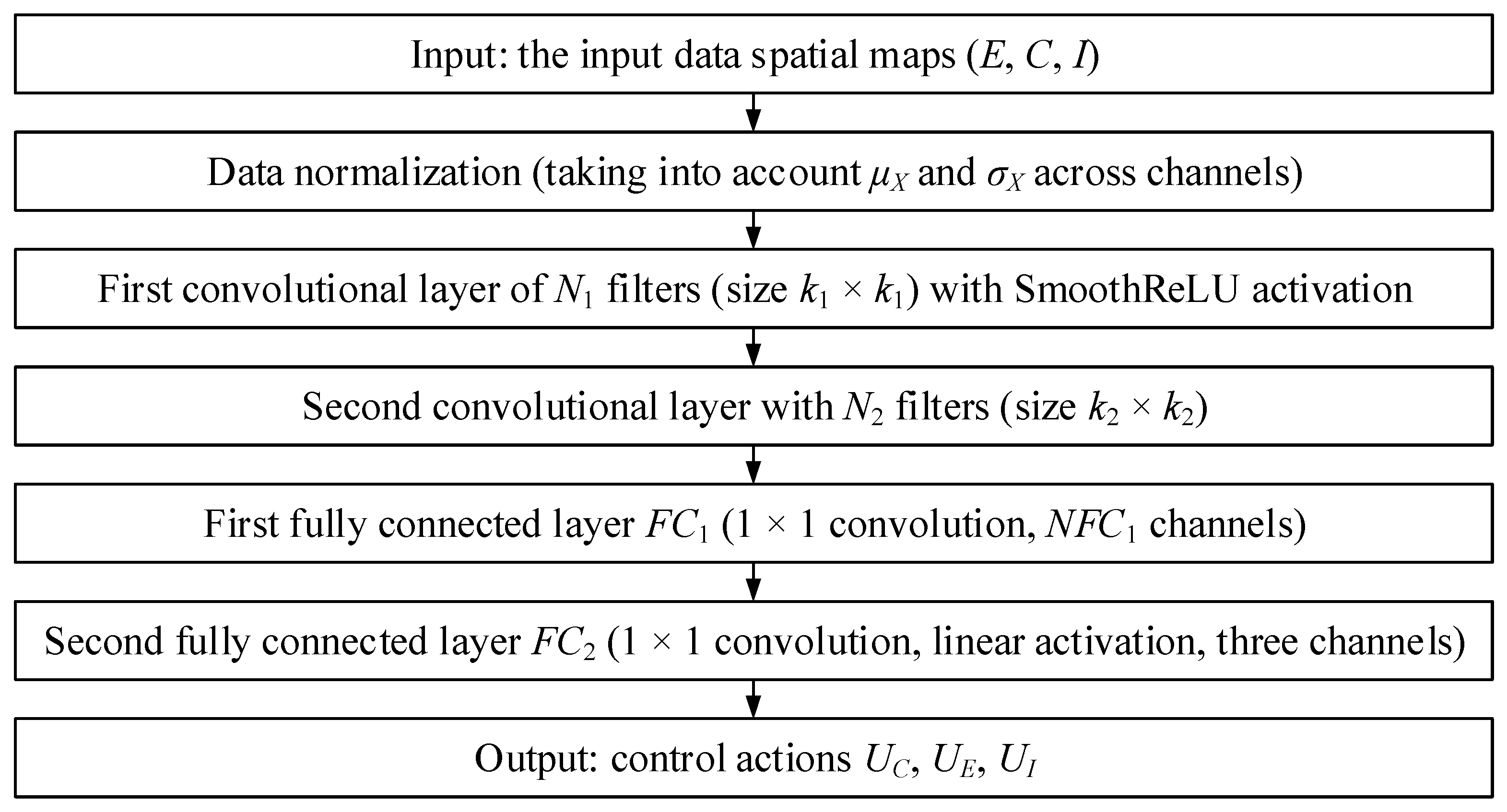
For the optimal control problem’s numerical solution aimed at identifying high-risk geographic areas and optimal resource allocation, a neural network model (Figure 2) was developed based on the architecture based on convolutional layers (Figure 3) for the spatial features’ extraction, to which fully connected layers were added to generate control signals UE, UC, and UI at each point. The developed neural network operates with spatial data (for example, in the two-dimensional maps or image form, where each pixel corresponds to the economic activity, criminal activity, and risk value). It produces optimal control actions for each point in the region.
The neural network model receives spatial maps characterising the economic activity, criminal activity, and risk-level parameters as input, which are pre-normalised by statistical parameters. The data then pass through the first convolutional layer, where local spatial features are extracted using N1 filters of size k1 × k1 and the SmoothReLU activation function [25,26]. This layer output goes to the second convolutional layer, equipped with N2 filters of size k2 × k2, which allows for the spatial features’ deeper extraction. The obtained features are then processed by a fully connected layer sequence implemented using 1 × 1 convolutions: the first layer (FC1) aggregates the features into a compact representation, and the final layer (FC2) with linear activation forms an output tensor containing three channels corresponding to control actions (UE, UC, UI).
Considering that a partial differential equations system determines the initial optimal control problem states E(x, t), C(x, t), I(x, t) and control actions UE(x, t), UC(x, t), UI(x, t) with the target quality functional:
J U E , U C , U I = 0 T Ω L E , C , I , U E , U C , U I d x d t ,
The problem is reduced to finding such control functions that minimise J under the partial differential equations’ dynamics condition.
The neural network is used to approximate the mapping:
E x , t , C x , t , I x , t U E x , t , U C x , t , U I x , t ,
In this case, the training process minimises some loss, taking into account both the error in fulfilling the optimisation conditions and the penalties for deviations from the specified target functions.
The function describes the developed neural network:
N: RH×W×m → RH×W×3,
where H and W are the spatial region dimensions (e.g., the pixels vertically and horizontally), m represents the input channels (e.g., m = 3 for maps E, C, and I), and the output channels are the control actions UE, UC, and UI.
The input tensor is a feature map:
X x = E x , t , C x , t , I x , t R H × W × 3 .
Provided that the input data is normalised, we can write
X ~ x = X x μ X σ X ,
where μX and σX are the mean and standard deviation vectors for each channel.
It is assumed that the first convolutional layer has N1 filters of size k1 × k1. For each i-th filter (where i = 1, …, N1), the output at position x = (x1, x2) is calculated as
Z i 1 x = σ j = 1 3 K i j 1 X ~ j x + b i 1 ,
where K i j 1 is the convolution (kernel) for the j-th input channel and the i-th filter, with dimensions k1 × k1; * is the convolution operation; b i 1 is the bias; σ is the SmoothReLU activation function [25,26]. The first layer output has dimensions H × W × N1.
For deep feature extraction, a second convolutional layer with N2 filters of size k2 × k2 is introduced similarly:
Z i 2 x = σ j = 1 3 K i j 2 * X ~ j x + b i 2 ,   i = 1 , , N 2 ,
after which an output tensor of size H × W × N2 is obtained.
Note: To improve the ability to extract spatial scales, standard practices such as “max pooling” [27] or “batch normalisation” [28] are used.
After the convolutional layers, two fully connected layers are applied (the FC1 layer is the 1 × 1 convolution; the FC2 layer is the 1 × 1 convolution with linear activation), implemented by convolution with a 1 × 1 kernel for each pixel, which allows preservation of the spatial structure.
In the FC1 layer (1 × 1 convolution), a 1 × 1 convolution is applied to combine features, that is
Z F C 1 x = σ W F C 1 · Z 2 x + b F C 1 ,
where W F C 1 R N F C 1 × N 2 and b F C 1 R N F C 1 . The output has size H × W × NFC1.
In the neural network output layer (layer FC2 is the 1 × 1 convolution with linear activation), it is necessary to obtain three channels corresponding to the control actions UE, UC, and UI. For this aim, a convolution with a 1 × 1 kernel without nonlinear activation is applied:
U E x , t U C x , t U I x , t = W F C 2 · Z F C 1 x + b F C 2 ,
where W F C 2 R 3 × N F C 1 and b F C 2 R 3 .
Thus, for each spatial position x ∈ Ω, the developed neural network model (see Figure 2 and Figure 3) produces a control action vector— U E x , t U C x , t U I x , t .
Since the original optimal control problem minimises the functional (42), when training the neural network, a loss function is specified, which consists of two components: the control actions approximation error and the penalty for violating the target functional.
Since there is a “target” control strategy U E * x , t , U C * x , t , and U I * x , t (for example, obtained by solving the adjoint system). Then the supervising loss is introduced in the following form:
L o p t = 1 Ω · x Ω U E x , t U E * x , t 2 + U C x , t U C * x , t 2 + U I x , t U I * x , t 2 .
In the target data’s absence, the loss function includes the partial differential equations system residual terms or the quality functional JPDE, which, based on [29,30], has the following form:
L P D E = Ω E t F E E , C , I , U E 2 + C t F C E , C , I , U C 2 + I t F I E , C , I , U I 2 d x ,
where FE, FC, and FI are the corresponding partial differential equations right-hand sides.
Then the neural network general loss function combines both terms (51) and (52) and is represented as
L = α · L o p t + 1 α · L P D E ,
where α is the weighting coefficient.
Based on the above, a neural network training algorithm was developed as presented in Table 4.
Thus, the developed neural network model (see Figure 2 and Figure 3) is a tool for an approximate solution to the optimal control problem, allowing the identification of high-risk geographic zones and the formulation of recommendations for the optimal distribution of law enforcement and social services resources. The optimality-oriented neural network model choice is justified by its ability to effectively solve the optimal control problem in the spatio-temporal distribution context, which is key to taking into account dynamic and interdependent factors such as economic activity, crime situation, and risk level. Unlike traditional optimised algorithms [14,20,23,24], which are usually based on fixed structures and assumptions, the neural network model provides flexibility in processing complex nonlinear dependencies and is able to adapt to changing conditions, which allows achieving more accurate solutions (accuracy reaches more than 90%) under high uncertainty and data variability conditions.

3. Case Study

3.1. Problem Statement

It is assumed that the system dynamics are defined by the following reaction–diffusion system (the model’s simplified version):
d E x , t d t = D E · E x , t + α · E x , t · 1 E x , t K β · E x , t · C x , t + μ · I x , t · E x , t + U E x , t , d C x , t d t = D C · C x , t + ρ · C x , t · 1 C x , t γ · E x , t σ · I x , t + δ · C x , t + U C x , t , d I x , t d t = D I · I x , t + ω 1 · α · E x , t · 1 E x , t K β · E x , t · C x , t + μ · I x , t · E x , t ω 2 · ρ · C x , t · 1 C x , t γ · E x , t σ · I x , t + δ · C x , t η · I x , t + U I x , t ,
where x = (x1, x2) ∈ Ω and t ∈ [0, T].
The model’s initial parameters are adopted in accordance with [19]: DE = 0.01, DC = 0.005, DI = 0.008, a = 2, K = 1, β = 0.5, μ = −0.3, ρ = 1.5, γ = 0.8, σ = 0.4, δ = 0.6, ω1 = 0.7, ω2 = 0.5, η = 0.2. The initial conditions (at time t = 0) are also adopted in accordance with the following [19]:
E x , 0 = 0.6 + 0.1 · sin 2 · π · x 1 · cos 2 · π · x 2 , C x , 0 = 0.2 + 0.05 · cos 2 · π · x 1 , I ( x ,   0 ) = 0.3 ,
where x = (x1, x2) ∈ [0, 1]2. In this case, for simplicity, the Neumann conditions (zero flow) in the form of (21) are assumed as boundary conditions.
The aim is, for example, to approximate the economic activity E(x, t) to within a given target distribution Etarget(x) (for example, a homogeneous value Etarget = 0.8) while minimising the C(x, t) and I(x, t) values and taking into account management costs. For this aim, the quality functional (22) is applied, in which wE = 1.0, wC = 0.5, wI = 0.5, and λE = λC = λI = 0.1 [19].

3.2. Selecting a Neural Network Architecture

As described in Section 2.4 “Development of a neural network for the optimal control problem’s numerical solution”, the developed neural network (see Figure 3) takes as input the tensor X x = E x , t 0 , C x , t 0 , I x , t 0 R H   ×   W   ×   3 and issue control actions U E x , t 0 , U C x , t 0 , U I x , t 0 R H   ×   W   ×   3 .
In the input layer, data normalisation is performed according to (46). The first convolutional layer contains N1 = 16 filters; the kernel size is k1 = 3 × 3. For each i-th filter (where i = 1, …, N1), Z i 1 x is calculated according to (47), giving the output at position x = (x1, x2). A similar calculation of Z i 2 x according to (48), is performed in the second convolutional layer containing N2 = 32 filters; the kernel size is k2 = 3 × 3. In the first fully connected layer FC1 (1 × 1 convolution), containing NFC1 = 64 channels, Z(FC1)(x) is calculated according to (49). In the output layer, which outputs three channels, UE(x, t), UC(x, t), and UI(x, t), the outputs are calculated according to (50).
Thus, the developed network approximates the optimal control strategy for the time t0, the initial moment.
To ensure fast convergence and stable training, we propose using the adaptive Adam optimiser with the following initial parameters: the learning rate is 1 · 10−3, the batch size is 32…64 samples (depending on the GPU memory size), and the epoch number is 100…150. This learning rate is high enough to effectively overcome the loss function plateau at early stages. Still, if necessary, it can be reduced to 1 · 10−4 using the learning rate decay scheme after 50…75 epochs for fine-tuning. A batch size of 32…64 will allow strengthening gradients over a sufficient number of examples while maintaining diversity within the batch, and 100…150 iterations over the entire dataset (epochs) will ensure convergence without significant overfitting, taking into account regularisation and validation curve control.
Algorithm 1 provides the algorithm’s pseudocode for the developed neural network training cycle.
Algorithm 1: The pseudocode of the NARX neural network training (author’s research).
Initialisation:
   set network architecture and initial weights W, b
   set combined loss function L = Lsup + α · Lres
Training cycle:
   for epoch = 1 to Epochs do
      for each batch X = {E(x), C(x), I(x)} from dataset do
         // Forward pass
         ŨE, ŨC, ŨI ← Network.forward(X)
         // Calculate losses
         Lsup ← ∥ŨE–UE_target∥^2 + ∥ŨC–UC_target∥^2 + ∥ŨI–UI_target∥^2;
         Lres ← PDE_residuals(E, C, I, ŨE, ŨC, ŨI);
         L ← Lsup + α · Lres;
         // Backpropagation
         gradients ← backprop(L)
         W, b ← optimizer.update(W, b, gradients)
   end for
   // (if needed) change learning rate
end for
Synthetic data were generated by numerically solving the reaction–diffusion equations system (54)–(55) with given parameters and Neumann boundary conditions, and the reference profiles UE, UC, and UI were calculated using the Pontryagin maximum principle using the optimal control iterative forward–backward scheme. Real data were obtained from the Ministry of Internal Affairs of Ukraine and economic development regional departments’ official reports for the period September–November 2024, aggregated to annual economic activity, crime rate, risk index parameters, and regions’ socio-demographic characteristics, followed by gaps’ imputation using the nearest neighbour method and the average for adjacent territories.
To ensure objective and reproducible calibration of the “base” levels (equilibrium states E*, C*, I*, weight coefficients ωE, ωC, ωI, and cost coefficients λE, λC, λI), the following unified procedure was used in the study: the diffusion parameters’ initial values (DE, DC, DI), model coefficients (α, K, β, μ, ρ, γ, σ, δ, ω1, ω2, η), and weight coefficients were taken from [19] (DE = 0.01, …, η = 0.2; wE = 1.0, wC = 0.5, wI = 0.5; λE = λC = λI = 0.1). For each of the three objective functions (economic control UE, crime prevention UC, and risk reduction UI), a structured enumeration of parameters (“grid search”) was carried out in the ±30% reference values range with a 10% step. For each option, the optimality criterion J was calculated, and the Roy–Hurwitz inequalities ensuring the basic state stability were checked. Based on the comparative analysis results, the loss weighted sum L (51) was minimised on the validation set, and, at the same time, the “forward–backward” algorithm convergence to the permissible threshold dL < 10−5 was controlled. The final parameters were chosen as a compromise between the J minimum value and reliable compliance with the stability conditions.

3.3. Data Collection and Preparation

The initial dataset for training the neural network was formed based on aggregated data obtained from various government sources. To create the dataset, statistical data from the Ministry of Internal Affairs of Ukraine and regional departments for economic development were used. The data was collected for the last 3 months (September, October, and November 2024) and includes parameters characterising economic activity, the criminal activity level, and the risk for the region. At the same time, each area is identified by a unique identifier, and the data time reference makes it possible to analyse the parameter dynamics over time. Since the sources could have different periodicities (quarterly/annual data), all parameters were aggregated at the yearly level. For quarterly ones, the sum (for example, the crime number) or the average (unemployment rate) was taken.
The initial dataset (Table 5) is presented in tabular form. It includes variables such as Economic_Activity, Criminal_Activity, and Risk_Index, as well as additional features reflecting the demographic situation (Population_Density), the law enforcement resources level (Police_Resources), and social factors (e.g., Youth_Unemployment). The data were obtained by combining official statistical reports, analytical reviews, and population surveys, after which the values were normalised and validated to ensure comparability of the parameters between regions. Missing values (e.g., regional statistics unavailability for a particular year) were replaced using the k-nearest neighbour imputation method (KNN imputation) [33,34,35], as well as averaging over neighbouring regions [36,37,38,39] with close Economic_Activity. The relations between “Criminal_Activity” and “Risk_Index” underwent logical control: Risk_Index ≥ f(Criminal_Activity), where f is the a priori basic dependence function [40], determined by experts from the Ministry of Internal Affairs of Ukraine.
Visualisation of key parameters for regions A01, A02, and A03 (Figure 4) shows a gradual decline in economic activity in all areas, with population density varying, reaching its highest values in A03 (Figure 4a). Figure 4b indicates increasing crime, particularly pronounced in region A02, where there is a police resource shortage. Figure 4c illustrates a sharp increase in the risk index in A02, which may signal the crisis onset.
Thus, the initial dataset contains the following features: Region_ID is a unique region identifier (integer encoding), for example, an administrative division code that allows the neural network to take into account the individual characteristics of each region. Time is a time index that takes values 0, 1, and 2, corresponding to the September (1), October (2), and November (3) months, which allows the neural network to take into account the dynamics over time as a numerical scale. Economic_Activity is the region’s economic activity measure, normalised based on such parameters as investment volume, production, and employment levels. Criminal_Activity is the criminal activity quantitative assessment, including data on the registered crimes’ number and their typology. Risk_Index is an aggregate risk index calculated taking into account the economic and criminal factors that influence it (for example, I = α · E + β · C). Population_Density is the population density, expressed as the inhabitant number per square kilometre, reflecting the demographic burden on the region. Police_Resources is the region’s provision relative value with law enforcement resources, for example, the police officers number per 1000 people, which indicates the law enforcement activity level. Youth_Unemployment is the youth unemployment rate, reflecting the region’s socio-economic problems. To prevent the neural network from “shifting” towards features with large absolute values (for example, population density), the min–max scaling [41,42] and Z-score normalisation [43,44] methods were used.
According to the min–max method, for each feature x from the training set, the following are calculated:
x m i n   = min i x i ,   x m a x   = max i x i ,
and a linear transformation was performed on the segment [0, 1]:
x = x x m i n   x m a x   x m i n   .
The min–max scaling method (56), (57) was applied to “Population_Density” and “Economic_Activity” (since they were unbounded from above and required maintaining proportions).
For features where relative variability around the mean is essential (e.g., “Criminal_Activity”, “Risk_Index”, “Youth_Unemployment”), the following standardisation was applied:
x = x μ σ ,
where µ and σ are the training dataset’s mean and standard deviation; it allows us to exploit information about how much the parameter deviates from the typical level.
Thus, if the distribution is close to uniform or has long tails, the min–max method is applied, and if the distribution is approximately standard, Z-score normalisation is applied.
All normalisation parameters (xmin, xmax, µ, σ) were saved and applied to the validation (amount is 20% of the training) and test (amount is 20% of the training) datasets without retraining. As a result, for each region in each year, there is a feature vector: [Region_ID, Time, Economic_Activity, Criminal_Activity, Risk_Index, Population_Density, Police_Resources, Youth_Unemployment] are the eight components in total. This format allows the neural network to simultaneously take into account spatial (Region_ID), temporal (Time), and quantitative (the remaining six normalised) characteristics.
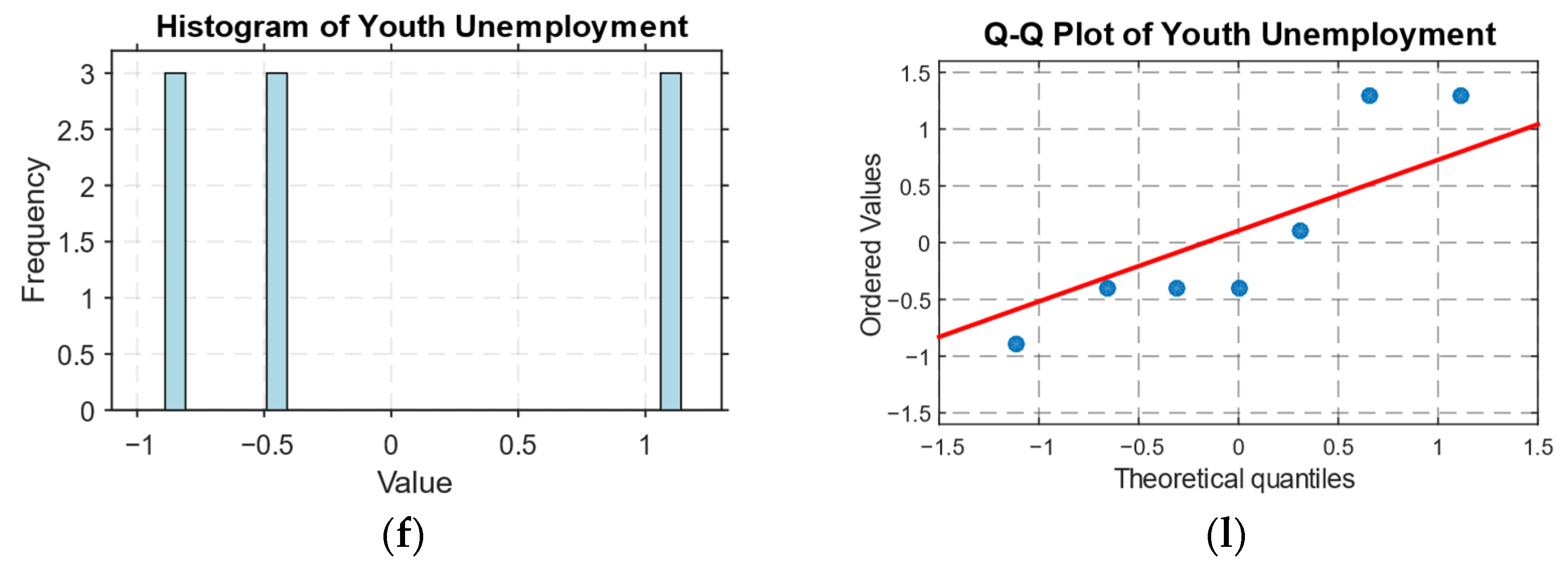
The preprocessing quality validation was carried out by visual inspection (histograms and QQ-plots of normalised features were constructed, Figure 5, where the “red dotted line” means the regression curve, and the “blue dots” are the experimental values obtained using the input dataset, presented in Table 5) and correlation analysis (Figure 6).
The histogram for the “Economic Activity” parameter shows a uniform distribution of values across the intervals—three observations are concentrated in the low range (0…0.1), one in each middle bin (0.5…0.6, 0.6…0.7, 0.7…0.8), and two in the upper bins (0.9–1.0), reflecting a relatively balanced change in economic activity in the dataset without sharp peaks or troughs; in the QQ-plot, the points lie close to the red line, deviating only slightly at the extreme quantiles, indicating a nearly normal distribution with light tails.
The histogram for the “Population Density” parameter shows three clear clusters at 0 (minimum), 0.5, and 1.0, a consequence of normalising the three repeating values of 950, 1200, and 1400 people/km2; the QQ density shows a slight shift at the extreme points, but overall, the clusters are within the expected range.
In the histogram for the “Police Resources” parameter, a similar three-modality (0, 0.667, 1.0) is reflected in the histogram, and the QQ points diverge only slightly in the upper part, which indicates the distribution homogeneity after normalisation.
The histogram for the standardised parameter “Criminal Activity” shows a right-hand tail: several points above +1.5, and a flat “bottom” on the left around −1.0; the QQ-plot highlights a slight positive asymmetry, as the upper quantiles extend slightly above the line.
The histogram for the “Risk Index” parameter also shows a moderately right-tailed distribution with density in the mid-range and rare values above +1.5; QQ points are located along the line in the centre, with minor deviations at the ends.
The histogram for the “Youth Unemployment” parameter has pronounced groups around −1.0, −0.7 and +1.3 in the histogram, and the QQ-plot shows a slight “hemisphericity” of the tails: above average, there are pointwise divergences, but without extreme outliers, all observations remain in the range from −1.3 to +1.3.
Thus, none of the visualisations revealed any outliers, and the QQ-plots generally confirm that the distributions are close to normal, with predictable deviations in the tails.
Correlation analysis showed that normalisation did not distort the fundamental relations between the key parameters: “Economic Activity” and “Criminal Activity” retain a strong inverse relation (r = −0.96), confirming that a decrease in crime accompanies an increase in economic activity; “Economic Activity” and “Risk Index” demonstrate an even stronger negative correlation (r = −0.97), which logically reflects a decrease in the overall risk in more developed regions; and “Criminal Activity” and “Risk Index” are in an almost perfect direct relation (r = +0.997), emphasising the crime rate contribution to the risk index formation. A comparison of the correlation matrices before and after normalisation shows the coefficients’ identical values, which proves the data structure’s correctness, scaling, and preservation.

3.4. Simulation Results

As part of the computational experiment, graphic elements were obtained that illustrate both the model’s main variables’ dynamics and the distribution of control actions in space and time. Figure 7 shows diagrams of the change in the average significance of E(t), C(t), and I(t) over time, on which basis both system dynamics analysis and stabilisation stage or crisis moment determination are carried out.
According to Figure 7, at the initial stage (t = 0), economic activity E(t) is at a level of about 1.6. In contrast, criminal activity C(t) is practically absent (close to 0), and the risk I(t) already reaches ~0.8. As C(t) grows in the interval 0 ≤ t ≤ 50 (where the red curve reaches a noticeable peak, about 0.5…0.6), the risk index I(t) (green line) also rises sharply and reaches a maximum at about t = 5. At the same time, E(t) (blue curve) decreases insignificantly and remains at a relatively high level (1.4…1.5), which, together with the increased criminal activity, maintains a high risk. After reaching a peak value in the time range t ≈ 5, crime C(t) declines, and along with it I(t) gradually decreases, as a result of which, by t = 10, the risk returns to moderate values (around 1.0…1.1). Economic activity E(t) ends the period in the 1.3…1.4 range.
Figure 8 shows the heat maps of the parameters E(x, t), C(x, t), and I(x, t), which visualise the economic activity level distribution across the territory (demonstrating fluctuations in economic activity in space and time) and the criminal activity intensity (showing an increased criminal activity localised zone), as well as regions with a high risk level (combining the economic and criminal factors’ influence, highlighting the greatest risk zones).
The economic activity E(x, t) distribution heat map (Figure 8a) shows significant regional differences: the diagram’s left part (at x ≈ 0) and the lower region (close to t ≈ 100) are dominated by low values, reflected in blue and green tones, indicating lower activity, while the upper central part (around x ≈ 20 and t ≈ 10) shows a distinct region with high values, characterised by rich yellow-green tones, indicating increased activity; on the right (around x ≈ 90) there is a mixed colour scheme, switching from purple to green tones, indicating a moderate decrease in E values in this region.
The criminal activity heat map, represented by the function C(x, t) (Figure 8b), demonstrates a characteristic “circular” distribution with a pronounced maximum (≈0.8) in the central area (approximately x ≈ 50, t ≈ 50), which indicates the criminal activity peak values in this central part in space and time; at the same time, the activity values gradually decrease to a minimum (approximately 0.1…0.2) on the periphery, covering both the extreme values along the spatial axis (x ≈ 0 and x ≈ 100) and the time’s early and late moments (t ≈ 0 and t ≈ 100), which allows us to conclude that the most dangerous zone is concentrated in the “middle” time interval and spatial location, while the territory edges and the period are characterised by a significantly criminal activity lower level.
The risk parameter map I(x, t), formed on the economic and criminal factors’ set basis (Figure 8c), demonstrates a characteristic distribution with a pronounced central “hot” area, similar to the criminal activity C(x, t) distribution. At the same time, the overall values slightly shift upwards (to approximately 2.25). In the central area, near the point (x ≈ 50, t ≈ 50), there is a maximum risk, indicated by a bright yellow colour. In contrast, on the periphery, at the edges along the x and t axes, the values decrease, which is visualised in a green-violet colour. Thus, the risk maximum (≈2.25) coincides with the most significant criminal activity areas and simultaneously indicates an increase in risk with an increase in economic activity, since I partially depends on E; moderate values (around 1.0…1.5) form a smooth transition to minimum values (around 0.5…0.75), which are observed in the lower left and upper right corners of the map, which emphasises the greatest risk concentration in the centre, where both studied parameters are intense.
The heat map summary interpretation (Figure 8) shows that the increased economic activity zone is located in the area x ≈ 20, t ≈ 15, where economic parameters are growing. Still, this area does not coincide with the risk “hot spot” found with extremely high criminal activity in the area x ≈ 50, t ≈ 50, which makes the most significant contribution to the overall risk index I. At the same time, the risk increases significantly in the central values, where there is a partial overlap with the economically active zone. Still, the correlation of risk with crime parameters remains much stronger, which is confirmed by the time structure: the risk and crime occur at a peak in intermediate time periods (t ≈ 50), while at the beginning and the end of the period under consideration (t ≈ 0 and t ≈ 100), crime and risk parameters decrease. In practice, this means that the optimal strategy in the law enforcement and social policy field is to concentrate efforts in the region’s central part and during the period when the risk reaches its maximum, while paying attention to supporting positive economic trends in the x ≈ 20, t ≈ 15 area to prevent crime’s negative impact.
Based on the heat maps, the diagrams of the control actions UE(t), UC(t), and UI(t) were obtained (Figure 9). The economic impact UE(t) represents measures aimed at stimulating or stabilising the economy through cyclical investments and government programs, which manifests itself in the smooth fluctuations form or changes in the intervention intensity over time; the anti-crime impact UC(t) is characterised by an impulse effect, with a pronounced peak moment (for example, during a special operation during the crime peak, t ≈ 5), reflecting the forces’ mobilisation with a subsequent decline after achieving the aim; the integral impact on risk UI(t) = α · UE(t) + β · UC(t) is these measures’ weighted combination, where α and β set the economic and criminal factors’ relative importance, providing a flexible risk containment strategy and reaching peaks at the active anti-crisis measures’ moments.
Figure 9 shows that the economic impact UE(t) (blue line) fluctuates around 0.5…0.55, reflecting a relatively stable economic support policy without sharp spikes. At the same time, crime suppression UC(t) (red line) has a pronounced peak around t = 5, indicating a targeted enhanced operation (special event). Overall, risk control UI(t) (green line) is built as a weighted combination of these strategies, so it also reaches a maximum around t = 5 and then smoothly returns to a low level. Thus, it can be said that economic measures are permanent. In contrast, anti-crime measures are concentrated in one period, due to which integrated risk control is concentrated exactly when it is most effective.
Figure 10 shows comparative diagrams of criminal activity and risk parameters before and after the intervention.
Figure 10 shows that before the intervention (dashed lines), crime C(t) (red dotted line) reaches about 0.5…0.6 peaks at t ≈ 5, and the risk index I(t) (green dotted line) rises above 1.6. After the introduction of the measures at point t = 5 (solid lines), criminal activity immediately falls by about 2…3 times, maintaining a lower level (below 0.3) until the period ends; following this, I(t) also significantly decreases, reaching only ~1.0…1.2 instead of 1.6. Thus, timely intervention effectively smooths out the crime wave peak and substantially reduces the subsequent risk.

3.5. The Neural Network Performance Evaluation

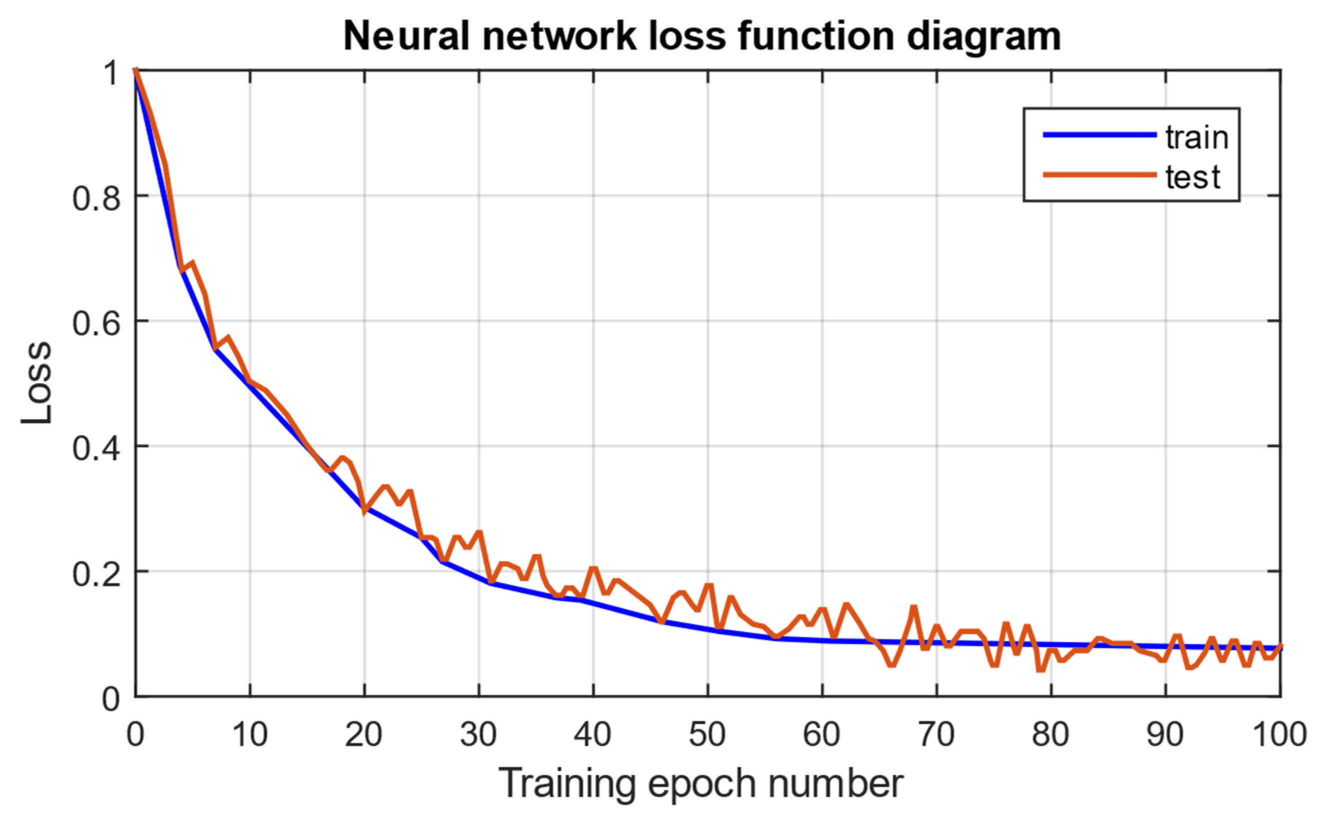
The loss function and the convergence of training estimate the neural network’s (see Figure 3) efficiency. Figure 11 shows the neural network loss function diagram, which shows the loss function L values on the training and validation datasets depending on the training epochs.
Figure 11 shows that at the training initial stages (epochs 1…10), the function value rapidly decreases from approximately 0.9 to 0.4, indicating a rapid improvement in the neural network parameters. Then, in the interval from 10 to 50 epochs, the decrease becomes more gradual as the losses stabilise in the range of 0.3…0.2. After the 50th epoch, the curve smoothing is observed with minor fluctuations around the value of ~0.15, indicating convergence and approaching a stable minimum. Thus, the model demonstrates good training ability and reaches a satisfactory optimisation level by the neural network’s middle training process.
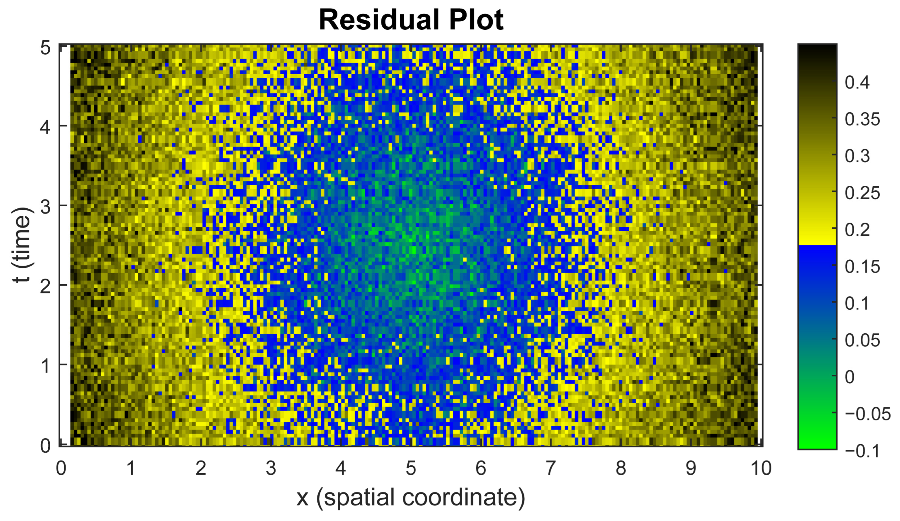
Figure 12 shows residual diagrams, revealing the difference between the left and right sides of the differential equations in the different parts of the domain.
Figure 12 shows the residual error distribution between the partial differential equation’s left and right parts, depending on the spatial coordinate x and time t. It is clearly seen that the most significant errors are concentrated at the domain edges: at the initial and final values of x and t, which is typical for boundary and initial conditions, where neural network models satisfy physical constraints less well. In the domain central zone (x ≈ 5, t ≈ 2.5), the residual errors are minimal, indicating good compliance with the physical model in these areas. This analysis allows us to localise zones that require additional training or the introduction of additional physical constraints.
The coefficient α = 1 was chosen as the weight between the control (“supervision”) and PDE-residual terms in (53) based on the preliminary experiment’s series in which the training quality was compared for different α = {0.1, 0.5, 1.0, 2.0}. For α < 1, the model converges faster in the supervision MSE (root mean square error ≈ 0.0124) terms, but the physical consistency deteriorates (residual loss increases above 0.015). For α > 1, the opposite effect is observed: residual loss decreases (<0.008), but MSE increases and convergence slows down (significant fluctuations in the loss function after 50 epochs). The optimal α = 1 provided balanced behaviour: residual loss ≈ 0.0093 and MSE ≈ 0.0124 with fast and stable convergence (loss stabilises around 0.15 by epoch 50).
Table 6 shows the developed neural network (see Figure 3) training results’ average values, as well as the accuracy parameter mean and variance values, where TP denotes the number of cases where the neural network correctly classifies a region as having a high risk (e.g., an area with a high crime rate where additional resources are needed), TN is the number of cases where the neural network correctly classifies a region as not having a high risk (e.g., an area with a low crime rate where resource allocation should be minimal), FP is the number of cases where the neural network incorrectly classifies a region as having a high risk, although in fact the risk is low (this may lead to resources unjustified redistribution to areas where they are not needed), and FN is the number of cases where the neural network incorrectly classifies a region as having a low risk, although in fact the risk level is high (this may lead to insufficient allocation of resources to the high-risk areas, which reduces the crime prevention measures or social problems effectiveness).
The results demonstrate that the model almost accurately identifies high-risk regions: accuracy = 0.9907, which means correct classification of 99.07% of cases, while precision 0.9842 ensures that 98.42% of all high-risk predictions actually correspond to real threats, and recall 0.9983 minimises the probability of missing such regions (false negative cases are almost absent), which is critical for timely and accurate resource allocation; while the high F1-score of 0.9912 emphasises the balance between accuracy and recall, and the average training time of 64 min and extremely low accuracy variance (0.00000103) indicate the model’s stability and reproducibility, which confirms its practical applicability in the operational response and crime prevention context.
Table 7 presents the various neural network architectures comparative analysis results based on accuracy key metrics, stability, and compliance with the modelled processes’ physical–semantic description. It allows us to evaluate the developed model’s effectiveness in the context of the influence of criminal communities on risk spatio-temporal analysis.
The data analysis presented in Table 7 demonstrates that the developed neural network outperforms alternative architectures in all key metrics covering temporal dynamics, spatial accuracy, compliance with physical-mathematical models, and robustness to network distortions. A significant decrease in the mean squared error (MSE = 0.0124) compared to LSTM (MSE = 0.0187), as well as a higher correlation of temporal patterns (0.91 vs. 0.79), indicates a risk dynamics more accurate reconstruction. Similarly, the spatial accuracy metrics (IoU = 0.74, Dice = 0.83) outperform the CNN, indicating improved recognition of high-risk geographic areas. At the same time, the residual minimisation in the differential equations (residual loss = 0.0093) and the high compliance with the conservation laws (0.96) demonstrate the model’s physical validity to a high degree. The classification metrics improved values in the diagram structure (node accuracy = 0.9735, F1-score = 0.9726) confirm the robustness to noise and the ability to take into account interregional relations. The results prove that the proposed architecture has high universality and applicability in the social and criminal nature of spatio-temporal risk complex analysis tasks.

4. Discussion

4.1. Obtained Results’ Evaluation

The three interconnected equation systems have been developed to describe the economic activity E(t), criminal influence C(t), and risk parameter I(t) dynamics. Economic activity is modelled by modified logistic growth taking into account degradation from criminal communities and feedback through risk (1), the criminal structures’ influence on dynamics is specified by a logistic equation in which growth is proportional to the economic base taking into account external and internal factors and natural attenuation (2), and the risk parameter accumulates the E and C change rates through the memory core g(tτ) in integral form and differential form taking into account the past states’ lagging effects (4). To research the system stability (5), it is written in the three nonlinear equations form (11), and the E*, C*, and I* stationary values are found from conditions (12). Then, linearisation is performed through the expansion E(t) = E* + εe(t), C(t) = C* + εc(t), I(t) = I* + εi(t) (7), which yields a linear system (8) with a Jacobian matrix J composed of the original Equations (13) and (16) right-hand sides’ first partial derivatives. The equilibrium stability is estimated by the eigenvalues λ, solving the characteristic equation det(Jλ · I) = 0 (14), or in the form λ3 + a1 · λ2 + a2 · λ + a3 = 0 (15), where a1 = −tr(J), and a2 and a3 are expressed through the J minors (16). According to the Roy–Hurwitz criteria, all roots have negative genuine parts when the inequalities a1 > 0, a3 > 0, a1 · a2 > a3 (17) are satisfied, and the stability boundaries are determined by the condition a1 · a2 = a3 (18).
In the research, it is assumed that the territory Ω ⊂ ℝ is considered through the space–time functions E(x, t), C(x, t), and I(x, t), described by the reaction–diffusion equations system with controlled effects UE(x, t), UC(x, t), and UI(x, t) (19), under the initial conditions E(x, 0) = E0(x), C(x, 0) = C0(x), and I(x, 0) = I0(x) (20), and Neumann boundary conditions (21). To assess the control quality, a functional J is introduced that combines the quadratic deviations from the target trajectories Etarget(x), the C and I minimisation, and the UE, UC, UI costs (22), and the optimal control problem itself is formulated as a J minimum with dynamics (19) (23) with the critical region allocation Ωcrit = {x ∈ Ω: I(x, T) ≥ Icrit} (24). Pontryagin’s maximum principle is implemented through the Hamiltonian H (25), which gives the optimality conditions H U E = 0 , H U C = 0 , and H U I = 0 (26) and the adjoint equations for λE, λC, and λI (27). Solving these conditions leads to the optimal control laws’ explicit expressions U E * (30), U C * (33), and U I * (36), which are implemented in an iterative “forward and backward” numerical solution algorithm.
A neural network model is proposed for the optimal control problem’s approximate solution, which approximates the mapping (44) with the input tensor (E, C, I) and outputs control actions (UE, UC, UI) (43) and (44); spatial features are extracted by two convolutional layers ((47) and (48); see Figure 2) followed by 1 × 1 convolutions FC1 and FC2 ((49) and (50); see Figure 3), and training is performed by means of a combined loss function, including the supervising component (51) and the partial differential equations residual terms (52), convolved into a common loss function L (53), which makes it possible to match the control functions’ approximation with the Pontryagin maximum principle and physical constraints of the optimal control system.
Based on aggregated statistical parameters of the Ministry of Internal Affairs of Ukraine and regional departments for September–November 2024, including “Economic_Activity”, “Criminal_Activity”, and “Risk_Index”, and additional demographic and social variables (“Population_Density”, “Police_Resources”, “Youth_Unemployment”), the initial dataset was formed, with the data being annualised (sum or average for quarterly parameters) followed by KNN imputation of missingness and normalisation: min–max scaling was applied to “Population_Density” and “Economic_Activity”, and Z-score standardisation was used to “Criminal_Activity”, “Risk_Index”, and “Youth_Unemployment”. The preprocessing correctness was confirmed by histograms and QQ-plot visual analysis for all features (see Figure 5), and the fundamental relations’ preservation was revealed through correlation analysis before and after normalisation (see Figure 6).
As the numerical experiment result, it was found that the E(t), C(t), and I(t) average values over time (see Figure 7) show that at t = 0 E ≈ 1.6, C ≈ 0, I ≈ 0.8, then C(t) reaches a peak of ≈ 0.5…0.6 at t ≈ 5, which is accompanied by a maximum increase in risk I(t), after which both functions gradually decrease, and E(t) remains at the 1.3…1.4 level. The spatial distribution heat maps (Figure 8) reveal that the maximum risk I ≈ 2.25 is localised in the central zone x ≈ 50, t ≈ 5. In contrast, the greatest economic activity zone is located at x ≈ 20, t ≈ 1.5. The control actions diagram (Figure 9) demonstrates the economy UE ≈ 0.5…0.55 with constant support, an anti-criminal measure UC pulse peak at t ≈ 5, and a combined profile UI with a maximum value at the exact moment. The dynamics before and after the intervention comparison (Figure 10) showed that after the measures, C(t) application decreased more than 2 times (below 0.3), and I(t) fell from ~1.6 to ~1.0…1.2, which confirms the proposed optimal control model’s effectiveness.
During the evaluation (see Figure 11), the loss function L on the training and validation datasets rapidly drops from ≈0.9 to ≈0.4 over the first 10 epochs, then stabilises at ≈0.2–0.3 and reaches ≈0.15 by the 50th epoch, indicating rapid convergence and the absence of overfitting; the residual errors distribution (see Figure 12) shows minimal residuals in the central region and their increase at the edges, which is typical for boundary conditions and confirms the model’s physical consistency. According to the testing results (Table 6), the neural network demonstrated accuracy = 0.9907, precision = 0.9842, recall = 0.9983, and F1-score = 0.9912. At the same time, the average training time was ≈64 min, and the accuracy variance was extremely low (0.00000103), which emphasises the proposed architecture’s high efficiency and stability.

4.2. Estimating Computational Complexity

The developed neural network architecture (see Figure 2 and Figure 3), applied to the optimal control problem numerical solution, includes two convolution layers and two 1 × 1 convolution layers. Let the input tensor take the size H × W × m, where H and W are spatial dimensions (e.g., 100 × 100), and m = 3 is the input channels (E, C, I). Then the total computational complexity estimate Ototal consists of the computational complexity sum of the neural network for each layer, O1O4.
The first convolutional layer with N1 = 16 filters and kernel k1 × k1 = 3 × 3:
O 1 = H · W · N 1 · m · k 1 2 = 100 · 100 · 16 · 3 · 9 = 4.32 · 10 6   o p e r a t i o n s .
The second convolutional layer with N2 = 32 filters and kernel k2 × k2 = 3 × 3:
O 2 = H · W · N 2 · N 1 · k 2 2 = 100 · 100 · 32 · 16 · 9 = 4.6 · 10 7   o p e r a t i o n s .
Fully connected layer FC1 with NFC1 = 64:
O 3 = H · W · N 2 · N F C 1 = 100 · 100 · 32 · 64 = 2.05 · 10 7   o p e r a t i o n s .
FC2 output layer with three channels:
O 4 = H · W · N F C 1 · 3 = 100 · 100 · 64 · 3 = 1.92 · 10 6   o p e r a t i o n s .
Thus, the total computational complexity for one forward pass is as follows:
O t o t a l = O 1 + O 2 + O 3 + O 4 7.6 · 10 7   o p e r a t i o n s .
Thus, the model has O H · W · N 1 · m · k 1 2 + N 2 · N 1 · k 2 2 + N 2 · N F C 1 + N F C 1 · 3 -order complexity, which, with standard input map sizes, fits into operations in the tens of millions and can be effectively implemented on modern GPUs or edge neural processors.

4.3. The Obtained Results in Practical Implementation

The results obtained in practical implementation and several key stages are highlighted in the article. The developed neural network allows for effective modelling and prediction of economic and criminal activity interaction, taking into account spatial and temporal factors (the accuracy exceeds 90%), which is vital for timely risk assessment and optimal resource allocation. As shown in Figure 7 and Figure 8, the changing dynamics in economic activity and crime rates can be used to identify high-risk areas where it is necessary to concentrate the law enforcement agencies’ and social services’ efforts. For example, the risk heat map (Figure 8) clearly demonstrates areas with the highest concentration of criminal activity, which allows for targeted anti-terrorism or law enforcement activities, as shown in Figure 9.
The computational experiment results based on training the neural network using real data from the Ministry of Internal Affairs of Ukraine demonstrate the model’s high accuracy (accuracy = 99.07%, precision = 98.42%, recall = 99.83%), which confirms its practical applicability for risk analysis and resource allocation at the regional level. The resulting diagrams and maps, such as Figure 10, show how criminal activity and risk can be reduced after interventions, which illustrates the proposed model’s effectiveness in real conditions.

4.4. The Obtained Results for Limitations and Prospects for Further Research

The results obtained have the following limitations:
  • The reaction–diffusion equation model (19) takes into account only the economic and criminal activity deterministic dynamics without random fluctuations or external noise, which limits its applicability in unpredictable crises and abrupt social change conditions.
  • The system’s linearisation around the stationary points (7) and (8) provides only local stability criteria and does not reflect possible behaviour under significant disturbances or bifurcations far from equilibrium.
  • The neural network preprocessing and training are based on data from only three months (September–November 2024), which reduces the prediction reliability for other seasons and long-term trends.
  • The residual errors distribution shows significant errors in the boundary conditions of the model (see Figure 12), which can lead to inaccuracies in areas with sharp gradients in economic or criminal parameters.
The limitations discussed above allowed us to formulate a roadmap for future research, presented in Table 8.
To confirm the method’s applicability, future research will also focus on introducing stochastic components, which will allow for random fluctuations and unpredictable social events using stochastic differential equations. Future research will also expand the time interval of the input dataset for training the model, which will reduce distortions caused by limited data and improve its generalisation ability under uncertainty.

5. Conclusions

An innovative intelligent method has been developed that combines the modified logistic dynamics of economic activity E(t), the criminal communities’ influence dynamics C(t), and the risk parameter I(t) through a reaction–diffusion equations system with lagging effects and spatial diffusion. An equilibrium state stability analysis has been carried out using linearisation and the Roy–Hurwitz criterion, determining the bifurcation boundaries when changing key parameters (β, σ, ω1, ω2, etc.).
In a numerical experiment with initial parameters (a = 2, K = 1, β = 0.5, μ = −0.3, ρ = 1.5, γ = 0.8, σ = 0.4, δ = 0.6, ω1 = 0.7, ω2 = 0.5, η = 0.2; DE = 0.01, DC = 0.005, DI = 0.008), it was shown that without intervention, C(t) reaches a 0.5…0.6 peak by t ≈ 5, and I(t) is 1.6…1.7, while E(t) smoothly decreases from 1.6 to 1.4. After applying optimal control actions, the C(t) level at the peak decreases to <0.3, and I(t) is ~1.0…1.2, which confirms the proposed “forward–backward” strategy’s effectiveness according to the Pontryagin maximum principle.
The E(x, t), C(x, t), and I(x, t) distribution heat maps revealed a “hot” risk zone in space—around x ≈ 50, t ≈ 5, where I reaches ~2.25—and a separate economically active area (x ≈ 20, t ≈ 1.5), which allows for anti-crime measures’ targeted concentration at the risk peak and supporting economic measures in the sustainable growth zone.
The developed neural network model (two 3 × 3 convolutions and 1 × 1 convolutions for UE, UC, and UI) demonstrated the optimal control strategies approximation with high accuracy: accuracy = 0.9907, precision = 0.9842, recall = 0.9983, F1-score = 0.9912, average training time of 64 min, and accuracy variance of ~1 × 10⁻⁶. When compared with LSTM (MSE = 0.0187 vs. 0.0124), classic CNN (IoU = 0.63 vs. 0.74; Dice = 0.71 vs. 0.83), PINN (residual loss = 0.0151 vs. 0.0093; conservation = 0.87 vs. 0.96), and GNN (node accuracy = 0.9735 vs. 0.9907; F1 = 0.9726 vs. 0.9912), the model showed the best performance in all key metrics.

Author Contributions

Conceptualisation, S.V., L.C. and T.R.; methodology, S.V., T.R., E.M. and A.B.; software, L.C., V.V., V.L. and A.B.; validation, E.M., T.R., V.V. and V.L.; formal analysis, L.C., E.M., T.R. and A.B.; investigation, S.V., V.V. and V.L.; resources, L.C., T.R., V.V., V.L. and A.B.; data curation, S.V., T.R., V.V. and V.L.; writing—original draft preparation, S.V. and T.R.; writing—review and editing, L.C., T.R., V.V. and A.B.; visualisation, L.C., V.V., V.L. and A.B.; supervision, L.C., E.M., T.R. and A.B.; project administration, S.V., L.C. and T.R.; funding acquisition, L.C. and V.L. All authors have read and agreed to the published version of the manuscript.

Funding

This research received no external funding.

Data Availability Statement

Data is contained within the article.

Acknowledgments

The research was carried out with the grant support of the Ministry of Education and Science of Ukraine “Methods and tools for detecting disinformation in social networks based on deep learning technologies” under Project No. 0125U001852.

Conflicts of Interest

The authors declare no conflicts of interest.

References

  1. Cretu-Adatte, C.; Azi, J.W.; Beaudet-Labrecque, O.; Bunning, H.; Brunoni, L.; Zbinden, R. Unravelling the Organisation of Ivorian Cyberfraudsters: Criminal Networks or Organised Crime? J. Econ. Criminol. 2024, 3, 100056. [Google Scholar] [CrossRef]
  2. Béchervaise, N.E.; Benjamin, C.G. Visionary or Criminal: From Profit through Morality to Socially Sustainable Entrepreneurship. Procedia-Soc. Behav. Sci. 2013, 99, 339–350. [Google Scholar] [CrossRef]
  3. Street, B. The Impact of Economic Opportunity on Criminal Behavior: Evidence from the Fracking Boom. J. Public Econ. 2025, 248, 105402. [Google Scholar] [CrossRef]
  4. Croci, G.; Gomez, J. Breaking the Cycle: The Role of the Criminal Justice System in Understanding Homicide Rates. J. Crim. Justice 2025, 99, 102450. [Google Scholar] [CrossRef]
  5. Han, H.; Zhang, P.; Liu, C.; Zheng, Y. Financial Technology Development, Regional Marketization, and the Effectiveness of Criminal Investigation Cases. Financ. Res. Lett. 2025, 81, 107459. [Google Scholar] [CrossRef]
  6. Ibrahim, O.M.; Okuonghae, D.; Ikhile, M.N.O. A Mathematical Model of Criminal Gang Rivalry: Understanding the Dynamics and Implications. Results Control Optim. 2024, 14, 100398. [Google Scholar] [CrossRef]
  7. Yin, L.; Liu, R. A Normalized Deep Neural Network with Self-Attention Mechanisms Based Multi-Objective Multi-Verse Optimization Algorithm for Economic Dispatch. Appl. Energy 2025, 383, 125414. [Google Scholar] [CrossRef]
  8. Vladov, S. Cognitive Method for Synthesising a Fuzzy Controller Mathematical Model Using a Genetic Algorithm for Tuning. Big Data Cogn. Comput. 2025, 9, 17. [Google Scholar] [CrossRef]
  9. Vladov, S.; Vysotska, V.; Sokurenko, V.; Muzychuk, O.; Nazarkevych, M.; Lytvyn, V. Neural Network System for Predicting Anomalous Data in Applied Sensor Systems. Appl. Syst. Innov. 2024, 7, 88. [Google Scholar] [CrossRef]
  10. La Rocca, M.; Fasano, F.; Staglianò, R.; La Rocca, E.T.; Deloof, M. The Financial Life Cycle of European SMEs before, during and after Crisis Periods. What Is the Role of a Country’s Financial System? Int. Rev. Financ. Anal. 2025, 104, 104342. [Google Scholar] [CrossRef]
  11. Prievozník, P.; Strelcová, S. The Impact of Crisis Phenomena on Economic Security in the Automotive Industry and the Quality of Life of Employees. Transp. Res. Procedia 2023, 74, 1412–1418. [Google Scholar] [CrossRef]
  12. Luan, C.; Liu, R. Integrated Ecological and Environmental Spatial Soft Constraint Mechanism: Urban Multi-Objective Land Use Optimization under Multiple Scenarios. J. Environ. Manag. 2025, 385, 125661. [Google Scholar] [CrossRef]
  13. Oh, S.; Choi, A. How Does Divergence of Control and Cash-Flow Rights Influence Cost Stickiness? Br. Account. Rev. 2025, 57, 101495. [Google Scholar] [CrossRef]
  14. Moloudpourfard, B.; Zarandi, M.T.; Pouyakian, M. Updating the “Cost Factor” in the William Fine Risk Assessment Method Following Economic Power: A Case Study of Selected Production Industries in Iran. Heliyon 2025, 11, e42405. [Google Scholar] [CrossRef]
  15. Calabrò, F.; Minniti, G.E.; Fotia, A.; Pucinotti, R. Recovery of Historic Real Estate: Life Cycle Costing and Economic Feasibility. Procedia Struct. Integr. 2024, 64, 1759–1766. [Google Scholar] [CrossRef]
  16. Drydakis, N. Business Disruptions Due to Social Vulnerability and Criminal Activities in Urban Areas. J. Crim. Justice 2024, 95, 102293. [Google Scholar] [CrossRef]
  17. Huang, H.; Xu, X.; Du, S. Can Financial Innovation and Industrial Structure Upgrading Reduce Regional Criminal Activity Levels? Financ. Res. Lett. 2025, 75, 106862. [Google Scholar] [CrossRef]
  18. Tonkonoff, S. Crime as Social Excess. Hist. Hum. Sci. 2014, 27, 60–74. [Google Scholar] [CrossRef]
  19. Stephan, A. The Cartel Trial: Issues of Dishonesty and Jury Nullification. J. Compet. Law Econ. 2023, 19, 312–332. [Google Scholar] [CrossRef]
  20. Telep, C.W.; Weisburd, D.; Gill, C.E.; Vitter, Z.; Teichman, D. Displacement of Crime and Diffusion of Crime Control Benefits in Large-Scale Geographic Areas: A Systematic Review. J. Exp. Criminol. 2014, 10, 515–548. [Google Scholar] [CrossRef]
  21. Zakaria, A.; Osman, S.; Etwire, C.J.; Makinde, O.D. Modeling the Dynamics of Some Common Reported Offenses by the Ghana Police Service. Partial Differ. Equ. Appl. Math. 2025, 14, 101171. [Google Scholar] [CrossRef]
  22. Mamo, D.K.; Kinyanjui, M.N.; Teklu, S.W.; Hailu, G.K. Mathematical Modeling and Analysis of the Co-Dynamics of Crime and Drug Abuse. Sci. Rep. 2024, 14, 26461. [Google Scholar] [CrossRef]
  23. Rehman, A.; Wu, R. Hopf–Hopf Bifurcation of the Memory-Based Diffusive Bacterial Infection Model. Phys. D Nonlinear Phenom. 2025, 476, 134653. [Google Scholar] [CrossRef]
  24. Provatidis, C.; Eisenträger, S. Macroelement Analysis in T-Patches Using Lagrange Polynomials. Mathematics 2025, 13, 1498. [Google Scholar] [CrossRef]
  25. Vladov, S.; Scislo, L.; Sokurenko, V.; Muzychuk, O.; Vysotska, V.; Osadchy, S.; Sachenko, A. Neural Network Signal Integration from Thermogas-Dynamic Parameter Sensors for Helicopters Turboshaft Engines at Flight Operation Conditions. Sensors 2024, 24, 4246. [Google Scholar] [CrossRef]
  26. Vladov, S.; Sachenko, A.; Sokurenko, V.; Muzychuk, O.; Vysotska, V. Helicopters Turboshaft Engines Neural Network Modeling under Sensor Failure. J. Sens. Actuators 2024, 13, 66. [Google Scholar] [CrossRef]
  27. Hu, F.; Lin, J. Temporal Enhancement of Top-N Recommendation on Heterogeneous Graphs. Appl. Sci. 2025, 15, 3929. [Google Scholar] [CrossRef]
  28. Gu, S.; Zhang, G.; Jia, C.; Wu, Y. Attention-Based Batch Normalization for Binary Neural Networks. Entropy 2025, 27, 645. [Google Scholar] [CrossRef]
  29. Yan, D.; Guan, Q.; Ou, B.; Yan, B.; Zhu, Z.; Cao, H. A Deep Reinforcement Learning-Based Decision-Making Approach for Routing Problems. Appl. Sci. 2025, 15, 4951. [Google Scholar] [CrossRef]
  30. Raj, N.; Murali, J.; Singh-Peterson, L.; Downs, N. Prediction of Sea Level Using Double Data Decomposition and Hybrid Deep Learning Model for Northern Territory, Australia. Mathematics 2024, 12, 2376. [Google Scholar] [CrossRef]
  31. Fiedler, C.; Jacobs, P.-P.; Müller, M.; Kolbig, S.; Grunert, R.; Meixensberger, J.; Winkler, D. A Comparative Study of Automatic Localization Algorithms for Spherical Markers within 3D MRI Data. Brain Sci. 2021, 11, 876. [Google Scholar] [CrossRef] [PubMed]
  32. Pau, D.P.; Aymone, F.M. Mathematical Formulation of Learning and Its Computational Complexity for Transformers’ Layers. Eng 2023, 5, 34–50. [Google Scholar] [CrossRef]
  33. Rusyn, B.; Kosarevych, R.; Lutsyk, O.; Korniy, V. Segmentation of atmospheric clouds images obtained by remote sensing. In Proceedings of the 14th International Conference on Advanced Trends in Radioelectronics, Telecommunications and Computer Engineering (TCSET), Lviv-Slavske, Ukraine, 20–24 February 2018; pp. 213–216. [Google Scholar] [CrossRef]
  34. Rusyn, B.; Prudyus, I.; Ostap, V. Fingerprint image enhancement algorithm. In Proceedings of the Experience of Designing and Applications of CAD Systems in Microelectronics. Proceedings of the VI-th International Conference. (IEEE Cat. No.01 EX473), Lviv-Slavsko, Ukraine, 12–17 February 2001; pp. 193–194. [Google Scholar] [CrossRef]
  35. Morozov, V.V.; Kalnichenko, O.V.; Mezentseva, O.O. The method of interaction modeling on basis of deep learning the neural networks in complex IT-projects. Int. J. Comput. 2020, 19, 88–96. [Google Scholar] [CrossRef]
  36. Shakhovska, N.; Yakovyna, V.; Kryvinska, N. An improved software defect prediction algorithm using self-organizing maps combined with hierarchical clustering and data preprocessing. Lect. Notes Comput. Sci. 2020, 12391, 414–424. [Google Scholar] [CrossRef]
  37. Chumachenko, D.; Sokolov, O.; Yakovlev, S. Fuzzy Recurrent Mappings in Multiagent Simulation of Population Dynamics Systems. Int. J. Comput. 2020, 19, 290–297. [Google Scholar] [CrossRef]
  38. Turchenko, V.; Chalmers, E.; Luczak, A. A deep convolutional auto-encoder with pooling—Unpooling layers in caffe. Int. J. Comput. 2019, 18, 8–31. [Google Scholar] [CrossRef]
  39. Marakhimov, A.R.; Khudaybergenov, K.K. Approach to the synthesis of neural network structure during classification. Int. J. Comput. 2020, 19, 20–26. [Google Scholar] [CrossRef]
  40. Sachenko, A.; Kochan, V.; Kochan, R.; Turchenko, V.; Tsahouridis, K.; Laopoulos, T. Error compensation in an intelligent sensing instrumentation system. In Proceedings of the 18th IEEE Instrumentation and Measurement Technology Conference. Rediscovering Measurement in the Age of Informatics (Cat. No.01CH 37188), IMTC 2001, Budapest, Hungary, 21–23 May 2001; Volume 2, pp. 869–874. [Google Scholar] [CrossRef]
  41. Mekni, A.; Narayan, J.; Gritli, H. Quinary Classification of Human Gait Phases Using Machine Learning: Investigating the Potential of Different Training Methods and Scaling Techniques. Big Data Cogn. Comput. 2025, 9, 89. [Google Scholar] [CrossRef]
  42. Elhady, G.F.; Elwahsh, H.; Alsabaan, M.; Ibrahem, M.I.; Shemis, E. A Formal Fuzzy Concept-Based Approach for Association Rule Discovery with Optimized Time and Storage. Mathematics 2024, 12, 3590. [Google Scholar] [CrossRef]
  43. Yu, Z.; Deng, H.; Tang, S. A Judging Scheme for Large-Scale Innovative Class Competitions Based on Z-Score Pro Computational Model and BP Neural Network Model. Entropy 2025, 27, 591. [Google Scholar] [CrossRef]
  44. Komar, M.; Golovko, V.; Sachenko, A.; Bezobrazov, S. Development of neural network immune detectors for computer attacks recognition and classification. In Proceedings of the 2013 IEEE 7th International Conference on Intelligent Data Acquisition and Advanced Computing Systems (IDAACS), Berlin, Germany, 12–14 September 2013; pp. 665–668. [Google Scholar] [CrossRef]
  45. Dai, Y.; Jin, T.; Song, Y.; Sun, S.; Wu, C. Convolutional Neural Network with Spatial-Variant Convolution Kernel. Remote Sens. 2020, 12, 2811. [Google Scholar] [CrossRef]
  46. Ge, X.; Khazaei, J. Physics-Informed Convolutional Neural Network for Microgrid Economic Dispatch. Sustain. Energy Grids Netw. 2024, 40, 101525. [Google Scholar] [CrossRef]
  47. Xu, Y.; Zhang, Y. Enhancement Economic System Based-Graph Neural Network in Stock Classification. IEEE Access 2023, 11, 17956–17967. [Google Scholar] [CrossRef]
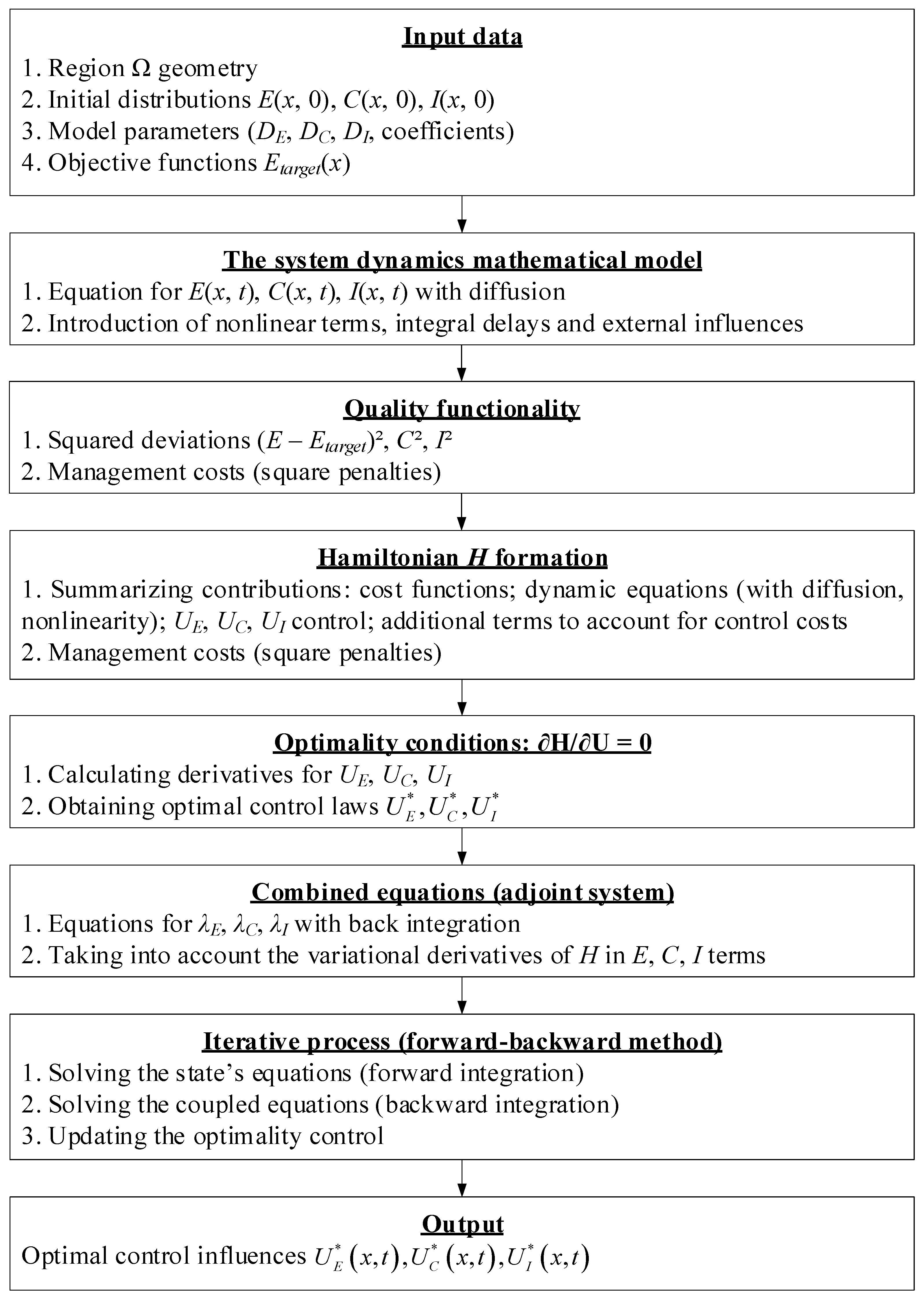
Figure 1. The developed spatial optimisation method’s structural scheme.
Algorithms 18 00523 g001
Figure 2. The developed neural network model for the optimal control problem numerical solution structural scheme.
Algorithms 18 00523 g002
Figure 3. The developed neural network model in the hybrid neural network form for the optimal control problem numerical solution structural scheme.
Algorithms 18 00523 g003
Figure 4. Key parameter diagrams by regions A01, A02, and A03 (the training dataset fragment graphical representation): (a) the “economic activity and population density” chart; (b) the “criminal activity and police resources”; (c) the “risk index over time”.
Algorithms 18 00523 g004
Figure 5. Visual inspection results: (af) the normalised features histograms; (gl) the normalised features QQ-plots.
Algorithms 18 00523 g005aAlgorithms 18 00523 g005b
Figure 6. Correlation analysis results: (a) the “economic activity and population density” chart; (b) The “criminal activity and police resources”.
Algorithms 18 00523 g006
Figure 7. Diagrams of changes in the average significance of E(t), C(t), and I(t) over time.
Algorithms 18 00523 g007
Figure 8. The main variables’ distribution heat maps (show an increased criminal activity localised zone): (a) E(x, t); (b) C(x, t); (c) I(x, t).
Algorithms 18 00523 g008
Figure 9. Diagrams of the control actions UE(t), UC(t), and UI(t) over time.
Algorithms 18 00523 g009
Figure 10. The comparative diagrams (before and after intervention) of criminal activity and risk parameters before and after the intervention.
Algorithms 18 00523 g010
Figure 11. Neural network loss function diagram.
Algorithms 18 00523 g011
Figure 12. Error distribution diagrams.
Algorithms 18 00523 g012
Table 1. Comparative analysis of existing research in the subject area.
Research ApproachAdvantagesDisadvantagesReferences
Mathematical modelling with optimal control methods and neural networksThe comprehensive analysis of socio-economic processes allows for the identification of patterns and the development of recommendations.Full integration with classical dynamic models is not always provided; problems with adapting methods to the social environment and constantly changing conditions are possible.[6,7,8,9]
Advisory solutions for rapid responseThey ensure prompt response from government agencies and help to minimise the negative consequences.There may be insufficient detailing of local features, which leads to the risk of oversimplifying the situation and limiting the accuracy of the proposed measures.[10,11]
The integration of artificial intelligence methods with classical dynamics modelsOpens up new perspectives in solving spatial optimisation problems, taking into account the complex interaction.Requires significant computational resources and adaptation to the area under research specifics, which can complicate the model’s practical application.[12]
Neural network application for numerical problem solving, improving prediction accuracy and cost optimisationAllows for increasing the predictions and optimising management costs accuracy, improving the quality of numerical solutions.Dependence on large amounts of data, the risk of overfitting models, and the difficulty of interpreting the results obtained can reduce the model’s validity without sufficient control.[13,14,15]
Classical logistic growth models and statistical methodsEase of implementation; proven methodological approaches for analysing individual aspects.Lack of comprehensiveness: the relationship between economic development and criminal activity is not taken into account, resulting in a fragmented analysis of problems and limited applicability for crisis management.[16,17]
Reaction–diffusion systemsTaking into account spatial effects, the risks of geographical distribution modelling are possible.Classical models often ignore lagging effects and nonlinear feedback, which can reduce predictive accuracy and limit the ability to adequately respond to rapidly changing processes.[18,19,20]
Logistic equations for the economic and criminological dynamics of simultaneous modellingAn attempt to integrate the two spheres’ dynamics allows for the assessment of the mutual influence of economic growth and criminal activity.The simplified approach often fails to capture the honest feedback between the economy and criminal structures, as the criminal communities’ influence is either taken into account as an external disturbance or ignored altogether, which reduces the model’s reliability in predicting mutual influence.[21,22]
Table 2. Analytical expressions of partial derivatives with respect to E, C, and I from the equations E(t), C(t), and I(t).
EquationPartial Derivative
NameFormulaVariableFormula
Economic activity equation d E d t = α · E · 1 E K
β · E · C + μ · I · E
By E: J 11 = d d E α · E · 1 E K β · E · C + μ · I · E =
= α · 1 2 · E * K β · C * + μ · I *
By C: J 12 = d d C α · E · 1 E K β · E · C + μ · I · E = β · E *
By I: J 13 = d d I α · E · 1 E K β · E · C + μ · I · E = μ · E *
Criminal activity equation d C d t = ρ · C · 1 C γ · E
σ · I + δ · C
Let us write the internal function so as to highlight the dependence on E and C:
ρ · C · 1 C γ · E = ρ · C ρ γ · C 2 E
By E: J 21 = E ρ γ · C 2 E = ρ γ · C 2 E 2 E * , C * = ρ γ · C * 2 E * 2
By C: C ρ · C ρ γ · C 2 E = ρ 2 · ρ · C γ · E .
By adding the term—δ · C, we obtain
J 22 = ρ 2 · ρ · C * γ · E * δ .
By I:J23 = σ.
Table 3. The “forward–backward” iterative process scheme.
Stage NumberStage NameStage Description
1InitialisationThey set the system state initial distributions (economy, crime, risk) and the control actions’ initial approximation.
2Straight pass (“forward”)With current controls, the evolution in time and space is modelled, obtaining predictive trajectories of key indicators.
3Return pass (“back”)Based on the conjugate variables’ final conditions, the corresponding equations are integrated in the opposite direction, forming the deviations’ “value” fields.
4Controls adjustmentUsing the forward and backward pass results, the control actions are updated in order to reduce the target functional, again setting new control laws.
5Convergence checkThe change in the corrections’ control quality or the magnitude is evaluated; when a given criterion is reached, the iterations are terminated, otherwise they return to the forward pass.
Table 4. Developed algorithm for training a neural network.
Stage NumberStage NameDescription
1Data collectionThe neural network’s input is spatial data X(x) = {E(x, t), C(x, t), I(x, t)} at a selected point in time (or a time sequence if a recurrent component or 3D convolutions are used [30,31]).
2Forward passIn the first step, the data is passed through convolutional layers to extract spatial features. Then, fully connected (1 × 1 convolution) layers transform the extracted features into control actions UE(x, t), UC(x, t), and UI(x, t).
3Calculate the loss functionThe loss function L is calculated.
4Error backpropagationBy the backpropagation procedure [32], the filter weights K(l), biases b(l), and matrices W(FC1) and W(FC2) are updated.
5Gradually decrease the loss functionThe model is trained iteratively until convergence, which ensures the optimal control strategy approximation for each point x in the territory.
Table 5. The training dataset fragment.
Region IDTimeEconomic
Activity E
Criminal
Activity C
Risk Index IPopulation DensityPolice
Resources
Youth Unemployment
A0101.550.120.8912000.40.22
A0111.510.181.0412000.40.22
A0121.470.291.2112000.40.22
A0201.200.401.409500.50.35
A0211.180.551.629500.50.35
A0221.150.651.739500.50.35
A0301.700.050.7814000.20.18
A0311.650.070.8514000.20.18
A0321.600.100.9314000.20.18
Table 6. The developed neural network quality assessing results.
Region IDAnalytical ExpressionResulting Value
Accuracy A c c u r a c y = T P + T N T P + T N + F P + F N 0.9907
Precision P r e c i s i o n = T P T P + F P 0.9842
Recall R e c a l l = T P T P + F N 0.9983
F1-score F 1 s c o r e = 2 · P r e c i s i o n · R e c a l l P r e c i s i o n + R e c a l l 0.9912
Average time, minutes64
Average accuracy A ¯ = 1 N · i = 1 N A i 0.9902
Dispersion accuracy D A = 1 N · i = 1 N A i A ¯ 2 0.00000103
Table 7. Comparative analysis results.
The Compared Neural Network ArchitectureComparison
Aims
Comparison MetricResults Obtained
Metric NameDescriptionUsing the Compared Neural NetworkUsing the Developed Neural Network
LSTM Recurrent Network [7]Better modelling of the time dependencies (e.g., risk dynamics over time)MSEThe dynamics prediction error estimation0.01870.0124
Temporal correlation coefficientHow accurately the model captures the temporal structure0.790.91
Convolutional Neural Network for Working with Spatial Distributions [45]The accuracy of identifying geographic risk patterns accuracyIntersection over Union (IoU)Overlap between predicted and actual hotspots0.630.74
Dice coefficientUsed when data is unbalanced0.710.83
Physics-Informed Neural Networks (PINNs) [46]To what extent does the model satisfy the physical–semantic equation (PSE)Residual lossAverage residual between the partial differential equations’ left and right parts0.01510.0093
Conservation scoreHow well the conservation laws are observed in the model0.870.96
GNN (Graph Neural Networks) [47]Using the connections topology between regions (e.g., migration, criminal routes)Node classification accuracyThe city/region node classification accuracy0.97350.9907
F1-scoreRobustness to link noise0.97260.9912
Table 8. The roadmap for future research.
No.Research DirectionObjectiveMethods/InstrumentsPlanned Result
1Introduction of stochastic components into the modelAccounting for random fluctuations and unpredictable social eventsStochastic differential equations (SDEs), Itô-type modelsIncreasing the model’s realism under uncertainty
2Expanding the training data time intervalSeasonal and short-term distortion eliminationLong-term data collection, aggregation methodsIncreasing the neural network’s generalising ability
3Modelling interregional interactionsAccounting for the migration, cross-border crime, and information exchange impactGraph Neural Networks (GNNs), spatial graphsSpatial-network prediction of risk distribution
4The integration of econometric models and expert assessments integrationIncreasing interpretability and linking to real political decisionsBayesian networks, expert systemsHybrid risk management model
5The effectiveness and adaptation to real-life applications evaluationThe model’s validation in pilot regions, and adaptation to the municipal levelReal-world testingRecommendations for implementation in regional management systems
Disclaimer/Publisher’s Note: The statements, opinions and data contained in all publications are solely those of the individual author(s) and contributor(s) and not of MDPI and/or the editor(s). MDPI and/or the editor(s) disclaim responsibility for any injury to people or property resulting from any ideas, methods, instructions or products referred to in the content.