Abstract
In the context of the current global transition toward low-carbon energy, the issue of utilization has become increasingly important. One of the most promising natural targets for sequestration is the terrigenous sedimentary formations found in oil, gas, and coal basins. It is generally assumed that injected into such formations can be stored indefinitely in a stable form. However, the dissolution of into subsurface water leads to a reduction in pH, which may cause partial dissolution of the host formation, altering the structure of the subsurface in the injection zone. This process is relatively slow, potentially unfolding over decades or even centuries, and its long-term consequences require careful investigation through mathematical modeling. The geological formation is treated as a partially soluble porous medium, where the dissolution rate is governed by surface chemical reactions occurring at the pore boundaries. In this study, we present an applied mathematical model that captures the coupled processes of mass transport, surface chemical reactions, and the resulting microscopic changes in the pore structure of the formation. To ensure the model remains grounded in realistic geological conditions, we based it on exploration data characterizing the composition and microstructure of the pore space typical of the Cenomanian suite in northern Western Siberia. The model incorporates the dominant geochemical reactions involving calcium carbonate (calcite, ), characteristic of Cenomanian reservoir rocks. It describes the dissolution of in the pore fluid and the associated evolution of ion concentrations, specifically , , and . The input parameters are derived from experimental data. While the model focuses on calcite-based formations, the algorithm can be adapted to other mineralogies with appropriate modifications to the reaction terms. The simulation domain is defined as a cubic region with a side length of 1 m, representing a fragment of the geological formation with a porosity of 0.33. The pore space is initially filled with a mixture of liquid and water at known saturation levels. The mathematical framework consists of a system of diffusion–reaction equations describing the dissolution of in water and the subsequent mineral dissolution, coupled with a model for surface evolution of the solid phase. This model enables calculation of surface reaction rates within the porous medium and estimates the timescales over which significant changes in pore structure may occur, depending on the relative saturations of water and liquid .
1. Introduction
In the context of the modern trend toward low-carbon energy, the issue of utilization has become increasingly relevant. Currently, there are more than 100 projects worldwide focused on injection and storage in natural reservoirs. Commonly used geological formations for storage include depleted oil and gas reservoirs, aquifers, and underground carbonate and salt layers within sedimentary basins. Particularly promising are terrigenous sedimentary formations within oil, gas, and coal basins. This method of disposal is considered among the most environmentally sustainable.
Due to the presence of geochemical reactions, a 50-year timescale is generally insufficient for complete dissolution [1]. Therefore, mathematical models and numerical simulations are essential tools for analyzing injection and storage processes.
A substantial body of literature is dedicated to the mathematical modeling of injection and storage.
In [2], a hysteresis model is presented that calculates residual brine and saturations, relative permeability, capillary and entry pressures, hydrostatic pressure distributions influenced by brine density, salinity, and mass fraction, as well as geothermal and initial temperature distributions. Only a single cycle of relative permeability hysteresis (drainage and imbibition curves) is modeled. Modern approaches to hysteresis modeling [3,4] are implemented using general-purpose simulators based on unstructured simulation models.
The simulator described in [5] was developed to study storage processes from the wellbore to basin scale. It supports multicomponent, three-phase, three-dimensional fluid flow in heterogeneous porous media. Molar conservation equations are solved using a linearized Newtonian system. Changes in permeability and capillary pressure are considered for different porosity, permeability, and capillary pressure models (e.g., Karman, Labrid, and Fair–Hatch laws).
The leakage assessment simulator in [6] focuses on quantifying fluid distribution and leakage rates in sedimentary systems comprising multiple aquifers, confining beds, and abandoned wells.
A non-isothermal, multiphase, and multicomponent flow simulator is applied to multidimensional reactive water–rock–gas transport in [7].
A detailed simulation of CO2 storage in a realistic 3D reservoir with geological faults and a single injection well is presented in [1]. The results demonstrate stable injection rates over 25 years.
In [8], the author models underground storage involving two-phase flows of and brine in porous media under constant reservoir temperature.
Mineral dissolution processes are often described using thermodynamic equilibrium models where mineral stability depends on pH and ionic activity [9]. However, these simplifications introduce inaccuracies, as mineral dissolution in real systems is largely thermodynamically non-equilibrium and typically irreversible [10].
Geochemical processes such as calcite precipitation and short-term chemical reactions (e.g., carbonic acid formation and organic activity near wells) are often neglected in injection modeling [1,11]. Key modeling objectives usually include modeling advective migration, leakage pathways, porous medium and properties, long-term storage capacity, solubility conditions, and effects of pressure, temperature, and mineral precipitation. Additionally, dissolution lowers pH, potentially leading to rock dissolution and structural changes in the injection zone over extended timescales (decades to centuries), emphasizing the need for detailed modeling. Rock dissolution is governed by surface reactions in a partially soluble porous medium.
Microscale processes have also garnered attention. Some studies investigate the impact of hydrate saturation and morphology on sediment permeability without fully accounting for the dynamic interactions between hydrate structure and pore geometry [12]. Others model permeability as a function of microstructural parameters, assuming idealized pore geometries and hydrate distributions [13]. Experimental insights into hydrate formation and pore behavior are provided using NMR and X-ray CT techniques [14,15,16]. In [17], high-pressure microfluidics are used to study methane hydrate morphology evolution during dissociation.
In [18], depressurization of a storage reservoir is simulated under rock failure scenarios. The authors hypothesize that rock redistribution could form sealing “plugs” that mitigate leakage, although this requires site-specific monitoring.
The study in [19] explores calcite dissolution in deep, dense sandstones using 3D micrometric injection methods. The results show that calcite aggregates of approximately 28 exhibit dissolution behavior strongly influenced by molecular diffusion, solute transport limitations, and aggregate spatial distribution.
In this paper, we present an applied mathematical model that captures a complex set of pore-scale processes, including mass transport, surface chemical reactions, and microstructural evolution of geological formations. To ensure geological relevance, the model incorporates exploration data reflecting the pore composition and structure of the Cenomanian suite in northern Western Siberia. Key geochemical reactions involving calcium carbonate (calcite, ), characteristic of these formations, are included.
The model simulates dissolution in the pore fluid, accounting for changes in , , and ion concentrations. The input parameters are based on experimental data.
The mathematical framework consists of a system of diffusion–reaction equations describing dissolution and mineral interaction at the pore surface, along with a model of the evolving solid interface. It enables estimation of surface reaction rates and the timescales associated with significant structural changes in the porous medium.
Although calibrated for calcite-based systems, the modeling algorithm can be extended to formations with different chemical compositions by modifying the reaction terms accordingly.
2. The Mathematical Model
2.1. An Object for Testing the Model
The Cenomanian formation is considered a key target for geological storage due to its regional extent and stratigraphic consistency. This formation constitutes the principal gas-bearing complex in Western Siberia, located within the upper part of the Maressalinskaya suite of the Albian–Cenomanian subcomplex. The formation was deposited in a continental to shallow marine environment, resulting in a geologically complex lithological structure. The top of the complex is regionally capped by up to 80 m of Turonian marine clays.
To date, more than 70 gas fields have been identified within the Cenomanian formation across Western Siberia. Consequently, the formation is well studied through extensive exploration and production drilling. A large number of core samples have been analyzed, and the composition of reservoir fluids has been comprehensively characterized.
Laboratory analyses of the core material indicate that Cenomanian reservoirs are predominantly composed of interbedded polymictic sandstones and siltstones, exhibiting highly variable reservoir properties. Lithologically, the formation is represented by an uneven alternation of grey siltstones, compacted sands, and calcareous sandstones, with lenticular interbeds and irregular layers of grey to brownish-grey silty clays. The rock fabric is characterized by foliated, lenticular-banded, and occasionally complex and heterogeneous textures. Micaceous laminae, fine carbonaceous detritus, lignified wood fragments, and thin coal seams are frequently observed. The reservoirs consist mainly of weakly consolidated feldspathic–quartz and quartz–feldspathic sandstones and siltstones. The pore space contains both free water and adsorbed water held in diffuse layers.
In the northern part of Western Siberia, the clay content in Cenomanian deposits ranges from 0 to 64%, while the carbonate content ranges from 0 to 16%.
An essential characteristic of the reservoir rocks is their porosity (), defined as the ratio of pore volume to total rock volume. In Cenomanian deposits, porosity values range from 0.22 to 0.44.
According to geological assessments, the gas reserves of the Cenomanian formation are gradually being depleted. Once hydrocarbon production ceases, the depleted reservoirs offer substantial potential for repurposing as geological storage sites. This scenario necessitates comprehensive studies and modeling of storage processes, drawing upon existing data on the geological composition and microscopic structure of the Cenomanian reservoir rocks.
2.2. Micromodel Setup
A cube with an edge of 1 m was selected for modeling. The cube is filled with rock with a porosity of . According to the results of laboratory studies of core samples from the Cenomanian deposit, the effective pore diameter lies in the range of 0.01–0.2 m. These data justify the choice of the computational domain size, since it corresponds to 10–100 times the pore diameter. Note that the volume of one calcite molecule is m3 (see [20] and Section 2.6.2). Thus, the computational domain is, on the one hand, large enough to visualize the chemical processes in the pores and, on the other hand, small enough that the number of grid nodes with a step of m is acceptable for numerical calculations on a personal computer, in particular with the use of distributed computing using CUDA technology.
Based on the pore size data, we assume that the diameters of the rock particles should have similar values, so we represent solid particles in the computational domain volume as balls whose diameters are distributed in the range of 0.01–0.2 m with a step of 0.01 m. We assume that the centers of the spheres are distributed randomly over the volume of the cube, and the distribution by the values of the sphere diameters is considered uniform (see Figure 1a,b), which is consistent with the results of laboratory studies. According to this principle, each node of the computational domain is assigned the value “filled with rock” or “filled with water” since, based on the results of laboratory studies, the pores of the rock of the Cenomanian deposit contain water. During this procedure, we check that the number of nodes “filled with water” is equal to the required porosity, (in this work ), of all the nodes of the computational domain. A detailed description of the algorithm for filling the calculation area is given in Section 3.
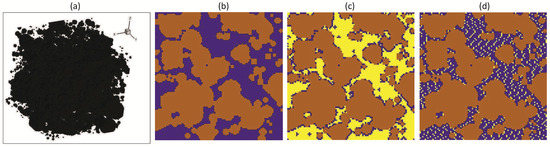
Figure 1.
(a) Three-dimensional illustration of the computational domain. (b) Central cross-section of the computational domain by the OXY plane: brown color—areas filled with solid rock, blue color—pore cavities. (c,d) Central cross-section of the computational domain by the OXY plane with the presence of in the pores: (c) water saturation 0.2 and (d) water saturation 0.8; brown color—areas filled with solid rock, blue color—areas filled with aqueous solution of reaction products, and yellow color—areas filled with .
2.3. The Choice of the Model Equations
The mathematical model describes the physical and chemical processes occurring at the pore scale in the formation after injection. The formation is considered to be a terrigenous aquifer located at depths ranging from 1100 to 1700 m. Based on thermometric measurements conducted in the Cenomanian deposits of Northwestern Siberia, the reservoir temperature is estimated to be in the range of +18 °C to +36 °C, and the pressure varies from 9 to 15 MPa. Under these thermodynamic conditions, carbon dioxide exists in the liquid phase.
A key characteristic of the pore space composition is its water saturation (), defined as the ratio of the volume of pores filled with water to the total pore volume in the region under consideration.
The model incorporates the chemical reactions governing dissolution in water,
and the binding of ions resulting from surface reactions with the soluble fraction of the formation. This is exemplified by the dissolution of calcite:
The model includes equations for the concentrations of the three main types of ions involved in chemical reactions: , , and . (Here, square brackets denote concentrations, following conventional chemical notation.)
In addition, the model incorporates algorithms for defining the computational domain, which simulates the porous medium with injected CO2, as well as the progressive destruction of the formation due to chemical reactions.
The computational domain is a cube with an edge of m, filled with a porous medium with a porosity of . See Figure 1. A uniform grid with nodes
is introduced into the computational domain.
We assume that prior to injection, the pore space was fully saturated with water and that the injection of led to the displacement of water by the liquid phase of . The distribution of fluids within the pores is characterized by saturation, defined as the ratio of the pore volume occupied by a given fluid to the total pore volume in the region of interest. As a result of injection, the water saturation decreased to , while the saturation was established as . Water preferentially wets the pore surfaces, whereas does not [18,21] (Figure 1c,d).
The dissolution reaction of in water, Reaction (1), occurs at the interface of the clusters. Simultaneously, the surface reaction (2), representing the conversion of calcite into water-soluble salts, takes place at the solid pore surface. Both reactions continue until the concentration of ions reaches its maximum permissible value under the specified model conditions within the water-filled domain.
Consequently, the chemical and transport processes within the pore space are governed by reaction–diffusion equations with reactive source terms that incorporate the effects of saturation dynamics. To accurately represent these processes, the model employs equations featuring piecewise linear functions of both concentration and spatial coordinates. These functions exhibit various types of discontinuities, such as sharp transitions at the interfaces between solid rock and clusters, as well as modular-type discontinuities, which together enable the simulation of dissolution up to the saturation threshold of the aqueous solution.
The following equations were used in the model.
The spatial coordinates vary within the domain . Homogeneous Neumann boundary conditions are imposed on all faces of the cube, implying that the inflow of ions across the boundary from the outside is exactly balanced by an equal outflow of ions to the exterior.
The purpose of the modeling is to obtain the distribution of ion concentrations in the pores of the computational domain shown in Figure 1 while maintaining zero concentration of the specified ions inside the solid rock sections. As shown in [22,23,24], systems of equations of this type with discontinuous right-hand sides can have smooth solutions that exhibit sharp transitions from zero to positive values at media discontinuities (in our case, the pore walls). A sufficient condition for the existence of such solutions is a small value of the parameter (). In our model, this smallness indicates that the diffusion of ions into the solid rock is negligibly small.
2.4. The Explanation of the Terms in the Equation System (4)–(6)
- , , and are the maximum possible concentrations of the corresponding ions in solution under the given conditions.In the present study, numerical experiments were conducted using the following value for the limiting concentration of ions [25]. The limiting concentrations of and ions in the system can vary significantly depending on the experimental conditions. Moreover, the molar ratio between these ions may also differ. As an initial approximation, the maximum allowable concentrations of and are assumed to be 0.027 M, corresponding to the approximate solubility level of calcium bicarbonate Ca(HCO3)2 mentioned in the research [26].
- Equation (4) describes the dynamics of the cation concentration in the pore space. In regions occupied by solid rock and the liquid phase of , the equilibrium solution of this equation corresponds to , as captured by the first line of the right-hand side of Equation (4). Therefore, when , the first line effectively models the vanishing cation concentration in both the rock matrix and clusters. In the numerical simulations, we set .
- The second line of the right-hand side of Equation (4) models the variation in the concentration of ions in regions filled with aqueous solution of reaction products. This change arises due to surface reactions associated with the dissolution of and calcite ().
- The term represents a source term for hydrogen cations located at the interface of liquid-phase clusters.
- The multiplier defines the distribution of grid nodes within the computational domain that lie at the interface of clusters. Specifically, this function takes the value 1 at nodes marked as “filled with ” that are adjacent to nodes marked as “filled with water” (namely, filled with aqueous solution of reaction products) and is equal to zero elsewhere. The isolines of this function in the central cross-section of the computational domain in the plane are presented in Figure 2a,b. Regions where the function equals 1 are shown in black, while regions where it equals 0 are shown in blue.
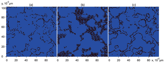 Figure 2. Central cross-section of the computational domain by the OXY plane. Black coloured are the isolines of (a) the surface of dissolution at , (b) the surface of dissolution at , and (c) the surface of pores.
 - The multiplier represents the strength of the cation source and is computed using the following expression:where is the reaction rate constant for the hydration reaction of carbon dioxide: [27]; is the molar mass of ; is a representative concentration of dissolved in water, which relatively quickly predominantly passes into an equilibrium mixture in the form of and , corresponding to the achievement of under given conditions; and .Using these values, we obtain
- The term in the second line of the right-hand side of Equation (4) represents the flux of H+ ions associated with the surface reaction by which calcite molecules are converted into water-soluble compounds at the solid rock interface (i.e., along the pore walls).
- The multiplier defines the distribution of grid nodes in the computational domain that correspond to the pore walls. Specifically, this function takes the value 1 at nodes labeled as “filled with solid rock” that are adjacent to at least one node labeled as “filled with water” (namely, filled with aqueous solution of reaction products) and zero elsewhere. The isolines of this function in the central cross-section of the computational domain in the plane are presented in Figure 2c. Black indicates regions where the function equals 1, and blue indicates regions where it equals 0.
- To determine the value of , we refer to the study by Kaufmann (2007) [28], which investigates the transport of calcium ions into an aqueous solution during surface-mediated calcite dissolution. According to this study, the flux of calcium ions from a solid surface S into a volumewhere is the thickness of the solution layer adjacent to the solid surface, is given bywhere is the rate constant for reaction (2), and is the concentration of hydrogen ions in the surface layer (in M = mol·L−1).To obtain the strength of the volume source in our model, we consider a control volume ofIn the model, the minimum possible width of the near-surface layer is taken as , where h denotes the spatial discretization step defined in Equation (3). For a model porous medium, the average pore surface area within the volume is given bywhere is the total volume of the computational domain, and is the total internal pore surface area in that domain. The volumetric source termis then derived from the balance equationwhich leads to the expressionThe quantity has units of .The algorithm used to compute the value of is presented in Section 3.
- The term represents the net contribution to the cation concentration within the computational domain resulting from their diffusion-driven outflow into the surrounding medium outside the injection zone, as well as inflow from the central region of the injection zone. A quantitative estimate for this term will be provided below. For the time being, it is sufficient to note that its magnitude is several orders smaller than the other terms appearing on the right-hand side of Equation (4).
- The third term on the right-hand side of Equation (4) takes the form of a so-called “modular” discontinuity, which is used to enforce the saturation condition. This condition arises when the concentration of hydrogen cations in the solution reaches the limiting value , corresponding to a saturated solution under the given thermodynamic conditions. In such a case, the state represents an equilibrium configuration of the system, and the concentration remains at this level over an extended period of time.
- The fourth term on the right-hand side of Equation (4) accounts for the cessation of chemical reactions in the case where a saturated solution of ions is formed in the pores, corresponding to the concentration .
- The fourth line on the right-hand side of Equation (5) models the cessation of chemical reactions in the case where a saturated solution of ions has formed within the pore space.
- The term in the second line of the right-hand side of Equation (6) represents the source of ions arising from the dissolution reaction of .
- The terms and have the same interpretation as ; they represent the net effect of ion exchange with the external environment due to diffusion across the boundaries of the computational domain.
2.5. Calculation of the Ion Flow into the External Region Due to Diffusion
The injection zone is not a closed system, and over time, a diffusion-driven outflow of , , and ions occurs into the surrounding region outside the injection area. This outflow originates from regions of the porous medium where the pore space contains saturated solutions of these ions. As a result, chemical reactions involving and the dissolution of the solid matrix can resume. One of the primary objectives of this study is to evaluate the temporal evolution of formation porosity, which requires quantifying the magnitude of these diffusion-driven fluxes.
The diffusion flux represents the number of moles of species i (where i = , , or ) that pass through a unit area perpendicular to the concentration gradient per unit time. It is described by Fick’s law
where is the diffusion coefficient of species i, and is the ion concentration in cm−3. Assuming a cubic computational domain with edge length m and ion concentration (in M) within the pore space, we consider diffusion into an outlying region where ion concentrations are negligibly small.
To obtain an approximate estimate of the transition layer thickness, we used the results from the research [29], which presents modeling of ground displacement in geological porous media in petroleum reservoirs. That study includes a numerically derived model of the reservoir boundary structure. We assume that the widths of boundary (transition) layers in different porous media are likely to be of the same order of magnitude. Therefore, we adopted the transition layer thickness value of km as it is reported in that work.
Therefore, the approximate diffusion flux becomes
The total volumetric flux through all six faces of a cube of side m over 1 s is then
where S is the surface area of one cube face. In the model, diffusion is assumed to occur only from the water-filled part of the pore space. Thus, the diffusion outflow of ions is given by
where m3, is the water saturation, and is the porosity of the formation.
Similarly, the inflow of , , and ions from the central region of the injection zone, where their concentrations are highest, is calculated using the same expression. By summing both fluxes, the net diffusion flow is given by
Substituting into Equation (9) the diffusion coefficients in water, [30], [31] and [32], , km, , and assuming that the water saturation is and the difference is on the order of 0.01, we obtain diffusion flux magnitudes on the order of . These values are 6–7 orders of magnitude smaller than the dominant terms on the right-hand sides of Equations (4)–(6).
This reveals that the model possesses two characteristic timescales: one associated with the rapid establishment of saturated ion concentrations in water-filled pore space (on the order of 1 s) and a second, much slower timescale associated with cumulative diffusion into the surrounding medium, approximately to times longer. Given that there are 86,400 s in a day, the latter can be interpreted as corresponding to a timescale of approximately one day.
The diffusion-driven loss of reaction products results in a change in water saturation, quantified by
where is the total volume of aqueous solution in the pore space, and is the volume of water associated with the removal of dissolved and . This change is given by
where denotes the molar volume of species i (i = , ), and is the time interval over which the diffusion occurs. The following parameter values were used in the numerical implementation: , , , and .
2.6. Modeling Rock Destruction and Boundary Evolution of the Liquid Phase
One of the objectives of this study is to evaluate the temporal evolution of formation porosity. To achieve this, both relevant timescales must be incorporated into the simulation. Additionally, the model must account for the destruction of solid rock and the evolution of the boundaries of clusters.
These processes can only be treated in a discrete manner by updating the configuration of the computational domain at specific time steps, namely, when all material within the grid cells at the interfaces of clusters or solid rock has fully dissolved. In this section, we quantify the amount of and calcite molecules contained in such boundary cells.
Within the numerical implementation, modifications to the pore structure or cluster boundaries are represented as a simultaneous transition of all surface cells from the state of “filled with rock” or “filled with ” to the state of “filled with water” (namely, filled with aqueous solution of reaction products).
2.6.1. Calculation of the Content on Cluster Surfaces
The total volume of the grid cells located on the surface of the clusters within the computational domain can be expressed as
where is the volume of a single grid cell. The number of moles of contained in this volume is given by
where [33] is the density of liquid carbon dioxide, and is its molar mass.
From reactions (1) and (2), it follows that the total number of moles of and ions generated in the domain is equal to the number of moles of dissolved . This relationship will be used in the numerical algorithm (see Section 3): within the model, the boundaries of the clusters are updated when the total number of moles of and ions in the computational domain becomes greater than or equal to x:
2.6.2. Calculation of the Number of Calcite Molecules on Pore Surfaces
A single calcite molecule occupies a volume of [20]. The volume of one grid cell in the computational domain is , which corresponds to approximately calcite molecules per cell.
The total number of calcite molecules located in the grid cells at the surface of the pores is given by
According to reaction (2), converting all the calcite molecules in these surface cells into water-soluble species requires the same number of cations: .
Alternatively, the total number of ions in the computational domain can be computed from the local concentrations:
where is Avogadro’s number.
In the numerical model, the change in the pore surface configuration is triggered when the total number of ions in the computational grid becomes greater than or equal to by a simultaneous transition of all surface cells from the state of “filled with rock” or “filled with ” to the state of “filled with water” (namely, filled with aqueous solution of reaction products).
3. Algorithm for Numerical Implementation of the Model
- Creating a calculation domain
- (1.a)
- Define the computational grid as described in (3) and initialize the grid function with the value , representing cells “filled with ”.
- (1.b)
- Compute the total pore volume as the product of the porosity and the volume of the domain V: .
- (1.c)
- Specify the distribution of particles across size fractions, each represented as spheres with radii , , ranging discretely from to . Ensure that the total volume of these particles does not exceed the pore volume. Determine the number of particles in each fraction.
- (1.d)
- Randomly assign the coordinates of particle centers .
- (1.e)
- Assign the value (“filled with solid rock”) to all grid nodes satisfying the condition:
- (1.f)
- Compute the resulting porosity as , where is the total number of grid nodes, and .
- (1.g)
- If , repeat steps (1.d)–(1.f) for index (smallest particle radius).
- (1.h)
- For all nodes with (“filled with solid rock”), count the number of adjacent nodes with (“filled with ”). Define the grid function accordingly.
- (1.i)
- Compute the total pore surface area as .
- (1.j)
- Assign the value (“filled with water”) to nodes adjacent to “solid rock” cells with (representing smallest pores).
- (1.k)
- Determine the total number of water-filled nodes (in which ). If , assign (“filled with water”) to additional adjacent nodes “filled with solid rock” for which .
- (1.l)
- If , compute . and reset every -th node with to .
- (1.m)
- Repeat steps (1.k)–(1.l) sequentially for until the desired water saturation is reached.
- Initialize the long-cycle counter: .
- Set the initial concentrations of , and ions to zero.
- Increment the long-cycle counter: .
- Repeat step 4 replacing the parameters with scaled parameterswhere is the number of days set in a long time cycle. Continue the computation until the average concentration drops to . Thus, we actually moved in time by days and took into account the amount of reaction products that flowed out during this time beyond the injection area due to diffusion.
- Repeat steps 4 and 5 using the unscaled flow rates computed from (9).
- Check whether the cluster structure remains intact. If condition (11) is satisfied, assign (“filled with water”) to the cluster boundary nodes.
- Check whether the pore surface structure is preserved. If condition (12) is satisfied, assign (“filled with water”) at the pore wall nodes, and recalculate the pore surface area as in steps (1.h) and (1.i).
- Update water saturation according to Formula (10).
- Repeat steps 4–11 until the predefined number of long cycles is completed.
Parameters for the Numerical Implementation
In all the numerical simulations conducted in this study, the following parameters were applied consistently across all computational experiments:
- A spatial grid as defined by Equation (3), with a time step of ;
- The diffusion coefficients , , and (see also Section 2.5);
- ;
- The maximum possible concentrations , , and (see also Section 2.4);
- The functions and , which specify the localization of the reactive interface, which are defined in detail in Section 2.4.
- The value of specified in Equation (7).
- The expression for the diffusion-driven flux , provided in Equation (9).
- Specific parameters such as water saturation and (see Step 7 of the Algorithm) are specified below each figure in Section 4.
For the numerical implementation of the proposed Algorithm, a C++ code was developed using CUDA-based parallel computing technology. The computations were carried out using the method of lines in combination with a one-stage Rosenbrock scheme with a coefficient of , incorporating factorization with respect to the spatial variables.
4. Results and Discussion
Figure 3a–c show the spatial distribution of ion concentrations , , and , respectively, in the central horizontal (OXY) cross-section of the computational domain for a water saturation of . The configuration of solid rock, liquid clusters, and areas filled with aqueous solution of reaction products in this cross-section corresponds to that shown in Figure 1c. These distributions are established within a few seconds and remain nearly unchanged over much longer timescales compared to the equilibration time.
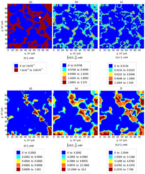
Figure 3.
Equilibrium distribution of reaction product concentrations in pores in the central cross-section of the computational domain by the OXY plane (a–c) at and (d–f) at ; (a,d) ; (b,e) ; and (c,f) . The circular markers identify the spatial locations for which the time-dependent behavior shown in Figure 4 was computed. The spatial profile along which the ion concentration distributions in Figure 5 were extracted is indicated by the yellow line.
The temporal evolution of the ion concentrations , , and at the location marked with a circle in Figure 3a–c is shown in Figure 4a–c, respectively. According to model calculations, equilibration occurs within a few seconds. As seen from the plots, the steady-state concentrations of the ions are relatively low, especially for . This is primarily due to the narrow water-filled regions. The cations produced via reaction (1) at the boundaries of clusters (yellow regions in Figure 1c) hardly diffuse into the -filled domain [34] and instead promptly participate in reaction (2) on the pore walls. As a result, their concentrations in the aqueous phase remain low.
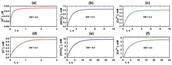
Figure 4.
Temporal evolution of ion concentrations in a representative point of the computational domain for different values of water saturation . Panels (a–c) show the evolution of , , and , respectively, for . Panels (d–f) show the corresponding ion concentration dynamics for . The concentrations are measured at a point indicated by a circle in Figure 3.
Figure 3d–f show the distributions of , , and , respectively, for a water saturation of , with the rock, , and water configuration corresponding to that in Figure 1d. At high water saturation, the reactions occur almost throughout the entire pore space. The fully dissolves in water, resulting in a concentration close to its theoretical maximum. Chemical reactions proceed more intensively than in the case of .
The establishment of ion concentrations , , and at the point marked with a circle in Figure 3d–f is illustrated in Figure 4d–f, respectively, for . Although this state cannot persist indefinitely, it can be regarded as quasi-stationary because its establishment time is significantly shorter than the timescale over which the reaction–diffusion process can be considered steady.
A comparison of the plots in Figure 4a–c for and Figure 4d–f for indicates that the “equilibrium” state is established more rapidly in the case of lower water saturation.
Figure 5 shows the ion concentration distributions as a function of pore geometry patterns for a water saturation of . The spatial profile along which the ion concentration distributions in Figure 5 were extracted is indicated by the yellow line in Figure 3. The peaks in the distributions correspond to the central regions of the pores, as seen in comparison with Figure 3.
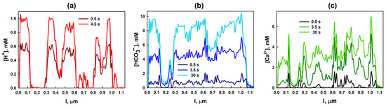
Figure 5.
Spatial distributions of ion concentrations along the yellow line shown in Figure 3, for water saturation : (a) the evolution of concentrations at s and s; (b) the distribution of at s, s, and 30 s; and (c) the corresponding profiles of at the same time intervals.
Figure 5a illustrates that the concentration of hydrogen ions () increases rapidly over time in the central parts of the pores and reaches its equilibrium significantly faster than the concentrations of the other reaction products, and . It is also clearly visible that at early times, the concentrations of and grow more rapidly near the pore walls than in the pore centers. This behavior reflects the surface-controlled nature of the calcite dissolution reaction.
Among the products, ions exhibit the fastest growth, as they are produced simultaneously in both reactions (1) and (2). As time progresses, the concentration peaks shift toward the pore centers due to diffusion, while the concentrations near the pore walls decline. This decline is caused by the depletion of ions near the walls as a result of their consumption in the reaction with calcite. No additional ions can be supplied, as their only source is the dissolution of in water. Under conditions of high water saturation, the completely dissolves within a relatively short time. In our simulation, for the specific case illustrated in Figure 3d–f (in case ), this time was approximately 4.5 s. After this point, the cation concentrations remain essentially constant. As the amount of available decreases, the reaction rates diminish, and the concentrations of and near the pore walls cease to increase as rapidly as they did during the initial stage.
As previously noted, the “steady-state” concentration distribution in the pore space cannot persist indefinitely due to the continuous outflow of reaction products into surrounding regions. According to the estimates presented in Section 2.5, these outflow processes occur approximately seven orders of magnitude more slowly than the process of establishing local equilibrium concentrations. It is not feasible to capture processes occurring on such widely separated timescales using a uniform time step.
For example, with a time step of , the authors’ available computing resources allow for approximately 10,000 iterations per hour, which corresponds to simulating only 10 s of real time. Therefore, to simulate phenomena that take place over months or years, we apply a time-acceleration strategy as described in Steps 6–12 of the Algorithm. Naturally, this approach reduces the accuracy of the simulation results; the longer the prediction horizon, the greater the accumulated error.
Figure 6 illustrates how the Algorithm functions when modeling the transformation of the pore space due to dissolution in a layer with a thickness of one spatial grid step (see Equation (3)). For this illustration, we selected an initial water saturation of because, in this case, the clusters within the pores are relatively large and persist for a sufficiently long time. To “accelerate the time” in simulation, we applied a time-scaling factor , as described in Step 7 of the Algorithm.
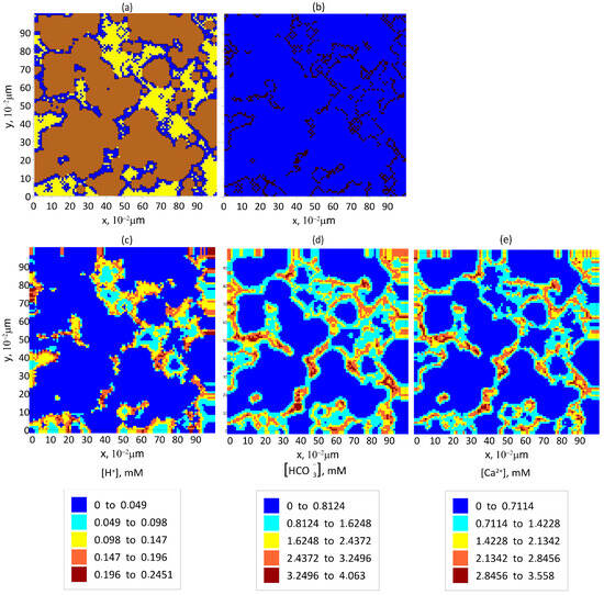
Figure 6.
The pore space filling in and reaction product concentration after approximately 2 years of storing of at a water saturation of in the central cross-section of the computational domain by the OXY plane: (a) the formation: brown color—areas filled with solid rock, blue color—areas filled with aqueous solution of reaction products, and yellow color—areas filled with ; (b) the isolines of the surface of clusters; and (c–e) the equilibrium distribution of reaction product concentrations in pores: (c) , (d) , and (e) .
According to our calculations, after approximately two years of storage, the contained in all the grid cells located at the boundaries of the clusters will have dissolved into the water, causing the cluster boundaries to shift from the pore walls toward the center of the clusters.
The initial pattern distribution corresponding to clusters in the central cross-section of the model cube in the OXY plane is shown in Figure 1c (yellow regions). As the cluster boundaries evolve, the pattern distribution in the same section changes as shown in Figure 6a. The updated isolines of cluster boundaries after the surface layer of has dissolved are depicted in Figure 6b, while the initial isolines are shown in Figure 2a.
Our calculations show that the total surface area of the cluster boundaries increases as a result of this transformation, which in turn enhances the effective interface for dissolution. Consequently, the concentration of ions in the pore space increases. This effect is visible in the comparison between the concentration distributions shown in Figure 3a and Figure 6c.
As a result, the surface reactions are more intense, leading to an increase in the concentrations of both and ions. These effects are evident from comparisons of the respective concentration distributions: for ions in Figure 3b and Figure 6d and for ions in Figure 3c and Figure 6e.
Figure 7 presents a forecast of the porosity change over the course of one year in a region of the reservoir where the water saturation is . To generate this prediction, we employed the time-acceleration factor , as described in Step7 of the Algorithm.
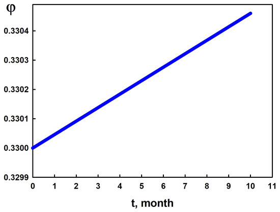
Figure 7.
Simulation of porosity change over 1 year in the region with according to the model.
As shown in Figure 7, the porosity evolves approximately linearly, increasing by about 0.4% per year. Assuming this linear behavior continues, we estimated the time required to completely dissolve a layer of rock with a thickness equal to one spatial grid step (see (3)) in the region of the reservoir where . To perform this estimate, we reduced the destruction threshold in condition (12) (by a factor of 1000). As a result, the destruction criterion took the following form:
Then, we executed the Algorithm again using the same time-scaling factor .
According to our calculations, the time required to dissolve the specified rock layer is approximately 1000 years. The resulting change in the spatial distribution of the solid rock—represented by binary patterns in the central cross-section of the computational domain (OXY plane)—compared to the initial state (see Figure 1b) is shown in Figure 8a. It should be noted that this estimate is relatively coarse. A more accurate prediction of the reservoir condition over periods exceeding 10 years would require further refinement of geological, physical, and chemical system parameters, which is a subject for future research.
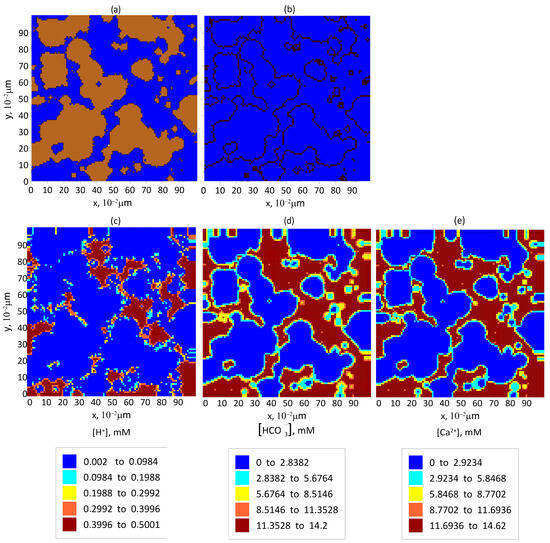
Figure 8.
The pore space filling in and reaction product concentration after 1000 years of storing of at a water saturation of in the central cross-section of the computational domain by the OXY plane: (a) the formation: brown color—areas filled with solid rock and blue color—areas filled with aqueous solution of reaction products; (b) the isolines of the pore surface; and (c–e) the equilibrium distribution of the reaction product concentrations in the pores: (c) , (d) , and (e) .
Nevertheless, the resulting distributions of the reaction products are physically reasonable. The concentration of ions in the central section, shown in Figure 8c, is approximately half that in Figure 3d, which corresponds to the case without rock dissolution. This is due to the fact that the only source of ions in this scenario is the diffusive flux from the central part of the injection zone. The elevated calcium ion concentration shown in Figure 8d, compared to Figure 3e, is explained by the substantial amount of dissolved rock. The comparable concentrations of and ions in Figure 8e,d, respectively, indicate that the supply of these ions primarily results from surface reactions involving the dissolution of calcite.
Based on the graph in Figure 7, a 10% increase in porosity within the transition layer is projected to occur over approximately 30 years. This duration can be considered a rough estimate of the time required for the transition layer to advance by a distance equal to its own thickness, i.e., approximately 0.5 km. According to the model calculations, in the region where the water saturation is , the porosity remains nearly constant over time. Therefore, in long-term predictions of solid rock degradation, the primary mechanism will be the gradual displacement of the transition layer boundary.
5. Conclusions
In this work, we presented a mathematical model for simulating storage in underground geological formations, capturing the microscale processes associated with rock–fluid interactions. A detailed algorithm was developed to account for changes in pore structure due to rock dissolution during numerical simulations. Additionally, we proposed a strategy to incorporate two significantly different timescales in the modeling of long-term rock degradation.
The model enables the following:
- The estimation of changes in formation porosity;
- The assessment of the volumetric sink capacity due to diffusion in non-injection regions, which can be integrated into macroscopic models of storage;
- The prediction of the evolution of the transition layer (i.e., the zone in which the saturation of the reaction products decreases from maximum to zero) within the injection area.
The model has certain limitations:
- Accurate concentration distributions can only be obtained when the diffusion coefficients in Equations (4)–(6) are sufficiently small [23,24]. Physically, this implies that there is negligible diffusion of reaction products into the solid matrix or into the CO2 liquid-phase clusters. In numerical practice, such small diffusion terms serve as artificial viscosity.
- The model assumes constant storage conditions and does not account for precipitation via the reverse reaction of Equation (2).
- The microscale model assumes a fixed spatial distribution of water saturation. Therefore, the model can be used to evaluate the state of the rock at a specific point within the storage reservoir, but it does not provide a macroscopic spatial distribution across the reservoir domain as a whole.
The primary goal of this study was to test the mathematical model. For this purpose, the model was calibrated using the typical composition of the Cenomanian formation and the chemical reactions characteristic of such lithology. The model can be further adapted to account for alternative geological features and varying storage conditions. The obtained results describing the long-term evolution of the storage boundary can be incorporated into macroscopic storage models for large-scale assessment and planning.
Author Contributions
Conceptualization, N.L. and P.L. and A.S.; methodology, P.L.; software, N.L.; validation, D.E.; formal analysis, D.E.; writing—original draft preparation, N.L. and A.S.; project administration, A.S. All authors have read and agreed to the published version of the manuscript.
Funding
This research was funded by the Russian Science Foundation grant number 23-11-00069.
Data Availability Statement
Data is contained within the article. Further inquiries can be directed to the corresponding author.
Conflicts of Interest
The authors declare no conflicts of interest.
Correction Statement
This article has been republished with a minor correction to the Data Availability Statement. This change does not affect the scientific content of the article.
References
- Class, H.; Ebigbo, A.; Helmig, R.; Dahle, H.K.; Nordbotten, J.M.; Celia, M.A.; Audigane, P.; Darcis, M.; Ennis-King, J.; Fan, Y.; et al. A benchmark study on problems related to CO2 storage in geologic formations. Comput. Geosci. 2009, 13, 409–434. [Google Scholar] [CrossRef]
- Land, C.S. Calculation of imbibition relative permeabilities for two- and three-phase flow from rock properties. Soc. Pet. Eng. J. 1968, 8, 149–156. [Google Scholar] [CrossRef]
- Fan, Y. Development of CO2 Sequestration Modeling Capabilities in Stanford General Purpose Research Simulator. Master’s Thesis, Stanford University, Stanford, CA, USA, 2006. [Google Scholar]
- Jiang, Y. Techniques for Modeling Complex Reservoirs and Advanced Wells. Ph.D. Thesis, Stanford University, Stanford, CA, USA, 2007. [Google Scholar]
- Trenty, L.; Michel, A.; Tillier, E.; Le Gallo, Y. A sequential splitting strategy for CO2 storage modelling. In Proceedings of the 10th European Conference on the Mathematics of Oil Recovery, Amsterdam, The Netherlands, 4–7 September 2006. [Google Scholar]
- Nordbotten, J.M.; Kavetski, D.; Celia, M.A.; Bachu, S. A semi-analytical model estimating leakage associated with CO2 storage in large-scale multi-layered geological systems with multiple leaky wells. Environ. Sci. Technol. 2009, 43, 743. [Google Scholar] [CrossRef]
- Sbai, M.A.; Azaroual, M. A numerical model for miscible displacement of multi-component reactive species. Dev. Water Sci. 2004, 55, 849–859. [Google Scholar] [CrossRef]
- Afanasyev, A.; Kempkab, T.; Kühnb, M.; Melnik, O. Validation of the MUFITS reservoir simulator against standard CO2 storage benchmarks and history-matched models of the Ketzin pilot site. Energy Procedia 2016, 97, 395–402. [Google Scholar] [CrossRef]
- Loughnan, F.C. Chemical Weathering of Silicate Minerals; American Elsevier Publishing Company: New York, NY, USA, 1969. [Google Scholar]
- Sokolova, T.A. Decomposition of clay minerals in model experiments and in soils: Possible mechanisms, rates, and diagnostics (analysis of literature). Eurasian Soil Sci. 2013, 46, 182–197. [Google Scholar] [CrossRef]
- Ebigbo, A.; Class, H.; Helmig, R. CO2 leakage through an abandoned well: Problem-oriented benchmarks. Comput. Geosci. 2007, 11, 103–115. [Google Scholar] [CrossRef]
- Wu, P.; Li, Y.; Wang, L.; Sun, X.; Wu, D.; He, Y.; Li, Q.; Song, Y. Hydrate-bearing sediment of the South China Sea: Microstructure and mechanical characteristics. Eng. Geol. 2022, 307, 106782. [Google Scholar] [CrossRef]
- Wu, Y.; Tahmasebi, P.; Lin, C.; Dong, C. Process-based and dynamic 2D modeling of shale samples: Considering the geology and pore-system evolution. Int. J. Coal Geol. 2020, 218, 103368. [Google Scholar] [CrossRef]
- Kumar, A.; Maini, B.; Bishnoi, P.R.; Clarke, M.; Zatsepina, O.; Srinivasan, S. Experimental determination of permeability in the presence of hydrates and its effect on the dissociation characteristics of gas hydrates in porous media. J. Pet. Sci. Eng. 2010, 70, 114–122. [Google Scholar] [CrossRef]
- Kou, X.; Feng, J.; Li, X.; Wang, Y.; Chen, Z. Visualization of interactions between depressurization-induced hydrate decomposition and heat/mass transfer. Energy 2022, 239, 122230. [Google Scholar] [CrossRef]
- Xiao, C.; Li, X.; Lv, Q.; Yu, Y.; Yu, J.; Li, G.; Shen, P. Experimental measurement and clustered equal diameter particle model of permeability with methane hydrate in glass beads. Fuel 2022, 320, 123924. [Google Scholar] [CrossRef]
- Zhang, J.; Song, Z.; Zhou, K.; Li, Q.; Jiao, H.; Yin, Z. Pore-Scale Analysis of the Permeability and Effective Thermal Conductivity of Hydrate-Bearing Sediments Based on a High-Pressure Microfluidics Approach. Energy Fuels 2024, 38, 22192–22204. [Google Scholar] [CrossRef]
- Xu, R.N.; Li, R.; Ma, J.; He, D.; Jiang, P.X. Effect of Mineral Dissolution/Precipitation and CO2 Exsolution on CO2 transport in Geological Carbon Storage. Accounts Chem. Res. 2017, 50, 2056–2066. [Google Scholar] [CrossRef]
- Wang, W.; Zhang, X.; Mao, C.; Hao, Z.; Liang, Z.; Wang, D.W.; Zhu, Y. The dissolution mechanism of calcite and its impact on CO2 sequestration in deep-water sandstone during CO2 flooding: A case study in the Chang 7 member, Ordos Basin, China. Mar. Pet. Geol. 2025, 182, 107566. [Google Scholar] [CrossRef]
- The Materials Project. Available online: https://next-gen.materialsproject.org/ (accessed on 6 April 2025).
- Bachu, S.; Bonijoly, D.; Bradshaw, J.; Burruss, R.; Holloway, S.; Christensen, N.P.; Mathiassen, O.M. CO2 storage capacity estimation: Methodology and gaps. Int. J. Greenh. Gas Control 2007, 1, 430–443. [Google Scholar] [CrossRef]
- Pavlenko, V.N.; Ul’yanova, O.V. Method of Upper and Lower Solutions for Parabolic-Type Equations with Discontinuous Nonlinearities. Differ. Equ. 2002, 38, 520–527. [Google Scholar] [CrossRef]
- Nefedov, N.; Tishchenko, B.; Levashova, N. An Algorithm for Construction of the Asymptotic Approximation of a Stable Stationary Solution to a Diffusion Equation System with a Discontinuous Source Function. Algorithms 2023, 16, 359. [Google Scholar] [CrossRef]
- Tishchenko, B.V. Existence of solutions of a system of two ordinary differential equations with a modular–cubic type nonlinearity. Theor. Math. Phys. 2023, 215, 735–750. [Google Scholar] [CrossRef]
- Haghi, R.K.; Chapoy, A.; Peirera, L.M.C.; Yang, J.H.; Tohidi, B. pH of CO2 saturated water and CO2 saturated brines: Experimental measurements and modelling. Int. J. Greenh. Gas Control 2017, 66, 190–203. [Google Scholar] [CrossRef]
- Zhao, D.F.; Buchholz, A.; Mentel, T.F.; Müller, K.-P.; Borchardt, J.; Kiendler-Scharr, A.; Spindler, C.; Tillmann, R.; Trimborn, A.; Zhu, T.; et al. Novel method of generation of Ca(HCO3)2 and CaCO3 aerosols and first determination of hygroscopic and cloud condensation nuclei activation properties. Atmos. Chem. Phys. 2010, 10, 8601–8616. [Google Scholar] [CrossRef]
- Falkowski, P.G.; Raven, J.A. Aquatic Photosynthesis; Princeton University Pressp.: Princeton, NJ, USA, 2007; p. 160. [Google Scholar]
- Kaufmann, G.; Dreybrodt, W. Calcite dissolution kinetics in the system CaCO3 − H2O − CO2 at high undersaturation. Geochim. Cosmochim. Acta 2007, 71, 1398–1410. [Google Scholar] [CrossRef]
- Afanasyev, A.; Utkin, I. Modelling ground displacement and gravity changes with the MUFITS simulator. Adv. Geosci. 2020, 54, 89–98. [Google Scholar] [CrossRef]
- Yan, X.; Delgado, M.; Aubry, J.; Gribelin, O.; Stocco, A.; Boisson-Da Cruz, F.; Bernard, J.; Ganachaud, F. Central Role of Bicarbonate Anionsin Charging Water/Hydrophobic Interfaces. J. Phys. Chem. Lett. 2018, 9, 96–103. [Google Scholar] [CrossRef] [PubMed]
- Elovikova, T.M. Analiz vliyaniya lechebno-profilakticheskoj zubnoj pasty s ehkstraktami trav na sostoyanie polosti rta u pacientov s gingivitom. Probl. Stomatol. 2015, 2, 5–9. (In Russian) [Google Scholar]
- Schuszter, G.; Gehér-Herczegh, T.; Szűcs, Á; Tóth, Á; Horváth, D. Determination of the diffusion coefficient of hydrogenion in hydrogels. Phys. Chem. Chem. Phys. 2017, 19, 12136–12143. [Google Scholar] [CrossRef]
- Lee, J.; Lee, J.I.; Yoon, H.J.; Cha, J.E. Supercritical Carbon Dioxide turbomachinery design for water-cooled Small Modular Reactor application. Nucl. Eng. Des. 2014, 270, 76–89. [Google Scholar] [CrossRef]
- Stone, H.W. Solubility of Water in Liquid Carbon Dioxide. Ind. Eng. Chem. 1943, 35, 1284–1286. [Google Scholar] [CrossRef]
Disclaimer/Publisher’s Note: The statements, opinions and data contained in all publications are solely those of the individual author(s) and contributor(s) and not of MDPI and/or the editor(s). MDPI and/or the editor(s) disclaim responsibility for any injury to people or property resulting from any ideas, methods, instructions or products referred to in the content. |
© 2025 by the authors. Licensee MDPI, Basel, Switzerland. This article is an open access article distributed under the terms and conditions of the Creative Commons Attribution (CC BY) license (https://creativecommons.org/licenses/by/4.0/).