EpiInfer: A Non-Markovian Method and System to Forecast Infection Rates in Epidemics

Abstract

Consider an evolving epidemic in which each person is either (S) susceptible and healthy; (E) exposed, contagious but asymptomatic; (I) infected, symptomatic, and quarantined; or (R) recovered, healthy, and susceptible. The inference problem, given (i) who is showing symptoms (I) and who is not (S, E, R) and (ii) the distribution of meetings among people each day, is to predict the number of infected people (state I) in future days (e.g., 1 through 20 days out into the future) for the purpose of planning resources (e.g., needles, medicine, staffing) and policy responses (e.g., masking). Each prediction horizon has different uses. For example, staffing may require forecasts of only a few days, while logistics (i.e., which supplies to order) may require a two- or three-week horizon. Our algorithm and system EpiInfer is a non-Markovian approach to forecasting infection rates. It is non-Markovian because it looks at infection rates over the past several days in order to make predictions about the future. In addition, it makes use of the following information: (i) the distribution of the number of meetings per person and (ii) the transition probabilities between states and uses those estimates to forecast future infection rates. In both simulated and real data, EpiInfer performs better than the standard (in epidemiology) differential equation approaches as well as general-purpose neural network approaches. Compared to ARIMA, EpiInfer is better starting with 6-day forecasts, while ARIMA is better for shorter forecast horizons. In fact, our operational recommendation would be to use ARIMA (1,1,1) for short predictions (5 days or less) and then EpiInfer thereafter. Doing so would reduce relative Root Mean Squared Error (RMSE) over any state of the art method by up to a factor of 4. Predictions of this accuracy could be useful for people, supply, and policy planning.

1. Introduction

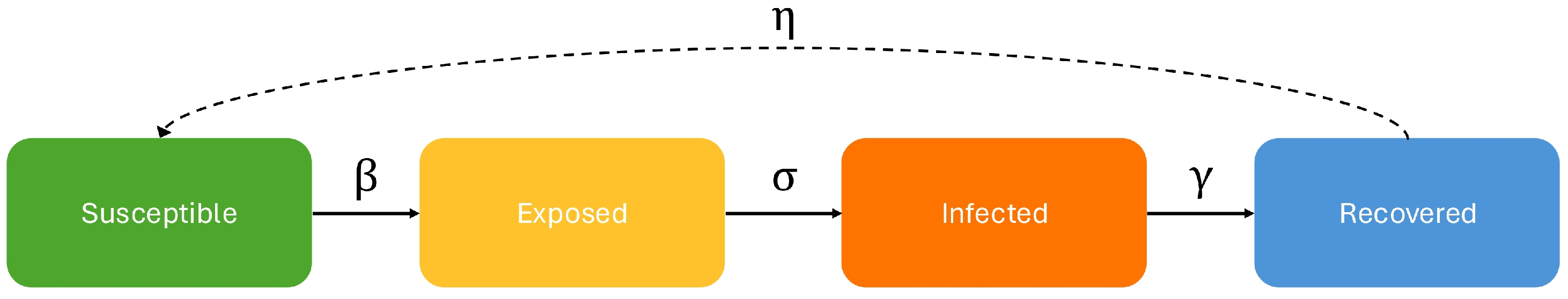
Kermark et al. [1] introduced compartmental epidemiological models such as the Susceptible–Infected–Recovered model in which an agent is either Susceptible (healthy) or Infected (symptomatic and contagious) or Recovered (healthy and with partial immunity). By adding the Exposed compartment (asymptomatic and contagious), this model can be extended to the SEIRS model which characterizes most epidemics in which people can be contagious but not symptomatic. Understanding the evolution of an epidemic requires knowing the transition probabilities between these states, a process called calibration. The relationship between the states and parameters can be seen in Figure 1.

Various surveys have compared calibration methods. For instance, the survey conducted by Gupta et al. [2] used EpiPolicy [3] to compare these methods through simulations. The EpiPolicy simulator allows users to include features such as sub-population groups, facilities, population mobility, vaccination, hospitalization, mask-wearing, border closures, lockdowns, and school closures. The survey concluded that the best algorithm depends on the type of model and data, but there are certain algorithms such as Levenberg–Marquardt (least squares) that tend to perform well in many different cases.

The overall process of estimating infection rates can be broken down into two tasks: (i) inferring transition parameters between states and then (ii) using those parameter values to infer infection rates.

Some methods for both tasks make use of contact tracing information which gives how many people each person meets and whom they meet. Because such information is rarely available in quantity, EpiInfer only makes use of the distribution (and even only the mean of the distribution) of how many people each person meets (but not whom).

This paper presents and evaluates a new algorithm called EpiInfer as well as some variants. The paper’s contributions can be divided into a few parts:

• Our algorithm EpiInfer consists of two components EpiInfer-core and an outer-loop algorithm ContinuousCalibrate that iterates over various hyperparameter settings in calling EpiInfer-core.
• The non-Markovian algorithm EpiInfer-core projects future infection rates starting at any day d by considering (i) the number of newly infected patients in a few days before d, (ii) some information about the meeting distribution of people, and (iii) transition probabilities between the Susceptible (S), Exposed (E), and Infected (I) states.
• Because the transition probabilities are not known at the beginning of an epidemic, ContinuousCalibrate recomputes the transition probabilities at each day by calling EpiInfer-core on previous data and various parameter settings. This dynamic setting of parameters follows the spirit of [4].
• We show how using multiple locales can help ContinuousCalibrate improve the estimation of transition parameters and thereby improve infection prediction, especially early in an epidemic.
• Though EpiInfer is most accurate when given a full meeting distribution, we show that using just the mean number of meetings per person is often enough.
• Our experiments show that the two-component EpiInfer predicts better than (Markovian) Differential Equation models and LSTMs (as well as other neural network models) regardless of the forecast window. ARIMA is more accurate than EpiInfer for short-term predictions, but EpiInfer is more accurate than ARIMA starting at 7 days.

2. Related Work

We divide the related work into the two tasks of calibration and prediction of infection.

2.1. Calibration

Algorithms for the calibration of differential equation models can be separated into two major groups: gradient-based methods and gradient-free methods. Here, we review the major algorithms from each group.

2.1.1. Gradient-Based

Least-squares minimization using the Trust Region Reflective method [5] optimizes parameters by constraining updates to stay within a predefined distance (the “trust region”) from the current best guess. It computes the Jacobian matrix and determines the size of the trust region. The parameters are updated iteratively so that the objective function is minimized.

Truncated Newton [6] computes a partial Hessian matrix to reduce computational complexity. It uses this truncated matrix to update the search direction, and a line search to determine the step size along this direction. BFGS [7] is an algorithm that avoids directly computing the actual Hessian matrix of the objective function by iteratively approximating it. After each iteration and update to the approximation of the matrix, this new information is used to determine the step size and the search direction. There is also a limited memory version of this method that stores only a portion of past information to approximate the Hessian matrix [2]. The Levenberg–Marquardt [4] algorithm iteratively updates the parameters of a model. It works by reducing the difference between the predicted data of the compartmental model based on the current parameter estimation and the real data across all compartments available in the current epidemic dataset that is being considered. It starts with an initial guess of the parameters and then updates them using gradient descent.

2.1.2. Gradient-Free

Powell’s method [8] finds the minimum of a function without calculating derivatives. This method iteratively updates search vectors until there are no significant improvements.

Differential Evolution [9] is a heuristic for global optimization over discontinuous spaces or when gradients are unreliable. This method proposes a set of candidate solutions and modifies them discretely, then does recombination in the spirit of genetic algorithms.

Adaptive Memory Programming (AMP) for Global Optimization [10] is an algorithm for global optimization on non-convex problems. It works by maintaining a set of the best solutions found so far, which is called the memory. The search begins with a randomly generated population of solutions that are evaluated with an objective function, and the best ones are chosen to form the initial memory. After every iteration, a new population is created by combining the current population with the memory. The new solutions that are the best according to the objective function (e.g., the estimate of population in each compartment) are added to the memory, and they replace the worst solutions from the memory.

The basin-hopping algorithm [11] tries to find a global minimum even though there are many local minima. It starts from an initial point and then moves randomly to nearby points using an approach close to simulated annealing [12]. After that, it starts looking for nearby points that are lower cost and moving to them. At times, it makes a random move for exploration purposes. This keeps happening until there are not any lower points or a certain stopping condition occurs.

Dual Annealing [13] combines simulated annealing with genetic algorithms. It uses two optimizations at the same time, one conducted locally and one globally. Local optimization uses standard optimization techniques. The global optimization is carried out by moving from a state to one of its neighboring states, where each transition could happen with a certain probability.

2.2. Models That Use Information About Meetings

The above approaches try to calibrate transition likelihoods knowing how many people are in each compartment, but do not use information about the interaction among people. Because information about person-to-person interactions is often available, e.g., through surveys, several methods use that information.

Predicting infection trends can benefit greatly from knowing about the interaction among people for human epidemics but, in general, for agents (e.g., for animal epidemics). The best case from the point of view of analysis occurs when full meeting information is known (who meets whom), such as in contact tracing-based scenarios, but such data greatly infringes on privacy. When only meeting survey information is available (how many people do each person meet), meeting distribution-based models make sense.

2.2.1. Agent-Based Models

Agent-based models trace each interaction between individual agents (e.g., people for human epidemics). Hunter et al. [14] propose a hybrid model combining agent-based simulations and equation-based methods. They showed that the agent-based models helped to make predictions at low infection levels, while the equation-level predictions were computationally more efficient for high infection levels.

Eubank et al. [15] also employ an agent-based approach, utilizing dynamic bipartite graphs generated from urban traffic simulations based on real-world mobility data, to model the spread of infectious diseases. Their findings suggest that human contact networks show small-world properties, because people interact in their own friend groups.

Venkatramanan et al. [16] use a hybrid modeling approach that combines agent-based modeling with Bayesian calibration and simulation optimization (Nelder–Mead) to study epidemics. Bayesian calibration uses response surfaces to estimate parameter distributions and align simulations with observed epidemic data, while Nelder–Mead optimization minimizes the error between simulated and observed curves. Their study shows that data-driven agent-based models can forecast infectious disease outbreaks effectively by integrating diverse data sources.

2.2.2. Contact Tracing-Based Models

Contact tracing-based models offer detailed person-to-person analysis by identifying who interacted with whom during each encounter. Muntoni et al. [17] combine agent-based modeling to simulate epidemic dynamics with probabilistic contact tracing with Belief Propagation and Simple Mean Field algorithms to identify superspreaders and reconstruct transmission pathways. They find that probabilistic contact tracing methods improve epidemic containment by efficiently detecting superspreaders, enhancing backward and multi-step tracing, and reducing social and diagnostic costs compared to traditional contact tracing approaches.

Kim et al. [18] propose a multi-hop contact tracing strategy, which identifies and monitors direct contacts of an infected individual but also traces secondary, tertiary, and further levels of contacts within the transmission network. By using the Microscopic Markov Chain Approach (MMCA), the model simulates disease transmission dynamics and evaluates the effectiveness of multi-hop tracing in controlling outbreaks. Their study shows that multi-hop contact tracing enhances epidemic containment, and their proposed mathematical framework enables faster and more scalable computation compared to traditional Monte Carlo simulations.

Tuschhoff and Kennedy [19] rely on contact tracing data to detect and estimate heterogeneity in susceptibility. Likelihood ratio tests are used to evaluate the fit of competing susceptibility models, and maximum likelihood estimation (MLE) is included to estimate model parameters. They conclude that contact tracing data alone are sufficient to detect and quantify the heterogeneity in susceptibility, allowing early identification of differences in infection likelihood among individuals, which leads to improvements in epidemic modeling and public health interventions.

Hens et al. [20] propose what they call a Next-Generation Matrix (NGM) framework which combines contact matrices, derived from diary-based contact survey data, with previously known epidemiological parameters such as the transmission probability and the duration of infectiousness. The largest eigenvalue of the NGM represents the basic reproduction number. The study enhances the estimation of the basic reproduction number by incorporating professional contact data and refining age-specific interaction patterns.

2.3. Meeting Distribution-Based Models

Unlike agent-based and contact tracing-based models that focus on individual-level contact data, meeting distribution-based models rely on population-level interaction patterns. Veneti et al. [21] estimate age-stratified contact matrices—the average number of daily contacts between individuals of different age groups—and calculate reductions in the basic reproduction number using the next-generation method. Their study showed social distancing measures during COVID-19 reduced the basic reproduction number by 25% compared to what it would have been had there been no social distancing.

Mistry et al. [22] construct age-stratified contact matrices (saying how likely persons of different age groups would meet each other in a variety of locales) using socio-demographic data and POLYMOD surveys. They offer a case study of estimating the reproduction number of the H1N1 2009 epidemic in a variety of countries. They show that taking into account the variability in the distribution of contacts gives greater accuracy compared to a uniform mixing model.

Boyer et al. [23] develop a theoretical transmission model using empirical gathering size data from the BBC Pandemic and Copenhagen Networks Study (CNS). Their transmission model calculates the expected number of new infections at a certain gathering size based on transmission probability and population proportions of susceptible and infectious individuals. Their study shows that for COVID-19, gatherings would have to be severely restricted in size to prevent epidemic spread.

Munday et al. [24] construct an age-specific forecasting framework and apply it to two age-stratified time-series data; the first one is the incidence of SARS-CoV-2 infection estimated from the national infection and antibody prevalence survey, and the second one is the reported cases based on the UK COVID-19 dashboard. They predict new infections by using real-time contact patterns combined with a semi-mechanistic model that estimates how people of different ages interact and transmit the virus, accounting for changes in immunity, vaccination, and infection rates over time. Their study finds that incorporating age interaction can improve infection predictions, particularly in children and older adults, and the social contact data informed model performs the best in the short term (between 2–4 weeks) and the winter months in 2020–2021.

Franco et al. [25] present a method to analyze age-specific variations in transmission parameters associated with susceptibility and infectiousness to SARS-CoV-2 infection. They combine social contact data with the next-generation principle to estimate relative infection rates across different age groups. Their findings indicate that children, especially preschool-aged young children, have about half the susceptibility of adults. Although this study does not explicitly track individual-level meetings, it estimates contact distributions using diary-based social contact data, which serve as an aggregate representation of meeting patterns across age groups.

An important insight from the above excellent work is that knowing as much information as possible about meetings is helpful. Practically speaking, however, we find that basically no contact tracing data is available or, if it is, then only in small quantities. What is available is survey data indicating how many people each person meets.

3. Materials and Methods

EpiInfer assumes that the following is given: the total population, the number of symptomatic individuals (state I) over time, and an estimate of the number of daily contacts per asymptomatic individual (though not who meets whom).

Because we are not using a differential equation model, we are not trying to estimate the parameters of such a model (e.g., $\beta$ and $\sigma$). Instead, we try to estimate (and then use) three parameters.

• $p_1$ the probability that a person in susceptible state S will transition to state E after encountering one person in an asymptomatic but contagious state E.
• $p_2$ the probability that a person in state E will transition to symptomatic state I.
• $inc$ the number of days of incubation between the time a person enters state E and they enter state I.

To explain our strategy, we will start in Section 3.1 by explaining the EpiInfer-core method to infer infections given the meeting distribution and guesses of $p_1$, $p_2$, and $inc$. Next, in Section 3.2, we describe ContinuousCalibrate, a grid/binary search method to find those parameter values: for each $p_2$ between 0.1 and 1 in 0.1 increments, perform binary search on $p_1$ to find a set of $p_1$ and $p_2$ values for which EpiInfer-core yields the smallest error for the last day. Finally, in Section 9.1, we describe an approach to use multiple more or less isolated locales to infer these parameters better.

3.1. EpiInfer-Core: Estimating Infection Rates from Basic Parameters

For given transition probabilities $p_1$, $p_2$, average incubation period $inc$, and statistical information in the form of a distribution of the number of people each person meets each day, the algorithm has several components to predict how many people will be infected on a given day d, given the number of newly infected on previous days.

Anyone who entered the infected/symptomatic state I at time $d-i$, for some $i\le inc$, must have already been in the Exposed state at the start of time $d-inc$. Thus, the probability $palreadyex{p}_{d-inc}$ that an asymptomatic person is already in the exposed state at the start of time $d-inc$ is

$$palreadyex{p}_{d-inc}=(\sum _{i=1}^{inc}NewInf(d-i))/(p_2·asymptomatic(d-inc))$$

(1)

where $asymptomatic(d-inc)$ is the number who were asymptomatic at time $d-inc$ (i.e., not in state I) and $NewInf(d-i)$ is the number of people who enter the infected state on day $d-i$. Thus, the probability $palreadyex{p}_{d-inc}$ is proportional to the number who became infected since $d-inc$ and inversely proportional to the whole population of the asymptomatic ones at $d-inc$. The $p_2$ divisor reflects the fact that not all who become exposed subsequently become infected, so if $p_2$ is small, then few who become exposed later become infected.

So, if a person y meets $n_y$ people at time $d-inc$, then y will meet approximately $n_y·$$palreadyex{p}_{d-inc}$ already exposed people. As a consequence, the probability that an asymptotic person y becomes exposed at $d-inc$ is

$$pnewexposed(d-inc,y)=1-{(1-p_1)}^{n_y·palreadyex{p}_{d-inc}}.$$

(2)

To avoid double-counting the number of exposed people, we want to exclude those people who are already exposed at day $d-inc$. There are ${\sum }_{i=1}^{inc}NewInf(d-i)/p_2$ people who are already exposed as of that day.

$asymptomaticNotEx$ denotes those who are asymptomatic, not exposed, but who could be exposed. Therefore,

$$\begin{array}{c}asymptomaticNotEx(d-inc)=asymptomatic(d-inc)\hfill \\ -(\sum _{i=1}^{inc}NewInf(d-i)/p_2)-\left(recovered(d-inc)\right).\hfill \end{array}$$

(3)

The last term reflects the fact that recovered people have immunity for a certain period of time. So, we subtract the number of recovered people at time $d-inc$ from those who could be exposed.

So, the expected number of newly exposed people at $d-inc$ is

$$NewExposed(d-inc)=\sum _{yinasymptomaticNotEx(d-inc)}pnewexposed(d-inc,y)$$

(4)

where $pnewexposed(d-inc,y)$ is given by Equation (2) and $asymptomaticNotEx$ is given by Equation (3).

To predict the number of newly infected people at time d we multiply the predicted number of newly exposed people at $d-inc$ by $p_2$:

$$NewInf\left(d\right)=NewExposed(d-inc)\times p_2$$

(5)

Algorithm 1 shows the pseudocode that reflects the above reasoning.  

Algorithm 1 EpiInfer-core: Estimating Infection Rates, given meeting distribution information and guesses for $inc$, $p_1$, $p_2$.

1: function SIM($p_1$, $p_2$) 2:     Compute the probability of being exposed as of time $d-inc$ Equation (1). 3:     Compute the probability that a given susceptible individual y who meets $n_y$ other asymptomatic people will be exposed at time $d-inc$ Equation (2). 4:     Compute an approximate number of those who are asymptomatic, not exposed, but could be exposed Equation (3). 5:     Compute the number of newly exposed people at $d-inc$ Equation (4). 6:     Return the prediction of newly infected people at time d by multiplying the number of newly exposed people at time $d-inc$ by $p_2$ Equation (5). 7: end function

In summary, the goal of Algorithm 1 EpiInfer-core is to estimate the number of people who will be newly infected at time d. It starts by first calculating the probability that a susceptible person is already exposed at previous time point $d-inc$ in Equation (1). It then computes the probability that a susceptible individual meeting asymptomatic people becomes exposed in Equation (2). Next, it approximates the number of asymptomatic individuals who have not been exposed yet in Equation (3), but who have no immunity. Using this, it estimates the number of individuals newly exposed at time $d-inc$ in Equation (4). Finally, it predicts the number of new infections at time d by multiplying the newly exposed individuals at time $d-inc$ by $p_2$, the probability that a person who is exposed becomes infected in Equation (5).

3.2. ContinuousCalibrate: Systematic Search for $p_1$ and $p_2$

In the experiments with EpiPolicy generated data, $inc$ is taken to be the inverse of $\sigma$, which is the number of days to transition from the exposed state to the infected state. In experiments with real COVID-19 data, we used $inc=7$ as a hyperparameter, as it is a common value for incubation periods and applies to COVID-19 which is our real data use case. If the incubation period was not known, the parameter sweep would be a three-level nested loop including $inc$ as well as $p_1$ and $p_2$. We present the two-level nested loop case, where we know $inc$.

For a given number k of training days, the $p_1$ and $p_2$ are selected so that they minimize the RMSE between the predicted and real number of infected people from day $k-1$ to k using EpiInfer-core. The search for $p_2$ is conducted by iterating through a series of possible values, starting from 0.1 up to 1, with a step size of 0.1. For each of those values of $p_2$, the search for the best corresponding $p_1$ is carried out in a manner similar to binary search. The initial middle point for $p_1$ is 0.5, and if this value causes the predicted data to be larger than the real data, choose $p_1$ of 0.25. Otherwise, choose $p_1$ to be 0.75. This process continues until the search is terminated. When the search ends, we will use the $p_1$ that leads to the lowest RMSE on the training data. Algorithm 2 shows the pseudocode of this approach.

Algorithm 2 Transition Parameter Inference Algorithm Using a Single Locale: For each subsequent training day, the goal is to find $p_1$ and $p_2$ values that minimize the Root Mean Squared Error (RMSE) of the number of infected people (in state I). $inc$ is taken to be seven days because that is common in epidemics, but this could be changed.

1: function SEARCH   2:     for each $p_2$ value between 0.1 and 1.0 in increments of 0.1 do   3:         while doing binary search on $p_1$ do   4:            run Algorithm 1 (EpiInfer-core) based on current $p_1,p_2$ pair and $inc$   5:            calculate RMSE for the last t training days   6:            Update best $p_1,p_2$ if lowest RMSE seen so far   7:            Update interval for $p_1$ as described in Section 3.2   8:         end while   9:     end for 10:     return best $p_1,p_2$ pair 11: end function

Section 7 shows that the accuracy as measured in terms of Root Mean Squared Error of Infection Rate estimates varies with $p_1$, $inc$, and $p_2$ (in descending order of importance), sometimes significantly. The RMSE based on the parameter settings found by ContinuousCalibrate turn out to be the best overall as shown in Appendix B. Thus, ContinuousCalibrate is an important component of EpiInfer.

3.3. Comparison with the Differential Equation Based Model

The differential equation-based model of Figure 1 makes two assumptions underlying its differential equations.

• The differential equation model treats all people in the Exposed state as having an equal likelihood of transitioning to the Infected state regardless of when they entered the Exposed state. This is Markovian in that it assumes that the next state depends only on the current state, but not on previous states. This could work if there were no incubation period, i.e., for an SIR model, but many diseases have an incubation period. That is the underlying reason why we think a non-Markovian model is better.
• $\beta$ assumes a uniform meeting distribution of all people in the Susceptible and the Exposed classes. We make use of meeting distribution information when it is available. In Section 8, we see how much accuracy may be lost in EpiInfer by using only the average meeting distribution. The loss in accuracy is significant when the meeting distribution is bimodal for example but less so when uniform.

4. Single Locale Experiments

4.1. Other Methods

We selected ARIMA, a differential equation model with calibration, and LSTM as baseline models for comparison, choosing their hyperparameters based on those that demonstrated the best performance on both real and simulated data for 1-, 5-, 10-, and 20-day predictions. We implemented the ARIMA model using the statsmodels.tsa.arima.model library with hyperparameters $(p,d,q)=(1,1,1)$, which turned out to be the best parameter settings. For the differential equation model, we used the SEIR model and fitted parameters using the default Levenberg–Marquardt algorithm provided by the lmfit library. The LSTM model was constructed as a single-layer recurrent neural network with 64 hidden units, followed by a fully connected output layer. It was trained using the Adam optimizer with a learning rate of 0.01. We compared these models with one another and with EpiInfer. For each model M, to predict k days in the future, we apply M to predict one day out in the future and then use that prediction as if it were a real value to predict two days out, and we keep going until k days in the future.

4.2. Method Comparison on Simulation Data

We have made use of the simulation model of the sister project EpiPolicy [3]. The purpose of EpiPolicy is to help policymakers combat epidemics by allowing the policy makers to simulate different parameter settings in an SEIRS model and see the impact on death rates and other health indicators. In our use of EpiPolicy, we have separated the populations for each locale into three groups: children, adults, and seniors.

In the SEIRS model, there are four main parameters: $\beta$, $\sigma$, $\gamma$, and $\eta$. They represent the rate of transitioning from susceptible to exposed ($\beta$), the rate of transitioning from exposed to infected ($\sigma$), the recovery rate ($\gamma$), and the rate of transitioning from the recovered state back to susceptible ($\eta$).

In all of the EpiPolicy experiments, the values of $\sigma$, $\gamma$, and $\eta$ are fixed at 0.1428, 0.1, and 0.1, respectively. The value of $\sigma$ was chosen to be the reciprocal of 7, because, as noted above, seven days is a commonly seen duration of the incubation period in pandemics like COVID-19 [26].

What varies in these models, based on population type, is $\beta$. Because the number of daily contacts directly affects the value of the parameter $\beta$ in the SEIRS model, the effect of different numbers of daily contacts was achieved by setting a different value of $\beta$ for each age group. For this experiment, the value of $\beta$ for children is 0.65. For adults, it is 0.75. For seniors, it is 0.5.

Table 1. Root Mean Squared Error (RMSE) results for EpiPolicy data include predictions from 1–20 days into the future. For a prediction value of f in the future, the methods use the data from day d and possibly previous days to predict day $d+f$. The results show that EpiInfer and ARIMA are the best two methods, with ARIMA better for short-term predictions (up to 7 days) and EpiInfer better afterward. The p-values of the difference are under 0.05 for up to 3 days in the case when ARIMA is better and starting at predictions 12 days in the future when EpiInfer is better. When the p-value is below 0.05, we show the confidence interval of the difference in the mean. Otherwise, we do not report the confidence interval (value NA).

Days Predicted	DiffEq	LSTM	ARIMA	EpiInfer	p-Value EpiInfer vs. ARIMA	Confidence Interval
1	0.33277	0.09573	0.01070	0.04196	<${10}^{-5}$	(−0.04..−0.02)
2	0.63757	0.18064	0.03437	0.06985	0.0033	(−0.06..−0.02)
3	1.09561	0.24920	0.06351	0.10496	0.017	(−0.07..−0.01)
4	1.66645	0.30655	0.09570	0.13063	0.0906	NA
5	2.20159	0.35327	0.12914	0.16496	0.1191	NA
6	2.50284	0.39124	0.16296	0.19230	0.2077	NA
7	2.50845	0.42264	0.19636	0.21148	0.3473	NA
8	2.34101	0.44845	0.22872	0.21356	0.3569	NA
9	2.12217	0.46871	0.26021	0.21829	0.1659	NA
10	1.91056	0.48642	0.29065	0.22700	0.081	NA
11	1.73462	0.50015	0.31965	0.23986	0.0517	NA
12	1.57637	0.51113	0.34811	0.25326	0.0286	(0.01..0.18)
13	1.43706	0.52018	0.37555	0.26602	0.0174	(0.03..0.19)
14	1.31618	0.52729	0.40174	0.26977	0.0075	(0.04..0.22)
15	1.21238	0.53306	0.42775	0.28016	0.0038	(0.06..0.24)
16	1.12391	0.53706	0.45325	0.28652	0.0015	(0.08..0.26)
17	1.04897	0.54045	0.47779	0.27885	0.0007	(0.11..0.29)
18	0.98581	0.54295	0.50275	0.27620	0.0003	(0.13, 0.32)
19	0.93300	0.54480	0.52762	0.27601	<${10}^{-5}$	(0.16..0.35)
20	0.88881	0.54562	0.55176	0.28160	<${10}^{-5}$	(0.17..0.37)

shows the Root Mean Squared Error of the results for forecasting values from 1 to 20.

Figure 2 shows the predictions from the two best methods ARIMA and EpiInfer.

Figure 3, by contrast, shows the relative Root Mean Squared Error, RMSE, which is the square root of the squared relative errors ( ${\left({\displaystyle \frac{\widehat{y}-y}{y}}\right)}^2$, where $\widehat{y}$ is the prediction and y is the actual value) of the top two methods (EpiInfer and ARIMA) for days running between 11 and 70 days into the simulated pandemic. Predictions for each such day d are 1, 5, 10, and 20 days in the future (i.e., $d+1$, $d+5$, $d+10$, $d+20$).

Both ARIMA and EpiInfer have lower Root Mean Squared Errors (RMSE) than LSTM or differential equation models regardless of how far in the future to forecast. Table 1 shows that ARIMA is better for forecasts up to 7 days in the future after which EpiInfer is better.

In Appendix A, we include comparisons with a graph neural network and a transformer model. Those methods perform similarly to LSTM and thus are inferior to both EpiInfer and ARIMA.

5. Experiments with CoMix/JHU Data on COVID-19

The experiment in this section used meeting data from CoMix [27] and health status data from the COVID-19 time-series data provided by the Center for Systems Science and Engineering (CSSE) at Johns Hopkins University [28].

The CoMix study collected information on social contact patterns, behaviors, and attitudes during the COVID-19 pandemic across multiple European countries. People were separated into the following groups based on their daily contacts: 0 contacts, 1–5 contacts, 6–10 contacts, 11–15 contacts, 16–20 contacts, 21–50 contacts, 51–100 contacts, and 100+ contacts.

The Johns Hopkins data, sourced from the JHU COVID-19 GitHub repository (https://github.com/CSSEGISandData/COVID-19, accessed on 25 November 2024), provided daily records of new confirmed cases, new recoveries, and new deaths for each country included in our analysis.

To conduct our analysis, we combined the two data sources. That is, we took the meeting distribution from the CoMix contact data and infection/recovered data from the COVID-19 health status data by country and time. Because our model follows a SEIRS framework, where recovered individuals transition back to the susceptible state, we did not explicitly account for deaths in the transmission dynamics. This is justified in the case of COVID-19 because the death rate was in fact quite low. If we did model death, then we would shrink the number who transitioned from R to S by however many died.

For this experiment, we used 70 data points, representing the daily number of infected individuals from Austria.

Figure 4 shows a visual comparison for CoMix/JHU data predictions for 1–20 days into the future.

Figure 5 shows the predictions from the two best methods ARIMA and EpiInfer.

Both ARIMA and EpiInfer are more accurate than LSTM or differential equation models for all prediction horizons.

Table 2. Root Mean Squared Error (RMSE) results for CoMix/JHU data predictions from 1–20 days into the future. For a prediction value of f in the future, the methods use the data from day d and possibly previous days to predict day d + f. The results show that EpiInfer and ARIMA are the best two methods, with ARIMA better for short-term predictions (5 days or fewer) and EpiInfer better afterwards. The p-values of the difference are under 0.05 for up to 3 days in the case when ARIMA is better and starting at predictions 8 days in the future when EpiInfer is better. Figure 4 shows the RMSE of ARIMA vs. EpiInfer for each forecasting value between 1 and 20. As for the simulated data, we show confidence intervals of the difference in the RMSE only when the p-value is under 0.05.

Days Predicted	DiffEq	LSTM	ARIMA	EpiInfer	p-Value EpiInfer vs. ARIMA	Confidence Interval
1	0.76267	0.10798	0.03950	0.0892	<${10}^{-5}$	(−0.07..−0.03)
2	1.18928	0.19909	0.07349	0.1501	0.0001	(−0.11..−0.05)
3	1.74547	0.27690	0.11782	0.188	0.0028	(−0.11..−0.03)
4	2.46983	0.34464	0.16704	0.2064	0.1145	NA
5	3.43477	0.40345	0.21813	0.2233	0.4402	NA
6	4.73146	0.45760	0.26570	0.243	0.3	NA
7	6.46551	0.50773	0.31143	0.2632	0.1364	NA
8	8.80375	0.55734	0.35559	0.2673	0.0335	(0.01..0.17)
9	11.96590	0.60656	0.40478	0.2681	0.0048	(0.05..0.22)
10	16.20543	0.65536	0.45727	0.266	0.0009	(0.10..0.29)
11	21.91845	0.70905	0.51471	0.2616	<${10}^{-5}$	(0.15..0.36)
12	29.63236	0.76246	0.57522	0.2576	<${10}^{-5}$	(0.21..0.43)
13	40.11380	0.82061	0.63871	0.2567	<${10}^{-5}$	(0.26..0.51)
14	54.31285	0.88236	0.70907	0.2605	<${10}^{-5}$	(0.32..0.58)
15	73.53797	0.94588	0.78389	0.2675	<${10}^{-5}$	(0.38..0.66)
16	99.57146	1.01677	0.86681	0.2786	<${10}^{-5}$	(0.43..0.74)
17	134.65453	1.09481	0.95776	0.2922	<${10}^{-5}$	(0.50..0.85)
18	181.84841	1.18354	1.05928	0.3066	<${10}^{-5}$	(0.56..0.96)
19	244.97248	1.27533	1.17193	0.3203	<${10}^{-5}$	(0.64..1.08)
20	328.45723	1.37127	1.29173	0.3351	<${10}^{-5}$	(0.72..1.21)

shows a summary of the results for each forecasting value between 1 and 20 days into the future. Figure 6 shows the relative RMSE for the 1-, 5-, 10-, and 20-day predictions for a given number of training days (10–50). Consistent with Table 2, the figure shows visually that EpiInfer outperforms ARIMA for 10- and 20-day predictions, while ARIMA has a lower RMSE for 1-day predictions and they are about equal for 5-day predictions.

6. Experiments with BBC Data on the Flu

The dataset that we used for this experiment is the BBC Pandemic dataset [29], where people from various locations and age groups in the United Kingdom reported their daily number of contacts. The separation into groups was done in the same way as in the experiment on CoMix/JHU data: people were separated into the following groups based on their daily contacts: 1–5 contacts, 6–10 contacts, 11–15 contacts, 16–20 contacts, 21–50 contacts, 51–100 contacts, and 100+ contacts.

The time series information for people infected by the flu in the UK was taken from the Our World in Data website (https://ourworldindata.org/influenza, accessed on 30 June 2025) which provides weekly infection data. For this experiment, we used 11 data points, representing the weekly number of infected individuals.

Because EpiInfer works with daily data, we approximated the daily data by dividing the weekly infection values by 7. (A better approach might be to use splines, but we decided to keep the approach as simple as possible.) At that point, we could predict from week w to week $w+1$ by taking this generated daily data up to week w and then estimating the daily infection values seven days after w. Predicting the number of infections for weeks $w+2$ (14 days out) and $w+3$ (21 days out) was carried out using the same daily prediction method.

Table 3. Root Mean Squared Error (RMSE) results for flu data predictions from 7, 14, and 21 days into the future. The results show that EpiInfer is the best method throughout, followed by ARIMA. As the rightmost column shows, the p-value of the difference between EpiInfer and ARIMA is quite high at 7 days and below 0.05 only at 21 days.

Days Predicted	DiffEq	LSTM	GNN	Transformer	ARIMA	EpiInfer	p-Value
7	34.52	0.154	0.195	0.162	0.062	0.059	0.3507
14	269.84	0.302	0.318	0.312	0.198	0.165	0.0815
21	627.01	0.455	0.441	0.470	0.423	0.338	0.0495

shows the comparison of all the models on this data for predictions 7, 14, and 21 days into the future. EpiInfer performs the best, followed by ARIMA, though with a high p-value for 7 days.

7. Is Infection Prediction Sensitive to the Precise Values of Transition Parameters

To determine how sensitive the accuracy of infection prediction is to the particular values of transition parameters, we re-analyzed the CoMix/JHU COVID-19 and EpiPolicy data as follows. Recall that at each day d, ContinuousCalibrate estimates values of $p_1$ and $p_2$ based on the information known up to day d. Using that approach, Section 5 achieved certain Root Mean Squared Error values.

We now ask how the RMSE changes if the values of $inc$, $p_1$, and $p_2$ are changed.

Appendix B shows results from CoMix/JHU (Covid) data for 1-, 5-, 10-, 15-, and 20-day forecasts. That appendix also performs sensitivity analysis for EpiPolicy-generated data using parameters that are the same as in the single locale experiment of Section 4.2.

The appendix shows the quality (in terms of Root Mean Squared Error) of the predictions when changes are made to the parameters $p_1$, $p_2$, and $inc$. There are 27 different values, corresponding to three possibilities for each parameter. For $p_1$ and $p_2$, the considered values are 90%,100%, and 110% of the ContinuousCalibrate-inferred values. For $inc$, the additive offset is either -3, 0, or 3.

Table A13. Parameter settings ordered by best average rank determined by smallest RMSE on both real and simulated data. The default setting (14) has the best overall ranking, even though, for many forecast days, it is not the best. No other setting is consistently better.

Parameter Setting
14 ($inc$, 1.0·$p_1$, 1.0·$p_2$)
13 ($inc$, 1.0·$p_1$, 0.9·$p_2$)
10 ($inc$, 0.9·$p_1$, 0.9·$p_2$)
6 ($inc$-3, 1.0·$p_1$, 1.1·$p_2$)
19 ($inc$+3, 0.9·$p_1$, 0.9·$p_2$)
5 ($inc$-3, 1.0·$p_1$, 1.0·$p_2$)
23 ($inc$+3, 1.0·$p_1$, 1.0·$p_2$)
11 ($inc$, 0.9·$p_1$, 1.0·$p_2$)
4 ($inc$-3, 1.0·$p_1$, 0.9·$p_2$)
22 ($inc$+3, 1.0·$p_1$, 0.9·$p_2$)
15 ($inc$, 1.0·$p_1$, 1.1·$p_2$)
12 ($inc$, 0.9·$p_1$, 1.1·$p_2$)
20 ($inc$+3, 0.9·$p_1$, 1.0·$p_2$)
3 ($inc$-3, 0.9·$p_1$, 1.1·$p_2$)
16 ($inc$, 1.1·$p_1$, 0.9·$p_2$)
17 ($inc$, 1.1·$p_1$, 1.0·$p_2$)
2 ($inc$-3, 0.9·$p_1$, 1.0·$p_2$)
7 ($inc$-3, 1.1·$p_1$, 0.9·$p_2$)
8 ($inc$-3, 1.1·$p_1$, 1.0·$p_2$)
1 ($inc$-3, 0.9·$p_1$, 0.9·$p_2$)
21 ($inc$+3, 0.9·$p_1$, 1.1·$p_2$)
9 ($inc$-3, 1.1·$p_1$, 1.1·$p_2$)
18 ($inc$, 1.1·$p_1$, 1.1·$p_2$)
24 ($inc$+3, 1.0·$p_1$, 1.1·$p_2$)
26 ($inc$+3, 1.1·$p_1$, 1.0·$p_2$)
25 ($inc$+3, 1.1·$p_1$, 0.9·$p_2$)
27 ($inc$+3, 1.1·$p_1$, 1.1·$p_2$)

shows that the parameter setting determined by ContinuousCalibrate has the lowest overall RMSE when considering both real and simulated data at 1-, 5-, 10-, 15-, and 20-day forecasts.

8. Using Average Number of Meetings Instead of Meeting Distribution

In this group of experiments, we test whether it is possible to use the mean number of meetings (computed by taking the number of meetings per person and dividing by the number of people) instead of a meeting distribution that specifies how many people each person meets on a daily basis.

8.1. EpiPolicy Data Regular Meeting Distribution Experiment

Figure 7 shows the comparison of these approaches for 1-, 5-, 10-, and 20-day predictions on EpiPolicy simulated data. Every parameter except $\beta$ is the same as described in 4.2. The values of $\beta$ for the three groups are 0.5, 0.9, and 0.15. The full distribution gives better results, but often not by much (the difference between the means of the relative RMSE is at most 0.03). In fact, there is no statistically significant difference between the two approaches for either short-term or long-term predictions.

8.2. EpiPolicy Data Bimodal Meeting Distribution Scenario

The next experiment represents a highly bimodal scenario, where 40% of people have a $\beta$ value of 0, and 60% of people have $\beta =1.5$.

Figure 8 shows the comparison of these approaches for 1-, 5-, 10-, and 20-day predictions.

For 1-day predictions, there is no statistically significant difference between knowing the full meeting distribution versus using the mean. For 5-day predictions, the difference between the means of the relative RMSE is 0.18, with a p-value of 0.0002. For 10-day predictions, the difference between the means is 0.49, and the p-value is less than ${10}^{-5}$. For 20-day predictions, the difference between the means is 1.35 with a p-value of 0.0002.

8.3. EpiPolicy Data Gamma Meeting Distribution Experiment

The final series of experiments consists of three different meeting distributions, where each one follows a discretized version of the gamma distribution with the same mean (12), but with differing variances. The parameters $\alpha$ and $\theta$ are (12, 1), (2, 6), and (1, 12) respectively.

The positive effect of using EpiInfer with full meeting distribution data can best be seen when comparing the two approaches for 20-day predictions across all three meeting distributions.

For the meeting distribution with $\alpha =12$ and $\theta =1$, the difference between the means is 0.12, with a p-value of 0.207. For $\alpha =2$ and $\theta =6$, the difference between the means is 0.15, with a p-value of 0.1332. For $\alpha =1$ and $\theta =12$, the difference between the means is 0.36, with a p-value of 0.024. Figure 9 shows the comparison of these approaches for 20-day predictions across all three $\alpha$, $\theta$ pairs.

The last two experiments show that using EpiInfer with full meeting distribution data is most beneficial when the variance of the number of meetings per person is high. That is, using the mean number of meetings is significantly worse when the number of meetings differs a lot between population subgroups.

The conclusion we can draw from these experiments is that we should use the meeting distribution when available, but that the mean of the meeting distribution (i.e., the average number of people each person meets) is often nearly as good unless the meeting distribution is highly bimodal or strongly fractal.

8.4. CoMix/JHU Mean-of-Meetings Experiment

Figure 10 shows the comparison of full meeting distribution versus the mean number of meetings per person for 1-, 5-, 10-, and 20-day predictions on CoMix/JHU data. The two characterizations of meeting distributions show similar Root Mean Squared Errors (the difference between the means of the relative RMSE is less than 0.01), and there is no statistically significant difference between the two approaches either for short-term or long-term predictions.

9. Multiple Locales

9.1. Multilocale Inference

It is plausible that using data from multiple locales might help to infer $p_1$ and $p_2$ more accurately, assuming that these probabilities are independent of the locale. The goal of our experiments on this topic is to find out which is best: using one locale, similar (in terms of meeting distribution) locales, or all locales.

For the three locale choices, the search for $p_1$ and $p_2$ is carried out basically as described in Section 3.2 (apply EpiInfer-core to a systematic search among $p_1$ and $p_2$ values). The only difference is the way the RMSE is calculated. We are using relative RMSE from multiple locales instead of the RMSE from a single locale. Algorithm 3 shows the pseudocode of this approach.

Algorithm 3 Transition Parameter Inference Algorithm Using Multiple Locales: For each subsequent training day, the goal is to find $p_1$ and $p_2$ values that minimize the relative Root Mean Squared Error (RMSE) of the number of infected people (in state I). Here the optimization is done over all locales.

1: function SEARCH(locales)   2:     for each $p_2$ value between 0.1 and 1.0 in increments of 0.1 do   3:         while doing binary search on $p_1$ do   4:            for each locale L in locales do   5:                run Algorithm 1 (EpiInfer-core) based on current $p_1,p_2$ pair   6:                calculate relative RMSE for the last t training days   7:            end for   8:            Calculate relative RMSE over all locales for the last t training days   9:            Update best $p_1,p_2$ if lowest relative RMSE seen so far 10:            Update interval for $p_1$ as described in Section 3.2 11:         end while 12:     end for 13:     return best $p_1,p_2$ pair 14: end function

The algorithm for multi-locales, Algorithm 3, searches for the best transition parameters $p_1$ and $p_2$ that minimize the relative RMSE of infected individuals across multiple locales.

Given a set of n true values (coming from n different locales) $y_1,y_2,\dots ,y_n$ and corresponding predicted values ${\widehat{y}}_1,{\widehat{y}}_2,\dots ,{\widehat{y}}_n$, the relative RMSE is defined as:

$$\mathrm{Relative}\mathrm{RMSE}=\sqrt{{\displaystyle \frac{1}{n}}\sum _{i=1}^n{\left({\displaystyle \frac{{\widehat{y}}_i-y_i}{y_i}}\right)}^2}$$

(6)

Algorithm 3 loops through different $p_2$ values (0.1 to 1.0) and performs a binary search on $p_1$ for each $p_2$. For each pair of $p_1$ and $p_2$, it runs the EpiInfer-core (Algorithm 1) on each locale, calculates the relative RMSE over the last t training days, and updates the best parameter pair if a lower relative RMSE is found. For the following experiment, the value of t is one. Finally, it returns the $p_1$ and $p_2$ pair with the lowest relative RMSE.

9.2. Multilocale Experiment with EpiPolicy Data

This experiment tests whether making use of data from multiple locales can lead to better results than using data from just a single locale. Figure 11 shows the comparison of three approaches—single locale, similar locales (having similar meeting distributions), and locales having different meeting distributions—for 1- to 20-day predictions. Because using locales having different meeting distributions leads to worse results on average than using similar locales, all our subsequent comparisons will be between using similar locales (which we will call EpiInfer-multi) and EpiInfer on a single locale.

Table 4. p-Value of comparison ofEpiInfer-multi vs single localeEpiInfer. Root Mean Squared Error (RMSE) results for EpiPolicy data predictions from 1–20 days into the future. For a prediction value of f days in the future, the methods use the data from day d and possibly previous days to predict day $d+f$. The results show that EpiInfer-multi (over multiple locales having a similar meeting distribution) and ARIMA are the best two methods, with ARIMA better for 1-day predictions and EpiInfer-multi is about equal to ARIMA for two days and then better for all longer forecasting horizons. The p-values of the difference are under 0.05 for up to 1 day in the case when ARIMA is better and starting at predictions 4 days in the future when EpiInfer-multi has a lower RMSE.

Days Predicted	DiffEq	LSTM	ARIMA	EpiInfer	EpiInfer Multi-Locale	p-Value EpiInfer-Multi vs. ARIMA	p-Value EpiInfer-Multi vs. EpiInfer
1	0.33277	0.09573	0.01070	0.04196	0.0273	0.0018 (−0.03..−0.01)	0.029 (0..0.3)
2	0.63757	0.18064	0.03437	0.06985	0.0373	0.3675	0.0011 (0.01..0.05)
3	1.09561	0.24920	0.06351	0.10496	0.0463	0.1057	<${10}^{-5}$ (0.03..0.08)
4	1.66645	0.30655	0.09570	0.13063	0.0555	0.0062 (0.01..0.07)	0.0004 (0.04..0.11)
5	2.20159	0.35327	0.12914	0.16496	0.0639	0.0006 (0.03..0.10)	<${10}^{-5}$ (0.06..0.14)
6	2.50284	0.39124	0.16296	0.19230	0.0766	<${10}^{-5}$ (0.05..0.13)	<${10}^{-5}$ (0.07..0.16)
7	2.50845	0.42264	0.19636	0.21148	0.0912	<${10}^{-5}$ (0.06..0.15)	<${10}^{-5}$ (0.07..0.17)
8	2.34101	0.44845	0.22872	0.21356	0.1026	0.0001 (0.08..0.17)	0.0003 (0.06..0.16)
9	2.12217	0.46871	0.26021	0.21829	0.1143	<${10}^{-5}$ (0.09..0.2)	0.0008 (0.05..0.16)
10	1.91056	0.48642	0.29065	0.22700	0.1261	<${10}^{-5}$ (0.11..0.22)	0.0038 (0.05..0.16)
11	1.73462	0.50015	0.31965	0.23986	0.1383	<${10}^{-5}$ (0.12..0.24)	0.0033 (0.04..0.16)
12	1.57637	0.51113	0.34811	0.25326	0.1509	<${10}^{-5}$ (0.14..0.26)	0.004 (0.04..0.17)
13	1.43706	0.52018	0.37555	0.26602	0.1651	<${10}^{-5}$ (0.15..0.28)	0.0055 (0.04..0.17)
14	1.31618	0.52729	0.40174	0.26977	0.1761	<${10}^{-5}$ (0.16..0.29)	0.0159 (0.03..0.16)
15	1.21238	0.53306	0.42775	0.28016	0.1839	<${10}^{-5}$ (0.17..0.31)	0.0159 (0.03..0.17)
16	1.12391	0.53706	0.45325	0.28652	0.1978	<${10}^{-5}$ (0.18..0.33)	0.0219 (0.02..0.16)
17	1.04897	0.54045	0.47779	0.27885	0.2054	<${10}^{-5}$ (0.2..0.35)	0.0485 (0.00..0.14)
18	0.98581	0.54295	0.50275	0.27620	0.2121	<${10}^{-5}$ (0.21..0.37)	0.0746
19	0.93300	0.54480	0.52762	0.27601	0.2192	<${10}^{-5}$ (0.23..0.39)	0.1037
20	0.88881	0.54562	0.55176	0.28160	0.2216	<${10}^{-5}$ (0.24..0.42)	0.0937

shows that both EpiInfer and EpiInfer-multi improve over ARIMA for forecasts more than 7 days in the future. EpiInfer-multi already has a statistically significantly lower Root Mean Squared Error (RMSE) for forecasts of four days in the future or more. EpiInfer on multiple locales having similar meeting distributions is more accurate than EpiInfer on a single locale no matter what the forecasting horizon is.

Figure 12 shows a visual comparison for EpiPolicy data predictions from 1–20 days into the future.

Figure 13 shows predictions from the two best methods ARIMA and EpiInfer-multi using locales having similar meeting distributions.

Figure 14 shows a comparison of ARIMA and EpiInfer-multi that uses data from similar locales. There is a notable difference compared to Figure 3. EpiInfer with similar locales has a lower mean relative RMSE than ARIMA for 5-, 10-, and 20-day predictions, while showing worse performance for 1-day predictions.

10. Potential Deployment Scenarios

The motivation for this work came from an issue one of us (Shasha) encountered when trying to give computational support through the tool EpiPolicy during the COVID-19 epidemic to the policy makers of a certain country. While EpiPolicy could give highly targeted policy advice (e.g., regarding whom to vaccinate, how much social distancing to practice), it could do that only with the knowledge of how each intervention would affect infection rates. In simulation, this worked fine when we knew the effect on transition parameters of any given change. However, such knowledge is very hard to know a priori.

Thus, the primary use cases for EpiInfer are (i) to predict infection rates as the disease mutates and/or after counter-measures have been applied, (ii) be able to simulate infection rates based on changes in transition parameters $p_1$ and $p_2$, and (iii) be able to learn transition parameters after an intervention has taken place or as a disease mutates.

Next time an epidemic breaks out, EpiInfer will be there to help.

Scalability and Large-Scale/Real-Time Applications

The EpiPolicy data experiment with two locales takes less than 20 s to run. The single locale experiment that has a runtime of under 10 s. Because the number of used locales for future use will most likely be 10 or fewer, scalability should not be an issue. The CoMix/JHU data experiment has a runtime of roughly 21 s. Thus, the model is easily fast enough for large-scale applications in which decisions are implemented over days not seconds.

11. Conclusions and Future Work

This paper proposes, describes, and evaluates a new non-Markovian infection prediction algorithm called EpiInfer which takes advantage of history and meeting distributions to give higher accuracy for medium- to long-term (roughly 7–20 day) forecasts than the main prominent state-of-the-art models (ARIMA, LSTM, transformer, graph neural network, and Differential Equation models with calibration). These results apply to both simulated data and real data involving COVID-19 and flu epidemics.

Because the results show that ARIMA offers better predictions for short-term predictions but EpiInfer for longer-term predictions, we suggest that, in practice, ARIMA(1,1,1) should be used for forecasts of 1 to 6 days and EpiInfer for longer forecasts.

Other results of our study show that

• The re-calculation of the transition parameter values every day ($p_1$ and $p_2$) and the proper setting of the incubation period $inc$ help achieve a low RMSE. Poor estimations of $p_1$ in particular may worsen the result substantially.
• On simulated data, if several locales have similar meeting distributions, then EpiInfer can obtain better results when ContinuousCalibrate infers transition parameters $p_1$ and $p_2$ on all those locales at the same time (EpiInfer-multi).
• On both real and simulated data, we have found that knowing just the mean of the number of meetings of each person gives results that are nearly as good as knowing the full distribution unless the variance in meeting distribution is very large.

Future Work

We envision both algorithmic and application future work. Future algorithmic work includes building and testing an algorithm that can be applied to a setting where contact tracing and symptomatic data are available. Future applications work entails applying EpiInfer to a variety of epidemic-style diseases.

References

- Kermark, M.; Mckendrick, A. Contributions to the mathematical theory of epidemics. Part I. Proc. R. Soc. A 1927, 115, 700–721. [Google Scholar]
- Gupta, N.; Mai, A.; Abouzied, A.; Shasha, D. On the calibration of compartmental epidemiological models. arXiv 2023, arXiv:2312.05456. [Google Scholar] [CrossRef]
- Mai, A.L.X.; Mannino, M.; Tariq, Z.; Abouzied, A.; Shasha, D. Epipolicy: A tool for combating epidemics. XRDS Crossroads ACM Mag. Stud. 2022, 28, 24–29. [Google Scholar] [CrossRef]
- Moré, J.J. The Levenberg-Marquardt algorithm: Implementation and theory. In Numerical Analysis, Proceedings of the Biennial Conference, Dundee, UK, 28 June–1 July 1977; Springer: Berlin/Heidelberg, Germany, 1978. [Google Scholar]
- Branch, M.A.; Coleman, T.F.; Li, Y. A subspace, interior, and conjugate gradient method for large-scale bound-constrained minimization problems. SIAM J. Sci. Comput. 1999, 21, 1–23. [Google Scholar] [CrossRef]
- Nash, S.G. A survey of truncated-Newton methods. J. Comput. Appl. Math. 2000, 124, 45–59. [Google Scholar] [CrossRef]
- Byrd, R.H.; Lu, P.; Nocedal, J.; Zhu, C. A limited memory algorithm for bound constrained optimization. SIAM J. Sci. Comput. 1995, 16, 1190–1208. [Google Scholar] [CrossRef]
- Powell, M.J. An efficient method for finding the minimum of a function of several variables without calculating derivatives. Comput. J. 1964, 7, 155–162. [Google Scholar] [CrossRef]
- Storn, R.; Price, K. Differential evolution—A simple and efficient heuristic for global optimization over continuous spaces. J. Glob. Optim. 1997, 11, 341–359. [Google Scholar] [CrossRef]
- Lasdon, L.; Duarte, A.; Glover, F.; Laguna, M.; Martí, R. Adaptive memory programming for constrained global optimization. Comput. Oper. Res. 2010, 37, 1500–1509. [Google Scholar] [CrossRef]
- Olson, B.; Hashmi, I.; Molloy, K.; Shehu, A. Basin hopping as a general and versatile optimization framework for the characterization of biological macromolecules. Adv. Artif. Intell. 2012, 2012, 3. [Google Scholar] [CrossRef]
- Bertsimas, D.; Tsitsiklis, J. Simulated annealing. Stat. Sci. 1993, 8, 10–15. [Google Scholar] [CrossRef]
- Xiang, Y.; Sun, D.; Fan, W.; Gong, X. Generalized simulated annealing algorithm and its application to the Thomson model. Phys. Lett. A 1997, 233, 216–220. [Google Scholar] [CrossRef]
- Hunter, E.; Mac Namee, B.; Kelleher, J. A Hybrid Agent-Based and Equation Based Model for the Spread of Infectious Diseases. J. Artif. Soc. Soc. Simul. 2020, 23, 14. [Google Scholar] [CrossRef]
- Eubank, S.; Guclu, H.; Kumar, V.S.A.; Marathe, M.V.; Srinivasan, A.; Toroczkai, Z.; Wang, N. Modelling disease outbreaks in realistic urban social networks. Nature 2004, 429, 180–184. [Google Scholar] [CrossRef]
- Venkatramanan, S.; Lewis, B.; Chen, J.; Higdon, D.; Vullikanti, A.; Marathe, M. Using data-driven agent-based models for forecasting emerging infectious diseases. Epidemics 2018, 22, 43–49. [Google Scholar] [CrossRef]
- Muntoni, A.P.; Mazza, F.; Braunstein, A.; Catania, G.; Dall’Asta, L. Effectiveness of probabilistic contact tracing in epidemic containment: The role of superspreaders and transmission path reconstruction. PNAS Nexus 2024, 3, 377. [Google Scholar] [CrossRef]
- Kim, J.; Bidokhti, S.S.; Sarkar, S. Capturing COVID-19 spread and interplay with multi-hop contact tracing intervention. PLoS ONE 2023, 18, e0288394. [Google Scholar] [CrossRef]
- Tuschhoff, B.M.; Kennedy, D.A. Detecting and quantifying heterogeneity in susceptibility using contact tracing data. PLoS Comput. Biol. 2024, 20, e1012310. [Google Scholar] [CrossRef]
- Hens, N.; Goeyvaerts, N.; Aerts, M.; Shkedy, Z.; Van Damme, P.; Beutels, P. Mining social mixing patterns for infectious disease models based on a two-day population survey in Belgium. BMC Infect. Dis. 2009, 9, 5. [Google Scholar] [CrossRef]
- Veneti, L.; Robberstad, B.; Steens, A.; Forland, F.; Winje, B.A.; Vestrheim, D.F.; Jarvis, C.I.; Gimma, A.; Edmunds, W.J.; Van Zandvoort, K.; et al. Social contact patterns during the early COVID-19 pandemic in Norway: Insights from a panel study, April to September 2020. BMC Public Health 2024, 24, 1438. [Google Scholar] [CrossRef]
- Mistry, D.; Litvinova, M.; Pastore Y Piontti, A.; Chinazzi, M.; Fumanelli, L.; Gomes, M.F.; Haque, S.A.; Liu, Q.H.; Mu, K.; Xiong, X.; et al. Inferring high-resolution human mixing patterns for disease modeling. Nat. Commun. 2021, 12, 323. [Google Scholar] [CrossRef] [PubMed]
- Boyer, C.B.; Rumpler, E.; Kissler, S.M.; Lipsitch, M. Infectious disease dynamics and restrictions on social gathering size. Epidemics 2022, 40, 100620. [Google Scholar] [CrossRef] [PubMed]
- Munday, J.D.; Abbott, S.; Meakin, S.; Funk, S. Evaluating the use of social contact data to produce age-specific short-term forecasts of SARS-CoV-2 incidence in England. PLoS Comput. Biol. 2023, 19, e1011453. [Google Scholar] [CrossRef] [PubMed]
- Franco, N.; Coletti, P.; Willem, L.; Angeli, L.; Lajot, A.; Abrams, S.; Beutels, P.; Faes, C.; Hens, N. Inferring age-specific differences in susceptibility to and infectiousness upon SARS-CoV-2 infection based on Belgian social contact data. PLoS Comput. Biol. 2022, 18, e1009965. [Google Scholar] [CrossRef]
- Wu, Y.; Kang, L.; Guo, Z.; Liu, J.; Liu, M.; Liang, W. Incubation period of COVID-19 caused by unique SARS-CoV-2 strains: A systematic review and meta-analysis. JAMA Netw. Open 2022, 5, e2228008. [Google Scholar] [CrossRef]
- Hoang, T.; Coletti, P.; Melegaro, A.; Wallinga, J.; Grijalva, C.; Edmunds, W.J.; Beutels, P.; Hens, N. Social Contact Data Repository, 2019. A Systematic Review of Social Contact Surveys to Inform Transmission Models of Close-contact Infections. Epidemiology 2019, 30, 723–736. Available online: https://www.socialcontactdata.org (accessed on 25 November 2024). [CrossRef]
- Johns Hopkins University Center for Systems Science and Engineering (CSSE). COVID-19 Data Repository by the Center for Systems Science and Engineering (CSSE) at Johns Hopkins University. 2020. Available online: https://github.com/CSSEGISandData/COVID-19 (accessed on 25 November 2024).
- Klepac, P.; Kissler, S.; Gog, J. Contagion! The BBC four pandemic—The model behind the documentary. Epidemics 2018, 24, 49–59. [Google Scholar] [CrossRef]
Figure 1.
SEIRS (Susceptible, Exposed, Infected, Recovered, Susceptible) Model Diagram: Susceptible means healthy and asymptomatic but not immune; Exposed means contagious but asymptomatic; Infected means symptomatic but assumed isolated so not contagious; and Recovered means healthy and temporarily immune. Differential equation models are Markovian in that the number of individuals in each state at time depends on the parameter values () and the number of individuals in each state at time t, ignoring previous times.
Figure 2.
Using simulated data from the simulation engine EpiPolicy, these figures show the predictions from the two best methods ARIMA and
EpiInfer.
EpiInfer has a lower mean relative RMSE than ARIMA for 10- and 20-day predictions, while showing similar performance for 5-day predictions. Please see