Article

Machine Learning Reconstruction of Wyrtki Jet Seasonal Variability in the Equatorial Indian Ocean

1
Laboratory for Coastal Ocean Variation and Disaster Prediction, College of Ocean and Meteorology, Guangdong Ocean University, Zhanjiang 524088, China
2
Key Laboratory of Climate, Resources and Environment in Continental Shelf Sea and Deep Sea of Department of Education of Guangdong Province, Guangdong Ocean University, Zhanjiang 524088, China
3
Key Laboratory of Space Ocean Remote Sensing and Application, Ministry of Natural Resources, Beijing 100081, China
*
Author to whom correspondence should be addressed.
Algorithms 2025, 18(7), 431; https://doi.org/10.3390/a18070431
Submission received: 5 June 2025 / Revised: 29 June 2025 / Accepted: 8 July 2025 / Published: 14 July 2025

Abstract

The Wyrtki Jet (WJ), a pivotal surface circulation system in the equatorial Indian Ocean, exerts significant regulatory control over regional climate dynamics through its intense eastward transport characteristics, which modulate water mass exchange, thermohaline balance, and cross-basin energy transfer. To address the scarcity of in situ observational data, this study developed a satellite remote sensing-driven multi-parameter coupled model and reconstructed the WJ’s seasonal variations using the XGBoost machine learning algorithm. The results revealed that wind stress components, sea surface temperature, and wind stress curl serve as the primary drivers of its seasonal dynamics. The XGBoost model demonstrated superior performance in reconstructing WJ’s seasonal variations, achieving coefficients of determination (R2) exceeding 0.97 across all seasons and maintaining root mean square errors (RMSE) below 0.2 m/s across all seasons. The reconstructed currents exhibited strong consistency with the Ocean Surface Current Analysis Real-time (OSCAR) dataset, showing errors below 0.05 m/s in spring and autumn and under 0.1 m/s in summer and winter. The proposed multi-feature integrated modeling framework delivers a high spatiotemporal resolution analytical tool for tropical Indian Ocean circulation dynamics research, while simultaneously establishing critical data infrastructure to decode monsoon current coupling mechanisms, advancing early warning systems for extreme climatic events, and optimizing regional marine resource governance.

1. Introduction

The Wyrtki Jet (WJ), a strong eastward equatorial current in the Indian Ocean directly driven by equatorial westerly winds [1], constitutes a critical component of the Indian Ocean circulation system. The WJ regulates the zonal transport of water masses, salinity, and heat in the upper ocean between the tropical eastern and western Indian Ocean, while influencing basin-scale air–sea interactions [2,3,4,5,6]. The WJ exhibits pronounced seasonal variability, forming during monsoon transition periods and intensifying with narrow flow widths in boreal spring (April–May) and autumn (October–November) [1]. Both theoretical calculations and observational data indicate that the autumn WJ exhibits consistently higher current velocities (70–100 cm/s) compared to spring (50–90 cm/s). This conclusion is supported by multiple methodologies, including direct buoy measurements [7], drifting buoy trajectories, and satellite altimeter datasets [8], collectively demonstrating the consistency and reliability of the research findings. However, Duan et al. [9] identified anomalous behavior in the 2013 spring WJ within the eastern equatorial Indian Ocean, where spring velocities slightly exceeded autumn values. Additionally, these studies have not only validated the fundamental seasonal variability characteristics of the WJ but have further quantified its intensity differences. Such advancements hold significant implications for elucidating the seasonal adjustment mechanisms of the Indian Ocean circulation system.
Figure 1 illustrates the 30-year (1993–2022) seasonal mean zonal velocity distribution of the WJ in the equatorial Indian Ocean. The data reveal that the zonal velocity reaches 0.3 m/s in spring, gradually dissipates in summer, peaks at 0.5 m/s in autumn (significantly exceeding spring values), and disappears in winter. These findings align with previous studies [1,7,8], further corroborating the pronounced seasonal variability of the WJ. During summer and winter, the jet weakens substantially, with winter exhibiting a distinct westward flow. During WJ events, surface currents in the central equatorial Indian Ocean can exceed 80 cm/s [10]. The resultant large-scale water mass transport drives eastward advection of warm surface waters from the central equatorial Indian Ocean, redistributing heat and salt across the central and eastern equatorial Indian Ocean [11,12,13]. This process elevates (depresses) sea surface height (SSH) in the eastern (western) equatorial Indian Ocean, deepens (shoals) the thermocline [14,15], and consequently modulates sea surface temperature variability in the eastern Indian Ocean Warm Pool and upwelling activity [16]. Therefore, accurate reconstruction of the WJ in the equatorial Indian Ocean is critical for elucidating its role in basin-scale water exchange and energy cycling within the Indian Ocean system.
In oceanographic research, the acquisition of sea surface current data remains a critical challenge. This issue is particularly pronounced in regions, such as the equatorial Indian Ocean, where observational data for surface current fields, like the Wyrtki Jet, are extremely scarce. Currently, surface ocean current datasets primarily originate from three sources: first, direct observations through oceanic drifting buoys. For instance, the Research Moored Array for African-Asian-Australian Monsoon Analysis and Prediction (RAMA) project deployed a mooring-mounted Acoustic Doppler Current Profiler (ADCP) at 0°, 80.5° E in the central equatorial Indian Ocean in August 2008, conducting current observations in the upper ocean layer above 200 m [17]. However, this method suffers from long-term data gaps and discontinuity issues, primarily due to instrument malfunctions or deployment failures. Second, current calculations have been derived from satellite remote sensing data. Nevertheless, in traditional physical oceanography, the inapplicability of geostrophic balance relationships near the equatorial regions renders this approach inadequate for accurately assessing sub-mesoscale ocean phenomena, with substantial associated errors. As for the third source, reanalysis model data rely on the traditional dynamic model framework and faces the issue of lag in data updating.
Over recent decades, the rapid advancements in ocean satellite remote sensing technology and machine learning (ML) have established a transformative paradigm for marine scientific research. The integration of multi-source satellite observational data with ML algorithms has effectively bridged the spatiotemporal continuity gaps inherent in traditional observational approaches, emerging as a cornerstone technology in contemporary marine dynamics studies. In addition, meteorological data have also laid a foundation for the development of marine artificial intelligence. Due to its comprehensive variables and high resolution, CDMet can be used as input data for hydrological, agricultural, and ecological models [18]. Leung Mak et al. [19] adapted the Berkeley High Resolution product (BEHR-HK) and meteorological outputs from the Weather Research and Forecasting (WRF) model to describe column NO2 in southern China. Noone et al. [20] outlined the process of the Copernicus Climate Change Service’s Global Land and Marine Observations Database service in securing data sources. These datasets can be used to evaluate the effect of the pressure changes on marine circulation, residual current, and oceanographic variables [21]. Significant progress has been achieved in regional-scale ocean current inversion studies for specific sea areas. For instance, in the Pacific region, Wu et al. [22] employed the method of the local phase gradient to estimate the spatial currents in bay areas of northern Taiwan. Through comparison with actual measurement data, they confirmed that the local phase gradient method was more suitable than the traditional method for estimating sea currents within bay areas. Additionally, Zhu et al. [23] used Himawari-8 data received from the Joint Receiving Station for Satellite Remote Sensing of Xiamen University to retrieve coastal currents in Hangzhou Bay. The results showed that Himawari-8 data can effectively estimate coastal currents in Hangzhou Bay.
In the Atlantic region, Fablet et al. [24] presented a novel deep learning framework, rooted in a variational data assimilation paradigm, that unlocks new avenues for leveraging the synergistic relationships between satellite-derived sea surface observations, namely sea surface height and sea surface temperature. Concurrently, Yang et al. [25] proposed a novel approach for retrieving sea surface currents (SSCs) through the synergistic merging of current information derived from synthetic aperture radar (SAR) and ocean color imagery, where the current vectors were computed using the maximum cross-correlation (MCC) method. Furthermore, Sun et al. [26] proposed a method to extract prior probability distributions from historical current fields. This approach estimates ocean surface currents using the Ocean Surface Current Analysis Real-time (OSCAR) model in the Gulf Stream region, with validation experiments conducted through simulated DopScat data. Sun et al. [27] implemented a joint inversion scheme combining the normalized radar cross-section (NRCS) and Doppler centroid anomaly (DCA) through a Bayesian method to retrieve sea surface wind and current information. Ciani et al. [28] proposed a remote sensing retrieval method for sea surface currents in the Mediterranean Sea. Combining the altimeter-derived currents with SST information, they created daily, gap-free, high-resolution maps of sea surface currents for the period 2012–2016.
On a global scale, Bao et al. [29] established the maximum likelihood estimation (MLE) method to retrieve the ocean surface current and wind simultaneously. Wang et al. [30] employed a global isotropic hexagonal grid derived from satellite remote sensing data to estimate global ocean surface currents.
Notably, compared to other ocean basins (e.g., Pacific and Atlantic), research on sea current velocity reconstruction using machine learning (ML) approaches remains relatively scarce in the Indian Ocean basin. Current investigations in this area predominantly focus on reconstructing other marine environmental parameters, including subsurface temperature anomalies [31,32], subsurface temperature [33], sea surface temperature [34,35,36,37,38], thermocline water temperature [37], sea surface temperature gradient [39], sea surface salinity (SSS) [40], subsurface salinity [41,42], sea level [43], dissolved oxygen [44], fisheries catches [45,46], chlorophyll-a variations [47], three-dimensional temperature and salinity profiles [20], sea-surface conditions [48,49], three-dimensional eddy structures [50], standardized precipitation evapotranspiration index [51], nitrate concentration [52], seawater temperature and precipitation changes [53,54], seawater oxygen isotope [38], mixed layer depth (MLD) [55], and barrier layer thickness [56]. However, the rapid advancement of ocean satellite remote sensing technologies and machine learning methodologies has enabled the potential application of artificial intelligence techniques for reconstructing the WJ in the equatorial Indian Ocean, demonstrating the following distinctive advantages:
  • Machine learning algorithms (e.g., Extreme Gradient Boosting (XGBoost)) can capture complex nonlinear relationships between sea surface parameters (e.g., SST, SSS, sea level anomaly (SLA)) and WJ velocity, overcoming limitations inherent to conventional linear regression approaches.
  • Through the integration of satellite-derived parameters (e.g., wind stress components (Tx and Ty); wind stress curl (Curlz)) and geographical information (longitude, latitude), ML models can comprehensively characterize the spatial distribution patterns of WJ.
  • Compared with numerical models, trained ML algorithms enable rapid reconstruction with significantly reduced computational costs.
This study employed two state-of-the-art ML algorithms (XGBoost), combined with multi-source satellite observations—including SST, SSS, SLA, Curlz, Tx, Ty, 20 °C isotherm depth (D20), and geographical coordinates (longitude and latitude), to reconstruct the seasonal variability of WJ in the equatorial Indian Ocean. The results demonstrated that the XGBoost-based approach effectively captures both spatial distribution patterns and seasonal evolution characteristics of WJ, exhibiting high reconstruction accuracy (R2 > 0.85) and reliability (RMSE < 0.07 m/s). This research not only addresses a critical technical gap in Indian Ocean current reconstruction studies but also provides novel methodological support for future investigations of Indian Ocean circulation dynamics and air–sea interactions.
The rest of the paper is organized as follows. Section 2 describes the data and methods. Section 3 evaluates the model performance in estimating seasonal variations of WJ in the equatorial Indian Ocean. Finally, Section 4 is the discussion, and Section 5 provides conclusions.

2. Data and Methods

2.1. Data

In this study, we utilized multi-source oceanographic observation data, including satellite-derived sea surface parameters, such as SLA, D20, SSS, SST, and geographical information (longitude and latitude). The SLA data were obtained from the Archiving, Validation and Interpretation of Satellite Oceanographic Data (AVISO) project, featuring a monthly gridded spatial resolution of 0.25° × 0.25° [57,58]. The monthly mean sea surface wind field was acquired from the European Centre for Medium-Range Weather Forecasts (ECMWF) ERA5 reanalysis dataset with 0.25° × 0.25° spatial resolution [59]. Ocean Surface Current Analysis Real-time (OSCAR) data, derived from the synthesis of satellite altimetry and QuikSCAT wind field observations, were provided at monthly temporal resolution and 1° × 1° spatial resolution [60]. Additionally, D20, SSS, SST, and MLD were extracted from the Ocean Reanalysis System 5 (ORAS5) dataset, which has monthly temporal resolution and 1° × 1° spatial resolution [61]. All datasets cover the period from January 1993 to December 2022. To ensure data consistency, all datasets were temporally averaged to monthly resolution and spatially interpolated to a unified 1° × 1° grid. Specific data characteristics are detailed in Table 1.

2.2. Methods

XGBoost is an advanced machine learning algorithm based on the Gradient Boosting Decision Tree (GBDT) framework proposed by Chen et al. [62]. GBDT is an additive model rooted in the Boosting ensemble learning paradigm. During model training, it employs a forward stagewise algorithm to achieve greedy optimization. In each iteration, the model learns a new Classification and Regression Tree, which fits the residuals between the predictions of the previous t−1 trees and the true values of the training samples. XGBoost retains the core principles of GBDT but introduces significant enhancements, particularly in its node-splitting criterion. For both regression and classification tasks, XGBoost requires the definition of a differentiable loss function. It then evaluates all possible tree structures by computing the first-order and second-order derivatives of the loss function for each sample. By comparing the losses across all candidate tree structures, the algorithm selects the structure with the minimum loss as the new learner for the current iteration.
XGBoost is an advanced distributed gradient boosting based decision tree algorithm capable of high precision predictions. By using the second order Taylor expansion of the loss function, it speeds up model convergence, offering faster training than traditional Gradient Boosting Machines (GBM). XGBoost is widely used in remote sensing research [63,64,65]. In WJ zonal speed reconstruction using XGBoost, the core idea is to reduce the discrepancy between model outputs and OSCAR reanalysis data through multiple base learners. Specifically, each new base learner focuses on correcting the residuals from the previous one’s predictions, effectively cutting down model deviation. Starting from U i 0 = 0 , the final velocity reconstruction U is the sum of all base learners’ contributions, as shown in U i t = k = 1 t f k S i , where S i represents sea surface related features and U i t denotes the t-th base learner’s contribution to the velocity reconstruction.
U i 0 = 0   U i 1 = f 1 S i = U i 0 + f 1 S i U i 2 = f 1 S i + f 2 S i = U i 1 + f 2 S i U i t = k = 1 t f k S i = U i t 1 + f t S i
The XGBoost algorithm has several advantages that make it suitable for reconstructing ocean currents from large-scale marine remote sensing data. Not only can it process vast datasets efficiently, but it also delivers fast and accurate results. Additionally, its regularized model formulation helps prevent overfitting. These features give XGBoost a significant edge in handling large-scale marine remote sensing data for ocean current reconstruction.
The mean absolute error ( M A E ) is a useful metric for quantifying model reconstruction errors. It reflects the model’s accuracy by averaging the absolute differences between reconstructed and observed current speeds. As shown in Equation (2).
M A E = 1 n i = 1 n y ^ i y i
Here, n is the sample size, y i represents the OSCAR-observed current speed and y ^ i is the model-reconstructed speed. MAE offers a clear measure of the average absolute deviation between model predictions and observations, with lower M A E values indicating better model performance. Its simplicity and clarity make it widely used in model evaluation.
The root mean square error ( R M S E ) is a commonly used metric for evaluating model performance. It measures the fit between model estimates and true values. The formula for calculating the R M S E is shown in Equation (3).
R M S E = i = 1 n y i y ^ i 2
A smaller RMSE indicates that the model’s predictions are closer to the observed values, reflecting higher reconstruction accuracy. RMSE is a crucial tool for model evaluation and is widely used in various model validation and comparison studies.
The coefficient of determination ( R 2 ) is used in this study to assess the correlation between the model-reconstructed and OSCAR-observed current speeds, as shown in Equation (4).
  R 2 = 1 i = 1 n y i y ^ i 2 i = 1 n y ^ i y ¯ 2
Generally, y ¯ represents the mean value of OSCAR-observed current speed, a higher R 2 (closer to 1) indicates a better-fitting model with more accurate reconstruction results.
In order to calculate the sea surface wind stress curl, the zonal and meridional components ( τ x   and   τ y ) of the wind stress are derived using the volume equation [66]:
τ = τ x , τ y = ρ C D v μ , v
where μ and v represent the east and north surface wind speed at 10 m. ρ is the density of the air and the drag coefficient C D depends on the height of the wind measurement. Stokes theorem is then applied to obtain the vertical component of curl z τ = × τ , namely the sea surface wind stress curl.
Given the significant impact of input variable selection on model performance, nine distinct combinations of sea surface parameters were employed as input features for both XGBoost and LightGBM models to estimate the zonal velocity of the WJ in the equatorial Indian Ocean. In this study, the performance of the XGBoost models was evaluated using statistical metrics, including the root mean square error (RMSE), mean absolute error (MAE), and the coefficient of determination (R2).The validation of OSCAR surface velocity data with RAMA data, the XGBOOST machine learning model algorithm flow chart, the correlation analysis between input variables and OSCAR data, and the feature importance analysis are presented in Appendix A.

3. Results

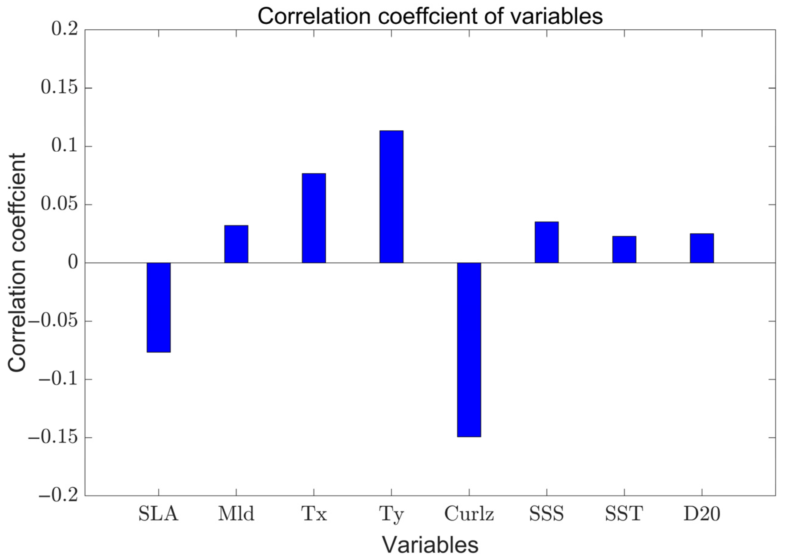
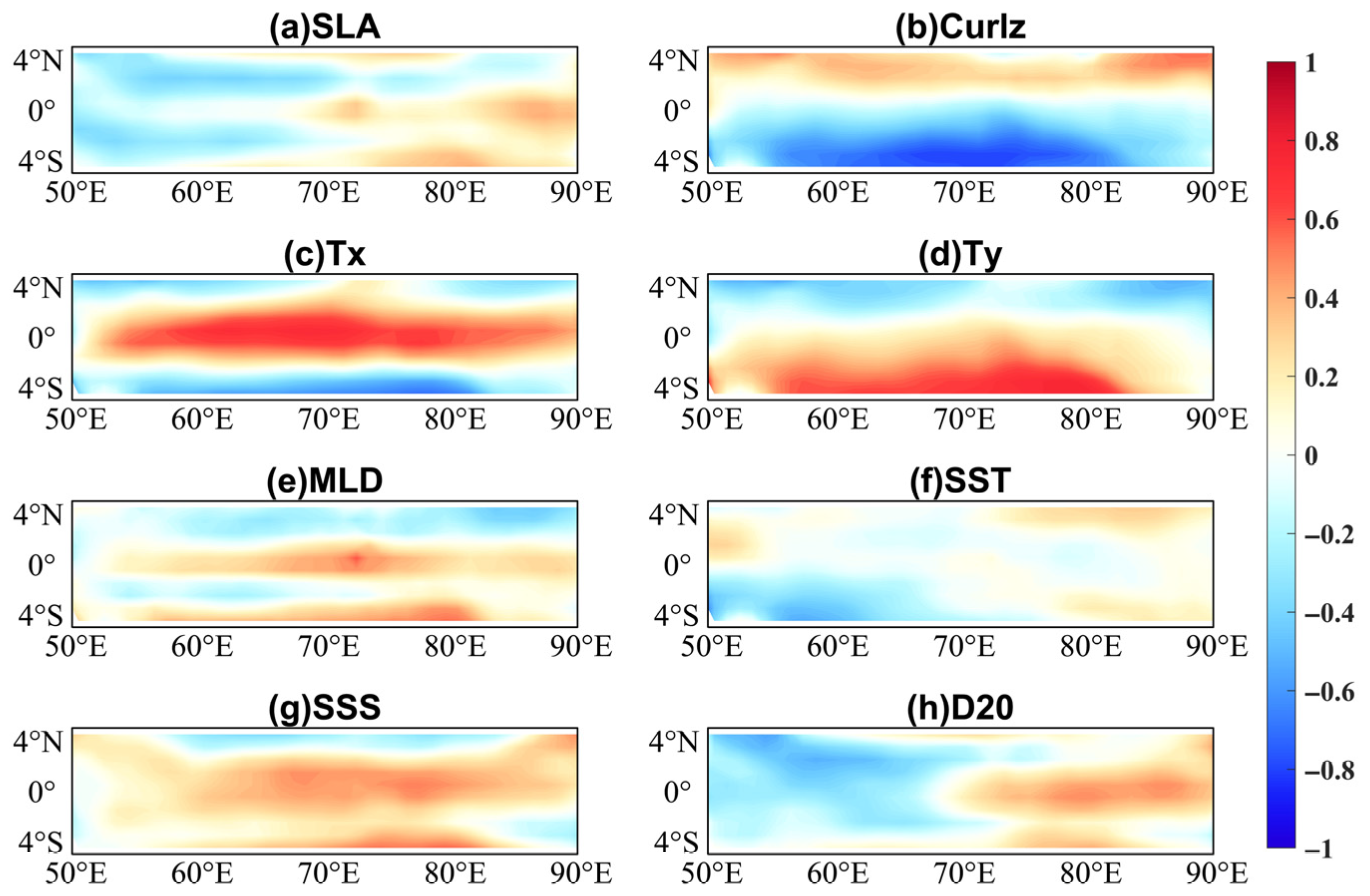
3.1. Correlation Analysis Between U and Sea Surface Parameters

Figure 2 illustrates the monthly satellite-derived sea surface parameters over the equatorial Indian Ocean in February (a1–h1), May (b2–h2), August (c3–h3), and November (d4–h4) of 2022. The parameters included MLD, Curlz, Tx, Ty, SLA, SST, SSS, and D20. Across the entire equatorial region, each parameter exhibits pronounced spatial patterns and heterogeneous characteristics, which vary significantly with seasonal changes.
In winter (February), The MLD is shallower near the equator (Figure 2(a1)). The Curlz displays a relatively uniform spatial distribution (Figure 2(b1)). The Tx is predominantly eastward, driven by persistent westerlies associated with the Northeast Monsoon (Figure 2(c1)). The southward Ty is relatively strong during the Northeast Monsoon (Figure 2(d1)). SLA is generally low, indicating a relatively stable ocean state (Figure 2(e1)). SST is higher in the equatorial region (Figure 2(f1)), while SSS is more uniformly distributed, with slightly higher salinity near the equator (Figure 2(g1)). D20 is uniformly distributed in the equatorial region, with an east–west difference of less than 20 m (Figure 2(h1)).
In spring (May), the MLD deepens in the eastern region (70° E–90° E) (Figure 2(a2)), corresponding to enhanced zonal wind stress (Tx > 0.02 N/m2) during the early southwest monsoon (Figure 2(c2)). The negative regions of Curlz expand eastward toward the equator, with locally enhanced negative curl in the western Indian Ocean (50° E–70° E) (Figure 2(b2)). The Ty shifts to a northward direction, accompanied by a reversal of cross-equatorial airflow (Figure 2(d2)). SLA rises in the eastern equatorial region due to enhanced westerly wind (Figure 2(e2)). SST exhibits significant warming (29–30 °C) in the region of 50° E–75° E (Figure 2(f2)). The decreases to approximately 35 PSU in the eastern equatorial region, while it remains relatively high in the western equatorial region (Figure 2(g2)). The depth of D20 reaches the maximum of −120 m, accompanied with westerly wind (Figure 2(h2)).
In summer (August), the MLD is about 40 m in the central equatorial region, with a slightly deeper mixed layer on the western and eastern equatorial region (Figure 2(a3)). A pronounced negative Curlz region is observed, particularly on the western equatorial region (Figure 2(b3)). The wind stress directions of Tx are opposite north and south of the equator, with positive values in north of the equator and negative values south of the equator (Figure 2(c3)). A positive Ty significantly strengthens west of 70° E (Figure 2(d3)). SLA on the western side of the equator reaches the maximum (Figure 2(e3)). SST shows significant cooling in the western equatorial region, while the high SST expands on the eastern side (Figure 2(f3)). SSS decreases along the equator (Figure 2(g3)). D20 reaches its maximum in the western equatorial region (Figure 2(h3)).
In autumn (November), MLD generally shoals and reaches the minimum in the western equatorial region (Figure 2(a4)). Curlz is positive north of the equator but negative south of equator (Figure 2(b4)). A positive Tx dominates the equator region (Figure 2(c4)), while Ty is relatively weak in the equator region (Figure 2(d4)). SLA strengthens on the eastern side, accompanied by westerly wind (Figure 2(e4)). SST is relatively uniform in the equatorial region (Figure 2(f4)). SSS reaches the maximum in the region of 60° E–70° E, 0–4° N (Figure 2(g4)). D20 deepens in the eastern equatorial region, accompanied by westerly wind (Figure 2(h4)).
Figure 3 illustrates the spatial correlations between various parameters and zonal velocity (U) from OSCAR data during 1993–2022. In the equatorial region, wind stress parameters exhibit the most pronounced influence on U. Specifically, Tx demonstrates a high positive correlation with U, reaching a correlation coefficient of 0.8 (Figure 3c). Ty also shows a positive correlation with U, with a correlation coefficient of 0.6 south of the equator, albeit slightly lower than that of Tx (Figure 3d). Curlz demonstrates a low positive correlation with U north of the equator and a high negative correlation with U south of the equator (Figure 3b). Both MLD (Figure 3d) and SSS (Figure 3g) display moderate positive correlations with U, and their correlation coefficients are less than 0.5. Both SLA (Figure 3a) and D20 (Figure 3h) demonstrate low negative correlations with U west of 70° E and positive correlations with U east of 70° E, with their correlation coefficients less than 0.2. In contrast, SST exhibits weak negative correlations with U in the equatorial region, with correlation coefficients less than −0.2 (Figure 3f), suggesting their relatively limited influence on WJ dynamics.

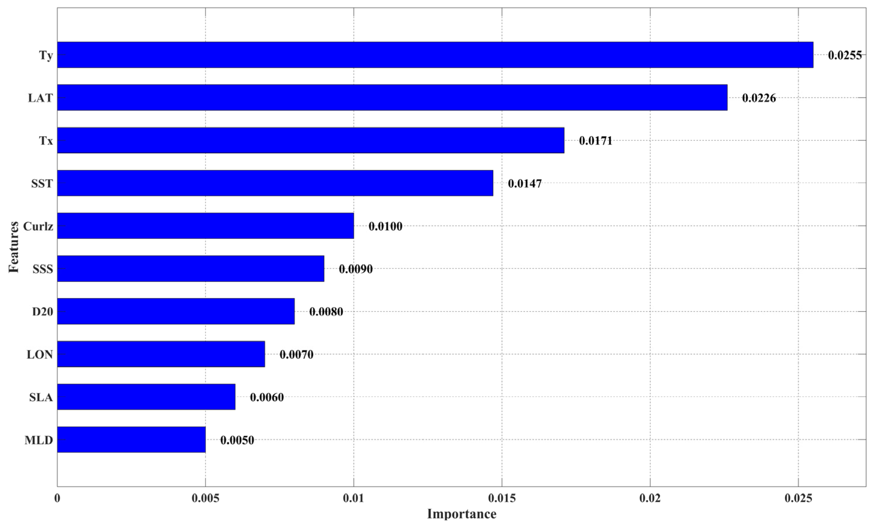
3.2. Identification of Input Variables

Table 2 demonstrates the feature importance distributions across different models for each case, where each row corresponds to an individual case and each column represents a feature parameter. In this study, we progressively increased the number of input parameters to evaluate their impact on model performance: Case 1 exclusively utilized two sea surface parameters (Tx and Ty) as input variables; Case 2 expanded to three sea surface parameters (Tx, Ty, and SSS); this progression continued until Case 9 incorporated all 10 parameters. By sequentially inputting each case into the models, we systematically assessed the influence of diverse parameter combinations on the model inversion capability, ultimately identifying the optimal parameter set. Figure 4 further compares the model performance metrics across cases, providing a quantitative basis for parameter selection.
To precisely evaluate and select parameters as input variables, this study adopted RMSE, MAE, and R2 as key evaluation metrics. Comparative analysis of model performance enables clear identification of performance disparities across cases in these metrics. As illustrated in Figure 4, Case 1 exhibited the highest MAE (0.14 m/s) and RMSE (0.18 m/s) values among all configurations, accompanied by the lowest R2 (0.55), indicating its maximum inversion error and weakest correlation. In contrast, Case 9 demonstrated superior performance with the lowest MAE (0.06 m/s), minimal RMSE (0.08 m/s), and optimal R2 (0.9), signifying the highest reconstruction accuracy. Based on this comprehensive analysis, Case 9 was selected as the optimal model configuration, with its parameter set established as the definitive input variables for the model.

3.3. Evaluation of the XGBoost Model

In order to comprehensively evaluate the performance of the XGBoost model in reconstructing the seasonal variability of the WJ, we developed the XGBoost framework to estimate the zonal velocity of the WJ in the equatorial Indian Ocean. Figure 5 presents the horizontal distributions of the WJ derived from OSCAR data during spring (Figure 5a), summer (Figure 5c), autumn (Figure 5e), and winter (Figure 5g) of 2022. Notably, the WJ peaks in autumn (approximately 0.6 m/s), significantly exceeding spring velocity (−0.3 m/s), demonstrating pronounced seasonal disparities. These results align with previous studies [1,7,8], further corroborating the seasonal variability of WJ in this region.
The spatial distributions of WJ velocity estimated by the XGBoost model (Figure 5b,d,f,h) exhibited superior consistency with the zonal velocity distributions from OSCAR data (Figure 5a,c,e,g), confirming the model’s capability of accurately reconstructing both the spatial patterns and seasonal dynamics of the WJ. Therefore, the XGBoost model could be used for seasonal variability reconstruction of the WJ.
To comprehensively evaluate the performance of the XGBoost model in reconstructing the WJ, we analyzed the spatial distributions of discrepancies between the WJ velocity derived from both machine learning models and those from the OSCAR dataset (Figure 6). The results demonstrated that the differences between XGBoost-reconstructed and OSCAR-based WJ velocity were generally smaller, particularly during spring (Figure 6a) and autumn (Figure 6c), in which errors remained below 0.05 m/s. Although slightly higher discrepancies were observed in summer (Figure 6b) and winter (Figure 6d), the overall errors were still constrained to less than 0.1 m/s. Consequently, the XGBoost model demonstrated superior performance in reconstructing the Wyrtki Jet in the equatorial Indian Ocean, establishing its efficacy for reconstructing regional oceanic circulation dynamics.
To further investigate the reconstruction performance of the XGBoost model for the Wyrtki Jet within the study region (50° E–90° E, 5° S–5° N), Figure 7 presents seasonal scatterplots comparing the XGBoost-reconstructed jet velocity with the corresponding OSCAR dataset during spring (Figure 7a), summer (Figure 7b), autumn (Figure 7c), and winter (Figure 7d). The data points were mainly concentrated near the contour lines, indicating strong agreement between model reconstructions and observational data. To quantify this consistency, R2 and RMSE were employed as the evaluation metrics. The results demonstrated that the XGBoost-reconstructed WJ velocity exhibited strong agreement with OSCAR-derived data across all seasons, achieving consistent R2 values of 0.97 and RMSE ≤ 0.2 and confirming the model’s robust capability to capture seasonal variations. This robust performance highlights the effectiveness and reliability of the XGBoost model in reconstructing oceanic zonal current dynamics, solidifying its utility for high precision marine current reconstruction in the equatorial Indian Ocean.
To thoroughly evaluate the performance of the XGBoost model in reconstructing seasonal variations of the WJ zonal velocity in the equatorial Indian Ocean, the spatial distribution of WJ zonal velocity from OSCAR and XGBoost model in 2022 is shown in Figure 8. The observational results revealed pronounced seasonal variability in WJ zonal velocity: the velocity peaks at approximately 0.6 m/s in November (Figure 8g), corresponding to the intensified phase of the autumn WJ, while the May peak (Figure 8c) reaches approximately 0.4 m/s, aligning with the active period of the spring WJ. Additionally, the WJ exhibited stable westward flow in February (Figure 8a) and weaker eastward flow in August (Figure 8e), which is closely linked to the seasonal transition of the Indian Ocean monsoon. In model performance comparisons, the XGBoost-reconstructed spatial distributions of WJ zonal velocity (Figure 8b,d,f,h) showed high consistency with OSCAR observations (Figure 8a,c,e,g), particularly in Feburary, May, August, and November. The XGBoost model effectively captured both the high-velocity core regions and spatial extents of WJ.
To further quantify the discrepancies between model reconstructions and observational data, Figure 9 presents the error distributions of the XGBoost-reconstructed WJ zonal velocity relative to the OSCAR dataset. The results demonstrated that the XGBoost-reconstructed velocity exhibited relatively smaller errors (Figure 9a–d), In February, May, and November, regions with an error of 0.2 m/s were mainly in 50° E–60° E, and other regions had an error of about 0.05 m/s. In August, the regions with an error of 0.2 m/s shifted to 60° E–70° E, and other regions still had a low error of about 0.05 m/s. Comprehensive analysis revealed that both models effectively captured the temporal variability of WJ zonal velocity, and the XGBoost model demonstrated superior overall accuracy and stability, consistently maintaining lower reconstruction errors across all months.
To quantitatively assess the XGBoost model’s reconstruction of the WJ zonal velocity, scatter plots comparing the model output with OSCAR observational data are presented for February (Figure 10a), May (Figure 10b), August (Figure 10c), and November (Figure 10d). Evaluation using R2 and RMSE metrics revealed significant seasonal variations in reconstruction accuracy. The model demonstrated optimal performance in February (Figure 10a; R2 = 0.97, RMSE = 0.03 m/s), precisely capturing the WJ velocity dynamics. High performance was also evident in May (Figure 10b; R2 = 0.96, RMSE = 0.04 m/s) and November (Figure 10d; R2 = 0.95, RMSE = 0.05 m/s). While August (Figure 10c) showed a moderate reduction in correlation (R2 = 0.90, RMSE = 0.07 m/s), performance remained statistically robust. Following the July peak, the WJ started to weaken rapidly and nearly vanished. These results confirmed the high reliability of the XGBoost model in reconstructing WJ zonal velocity and its capacity to characterize seasonal variability within the study domain, underscoring its substantial applicability for simulating WJ dynamics in the equatorial Indian Ocean.
Figure 11 illustrates the seasonal variability of the WJ zonal velocity within the study region (50° E–80° E, 3° S–3° N) during 2022, comparing observational data from the OSCAR dataset with reconstruction results obtained from the XGBoost model. The OSCAR observations demonstrated distinct seasonal dynamics, with the WJ zonal velocity peaking at 0.35 m/s in November, followed by 0.31 m/s in May. A notable decline was observed in August (0.11 m/s), reaching the minimum of −0.20 m/s in February. These variations are closely associated with the semi-annual reversals of the Indian Ocean monsoon system.
The reconstruction results of the XGBoost model demonstrated exceptional consistency with observational data, successfully capturing the seasonal extremes of zonal velocity in the WJ in the equatorial Indian Ocean: the minimum value (−0.21 m/s) in February and the maximum value (0.35 m/s) in November. The reconstructions exhibited near-perfect correlation with the OSCAR data (R2 = 0.99) and an ultra-low root mean square error (RMSE = 0.004 m/s), robustly validating the model’s reliability in resolving the seasonal variability of the WJ. A marginal underestimation (0.01 m/s error) was observed in September but remained within acceptable thresholds.

4. Discussion

Figure 12 presents a comparison between the XGBoost-reconstrusted and OSCAR zonal velocities of the WJ in the study region of 50° E–80° E, 3° S–3° N in 2013, illustrating distinct seasonal patterns. OSCAR data showed the WJ reaching a peak of 0.32 m/s in May, with velocities at −0.15 m/s in April and November, a velocity of 0.03 m/s in August, and a low velocity of −0.16 m/s in February. This indicates the WJ’s asymmetric seasonal pattern in 2013, with higher velocities in spring (May) compared to autumn (November). The XGBoost results aligned closely with OSCAR, capturing the minimum (−0.14 m/s) in February and maximum (0.30 m/s) in May with a high R2 of 0.99 and a low RMSE of 0.01 m/s. However, a slight underestimation (0.01 m/s error) occurred in December but was within the acceptable error range. The model successfully captured the opposite WJ seasonal modes in 2013 and 2022, confirming the XGBoost’s robustness in WJ seasonal reconstruction.
Combing the daily RAMA observation data, we can extend the XGBoost to long-term sequence reconstruction of the Wyrtki Jet (WJ) at daily intervals, further examining its sub-seasonal to interannual variability characteristics. Additionally, the XGBoost framework demonstrates exceptional efficiency and precision in processing large-scale datasets, with intrinsic regularization mechanisms effectively mitigating overfitting, thereby exhibiting significant potential for subsurface current velocity prediction. In the future, we will deploy the XGBoost model for seasonal reconstruction of the Equatorial Undercurrent (EUC). Nevertheless, we explicitly recognize the inherent limitations in modeling highly complex nonlinear relationships, manifesting as risks of underfitting or overfitting. To address these challenges, we outline three strategic enhancements: primary implementation of advanced feature engineering to comprehensively extract informational patterns; secondary integration of transformer architectures, leveraging their superior sequential modeling capabilities to elevate reconstruction accuracy; and tertiary incorporation of physical oceanographic knowledge through domain-specific constraints to augment model interpretability and predictive fidelity. Collectively, these methodological refinements will enable more precise reconstruction of subsurface equatorial currents, ultimately delivering innovative solutions for marine hazard mitigation, mariculture operations, and environmental conservation initiatives.

5. Conclusions

This study investigated the seasonal variability of the WJ in the equatorial Indian Ocean using satellite observations and machine learning models (XGBoost). The results demonstrated that wind stress components (Tx and Ty), SST, and wind stress curl were the dominant factors influencing the seasonal variability of the WJ. The XGBoost model outperformed LightGBM in reconstructing the WJ and its seasonal variations, achieving R2 values exceeding 0.97 across all seasons and maintaining root mean square errors (RMSE) below 0.2 m/s across all seasons. The discrepancies between the XGBoost-reconstructed zonal velocity and the OSCAR dataset were notably small, with errors below 0.05 m/s in summer and winter and below 0.1 m/s in spring and autumn, confirming its robustness and reliability.
The study also revealed significant seasonal variations in the velocity of the Wyrtki Jet in the equatorial Indian Ocean: the maximum velocity occurs in autumn (approximately 0.5 m/s), followed by spring (around 0.3 m/s), with summer velocities averaging 0.11 m/s and winter reaching the minimum (about −0.21 m/s). The XGBoost model demonstrated a significantly positive correlation between its estimated Wyrtki Jet velocities and the zonal velocity (U) derived from OSCAR data, validating its accuracy and reliability in capturing the seasonal variations of the jet’s zonal flow. These results highlight the superior performance of the XGBoost model in zonal velocity inversion for the equatorial Indian Ocean Wyrtki Jet, providing precise data support for research on regional ocean circulation dynamics and effectively addressing the observational gaps in current velocity measurements for this critical current system.
The XGBoost model stands out for its streamlined architecture, which directly integrates multiple parameters to accurately extract feature information from variables and comprehensively account for their interactions. However, as a data-driven model, it exhibits inherent limitations, such as tendencies toward overestimation or underestimation. Notably, the zonal velocity of the Wyrtki Jet is also influenced by ocean dynamic and thermodynamic processes. Future research will incorporate additional marine dynamic mechanisms to enhance the estimation precision of Wyrtki Jet zonal flow velocities. The multi-source feature fusion modeling framework proposed in this study provides a high spatial temporal-resolution tool for investigating tropical Indian Ocean circulation dynamics, offering critical data support for analyzing monsoon–ocean current coupling mechanisms, early warning of extreme climate events, and regional resource management.

Author Contributions

D.L.: data analysis; writing—original draft; S.Z.: study design; writing—review and editing. C.Z.: concepts discussed; writing—review and editing; L.X. and L.Y.: concepts discussed; suggestions provided. All authors have read and agreed to the published version of the manuscript.

Funding

This study was supported by the Innovative Team Plan for Department of Education of Guangdong Province (2023KCXTD015), the First-class Discipline Plan of Guangdong Province (080508032401, 010202032401), and the program for scientific research start-up funds of Guangdong Ocean University (R19061, 060302032104).

Data Availability Statement

The datasets presented in this study are publicly available.

Acknowledgments

The monthly wind data were obtained from https://cds.climate.copernicus.eu/cdsapp#!/dataset/reanalysis-era5-single-levels-monthly-means?tab=overview (accessed on 10 June 2023). The SLA data were obtained from http://www.aviso.altimetry.fr/en/home.html (accessed on 9 June 2023). The OSCAR U data were obtained from https://www.esr.org/research/oscar/ (accessed on 10 June 2023). D20, SSS, SST, and MLD were obtained from https://cds.climate.copernicus.eu/datasets/reanalysis-oras5?tab=download (accessed on 8 June 2023). RAMA U data were obtained from https://www.pmel.noaa.gov/tao/drupal/disdel/ (accessed on 7 June 2023).

Conflicts of Interest

The authors declare no conflicts of interest.

Appendix A

Appendix A.1. Validation of OSCAR Reanalysis Data Against RAMA Mooring Observations

To validate the accuracy of OSCAR reanalysis data in the equatorial Indian Ocean, this study systematically evaluated the dataset using in situ velocity measurements. Daily velocity observations from the Research Moored Array for African-Asian-Australian Monsoon Analysis and Prediction (RAMA) were employed to assess OSCAR velocity products in the same region. Raw RAMA data underwent 5-day averaging to match the temporal resolution of the reanalysis dataset. As shown in Figure A1, six representative stations were selected for validation: 67° E, 0° N (Figure A1a), 80.5° E, 0° N (Figure A1b), 90° E, 0° N (Figure A1c), 67° E, 1.5° N (Figure A1d), 67° E, 1.5° S (Figure A1e) and 67° E, 4° N (Figure A1f). Comparison of the zonal velocity time series at 10 m depth demonstrated that OSCAR reanalysis data accurately captured temporal variation characteristics of measured velocities across three representative stations. This confirms its ability to reliably characterize near-surface current dynamics in the equatorial Indian Ocean. Based on this validation, OSCAR data were subsequently used for seasonal-scale reconstruction of the Wyrtki Jet (WJ) in this study.
Figure A1. Comparison of the zonal current velocity time series at 10 m depth between OSCAR reanalysis data (red line) and RAMA observed data (blue line): (a) 67° E, 0° N; (b) 80.5° E, 0° N; (c) 90° E, 0° N, (d) 67° E, 1.5° N; (e) 67° E, 1.5° S; (f) 67° E, 4° N.
Algorithms 18 00431 g0a1

Appendix A.2. XGBoost-Based Reconstruction Framework for Wyrtki Jet Zonal Currents

During the development of machine learning models, datasets are typically divided into three independent subsets: training data, validation data, and test data. The training data are used to optimize model parameters, while the validation data evaluate model performance during training, guide hyperparameter tuning, and control overfitting risks. The test data, functioning as an independent evaluation set, are primarily utilized for an unbiased assessment of the generalization capability of the model on unseen data, thereby rigorously validating the reliability of the model in practical applications. In this study, all data from January 1993 to December 2022 were randomly divided into three parts: training, validation, and test sets. We used 348 months of data for training, with 80% randomly selected for training and 20% for validation. An additional 12 months of data were used for testing to evaluate the final model performance. The proposed XGBoost model flowchart is shown in Figure A2. The application process involves two main steps: (1) model training and validation; and (2) using the trained model to estimate WJ zonal current speed. Prior to applying the models to reconstruct the WJ zonal current, we trained and validated it using satellite sea surface data and OSCAR labeled data. Based on prior research, we selected SLA, Tx, Ty, Curlz, MLD, D20, SSS, SST, and geographical information (longitude and latitude) as independent input variables for the machine learning model to estimate the zonal speed of the WJ in the equatorial Indian Ocean. Furthermore, we used a separate XGBoost model to estimate WJ zonal speed based on sea surface data.
Figure A2. Flowchart of the XGBoost model for estimating the zonal velocity of the Wyrtki Jet in the equatorial Indian Ocean.
Algorithms 18 00431 g0a2

Appendix A.3. Correlation Analysis of Marine Parameters with U

Based on the spatial correlation analysis between various marine parameters and U during 1993–2022, the primary dynamical factors influencing the interannual variability of U were revealed. To further explore the transient response characteristics of environmental factors on the equatorial zonal velocity at the seasonal scale, Figure A3 focuses on the year 2022 and provides in-depth insights by analyzing the correlation coefficients between each parameter and the WJ. Figure A3 displays the correlation coefficients between U from the OSCAR dataset and various parameters in 2022, including SLA, MLD, Tx, Ty, CurlZ, SSS, SST, and D20. The results indicate that Ty and Tx exhibited significant positive correlations with U, with correlation coefficients of 0.11 and 0.07, respectively. This suggests that wind stress is a key dynamic factor influencing zonal velocity in the equatorial region. The increase in wind stress, closely related to monsoon activity and seasonal changes in atmospheric circulation, can directly accelerate the zonal movement of surface seawater. Additionally, SSS and MLD showed relatively strong positive correlations with U, with correlation coefficients of 0.04 and 0.03. This implies that SSS and MLD may indirectly regulate surface current intensity by affecting oceanic density stratification and vertical mixing processes. In contrast, SST and D20 had weak correlations with U, with correlation coefficients of 0.022 and 0.025, indicating limited direct thermal control over zonal velocity in 2022. Notably, SLA and Curlz showed negative correlations with U, with correlation coefficients of −0.08 and −0.15. The negative correlation of SLA may be linked to geostrophic flow effects, in which elevated sea levels correspond to weakened eastward flow. The negative correlation of Curlz was associated with wind-driven Ekman upwelling; an increase in wind stress curl strengthens upwelling, which suppresses the acceleration of zonal velocity.
Figure A3. Correlation coefficients between the zonal velocity of the Wyrtki Jet from the OSCAR dataset and various input parameters in 2022.
Algorithms 18 00431 g0a3

Appendix A.4. Feature Importance Analysis of Marine Parameters in WJ Reconstruction

In the reconstruction of the WJ in the equatorial Indian Ocean, marine environmental parameters differed in their contributions to model accuracy. To explore the importance weights of various input factors in model training and enhance the regression fitting process to approach the OSCAR-observed current values (U) for optimal inversion accuracy, this study used the XGBoost machine learning model to calculate the importance scores of 10 marine environmental parameters for U reconstruction, with 4 significant digits retained. The higher the importance score, the greater the parameter’s contribution to the reconstruction results. Figure A4 shows the feature importance analysis results of the XGBoost model. The top five parameters and their scores were Ty (0.0255), LAT (0.0226), Tx (0.0171), SST (0.0147), and Curlz (0.0100). Ty reflects the north and south movement of the WJ axis, while Tx mainly influence the eastward current movement and related wind stress curl changes, which often lead to temperature increases in the eastern equatorial Indian Ocean.
The other parameters, namely SSS, D20, LON, SLA, and MLD, had smaller contributions, with importance scores of 0.009, 0.008, 0.007, 0.006, and 0.005. Notably, the eastward WJ movement drove dynamical response in the eastern equatorial Indian Ocean, which manifested as increased salinity, a deepening of D20, elevated SLA, and a thickening of MLD. These results revealed the distinct roles of marine environmental parameters in U inversion, offering a basis for model optimization and key parameter selection in future studies.
Figure A4. Feature importance of input parameters for the XGBoost model.
Algorithms 18 00431 g0a4

References

  1. Wyrtki, K. An Equatorial Jet in the Indian Ocean. Science 1973, 181, 262–264. [Google Scholar] [CrossRef] [PubMed]
  2. Haiming, X. Seasonal variability of the west-east water mass exchange on the section of central equatorial Indian Ocean and its regional difference. Acta Oceanol. Sin. 2012, 30, 1082–1092. [Google Scholar] [CrossRef]
  3. Sun, Q.; Zhang, Y.; Du, Y.; Jiang, X. Asymmetric Response of Sea Surface Salinity to Extreme Positive and Negative Indian Ocean Dipole in the Southern Tropical Indian Ocean. J. Geophys. Res.-Ocean. 2022, 127, e2022JC018986. [Google Scholar] [CrossRef]
  4. Murtugudde, R.; Busalacchi, A.J. Interannual Variability of the Dynamics and Thermodynamics of the Tropical Indian Ocean. J. Clim. 1999, 12, 2300–2326. [Google Scholar] [CrossRef]
  5. Vinayachandran, P.N.; Saji, N.H.; Yamagata, T. Response of the equatorial Indian Ocean to an unusual wind event during 1994. Geophys. Res. Lett. 1999, 26, 1613–1616. [Google Scholar] [CrossRef]
  6. Chatterjee, A.; Shankar, D.; McCreary, J.P.; Vinayachandran, P.N.; Mukherjee, A. Dynamics of Andaman Sea circulation and its role in connecting the equatorial Indian Ocean to the Bay of Bengal. J. Geophys. Res. Ocean. 2017, 122, 3200–3218. [Google Scholar] [CrossRef]
  7. Molinari, R.L.; Olson, D.; Reverdin, G. Surface current distributions in the tropical Indian Ocean derived from compilations of surface buoy trajectories. J. Geophys. Res. Ocean. 1990, 95, 7217–7238. [Google Scholar] [CrossRef]
  8. Qiu, Y.; Li, L.; Yu, W. Behavior of the Wyrtki Jet observed with surface drifting buoys and satellite altimeter. Geophys. Res. Lett. 2009, 36, 120–131. [Google Scholar] [CrossRef]
  9. Duan, Y.; Liu, L.; Han, G.; Liu, H.; Yu, W.; Yang, G.; Wang, H.; Wang, H.; Liu, Y.; Zahid; et al. Anomalous behaviors of Wyrtki Jets in the equatorial Indian Ocean during 2013. Sci. Rep. 2016, 6, 29688. [Google Scholar] [CrossRef]
  10. Joseph, S.; Wallcraft, A.J.; Jensen, T.G.; Ravichandran, M.; Shenoi, S.S.C.; Nayak, S. Weakening of spring Wyrtki jets in the Indian Ocean during 2006–2011. J. Geophys. Res.-Ocean. 2012, 117, C04012. [Google Scholar] [CrossRef]
  11. Reppin, J.R.; Schott, F.A.; Fischer, J.; Quadfasel, D. Equatorial currents and transports in the upper central Indian Ocean: Annual cycle and interannual variability. J. Geophys. Res.-Ocean. 1999, 104, 15495–15514. [Google Scholar] [CrossRef]
  12. Chen, G.; Han, W.; Li, Y.; Wang, D.; McPhaden, M.J. Seasonal-to-Interannual Time-Scale Dynamics of the Equatorial Undercurrent in the Indian Ocean. J. Phys. Oceanogr. 2015, 45, 1532–1553. [Google Scholar] [CrossRef]
  13. Deng, K.; Cheng, X.; Feng, T.; Ma, T.; Duan, W.; Chen, J. Interannual variability of the spring Wyrtki Jet. J. Oceanol. Limnol. 2021, 39, 26–44. [Google Scholar] [CrossRef]
  14. Schott, F.A.; McCreary, J.P. The monsoon circulation of the Indian Ocean. Prog. Oceanogr. 2001, 51, 1–123. [Google Scholar] [CrossRef]
  15. Rao, R.R.; Molinari, R.L.; Festa, J.F. Evolution of the climatological near-surface thermal structure of the tropical Indian Ocean: 1. Description of mean monthly mixed layer depth, and sea surface temperature, surface current, and surface meteorological fields. J. Geophys. Res. Ocean. 1989, 94, 10801–10815. [Google Scholar] [CrossRef]
  16. Masumoto, Y.; Hase, H.; Kuroda, Y.; Matsuura, H.; Takeuchi, K. Intraseasonal variability in the upper layer currents observed in the eastern equatorial Indian Ocean. Geophys. Res. Lett. 2005, 32, L02607. [Google Scholar] [CrossRef]
  17. McPhaden, M.J.; Meyers, G.; Ando, K.; Masumoto, Y.; Murty, V.S.N.; Ravichandran, M.; Syamsudin, F.; Vialard, J.; Yu, L.; Yu, W. RAMA: The Research Moored Array for African–Asian–Australian Monsoon Analysis and Prediction. Bull. Am. Meteorol. Soc. 2009, 90, 459–480. [Google Scholar] [CrossRef]
  18. Zhang, J.; Liu, B.; Ren, S.; Han, W.; Ding, Y.; Peng, S. A 4 km daily gridded meteorological dataset for China from 2000 to 2020. Sci. Data 2024, 11, 1230. [Google Scholar] [CrossRef]
  19. Mak, H.W.L.; Laughner, J.L.; Fung, J.C.H.; Zhu, Q.; Cohen, R.C. Improved Satellite Retrieval of Tropospheric NO2 Column Density via Updating of Air Mass Factor (AMF): Case Study of Southern China. Remote Sens. 2018, 10, 1789. [Google Scholar] [CrossRef]
  20. Noone, S.; Atkinson, C.; Berry, D.I.; Dunn, R.J.H.; Freeman, E.; Perez Gonzalez, I.; Kennedy, J.J.; Kent, E.C.; Kettle, A.; McNeill, S.; et al. Progress towards a holistic land and marine surface meteorological database and a call for additional contributions. Geosci. Data J. 2021, 8, 103–120. [Google Scholar] [CrossRef]
  21. Perez, J.d.J.S.; Garza, A.G.J.; Monreal, D.S. Dataset on meteorological forcing mechanisms impacting marine circulation and oceanographic variables in the northern part of the Veracruz reef system. Data Brief 2023, 51, 109637. [Google Scholar] [CrossRef] [PubMed]
  22. Wu, L.C.; Doong, D.J.; Lai, J.W. Sea Surface Current Estimation from a Semi-Enclosed Bay Using Coastal X-Band Radar Images. IEEE Trans. Geosci. Remote Sens. 2024, 62, 1–11. [Google Scholar] [CrossRef]
  23. Zhu, Z.; Geng, X.; Li, S.; Xie, T.; Yan, X.-H. Ocean surface current retrieval at Hangzhou Bay from Himawari-8 sequential satellite images. Sci. China Earth Sci. 2020, 63, 1026–1038. [Google Scholar] [CrossRef]
  24. Fablet, R.; Febvre, Q.; Chapron, B. Multimodal 4DVarNets for the Reconstruction of Sea Surface Dynamics From SST-SSH Synergies. IEEE Trans. Geosci. Remote Sens. 2023, 61, 1–14. [Google Scholar] [CrossRef]
  25. Yang, X.; Chong, J.; Zhao, Y. Sea Surface Current Retrieval From Sequential SAR and Ocean Color Images for Eddy Kinematics Analysis: A Case Study in the Northern Tyrrhenian Sea. IEEE J. Sel. Top. Appl. Earth Obs. Remote Sens. 2024, 17, 10126–10136. [Google Scholar] [CrossRef]
  26. Sun, W.; Jia, C.; Fan, C.; Li, W.; Dai, Y.; Huang, W. Maximum a Posteriori Based Ocean Surface Current Inversion for Doppler Scatterometer. IEEE J. Sel. Top. Appl. Earth Obs. Remote Sens. 2024, 17, 2067–2076. [Google Scholar] [CrossRef]
  27. Sun, J.; Li, H.; Lin, W.; He, Y. Joint Inversion of Sea Surface Wind and Current Velocity Based on Sentinel-1 Synthetic Aperture Radar Observations. J. Mar. Sci. Eng. 2024, 12, 450. [Google Scholar] [CrossRef]
  28. Ciani, D.; Rio, M.-H.; Menna, M.; Santoleri, R. A Synergetic Approach for the Space-Based Sea Surface Currents Retrieval in the Mediterranean Sea. Remote Sens. 2019, 11, 1285. [Google Scholar] [CrossRef]
  29. Bao, Q.; Lin, M.; Zhang, Y.; Dong, X.; Lang, S.; Gong, P. Ocean Surface Current Inversion Method for a Doppler Scatterometer. IEEE Trans. Geosci. Remote Sens. 2017, 55, 6505–6516. [Google Scholar] [CrossRef]
  30. Wang, W.; Zhou, H.; Zheng, S.; Lü, G.; Zhou, L. Ocean surface currents estimated from satellite remote sensing data based on a global hexagonal grid. Int. J. Digit. Earth 2023, 16, 1073–1093. [Google Scholar] [CrossRef]
  31. Su, H.; Wu, X.; Yan, X.-H.; Kidwell, A. Estimation of subsurface temperature anomaly in the Indian Ocean during recent global surface warming hiatus from satellite measurements: A support vector machine approach. Remote Sens. Environ. 2015, 160, 63–71. [Google Scholar] [CrossRef]
  32. Su, H.; Huang, L.; Li, W.; Yang, X.; Yan, X.H. Retrieving Ocean Subsurface Temperature Using a Satellite-Based Geographically Weighted Regression Model. J. Geophys. Res. Ocean. 2018, 123, 5180–5193. [Google Scholar] [CrossRef]
  33. Zhang, S.Y.; Yang, Y.Z.; Xie, K.W.; Gao, J.H.; Zhang, Z.Y.; Niu, Q.R.; Wang, G.J.; Che, Z.H.; Mu, L.; Jia, S. Spatial-Temporal Siamese Convolutional Neural Network for Subsurface Temperature Reconstruction. IEEE Trans. Geosci. Remote Sens. 2024, 62, 1–16. [Google Scholar] [CrossRef]
  34. Leupold, M.; Pfeiffer, M.; Watanabe, T.K.; Reuning, L.; Garbe-Schönberg, D.; Shen, C.C.; Brummer, G.J.A. El Nino-Southern Oscillation and internal sea surface temperature variability in the tropical Indian Ocean since 1675. Clim. Past 2021, 17, 151–170. [Google Scholar] [CrossRef]
  35. Nairn, M.G.; Lear, C.H.; Sosdian, S.M.; Bailey, T.R.; Beavington-Penney, S. Tropical Sea Surface Temperatures Following the Middle Miocene Climate Transition From Laser-Ablation ICP-MS Analysis of Glassy Foraminifera. Paleoceanogr. Paleoclimatol. 2021, 36, e2020PA004165. [Google Scholar] [CrossRef]
  36. Burdanowitz, N.; Rixen, T.; Gaye, B.; Emeis, K.C. Signals of Holocene climate transition amplified by anthropogenic land-use changes in the westerly-Indian monsoon realm. Clim. Past 2021, 17, 1735–1749. [Google Scholar] [CrossRef]
  37. Ding, X.; Bassinot, F.; Pang, X.L.; Kou, Y.X.; Zhou, L.P. Heat Transport Processes of the Indonesian Throughflow Along the Outflow Pathway in the Eastern Indian Ocean During the Last 160 Kyr. Paleoceanogr. Paleoclimatol. 2023, 38, e2023PA004620. [Google Scholar] [CrossRef]
  38. Shi, X.F.; Liu, S.F.; Zhang, X.; Sun, Y.C.; Cao, P.; Zhang, H.; Li, X.Y.; Xu, S.; Qiao, S.Q.; Khokiattiwong, S.; et al. Millennial-scale hydroclimate changes in Indian monsoon realm during the last deglaciation. Quat. Sci. Rev. 2022, 292, 107702. [Google Scholar] [CrossRef]
  39. Tiger, B.H.; Burns, S.; Dawson, R.R.; Scroxton, N.; Godfrey, L.R.; Ranivoharimanana, L.; Faina, P.; McGee, D. Zonal Indian Ocean Variability Drives Millennial-Scale Precipitation Changes in Northern Madagascar. Paleoceanogr. Paleoclimatol. 2023, 38, e2023PA004626. [Google Scholar] [CrossRef]
  40. Gong, Z.; He, H.; Fan, D.; Zeng, Y.; Liu, Z.; Pan, B. Comparison of Machine Learning Inversion Methods for Salinity in the Central Indian Ocean Based on SMOS Satellite Data. Can. J. Remote Sens. 2024, 50, 2298575. [Google Scholar] [CrossRef]
  41. Qi, J.; Sun, G.; Xie, B.; Li, D.; Yin, B. Deep learning to estimate ocean subsurface salinity structure in the Indian Ocean using satellite observations. J. Oceanol. Limnol. 2024, 42, 377–389. [Google Scholar] [CrossRef]
  42. Qi, J.; Xie, B.; Li, D.; Chi, J.; Yin, B.; Sun, G. Estimating thermohaline structures in the tropical Indian Ocean from surface parameters using an improved CNN model. Front. Mar. Sci. 2023, 10, 101181182. [Google Scholar] [CrossRef]
  43. Kumar, P.; Hamlington, B.; Cheon, S.H.; Han, W.Q.; Thompson, P. 20th Century Multivariate Indian Ocean Regional Sea Level Reconstruction. J. Geophys. Res.-Ocean. 2020, 125, e2020JC016270. [Google Scholar] [CrossRef]
  44. Huang, S.; Shao, J.; Chen, Y.J.; Qi, J.; Wu, S.S.; Zhang, F.; He, X.Q.; Du, Z.H. Reconstruction of dissolved oxygen in the Indian Ocean from 1980 to 2019 based on machine learning techniques. Front. Mar. Sci. 2023, 10, 1291232. [Google Scholar] [CrossRef]
  45. Heidrich, K.N.; Meeuwig, J.J.; Zeller, D. Reconstructing past fisheries catches for large pelagic species in the Indian Ocean. Front. Mar. Sci. 2023, 10, 1177872. [Google Scholar] [CrossRef]
  46. Zeller, D.; Ansell, M.; Andreoli, V.; Heidrich, K. Trends in Indian Ocean marine fisheries since 1950: Synthesis of reconstructed catch and effort data. Mar. Freshw. Res. 2023, 74, 301–319. [Google Scholar] [CrossRef]
  47. Martinez, E.; Gorgues, T.; Lengaigne, M.; Fontana, C.; Sauzède, R.; Menkes, C.; Uitz, J.; Di Lorenzo, E.; Fablet, R. Reconstructing Global Chlorophyll-a Variations Using a Non-linear Statistical Approach. Front. Mar. Sci. 2020, 7, 00464. [Google Scholar] [CrossRef]
  48. Imai, R.; Sato, T.; Chiyonobu, S.; Iryu, Y. Reconstruction of Miocene to Pleistocene sea-surface conditions in the eastern Indian Ocean on the basis of calcareous nannofossil assemblages from ODP Hole 757B. Isl. Arc. 2020, 29, e12373. [Google Scholar] [CrossRef]
  49. Tangunan, D.; Berke, M.A.; Cartagena-Sierra, A.; Flores, J.A.; Gruetzner, J.; Jiménez-Espejo, F.; LeVay, L.J.; Baumann, K.H.; Romero, O.; Saavedra-Pellitero, M.; et al. Strong glacial-interglacial variability in upper ocean hydrodynamics, biogeochemistry, and productivity in the southern Indian Ocean. Commun. Earth Environ. 2021, 2, 001480. [Google Scholar] [CrossRef]
  50. Chen, Z.Q.; Wang, X.D.; Liu, L.; Wang, X.T. Estimating Three-Dimensional Structures of Eddy in the South Indian Ocean From the Satellite Observations Based on the isQG Method. Earth Space Sci. 2023, 10, e2023EA002991. [Google Scholar] [CrossRef]
  51. Dhyani, R.; Bhattacharyya, A.; Rawal, R.S.; Joshi, R.; Shekhar, M.; Ranhotra, P.S. Is tree ring chronology of blue pine (Pinus wallichiana A. B. Jackson) prospective for summer drought reconstruction in the Western Himalaya? J. Asian Earth Sci. 2022, 229, 105142. [Google Scholar] [CrossRef]
  52. Yang, G.G.; Wang, Q.S.; Feng, J.C.; He, L.C.; Li, R.Z.; Lu, W.F.; Liao, E.H.; Lai, Z.G. Can three-dimensional nitrate structure be reconstructed from surface information with artificial intelligence?—A proof-of-concept study. Sci. Total Environ. 2024, 924, 171365. [Google Scholar] [CrossRef] [PubMed]
  53. Saraswat, R.; Singh, D.P.; Lea, D.W.; Mackensen, A.; Naik, D.K. Indonesian throughflow controlled the westward extent of the Indo-Pacific Warm Pool during glacial-interglacial intervals. Glob. Planet. Change 2019, 183, 1161–1175. [Google Scholar] [CrossRef]
  54. Rubbelke, C.B.; Bhattacharya, T.; Feng, R.; Burls, N.J.; Knapp, S.; McClymont, E.L. Plio-Pleistocene Southwest African Hydroclimate Modulated by Benguela and Indian Ocean Temperatures. Geophys. Res. Lett. 2023, 50, e2023GL103003. [Google Scholar] [CrossRef]
  55. Gu, C.; Qi, J.; Zhao, Y.; Yin, W.; Zhu, S. Estimation of the Mixed Layer Depth in the Indian Ocean from Surface Parameters: A Clustering-Neural Network Method. Sensors 2022, 22, 5600. [Google Scholar] [CrossRef]
  56. Zhao, Y.; Qi, J.; Zhu, S.; Jia, W.; Gong, X.; Yin, W.; Yin, B. Estimation of the barrier layer thickness in the Indian Ocean based on hybrid neural network model. Deep Sea Res. Part I Oceanogr. Res. Pap. 2023, 202, 104179. [Google Scholar] [CrossRef]
  57. Pujol, M.I.; Faugère, Y.; Taburet, G.; Dupuy, S.; Pelloquin, C.; Ablain, M.; Picot, N. DUACS DT2014: The new multi-mission altimeter data set reprocessed over 20 years. Ocean Sci. 2016, 12, 1067–1090. [Google Scholar] [CrossRef]
  58. Le Traon, P.Y.; Nadal, F.; Ducet, N. An Improved Mapping Method of Multisatellite Altimeter Data. J. Atmos. Ocean. Technol. 1998, 15, 522–534. [Google Scholar] [CrossRef]
  59. Soci, C.; Hersbach, H.; Simmons, A.; Poli, P.; Bell, B.; Berrisford, P.; Horanyi, A.; Munoz-Sabater, J.; Nicolas, J.; Radu, R.; et al. The ERA5 global reanalysis from 1940 to 2022. Q. J. R. Meteorol. Soc. 2024, 150, 4014–4048. [Google Scholar] [CrossRef]
  60. Bonjean, F.; Lagerloef, G.S.E. Diagnostic Model and Analysis of the Surface Currents in the Tropical Pacific Ocean. J. Phys. Oceanogr. 2002, 32, 2938–2954. [Google Scholar] [CrossRef]
  61. Zuo, H.; Balmaseda, M.A.; Tietsche, S.; Mogensen, K.; Mayer, M. The ECMWF operational ensemble reanalysis-analysis system for ocean and sea ice: A description of the system and assessment. Ocean Sci. 2019, 15, 779–808. [Google Scholar] [CrossRef]
  62. Chen, T.; Guestrin, C. XGBoost: A Scalable Tree Boosting System. In Proceedings of the 22nd ACM SIGKDD International Conference on Knowledge Discovery and Data Mining, San Francisco, CA, USA, 13–17 August 2016; pp. 785–794. [Google Scholar]
  63. Girach, I.A.; Ponmalar, M.; Murugan, S.; Rahman, P.A.; Babu, S.S.; Ramachandran, R. Applicability of Machine Learning Model to Simulate Atmospheric CO2 Variability. IEEE Trans. Geosci. Remote Sens. 2022, 60, 1–6. [Google Scholar] [CrossRef]
  64. Miao, J.; Zhen, J.; Wang, J.; Zhao, D.; Jiang, X.; Shen, Z.; Gao, C.; Wu, G. Mapping Seasonal Leaf Nutrients of Mangrove with Sentinel-2 Images and XGBoost Method. Remote Sens. 2022, 14, 3679. [Google Scholar] [CrossRef]
  65. Samat, A.; Li, E.; Wang, W.; Liu, S.; Lin, C.; Abuduwaili, J. Meta-XGBoost for Hyperspectral Image Classification Using Extended MSER-Guided Morphological Profiles. Remote Sens. 2020, 12, 1973. [Google Scholar] [CrossRef]
  66. Trenberth, K.E. The Mean Annual Cycle in Global Ocean Wind Stress. J. Phys. Oceanogr. 1990, 20, 1742–1760. [Google Scholar] [CrossRef]
Figure 1. Seasonal mean zonal velocity distributions of the Wyrtki Jet in the equatorial Indian Ocean (5° S–5° N, 50° E–90° E) from the Ocean Surface Current Analysis Real-time (OSCAR) dataset (1993–2022): (a) Spring, (b) Summer, (c) Autumn, (d) Winter.
Algorithms 18 00431 g001
Figure 2. Monthly mean spatial distributions of eight variables in (a1h1) February, (a2h2) May, (a3h3) August, and (a4h4) November 2022. Variables include: (a) mixed layer depth (MLD), (b) wind stress curl (Curlz), (c) zonal wind stress (Tx), (d) meridional wind stress (Ty), (e) sea level anomaly (SLA), (f) sea surface temperature (SST), (g) sea surface salinity (SSS), and (h) depth of the 20 °C isotherm (D20).
Algorithms 18 00431 g002
Figure 3. Spatial correlations between various parameters and the zonal velocity (U) from OSCAR data during 1993–2022: (a) sea level anomaly (SLA), (b) wind stress curl (Curlz), (c) zonal wind stress (Tx), (d) meridional wind stress (Ty), (e) mixed layer depth (MLD), (f) sea surface temperature (SST), (g) sea surface salinity (SSS), and (h) 20 °C isotherm depth (D20).
Algorithms 18 00431 g003
Figure 4. Impact of different parameter configurations on the XGBoost model’s reconstruction results for the Wyrtki Jet. The horizontal axis represents cases (Case 1 to Case 9), with red bars denoting MAE (unit: m/s), blue bars indicating RMSE (unit: m/s), and the black dotted line illustrating the R2.
Algorithms 18 00431 g004
Figure 5. Seasonal distributions of the Wyrtki Jet in the equatorial Indian Ocean for 2022: (a) spring, (c) summer, (e) autumn, and (g) winter from the OSCAR dataset; (b) spring, (d) summer, (f) autumn, and (h) winter from the XGBoost model estimates.
Algorithms 18 00431 g005
Figure 6. Discrepancies between model estimations and OSCAR for the Wyrtki Jet in the equatorial Indian Ocean during 2022: (a) spring, (b) summer, (c) autumn, and (d) winter derived from the XGBoost model.
Algorithms 18 00431 g006
Figure 7. Scatter plots of the zonal velocity of Wyrtki Jet from the OSCAR dataset versus XGBoost inversion of the zonal velocity of Wyrtki Jet in (a) spring, (b) summer, (c) autumn, and (d) winter of 2022.
Algorithms 18 00431 g007
Figure 8. Seasonal distributions of the Wyrtki Jet in the tropical Indian Ocean in 2022: (a) February, (c) May, (e) August, and (g) November from the OSCAR dataset; XGBoost model-derived estimations for (b) February, (d) May, (f) August, and (h) November.
Algorithms 18 00431 g008
Figure 9. Spatial discrepancies between the XGBoost-reconstructed Wyrtki Jet zonal velocity and the OSCAR-reconstructed zonal velocity in the equatorial Indian Ocean in (a) February, (b) May, (c) August, and (d) November in 2022.
Algorithms 18 00431 g009
Figure 10. Scatter plots of WJ zonal velocity from the OSCAR dataset versus XGBoost-estimated WJ zonal velocity in (a) February, (b) May, (c) August, and (d) November in 2022.
Algorithms 18 00431 g010
Figure 11. Seasonal variability of Wyrtki Jet zonal velocity in the region of 50° E–80° E, 3° S–3° N from the OSCAR dataset (magenta line) and the XGBoost model reconstruction in 2022 (blue line).
Algorithms 18 00431 g011
Figure 12. Seasonal variability of Wyrtki Jet zonal velocity in the region of 50° E–80° E, 3° S–3° N from the OSCAR dataset (magenta line) and the XGBoost model reconstruction in 2013 (blue line).
Algorithms 18 00431 g012
Table 1. Summary of data used in this study.
IndexInput VariableData SourceOuput
Variable
Data SourceTime RangeTime/Spatial Resolution
DataTxERA5UOSCAR1993–2022Monthly
1° × 1°
Ty
Curlz
D20ORAS5
SSS
SST
MLD
SLAAVISO
Table 2. Summary of model input parameters.
VariablesTxTySSSMLDD20SLACurlzSSTLONLAT
Case 1
Case 2
Case 3
Case 4
Case 5
Case 6
Case 7
Case 8
Case 9
Disclaimer/Publisher’s Note: The statements, opinions and data contained in all publications are solely those of the individual author(s) and contributor(s) and not of MDPI and/or the editor(s). MDPI and/or the editor(s) disclaim responsibility for any injury to people or property resulting from any ideas, methods, instructions or products referred to in the content.

