Engine Optimization Model for Accurate Prediction of Friction Model in Marine Dual-Fuel Engine

Abstract

This paper presents an innovative engine optimization model integrated with a friction fitting tool to enhance the accuracy of computed performance for a marine dual-fuel engine. The focus is on determining the terms of the Chen–Flynn correlation—an empirical engine friction model—to improve the precision of friction and performance predictions. The developed model employs WAVE, a 1D engine simulation software, coupled with a nonlinear optimizer to identify the optimal configuration of key parameters, including the turbocharger, injection system, combustion behavior, and friction model. The optimization procedure maximizes the air–fuel ratio (AFR) within the engine while adhering to various predefined constraints. The model is applied to four operational points along the propeller curve, with the optimized results subsequently integrated into a friction fitting tool. This tool predicts the terms of the Chen–Flynn correlation through an updated procedure, achieving highly accurate results with a coefficient of determination (R²) value of 99.88%, eliminating the need for experimental testing. The optimized friction model provides a reliable foundation for future studies and applications, enabling precise friction predictions across various engine types and fuel compositions.

1. Introduction

The stringent regulations set by the International Maritime Organization (IMO) to reduce the amount of exhaust emissions from marine vessels have led to the rapid development of dual-fuel engines to allow diesel engines to operate with alternative clean fuels [1,2]. These types of diesel engines operate in liquid, such as marine diesel oil (MDO) or heavy fuel oil (HFO), and gas modes, such as hydrogen (H₂) or natural gas (NG), allowing the flexibility of the ship to operate in different types of clean fuel to comply within the limits of energy efficiency indices proposed by the International Convention for the Prevention of Pollution from Ships (MARPOL) [3,4].

Engines contain numerous moving parts, and proper lubrication is essential to keep them functioning smoothly, prolong the component lifespan, and reduce energy losses caused by friction. Inadequate lubrication is a common cause of engine durability and reliability issues, leading to problems such as excessive wear, component seizure, and even catastrophic failures. Maintaining adequate lubrication and minimizing friction is critical for ensuring engine integrity and optimal performance [5,6,7].

To compute the friction losses in a marine diesel engine, the resistance from the moving components inside the engine must be accounted for. Frictional forces in a marine diesel engine arise from different parts, such as the piston assembly (piston rings and cylinder liner), crankshaft and bearings, valve train (camshafts and rocker arms), and auxiliary components (pumps and turbochargers). In a typical fired engine (diesel or spark-ignition), mechanical friction accounts for approximately 4% to 15% of the total fuel energy [8]. This estimate reflects the average engine performance across a range of operating conditions. However, under extreme conditions, such as idling or very light loads, nearly all the fuel energy may be consumed to overcome friction, resulting in little to no net power output. The thermal efficiency of modern engines generally ranges between 38% and 50%, with 45–50% being a common target in engine development. Mechanical friction typically consumes 10% to 30% of the engine’s power output, but under idling conditions, it can approach 100%, highlighting the importance of minimizing friction to improve overall efficiency and performance.

The friction power calculation method is a straightforward approach in which the friction mean effective pressure (FMEP) is determined by subtracting the indicated mean effective pressure (IMEP) and the brake mean effective pressure (BMEP) from each other, as in Equation (1).

$$\mathrm{FMEP}=\mathrm{IMEP}-\mathrm{BMEP}$$

(1)

An alternative approach to estimating friction is through the measurement of mechanical efficiency (η_m), as in Equation (2). This equation highlights the direct relationship between friction losses, fuel consumption, and power output; minimizing friction not only decreases fuel consumption but also enhances engine performance by maximizing usable power.

$${\mathrm{h}}_{\mathrm{m}}\hspace{0.17em}=\hspace{0.17em}{\displaystyle \frac{\mathrm{IMEP}-\mathrm{FMEP}}{\mathrm{IMEP}}}$$

(2)

Thus, the FMEP is calculated using Equation (3).

$$\mathrm{FMEP}\hspace{0.17em}=\mathrm{IMEP}(1-{\mathrm{h}}_{\mathrm{m}})$$

(3)

Over the years, various technologies have been implemented and refined in diesel engines to enhance performance and reduce friction [9]. For example, the installation of one or more turbochargers has optimized the air–fuel ratio (AFR), indirectly lowering friction by allowing engine downsizing [10,11]. Variable Geometry Turbines (VGTs) have also been introduced to improve the efficiency of turbocharged engines, reducing mechanical stress and internal friction [12]. Optimizing the fuel injection system is critical to maintaining smooth combustion and minimizing unnecessary mechanical loads [13,14,15]. Additionally, fine-tuning valve timing can decrease pumping losses, which indirectly reduces engine friction [16,17,18].

Experimental testing is essential for estimating and validating friction forces within engines [19,20], while few experimental studies have been performed. Techniques such as fired engine tests or pressurized motoring tests are commonly used to measure friction. Research has also assessed the lubrication conditions between the piston ring and cylinder liner in different diesel engines, with numerical models validated through experimental data to show how surface roughness affects engine performance [21,22]. In low-speed diesel engines, friction measurements on components such as the piston assembly–cylinder liner, piston rod stuffing box, and crosshead slipper-guide have been conducted to improve tribological performance and reduce fuel consumption [23].

This has led to the exploration of biodiesel blends in lubricating oils, which often exhibit superior lubrication properties compared to conventional diesel [24,25]. For instance, a 10% biodiesel–oil blend can reduce both the friction coefficient and wear scar diameter [26,27,28,29]. The addition of nano-lubricants has shown further potential for enhancing the lubrication properties of diesel engines [30,31,32]. Furthermore, selecting optimal cylinder bore coating materials is vital to minimizing fuel consumption and exhaust emissions while ensuring engine reliability [33,34].

Numerical simulation is pivotal in the development of new engine technologies, enhancing production efficiency and ensuring precision, especially with the increasing complexity of controlling engine subsystems via the engine control unit (ECU). Albrecht et al. [35] emphasized that the 0D/1D models used in this study allow comprehensive control over various engine components while offering faster computational times compared to 3D computational fluid dynamics (CFD) models. While 3D CFD models offer detailed insights into specific phenomena, they are computationally intensive, making 0D/1D models ideal for early-stage development and system-level analysis.

Engine models also serve as valuable tools for simulating performance with different fuels. For example, Wei et al. [36] used AVL’s BOOST software [37] to study the impact of Early Intake Valve Closure (EIVC) on engine performance. Their findings revealed that EIVC significantly increases the heat release rate, resulting in higher nitric oxide (NO) emissions and potential misfires under low-load conditions. Mocerino et al. [38] utilized WAVE 2019.1 from Ricardo Wave Software [39] to simulate the behavior of a marine diesel engine, validating the model with experimental data. The model accurately predicted emissions during sea trials, demonstrating its reliability in evaluating engine performance and environmental impact.

Similarly, Shen et al. [40] used GT-Power [41] to explore how turbocharger performance degradation affects overall engine performance in both diesel and gas modes. Their results showed a downward trend in key parameters like the turbocharger speed, boost pressure, peak pressure, and brake thermal efficiency, while the exhaust temperature and emissions increased, highlighting the critical role of turbocharger health in engine efficiency. Stoumpos et al. [42] and Karatuğ et al. [43] investigated the transition of marine engine performance across various operating points using a 1D engine model. This model is developed as a digital twin to reflect real-time engine operation onboard ships, enabling better control and optimization of marine engines under varying conditions.

Thanks to the use of Application Programming Interfaces (APIs), engine models can be seamlessly integrated with third-party software to perform optimization procedures. For instance, Tadros et al. [16] coupled WAVE with a nonlinear optimizer to identify the key parameters of the turbocharger, valve, and injection system of a large marine diesel engine, optimizing performance across the engine’s operating range. This model was later adapted to enhance high-speed engine performance, enabling the selection of the optimal operating point with minimal fuel consumption during propeller design [44,45] based on a proper diesel combustion model based on a double-Wiebe function [46]. Zhang et al. [11] applied an artificial neural network (ANN) in combination with the Non-dominated Sorting Genetic Algorithm (NSGA II) to optimize two-stage turbo-assisted and exhaust gas recirculation (TA EGR) in diesel engines. Their approach successfully reduced fuel consumption by 3.5% and cut nitrogen oxide (NO_x) emissions by over 75% across different operating points, demonstrating the effectiveness of advanced optimization techniques in improving engine efficiency and reducing environmental impact. Kolakoti et al. [47] applied Definitive Screening Design (DSD) and ANN modeling to optimize palm oil biodiesel (POBD) production and predict yield outcomes. With 17 experimental runs, a maximum biodiesel yield of 96.06% was achieved. The ANN model demonstrated high prediction accuracy with strong R² and low MSE. The produced POBD met ASTM-D675 [48] standards, and engine tests showed significant reductions in NOx (32.46%), HC (40.57%), CO (44.44%), and smoke (39.65%) compared to diesel, along with lower engine cylinder vibration levels.

The empirical friction model is a widely used approach for calculating friction losses in diesel engines. The friction submodules integrated into commercial engine simulation software are typically based on empirical formulas, following the Chen and Flynn correlations [49]. These models rely on standardized coefficient values due to the restricted availability of real data from the engine manufacturer’s project guide. While these default values offer a reasonable approximation for many applications, they may limit the model’s accuracy in reflecting the specific friction characteristics of an engine, especially in unique or highly customized designs. The developed formula establishes a relationship between the FMEP, engine speed, and pressure. In the WAVE engine, a modified version of the Chen–Flynn correlation is applied to capture friction dynamics accurately. Similar to the original model, the modified equation includes (1) a constant term (A_cf)—accounts for baseline friction, (2) a load-dependent term (B_cf)—that varies with peak cylinder pressure, (3) a hydrodynamic friction term (C_cf)—linearly dependent on mean piston velocity, and (4) a windage loss term (Q_cf)—quadratic with mean piston velocity. Equation (4) presents the core formula used to calculate the FMEP, reflecting the influence of these parameters on friction losses.

$$\mathrm{FMEP}\hspace{0.17em}{=\mathrm{A}}_{\mathrm{cf}}+{\displaystyle \frac{1}{{\mathrm{n}}_{\mathrm{cyl}}}}{\displaystyle \sum _{\mathrm{i}=1}^{\mathrm{ncyl}}\left[{\mathrm{B}}_{\mathrm{cf}}{{(\mathrm{P}}_{\max })}_{\mathrm{i}}{+\mathrm{C}}_{\mathrm{cf}}{\left(\mathrm{S}\right)}_{\mathrm{i}}{+\mathrm{Q}}_{\mathrm{cf}}{{\left(\mathrm{S}\right)}_{\mathrm{i}}}^2\right]}$$

(4)

where n_cyl is the number of cylinders, P_max is the maximum cylinder pressure, and S is the mean piston speed.

Standard values are assigned to each term in accordance with Chen–Flynn’s original model, but these parameters can be adjusted to match the performance characteristics of modern engines.

Optimizing these values is a complex process that demands extensive engine testing to accurately determine the BMEP and IMEP and then implement them into numerical models for further comparison [23,50]. Fine-tuning these parameters ensures that the model reflects real-world engine behavior, improving the accuracy of friction loss predictions [51,52].

From the presented literature review, this study fills the gap in the prediction of the friction model by developing an optimization model capable of determining the optimal parameters in the Chen–Flynn correlation for a given engine without requiring experimental tests or real-world friction data. The computed values of the friction correlation will be considered and implemented into a 1D engine simulation to compute the performance of the engine along different operating points in further research.

The developed optimization model integrates WAVE from Realis Simulation [53] with a Matlab 2025a-based optimizer to determine the optimal FMEP values and peak pressure, alongside key engine parameters, at various operating points along the propeller engine curve. The model aims to maximize the AFR while ensuring compliance with predefined constraints. The main results are subsequently incorporated into a friction tool in Excel for a fitting procedure to identify the optimal values of each correlation term through multiple iterations of adjustment.

The model demonstrates high accuracy in predicting the FMEP and can be applied to evaluate the performance of friction models across different engine types. This approach ensures a more precise assessment of engine friction behavior, particularly in cases where manufacturer-specific data is unavailable.

2. Engine Specifications

The engine used in this study to perform the simulation and the optimization procedure is the marine dual-fuel engine MAN D2862 LE448 [54]. It is a dual-fuel engine operating in liquid mode using MDO and in gas mode using hydrogen as a main injection fuel. It is a turbocharged diesel engine with a charge air intercooler and wastegate. The engine itself complies with the limitation of IMO Tier 2 and can be installed on fast workboats and small tugboats. The intake pressure and temperature are set at atmospheric conditions, i.e., 100 kPa and 318 K, respectively. The maximum power of the engine is 749 kW at 2100 rpm.

Table 1. Main engine specifications [55].

Parameter	Value
Bore (mm)	128
Stroke (mm)	157
No. of cylinders	12
Displacement (liter)	24.24
Number of valves per cylinder	4
Compression ratio	19:1
BMEP (bar)	17.66
Piston speed (m/s)	10.99
Engine speed (rpm)	2100
Brake-specific fuel consumption (g/kW.h)	208
Power-to-weight ratio (kW/Kg)	0.329

shows the main characteristics of the selected engine.

3. Engine Optimization Model

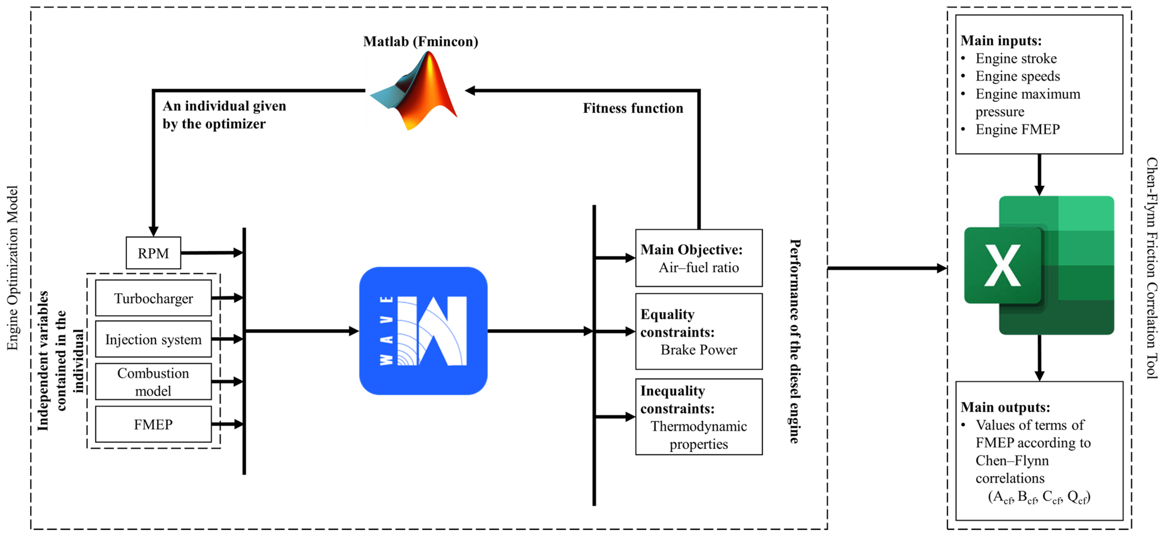
3.1. Overview of the Numerical Engine Model

The optimization model developed in this study integrates WAVE 2024.1 from Realis Simulation [53], as a 1D engine simulation software, with a nonlinear optimizer in Matlab, as shown in Figure 1. The results from the optimization model are subsequently imported into an Excel tool developed by Realis Simulation, which uses the Chen–Flynn model to fit the optimized data and determine the optimal coefficients for the friction equation.

The model has been developed to ensure high accuracy in engine calibration and to find the optimal values of the FMEP along the propeller curve. The engine model optimization finds the combination of the engine parameters, such as the turbocharger, injection system, and FMEP, to achieve a steady state at different operating points.

The model evaluates four specific operating points along the propeller curve to predict both the FMEP and maximum in-cylinder pressure: (1) rated power at 2100 rpm; (2) maximum and minimum speeds (1900 rpm and 1300 rpm) within the maximum torque range; and (3) the minimum engine speed at the propeller curve (600 rpm). The entire FMEP prediction process is conducted in liquid fuel mode, which is then used to compute the engine performance in both dual-fuel engine modes. Once the friction model’s coefficients are optimized, they can be applied directly to simulate any operating points along the engine load diagram. This approach enables more accurate friction prediction across varying load conditions and engine modes, providing a robust tool for evaluating engine performance.

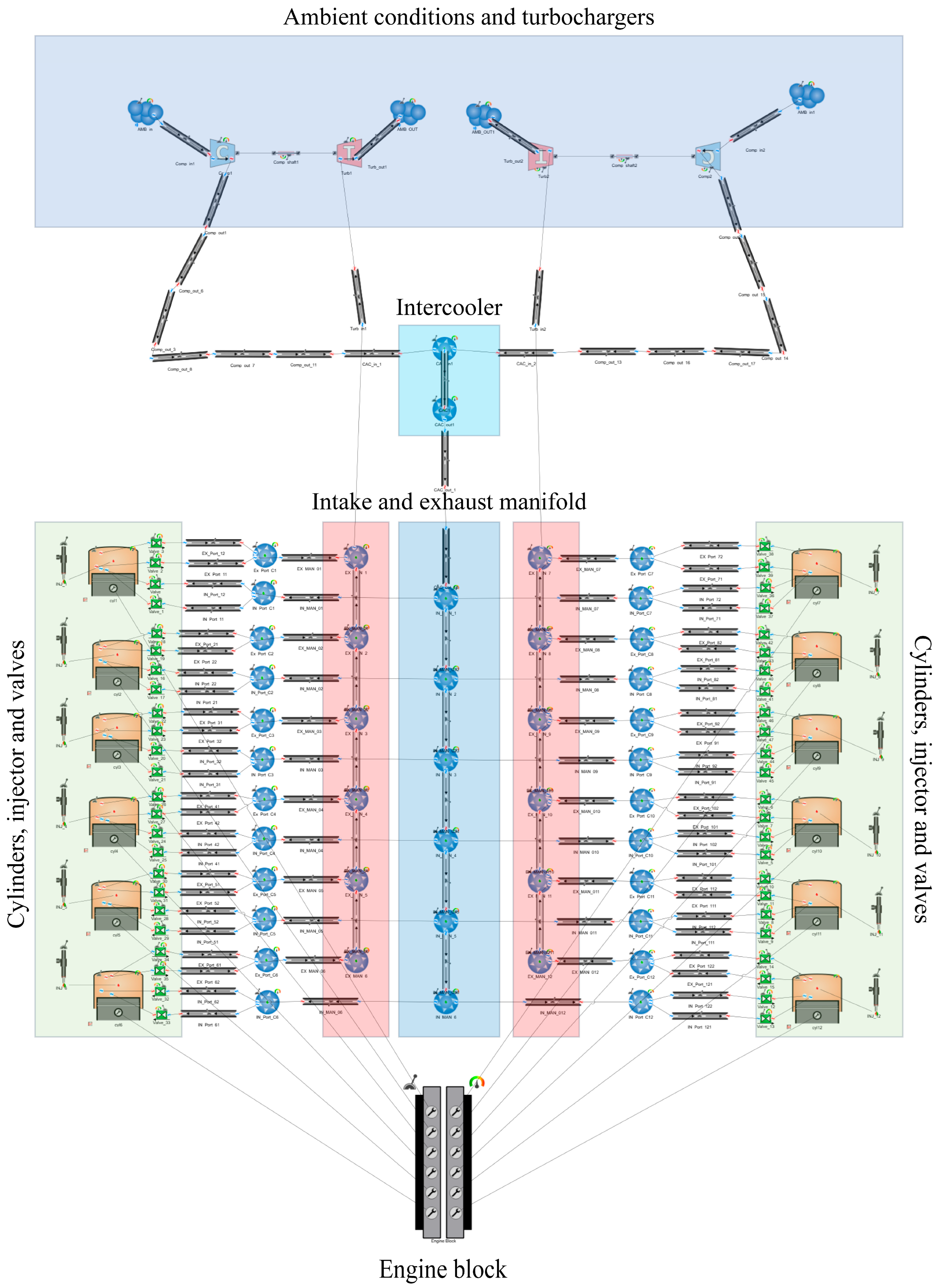
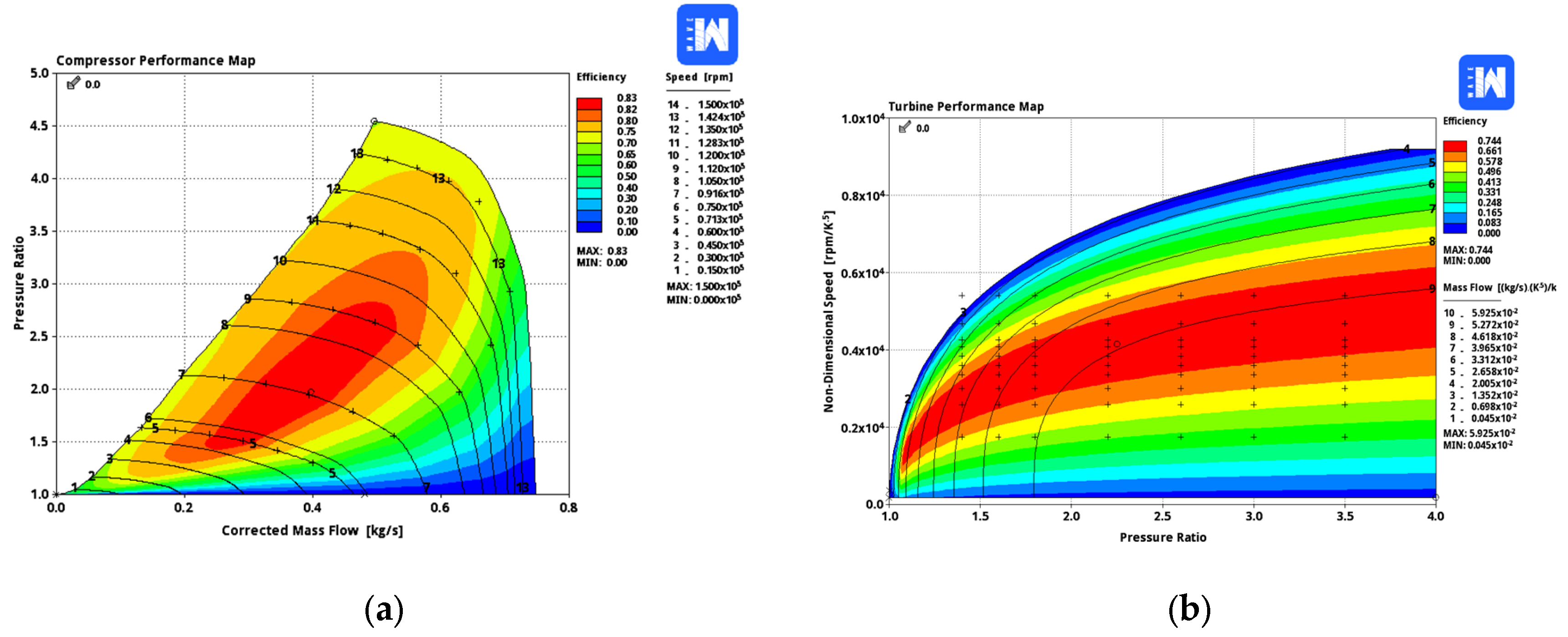
3.2. Description of WAVE Model

Firstly, the dual-fuel engine model is constructed in WAVE using the various elements available in the software, which combines flow, mechanical, and control components, as shown in Figure 2. The engine model features two turbochargers, one intercooler, twelve cylinders, and intake and exhaust manifolds. Similar to modern diesel engines, each cylinder is equipped with four valves—two for intake, two for exhaust—along with one injector in the liquid fuel mode, as the main focus of this study. The dimension of each part is collected from the project guide of the manufacturer [55,56].

The compressor and turbine maps for each turbocharger, as shown in Figure 3, are defined and rescaled from existing maps provided by the software to fit the engine’s needs for airflow at a given pressure.

The “filling and emptying” method is applied to control turbocharger performance and behavior using the energy and momentum equations recommended by Watson and Janota [57]. This approach treats each manifold or cylinder as a separate thermodynamic control volume, with its dynamics governed by energy and continuity equations as functions of time or crank angle.

Regarding the fuel injection system, the key parameters, including injection timing, profile, pressure, duration, and the injection rate within the cylinder, are considered during the simulation. The rectangular injection rate profile is selected as it is the common rate profile used due to its benefits in achieving a more stable combustion process as well as emissions reduction [58].

Cylinder processes are computed using the first law of thermodynamics [8], incorporating the heat release rate (HRR) during combustion [59,60], and heat transfer based on the empirical formula by Woschni [61].

The total heat added during the combustion process, dQ, as described in Equation (5), is computed for each crank angle. This calculation includes the heat released from fuel combustion, Q_comb, and the heat exchange, dQ_w, with the cylinder walls:

$${\mathrm{dQ}=\mathrm{Q}}_{\mathrm{comb}}{\mathrm{dx}}_{\mathrm{b}}{-\mathrm{dQ}}_{\mathrm{w}}$$

(5)

$${\mathrm{Q}}_{\mathrm{comb}}{=\mathrm{m}}_{\mathrm{fuel}}\mathrm{CV}$$

(6)

$${\mathrm{dQ}}_{\mathrm{w}}={\displaystyle \frac{{\mathrm{hA}}_{\mathrm{w}}}{\mathsf{\omega }}}{(\mathrm{T}}_{\mathrm{g}}{-\mathrm{T}}_{\mathrm{w}})\mathrm{d}\mathsf{\theta }$$

(7)

where m_fuel is the amount of injected fuel, CV is the calorific value of the injected fuel, h is the heat transfer coefficient suggested by Woschni, A_w is the area of cylinder walls, ω is the engine speed, T_g is the burn gas temperature, and T_w is the cylinder wall temperature.

The burned mass fraction, x_b, is computed using the equation suggested by Watson et al. [62], as expressed in Equation (8). This formula has been improved by the Realis Simulation team to consider the three phases of combustion. It is well-suited for combustion in the diesel cycle and does not require calibration, except for the reference speed (BRPM), as in Equation (9), to control the burn duration, unlike the single- and multi-Wiebe functions [63]. In some cases, the rated speed can be used as the reference speed [46,64]. The double-Wiebe function is introduced as an alternative to the single-Wiebe function to capture different phases of the combustion process better.

$${\mathrm{x}}_{\mathrm{b}}{=\mathrm{p}}_{\mathrm{f}}\left\{1-{\left[1-(0{.75\mathsf{\tau })}^2\right]}^{5000}\right\}{+\mathrm{d}}_{\mathrm{f}}\left\{1-{\left[{1-(\mathrm{cd}}_3{\mathsf{\tau })}^{1.75}\right]}^{5000}\right\}{+\mathrm{t}}_{\mathrm{f}}\left\{1-{\left[{1-(\mathrm{ct}}_3{\mathsf{\tau })}^{2.5}\right]}^{5000}\right\}$$

(8)

where p_f, d_f, and t_f are the mass fractions of the premix, diffusion, and tail burn curves, respectively. cd₃ and ct₃ are the burn duration coefficients for the diffusion and tail burn curves, respectively, and τ is the burn duration in degrees calculated according to the following expression:

$$\mathsf{\tau }={\displaystyle \frac{{\mathsf{\theta }-\mathsf{\theta }}_{\mathrm{o}}}{125{\left(\frac{\mathrm{RPM}}{\mathrm{BRPM}}\right)}^{0.3}}}$$

(9)

where θ is the crank angle, θ_o is the start angle of combustion, and RPM is the engine speed.

3.3. Nonlinear Optimizer

To enhance reproducibility and provide clarity on the implemented procedure, a flowchart of the MATLAB-based optimization algorithm is presented in Figure 4. The algorithm begins by defining the initial values and bounds for the key design variables.

These are passed into a nonlinear optimizer, which evaluates a fitness function aimed at maximizing the AFR while satisfying performance and combustion constraints, such as brake power, in-cylinder temperature, maximum pressure, and combustion stability (evaluated using R²). The nonlinear optimizer used in this study is the local optimizer “fmincon” based on an interior point algorithm [65] and integrated into Matlab. This optimizer has been selected due to its higher accuracy in achieving the optimal solution and lower computational time. The optimizer iteratively adjusts the variables, simulates the engine model in WAVE, and checks convergence until all constraints are met. The final output provides a set of optimized parameters for each operating condition. While it is a local optimizer, the computation can be performed more than once with an updated starting point to achieve the optimal solution and comply with all the constraints. However, the computational time is lower than that of a global optimizer like a genetic algorithm (GA) [66].

The main problem is defined to minimize the objective of the study and specified by the following equation:

$$\underset{\mathrm{x}}{\min }\hspace{0.17em}\mathrm{f}(\mathrm{x})\hspace{0.17em}\hspace{0.17em}\hspace{0.17em}\mathrm{such} \mathrm{that}\left\{\begin{array}{c}\mathrm{c}(\mathrm{x})\le 0\\ {\mathrm{c}}_{\mathrm{eq}}(\mathrm{x})=0\\ \mathrm{A}\cdot \mathrm{x}\le \mathrm{b}\\ {\mathrm{A}}_{\mathrm{eq}}\cdot \mathrm{x}={\mathrm{b}}_{\mathrm{eq}}\\ \mathrm{lb}\le \mathrm{x}\le \mathrm{ub}\end{array}\right.$$

(10)

where f(x) is the optimization model objective, c is the inequality constraints, c_eq is the equality constraints, A as a matrix and b as a vector are the linear inequality constraints, A_eq as a matrix and b_eq as a vector are the linear equality constraints, and lb and ub are the lower and upper bounds, respectively.

In this study, the main objective of the optimization problem is to maximize the AFR, unlike previous studies that minimize only the amount of fuel consumption [16,67,68]. Maximizing the AFR helps to not only reduce fuel consumption but also provides a sufficient amount of air, which improves the combustion process, increases the maximum in-cylinder pressure, reduces the maximum in-cylinder temperature, and thus reduces NO_x emissions. The optimization model assists in finding the optimal values of the different parameters along the engine parts with the known amount of the fuel rate (FR) collected from the project guide, such as the turbocharger speed (TS), start of injection (SOI), injection duration (INJ_Dur), FMEP, and BRPM. The design variables of the engine optimization model are presented by a five-dimensional vector x = (TS, SOI, INJ_Dur, FMEP, BRPM). The last design variable is optimized at the rated operating point and then kept constant while performing the optimization procedures at the partial operating points. The optimization problem is subjected to different equality and inequality constraints.

The main equality constraint of the optimization model is related to the engine brake power, PB, that needs to be achieved, as in Equation (11).

$${\mathrm{P}}_{\mathrm{B}}{ \left(\mathrm{x}\right)=\mathrm{P}}_{\mathrm{B}, \mathrm{obj}}$$

(11)

An additional equality constraint is considered only at the rated operating point, which is the known air mass flow rate, ṁ_a, inside the cylinders.

$${{\mathrm{m}}^{.}}_{\mathrm{a}} \left(\mathrm{x}\right)={{\mathrm{m}}^{.}}_{\mathrm{a}, \mathrm{obj}}$$

(12)

However, different inequality constraints are defined using the following expressions:

$${\mathrm{T}}_{\mathrm{AfterCylinder}}\left(\mathrm{x}\right)\le 1073\hspace{0.17em}\mathrm{K}$$

(13)

$${\mathrm{T}}_{\max }\left(\mathrm{x}\right)\le 1950\hspace{0.17em}\mathrm{K}$$

(14)

$${\mathrm{P}}_{\max }\left(\mathrm{x}\right)\le 180\hspace{0.17em}\mathrm{bar}$$

(15)

$$20\le \mathrm{AFR}\left(\mathrm{x}\right)\le 80$$

(16)

$${\mathrm{R}}^2\left(\mathrm{x}\right)\ge 0.99$$

(17)

where T_{AfterCylinder}(x) is the exhaust temperature after the cylinder in degree K, T_max(x) is the maximum average temperature inside the cylinder, and P_max(x) is the maximum in-cylinder pressure in bar.

The square of the coefficient of determination (R²) is used to evaluate the fuel burn rate along with the combustion duration compared to a polynomial equation from the sixth degree to ensure the smoothness of the curve and, thus, the combustion behavior, avoiding any misfire and unstable combustion. The degree of polynomial equations is selected based on several trials to ensure the best fitting. Due to the different values in the amount of fuel burn rate and the combustion duration, a normalized curve is presented, as shown in Figure 5. The fuel burn rate curve is rescaled from 0 to 1 to make it easier to identify, and the fitting procedures are performed.

These constraints are implemented into the optimization model by presenting them as a static penalty function, a degree of violation to make the absolute values less than one, as in the following expressions:

$${\mathrm{h}}_1\left(\mathrm{x}\right)={\displaystyle \frac{{\mathrm{P}}_{\mathrm{B}}}{{\mathrm{P}}_{\mathrm{B}, \mathrm{obj}}}}-1$$

(18)

$${\mathrm{h}}_2\left(\mathrm{x}\right)={\displaystyle \frac{{{\mathrm{m}}^{.}}_{\mathrm{a}}}{{{\mathrm{m}}^{.}}_{\mathrm{a}, \mathrm{obj}}}}-1$$

(19)

$${\mathrm{g}}_1\left(\mathrm{x}\right)={\displaystyle \frac{{\mathrm{T}}_{\mathrm{AfterCylinder}}}{{\mathrm{T}}_{\mathrm{AfterCylinder},\hspace{0.17em}\max }}}-1$$

(20)

$${\mathrm{g}}_2\left(\mathrm{x}\right)={\displaystyle \frac{{\mathrm{T}}_{\max }}{{\mathrm{T}}_{\max ,\hspace{0.17em}\max }}}-1$$

(21)

$${\mathrm{g}}_3\left(\mathrm{x}\right)={\displaystyle \frac{{\mathrm{P}}_{\max }}{{\mathrm{P}}_{\max ,\hspace{0.17em}\max }}}-1$$

(22)

$${\mathrm{g}}_4\left(\mathrm{x}\right)={\displaystyle \frac{\mathrm{AFR}}{{\mathrm{AFR}}_{\max }}}-1$$

(23)

$${\mathrm{g}}_5\left(\mathrm{x}\right)=-{\displaystyle \frac{\mathrm{AFR}}{{\mathrm{AFR}}_{\min }}}+1$$

(24)

$${\mathrm{g}}_6\left(\mathrm{x}\right)=-{\displaystyle \frac{{\mathrm{R}}^2}{{{\mathrm{R}}^2}_{\min }}}+1$$

(25)

The five optimization variables are subjected to specified ranges, as shown in the following equations:

$$5000\le \mathrm{TS}\le \mathrm{145,000}$$

(26)

$$-20\le \mathrm{SOI}\le 15$$

(27)

$$15\le {\mathrm{INJ}}_{\mathrm{Dur}}\le 35$$

(28)

$$0.8\le \mathrm{FMEP}\le 3$$

(29)

$$2100\le \mathrm{BRPM}\le 3000$$

(30)

where the range of the TS is defined according to the speed range of the compressor map, the ranges of the SOI, INJ_Dur, and FMEP are selected based on the common information of the diesel engines [69,70], and the range of the BRPM is defined according to the range suggested by the software.

In order to evaluate the performance of the optimization problem, the objective and both the equality and inequality constraints are implemented into a fitness function to achieve the minimum/maximum value of the objective and comply with all the constraints using the following equation:

$$\mathrm{Fitness}\hspace{0.17em}\mathrm{function}=\mathrm{AFR}\left(\mathrm{x}\right)+\mathrm{R}\left[{\displaystyle \sum _{\mathrm{i}=1}^{\mathrm{n}}\max \left(\mathrm{g}\right(\mathrm{x}),0)+{\displaystyle \sum _{\mathrm{j}=1}^{\mathrm{m}}\left|\mathrm{h}\left(\mathrm{x}\right)\right|}}\right]$$

(31)

where R is a constant equal to 1000 as previously used by [16,68].

4. Results and Discussions

4.1. Simulation of Marine Diesel Engine

Based on the developed optimization model, the engine’s performance is first computed and optimized at its rated power to identify the optimal combination of adjustable parameters such as the TS, SOI, FMEP, and INJ_Dur and a constant parameter such as the BRPM. The constant parameter is subsequently fixed while performing optimization at partial load conditions. This initial step serves as a calibration process, where critical factors such as air intake, fuel supply, exhaust temperature, and defined constraints significantly influence the determination of the optimal values for the adjustable variables.

To ensure accuracy and engine stability, each iteration involves simulating 40 cycles. Depending on the number of optimization variables involved, the simulation of each operating point takes approximately 4 to 8 h to reach optimal conditions.

The results, including the values of optimized variables, constraint parameters, and validation parameters, are presented in

Table 2. Computed results from the optimization model and percentage of error between real and simulation data at 100% rated power and 100% engine speed.

	Parameter	Unit	Real Value	Simulated Value	Percentage of Error [%]
Optimized variables	TS	[rpm]	-	131,529	-
	SOI	[BTDC]	-	−1.406	-
	INJDur	[degree]	-	32.98	-
	FMEP	[bar]	-	2.54	-
	BRPM	[rpm]	-	2957	-
Constraints parameters	TAfterCylinder	[K]	-	915	-
	Tmax	[K]	-	1771	-
	Pmax	[bar]	-	168.4	-
	AFR	[-]	-	26.2	-
	R2	[-]	-	0.9999	-
Validation parameters	PB	[kW]	749	748.74	0.034
	BSFC	[g/kW.h]	208	208	0
	ṁa	[kg/h]	4084	4082.56	0.035
	Texh	[K]	711	733	3.09

. These validation parameters quantify the percentage error between the manufacturer’s real-world data and the simulation results, ensuring the model’s accuracy and reliability.

Based on the optimized variables, the TS is adjusted at a higher engine speed to enhance airflow, resulting in a compressor efficiency of 78%, as derived from the performance maps. The SOI is optimized to occur a few degrees before the top dead center (TDC), with an injection duration of approximately 33°, ensuring high combustion pressure and a smooth, consistent fuel burn rate.

The FMEP is optimized at 2.54 bar, a value deemed appropriate for this type of diesel engine, balancing efficiency and reliability. The intake and exhaust valve lift ratios are carefully calculated, with the intake valve having a higher lift to maximize fresh air intake and improve the replacement of exhaust gases in the cylinder.

Additionally, the BRPM is set near the midpoint of its operational range, a critical factor in determining combustion duration and ensuring stable engine performance. These optimizations collectively contribute to enhanced engine efficiency and operational stability.

The constraint parameters adhere to the predefined safety limits, ensuring reliable engine operation. The P_max remains below 180 bar, while both the T_{AfterCylinder} and T_max are kept below their respective limits. This is achieved by maintaining a high air-to-fuel ratio within the cylinders, which not only enhances combustion efficiency but also significantly reduces NO_x emissions, ensuring compliance with IMO Tier II regulations.

Additionally, the R² for the fuel burn rate reaches an impressive 99.99%, indicating smooth and consistent combustion behavior throughout the process. This ensures optimal performance while meeting stringent emission standards.

To validate engine performance, key parameters—P_B, brake-specific fuel consumption (BSFC), air mass flow, and T_exh—are compared with real engine data. The first three parameters demonstrate excellent accuracy, with deviations of just 0.05%. The T_exh in the simulated results is slightly higher than the real data, with a deviation of 2.31%. This difference falls within an acceptable range and is likely attributed to the rescaling of existing performance maps to align with the characteristics of the current engine. These results confirm the reliability of the simulation model for engine performance evaluation.

After validating the engine model at the rated operating point, the optimized constant parameter values are used to simulate performance across three partial operating points. The same optimization methodology is applied to these reduced-variable cases, ensuring consistency and reliability in the approach. The computed results for all operating points are systematically summarized in

Table 3. Optimized engine parameters and corresponding combustion constraint values at three partial load points.

	Parameter	Unit	Case 1	Case 2	Case 3
	Engine speed	[rpm]	1900	1300	600
	Loading ratio	[%]	78.5	30.2	4.5
Optimized variables	TS	[rpm]	120,659	67,592	35,956
	SOI	[BTDC]	−3.69	−2.23	−1.69
	INJDur	[degree]	25.68	23.99	17.31
	FMEP	[bar]	2.48	1.86	1.17
Constraints parameters	TAfterCylinder	[K]	808	758	494
	Tmax	[K]	1717	1706	1334
	Pmax	[bar]	168.5	94.2	73.0
	AFR	[-]	30.19	31.03	68.89
	R2	[-]	0.9999	0.9998	0.9999

. These results show the adaptive behavior of the turbocharger speed, injection timing, and FMEP under varying engine speeds and loads. The increasing AFR at low load highlights the impact of reduced fuel demand, while consistently high R² values confirm combustion stability.

The TS decreases as the load is reduced, achieved by lowering the air supply and boosting pressure. The SOI is adjusted between 0° and −5° BTDC to ensure optimal combustion and achieve maximum in-cylinder pressure. At lower loads, the injection duration is shortened to account for the decreased cylinder combustion temperature and pressure, promoting smooth combustion. The AFR remains stable up to 31:1 for load ratios up to 30%, but it increases significantly at lower loads to enhance combustion efficiency. At 600 rpm, the engine operates at a very low load (4.5%), which results in a significantly reduced fuel injection quantity. However, the air supply remains comparatively high due to the turbocharger configuration and intake system dynamics. This imbalance leads to a high AFR of 68.89. While this value may appear high, such AFRs are typical during idle or low-load conditions in dual-fuel or lean-burn engines, where excess air improves combustion stability and reduces NO_x emissions. This behavior has been observed in similar low-load engine studies and is consistent with expected thermodynamic trends under minimal fueling scenarios.

The R² exceeds 0.9996, indicating smooth combustion with no misfires detected, ensuring reliable engine operation. The in-cylinder pressure diagram and fuel burn rate are presented in Figure 6, showing the reliability of the developed model in achieving smooth combustion at four different operating conditions with no misfire under all tested conditions.

4.2. Computation of the Terms of the Friction Model

Following the optimization and validation of the engine performance parameters across various load conditions, the next step involves refining the empirical friction model. This is achieved by fitting the optimized simulation results to the Chen–Flynn correlation to ensure accurate and scalable FMEP prediction.

To determine the coefficients of the Chen–Flynn correlation, the FMEP and the P_max at each engine speed are incorporated into the friction tool developed by the Realis Simulation team. Using the standard correlation coefficients presented in

Table 4. Comparison between the standard and optimized value of each term in Chen–Flynn correlation.

Term	Standard Value	Optimized Value
Acf	0.5	0.4309
Bcf	0.006	0.006
Ccf	600	655.3842
Qcf	0.2	0.2

as a baseline, the fitting process is executed with the friction tool to compute the percentage error between the calculated and predicted FMEP values for each engine speed. Initially, the percentage error remains within 7.2% across all speeds. However, to ensure high accuracy for subsequent simulations, it is necessary to minimize these errors further.

To refine the fitting process, the second and fourth terms of the Chen–Flynn correlation are retained as per the original equation, with fixed values of 0.006 and 0.2, respectively, while the first and third terms are computed based on the data defined in the Excel tool. B_cf and Q_cf are fixed to the standard literature values (0.006 and 0.2, respectively) due to their relatively low sensitivity to engine-specific variations and the absence of reliable experimental data to refine them. These terms predominantly capture baseline friction behavior associated with pressure and velocity effects that are consistent across engine types. In contrast, A_cf and C_cf are treated as variable terms and optimized using the friction fitting tool, as they are more influenced by the specific design and operational characteristics of the engine (e.g., surface finish, lubrication, piston speed). This approach strikes a balance between modeling accuracy and practical constraints, ensuring that the refined coefficients accurately reflect the real behavior of the studied engine while maintaining computational efficiency.

Adjustments are made by replacing the computed FMEP values with the predicted ones from the fitting model at engine speeds through multiple iterations. This iterative refinement is repeated across the speed range, starting with the points with a higher percentage of errors, until achieving a stable and improved R² between the calculated and predicted FMEP curves. This method ensures enhanced accuracy and reliability of the correlation for future applications.

Figure 7 illustrates the strong correlation between the newly computed values and the predicted FMEP values, demonstrating the effectiveness of the fitting process. The final R² value between the two curves is 0.9999, indicating a nearly perfect match. The percentage error across the engine speeds ranges from 0.13% to −0.13%, reflecting a significant reduction in discrepancies and ensuring high accuracy of the model across varying operating conditions. Table 4 shows the new values of each term compared to the standard values.

Comparable studies using empirical fitting techniques and numerical optimization also report R² values above 0.98 for friction prediction models [71,72], which supports the validity of our results given the controlled simulation environment and absence of experimental noise.

After incorporating the updated coefficient values into the Chen–Flynn correlation, minor deviations, such as those presented in the computed results in Table 3, are to be expected. These discrepancies arise due to the sensitivity of the correlation to changes in its parameters, especially when applied to complex thermodynamic systems. Nevertheless, the overall trends remain consistent, and the observed variations fall within acceptable error margins for engineering applications. Additionally, the performance of the engine at various operating conditions along the engine load diagram will be calculated.

5. Conclusions and Further Research

This study proposes an optimization method to predict the optimal coefficients of the Chen–Flynn correlation, employing advanced optimization techniques to accurately calculate the FMEP for a given engine, even in the absence of real data.

The approach integrates a 1D engine simulation software with a nonlinear optimization algorithm implemented in MATLAB, creating a robust engine optimization model. This model predicts engine performance while determining the optimal values of critical parameters governing engine behavior across four operating points. Key outputs, including engine speed, FMEP, and P_max, are then incorporated into a specialized friction tool for data fitting and validation.

The following has been concluded:

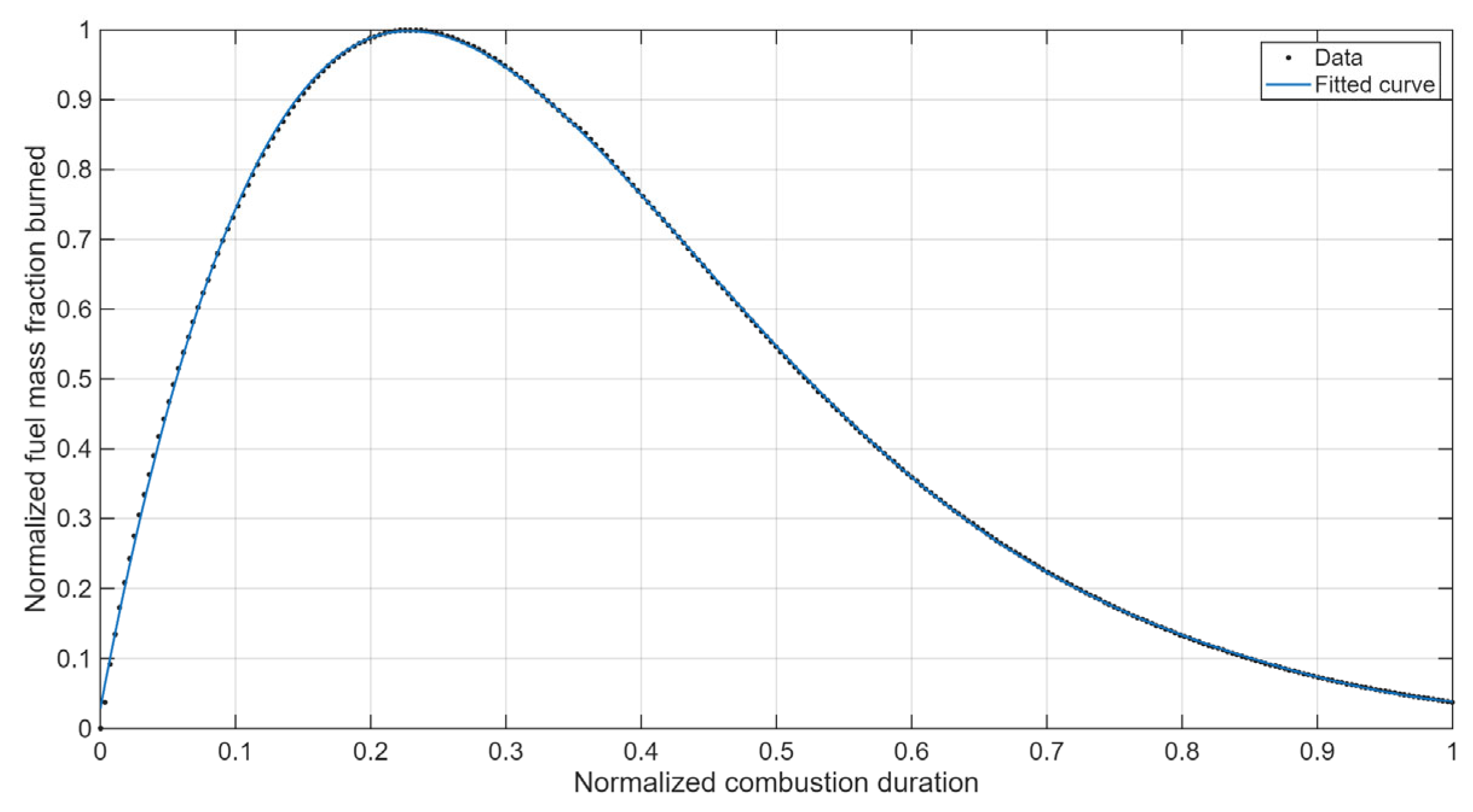
• The engine model facilitates maximizing the AFR by optimizing the turbocharger performance, injection system parameters, combustion characteristics, and the FMEP. This results in values of up to 68.89 at low-load operation, while maintaining combustion stability (R² ≥ 0.9998).
• The engine optimization model demonstrates excellent capability in meeting all predefined constraints, ensuring reliability and applicability under varying conditions.
• The numerical model is computationally efficient and compatible with standard computer systems, offering fast simulation times while maintaining high accuracy in calculated results. It helps to match real engine performance with an error of less than 0.05% in brake power and BSFC, confirming both accuracy and efficiency.
• The developed approach supports the precise determination of the Chen–Flynn correlation coefficients, enhancing the accuracy of engine performance predictions across the load diagram.

This methodology provides a reliable approach to assessing engine friction behavior, particularly in scenarios where manufacturer-specific data is unavailable. These findings validate the model as a powerful tool for practical engine performance assessment and support its integration into advanced digital twin frameworks for marine propulsion systems.

Future work could explore the performance simulation of dual-fuel engines operating with hydrogen as the primary fuel. Additionally, incorporating a life-cycle assessment (LCA) of emissions can help evaluate the full environmental impact of dual-fuel engines, particularly when transitioning to hydrogen-based fuels. This would provide a more comprehensive comparison between fuel options and support decision-making for sustainable marine propulsion. While this study focuses on steady-state operation, evaluating the model’s performance under transient conditions, such as acceleration, deceleration, and load fluctuations, would further enhance its robustness and applicability to real-world marine engine operations. Incorporating transient simulations could also aid in control system development and engine calibration strategies.

Such research aligns with global efforts toward net-zero emissions, positioning hydrogen as a key enabler of sustainable maritime and automotive propulsion systems.

References

1. Tadros, M.; Ventura, M.; Guedes Soares, C. Review of the IMO Initiatives for Ship Energy Efficiency and Their Implications. J. Mar. Sci. Appl. 2023, 22, 662–680. [Google Scholar] [CrossRef]
2. Theotokatos, G.; Stoumpos, S.; Bolbot, V.; Boulougouris, E. Simulation-based investigation of a marine dual-fuel engine. J. Mar. Eng. Technol. 2020, 19, 5–16. [Google Scholar] [CrossRef]
3. IMO. EEXI and CII-Ship Carbon Intensity and Rating System. Available online: https://www.imo.org/en/MediaCentre/HotTopics/Pages/EEXI-CII-FAQ.aspx (accessed on 10 November 2022).
4. Karatuğ, Ç.; Ejder, E.; Tadros, M.; Arslanoğlu, Y. Environmental and Economic Evaluation of Dual-Fuel Engine Investment of a Container Ship. J. Mar. Sci. Appl. 2023, 22, 823–836. [Google Scholar] [CrossRef]
5. Tauzia, X.; Maiboom, A.; Karaky, H.; Chesse, P. Experimental analysis of the influence of coolant and oil temperature on combustion and emissions in an automotive diesel engine. Int. J. Engine Res. 2019, 20, 247–260. [Google Scholar] [CrossRef]
6. Jia, B.; Mikalsen, R.; Smallbone, A.; Roskilly, A.P. A study and comparison of frictional losses in free-piston engine and crankshaft engines. Appl. Therm. Eng. 2018, 140, 217–224. [Google Scholar] [CrossRef]
7. Karatuğ, Ç.; Ceylan, B.O.; Arslanoğlu, Y. A hybrid predictive maintenance approach for ship machinery systems: A case of main engine bearings. J. Mar. Eng. Technol. 2025, 24, 12–21. [Google Scholar] [CrossRef]
8. Heywood, J.B. Internal Combustion Engine Fundamentals; McGraw-Hill: New York, NY, USA, 1988. [Google Scholar]
9. Tadros, M.; Ventura, M.; Guedes Soares, C. Review of current regulations, available technologies, and future trends in the green shipping industry. Ocean. Eng. 2023, 280, 114670. [Google Scholar] [CrossRef]
10. Huang, Y.; Surawski, N.C.; Zhuang, Y.; Zhou, J.L.; Hong, G. Dual injection: An effective and efficient technology to use renewable fuels in spark ignition engines. Renew. Sustain. Energy Rev. 2021, 143, 110921. [Google Scholar] [CrossRef]
11. Sander, D.E.; Knauder, C.; Allmaier, H.; Damjanović-Le Baleur, S.; Mallet, P. Friction Reduction Tested for a Downsized Diesel Engine with Low-Viscosity Lubricants Including a Novel Polyalkylene Glycol. Lubricants 2017, 5, 9. [Google Scholar] [CrossRef]
12. Feneley, A.J.; Pesiridis, A.; Andwari, A.M. Variable Geometry Turbocharger Technologies for Exhaust Energy Recovery and Boosting-A Review. Renew. Sustain. Energy Rev. 2017, 71, 959–975. [Google Scholar] [CrossRef]
13. Cong, Y.; Gan, H.; Wang, H. Parameter investigation of the pilot fuel post-injection strategy on performance and emissions characteristics of a large marine two-stroke natural gas-diesel dual-fuel engine. Fuel 2022, 323, 124404. [Google Scholar] [CrossRef]
14. Xiang, L.; Theotokatos, G.; Ding, Y. Parametric investigation on the performance-emissions trade-off and knocking occurrence of dual fuel engines using CFD. Fuel 2023, 340, 127535. [Google Scholar] [CrossRef]
15. Bejger, A.; Chybowski, L.; Gawdzińska, K. Utilising elastic waves of acoustic emission to assess the condition of spray nozzles in a marine diesel engine. J. Mar. Eng. Technol. 2018, 17, 153–159. [Google Scholar] [CrossRef]
16. Tadros, M.; Ventura, M.; Guedes Soares, C. Optimization procedure to minimize fuel consumption of a four-stroke marine turbocharged diesel engine. Energy 2019, 168, 897–908. [Google Scholar] [CrossRef]
17. Wei, S.; Wu, C.; Yan, S.; Ding, T.; Chen, J. Miller Cycle with Early Intake Valve Closing in Marine Medium-Speed Diesel Engines. J. Mar. Sci. Appl. 2022, 21, 151–160. [Google Scholar] [CrossRef]
18. Kim, J.; Vallinmaki, M.; Tuominen, T.; Mikulski, M. Variable valve actuation for efficient exhaust thermal management in an off-road diesel engine. Appl. Therm. Eng. 2024, 246, 122940. [Google Scholar] [CrossRef]
19. Güler, M.; Özkan, M. Energy balance analysis of a DI diesel engine with multiple pilot injections strategy and optimization of brake thermal efficiency. Appl. Therm. Eng. 2022, 204, 117972. [Google Scholar] [CrossRef]
20. Singh, D.; Gu, F.; Fieldhouse, J.D.; Singh, N.; Singal, S.K. Prediction and Analysis of Engine Friction Power of a Diesel Engine Influenced by Engine Speed, Load, and Lubricant Viscosity. Adv. Tribol. 2014, 2014, 928015. [Google Scholar] [CrossRef]
21. Allmaier, H.; Knauder, C.; Salhofer, S.; Reich, F.; Schalk, E.; Ofner, H.; Wagner, A. An experimental study of the load and heat influence from combustion on engine friction. Int. J. Engine Res. 2016, 17, 347–353. [Google Scholar] [CrossRef]
22. Spencer, A.; Avan, E.Y.; Almqvist, A.; Dwyer-Joyce, R.S.; Larsson, R. An experimental and numerical investigation of frictional losses and film thickness for four cylinder liner variants for a heavy duty diesel engine. Proc. Inst. Mech. Eng. Part J. 2013, 227, 1319–1333. [Google Scholar] [CrossRef]
23. Li, R.; Wen, C.; Meng, X.; Xie, Y. Measurement of the friction force of sliding friction pairs in low-speed marine diesel engines and comparison with numerical simulation. Appl. Ocean. Res. 2022, 121, 103089. [Google Scholar] [CrossRef]
24. Chybowski, L.; Kowalak, P.; Dąbrowski, P. Assessment of the Impact of Lubricating Oil Contamination by Biodiesel on Trunk Piston Engine Reliability. Energies 2023, 16, 5056. [Google Scholar] [CrossRef]
25. Mujtaba, M.A.; Masjuki, H.H.; Kalam, M.A.; Noor, F.; Farooq, M.; Ong, H.C.; Gul, M.; Soudagar, M.E.M.; Bashir, S.; Rizwanul Fattah, I.M.; et al. Effect of Additivized Biodiesel Blends on Diesel Engine Performance, Emission, Tribological Characteristics, and Lubricant Tribology. Energies 2020, 13, 3375. [Google Scholar] [CrossRef]
26. Mosarof, M.H.; Kalam, M.A.; Masjuki, H.H.; Alabdulkarem, A.; Habibullah, M.; Arslan, A.; Monirul, I.M. Assessment of friction and wear characteristics of Calophyllum inophyllum and palm biodiesel. Ind. Crops Prod. 2016, 83, 470–483. [Google Scholar] [CrossRef]
27. Tiruvenkadam, N.; Thyla, P.R.; Senthilkumar, M.; Bharathiraja, M. Development of optimum friction new nano hybrid composite liner for biodiesel fuel engine. Transp. Res. Part D Transp. Environ. 2016, 47, 22–43. [Google Scholar] [CrossRef]
28. Thangarasu, V.; Balaji, B.; Ramanathan, A. Experimental investigation of tribo-corrosion and engine characteristics of Aegle Marmelos Correa biodiesel and its diesel blends on direct injection diesel engine. Energy 2019, 171, 879–892. [Google Scholar] [CrossRef]
29. Singh, P.; Goel, V.; Chauhan, S.R. Impact of dual biofuel approach on engine oil dilution in CI engines. Fuel 2017, 207, 680–689. [Google Scholar] [CrossRef]
30. Mousavi, S.B.; Zeinali Heris, S.; Estellé, P. Viscosity, tribological and physicochemical features of ZnO and MoS2 diesel oil-based nanofluids: An experimental study. Fuel 2021, 293, 120481. [Google Scholar] [CrossRef]
31. Dey, S.; Moni Reang, N.; Deb, M.; Kumar Das, P. Experimental investigation on combustion-performance-emission characteristics of nanoparticles added biodiesel blends and tribological behavior of contaminated lubricant in a diesel engine. Energy Convers. Manag. 2021, 244, 114508. [Google Scholar] [CrossRef]
32. Kapłan, M.; Klimek, K.; Maj, G.; Zhuravel, D.; Bondar, A.; Lemeshchenko-Lagoda, V.; Boltianskyi, B.; Boltianska, L.; Syrotyuk, H.; Syrotyuk, S.; et al. Method of Evaluation of Materials Wear of Cylinder-Piston Group of Diesel Engines in the Biodiesel Fuel Environment. Energies 2022, 15, 3416. [Google Scholar] [CrossRef]
33. Abril, S.O.; García, C.P.; León, J.P. Numerical and Experimental Analysis of the Potential Fuel Savings and Reduction in CO Emissions by Implementing Cylinder Bore Coating Materials Applied to Diesel Engines. Lubricants 2021, 9, 19. [Google Scholar] [CrossRef]
34. Lyu, B.; Meng, X.; Wang, C.; Cui, Y.; Wang, C.e. Piston ring and cylinder liner scuffing analysis in dual-fuel low-speed engines considering liner deformation and tribofilm evolution. Int. J. Engine Res. 2024, 25, 1776–1798. [Google Scholar] [CrossRef]
35. Albrecht, A.; Grondin, O.; Le Berr, F.; Le Solliec, G. Towards a Stronger Simulation Support for Engine Control Design: A Methodological Point of View. Oil Gas Sci. Technol. 2007, 62, 437–456. [Google Scholar] [CrossRef]
36. Wei, S.; Zhao, X.; Liu, X.; Qu, X.; He, C.; Leng, X. Research on effects of early intake valve closure (EIVC) miller cycle on combustion and emissions of marine diesel engines at medium and low loads. Energy 2019, 173, 48–58. [Google Scholar] [CrossRef]
37. AVL. AVL-Development, Testing & Simulation of Powertrain Systems. Available online: https://www.avl.com/ (accessed on 4 October 2017).
38. Mocerino, L.; Guedes Soares, C.; Rizzuto, E.; Balsamo, F.; Quaranta, F. Validation of an Emission Model for a Marine Diesel Engine with Data from Sea Operations. J. Mar. Sci. Appl. 2021, 20, 534–545. [Google Scholar] [CrossRef]
39. Ricardo Wave Software, WAVE 2019.1 Help System; Ricardo plc: Shoreham-by-Sea, UK, 2019.
40. Shen, H.; Yang, F.; Jiang, D.; Lu, D.; Jia, B.; Liu, Q.; Zhang, X. Parametric Investigation on the Influence of Turbocharger Performance Decay on the Performance and Emission Characteristics of a Marine Large Two-Stroke Dual Fuel Engine. J. Mar. Sci. Eng. 2024, 12, 1298. [Google Scholar] [CrossRef]
41. Gamma Technologies LLC. GT-POWER Engine Simulation Software. Available online: https://www.gtisoft.com/gt-suite-applications/propulsion-systems/gt-power-engine-simulation-software/ (accessed on 4 October 2017).
42. Stoumpos, S.; Theotokatos, G.; Mavrelos, C.; Boulougouris, E. Towards Marine Dual Fuel Engines Digital Twins—Integrated Modelling of Thermodynamic Processes and Control System Functions. J. Mar. Sci. Eng. 2020, 8, 200. [Google Scholar] [CrossRef]
43. Karatuğ, Ç.; Tadros, M.; Ventura, M.; Guedes Soares, C. Decision support system for ship energy efficiency management based on an optimization model. Energy 2024, 292, 130318. [Google Scholar] [CrossRef]
44. Tadros, M.; Ventura, M.; Guedes Soares, C. A nonlinear optimization tool to simulate a marine propulsion system for ship conceptual design. Ocean. Eng. 2020, 210, 107417. [Google Scholar] [CrossRef]
45. Tadros, M.; Ventura, M.; Guedes Soares, C. Surrogate models of the performance and exhaust emissions of marine diesel engines for ship conceptual design. In Maritime Transportation and Harvesting of Sea Resources; Guedes Soares, C., Teixeira, A.P., Eds.; Taylor & Francis Group: London, UK, 2018; pp. 105–112. [Google Scholar]
46. Tadros, M.; Ventura, M.; Guedes Soares, C. Data Driven In-Cylinder Pressure Diagram Based Optimization Procedure. J. Mar. Sci. Eng. 2020, 8, 294. [Google Scholar] [CrossRef]
47. Kolakoti, A.; Tadros, M.; Ambati, V.K.; Gudlavalleti, V.N.S. Optimization of biodiesel production, engine exhaust emissions, and vibration diagnosis using a combined approach of definitive screening design (DSD) and artificial neural network (ANN). Environ. Sci. Pollut. Res. 2023, 30, 87260–87273. [Google Scholar] [CrossRef]
48. ASTM D6751-24; Standard Specification for Biodiesel Fuel Blendstock (B100) for Middle Distillate Fuels. ASTM: West Conshohocken, PA, USA, 2024.
49. Chen, S.K.; Flynn, P.F. Development of Single Cylinder Compression Ignition Research Engine; SAE Technical Paper; SAE: Warrendale, PA, USA, 1965. [Google Scholar] [CrossRef]
50. Tormos, B.; Martín, J.; Blanco-Cavero, D.; Jiménez-Reyes, A.J. One-Dimensional Modeling of Mechanical and Friction Losses Distribution in a Four-Stroke Internal Combustion Engine. J. Tribol. 2020, 142, 011703. [Google Scholar] [CrossRef]
51. Chen, Y.; Deng, B.; Chen, M.; Hou, K. An approach to estimate CCV (cycle-to-cycle variation) of effective energy output of thermal engine: A case study on a high speed gasoline engine. Case Stud. Therm. Eng. 2021, 28, 101624. [Google Scholar] [CrossRef]
52. Özgül, E.; Bedir, H. Fast NOx emission prediction methodology via one-dimensional engine performance tools in heavy-duty engines. Adv. Mech. Eng. 2019, 11, 1687814019845954. [Google Scholar] [CrossRef]
53. Realis Simulation, WAVE 2024.1 Help System; Realis Simulation: Shoreham-by-Sea, UK, 2024.
54. MAN Diesel & Turbo. Four-Stroke Project Guides. Available online: https://www.man-es.com/marine/products/planning-tools-and-downloads/project-guides/four-stroke (accessed on 22 July 2022).
55. MAN Diesel & Turbo. Technical Data Sheet: Marine Diesel Engine D2862 LE428. Available online: https://www.man.eu/ntg_media/media/content_medien/doc/man_engines_1/produkte/marine_1/Marine_DualFuel_EN.pdf (accessed on 15 April 2023).
56. OEM Off-Highway. MAN Updates Engine Portfolio for Stage IV and Tier 4 Final Construction Machinery. Available online: https://www.oemoffhighway.com/engines/press-release/12163906/man-updates-engine-portfolio-for-stage-iv-and-tier-4-final-construction-machinery (accessed on 15 April 2020).
57. Watson, N.; Janota, M.S. Turbocharging the Internal Combustion Engine; Palgrave: London, UK, 1982. [Google Scholar]
58. Bai, F.; Zhang, Z.; Du, Y.; Zhang, F.; Peng, Z. Effects of Injection Rate Profile on Combustion Process and Emissions in a Diesel Engine. J. Combust. 2017, 2017, 9702625. [Google Scholar] [CrossRef]
59. Maroteaux, F.; Saad, C. Diesel engine combustion modeling for hardware in the loop applications: Effects of ignition delay time model. Energy 2013, 57, 641–652. [Google Scholar] [CrossRef]
60. Maroteaux, F.; Saad, C.; Aubertin, F. Development and validation of double and single Wiebe function for multi-injection mode Diesel engine combustion modelling for hardware-in-the-loop applications. Energy Convers. Manag. 2015, 105, 630–641. [Google Scholar] [CrossRef]
61. Woschni, G. A Universally Applicable Equation for the Instantaneous Heat Transfer Coefficient in the Internal Combustion Engine; SAE Technical Paper; SAE: Warrendale, PA, USA, 1967. [Google Scholar]
62. Watson, N.; Pilley, A.D.; Marzouk, M. A Combustion Correlation for Diesel Engine Simulation; SAE: Warrendale, PA, USA, 1980; Volume SAE Paper 800029. [Google Scholar]
63. Tadros, M.; Ventura, M.; Guedes Soares, C. Assessment of the performance and the exhaust emissions of a marine diesel engine for different start angles of combustion. In Maritime Technology and Engineering 3; Guedes Soares, C., Santos, T.A., Eds.; Taylor & Francis Group: London, UK, 2016; pp. 769–775. [Google Scholar]
64. Tadros, M.; Ventura, M.; Guedes Soares, C. Simulation of the performance of marine Genset based on double-Wiebe function. In Sustainable Development and Innovations in Marine Technologies; Georgiev, P., Guedes Soares, C., Eds.; Taylor & Francis Group: London, UK, 2020; pp. 292–299. [Google Scholar]
65. Byrd, R.H.; Mary, E.H.; Nocedal, J. An Interior Point Algorithm for Large-Scale Nonlinear Programming. SIAM J. Optim. 1999, 9, 877–900. [Google Scholar] [CrossRef]
66. The MathWorks Inc. Fmincon. Available online: https://www.mathworks.com/help/optim/ug/fmincon.html (accessed on 2 June 2017).
67. Zhu, Z.; Zhang, F.; Li, C.; Wu, T.; Han, K.; Lv, J.; Li, Y.; Xiao, X. Genetic algorithm optimization applied to the fuel supply parameters of diesel engines working at plateau. Appl. Energy 2015, 157, 789–797. [Google Scholar] [CrossRef]
68. Zhao, J.; Xu, M. Fuel economy optimization of an Atkinson cycle engine using genetic algorithm. Appl. Energy 2013, 105, 335–348. [Google Scholar] [CrossRef]
69. Challen, B.; Baranescu, R. Diesel Engine Reference Book, 2nd ed.; Challen, B., Baranescu, R., Eds.; Butterworth-Heinemann Ltd.: Oxford, UK, 1999. [Google Scholar]
70. Woodyard, D. Pounder’s Marine Diesel Engines, 8th ed.; Butterworth-Heinemann: Oxford, UK, 2004. [Google Scholar]
71. Tormos, B.; Martín, J.; Pla, B.; Jiménez-Reyes, A.J. A methodology to estimate mechanical losses and its distribution during a real driving cycle. Tribol. Int. 2020, 145, 106208. [Google Scholar] [CrossRef]
72. Chen, R.; Zhao, B.; He, T.; Tu, L.; Xie, Z.; Zhong, N.; Zou, D. Study on coupling transient mixed lubrication and time-varying wear of main bearing in actual operation of low-speed diesel engine. Tribol. Int. 2024, 191, 109159. [Google Scholar] [CrossRef]
Figure 1. Overview of the developed optimization model for FMEP prediction.
Algorithms 18 00415 g001
Figure 2. Layout of the 1D engine model implemented in WAVE.
Algorithms 18 00415 g002
Figure 3. Maps of (a) compressor and (b) turbine of the installed turbocharger used in the simulation.
Algorithms 18 00415 g003
Figure 4. Schematic diagram of the engine optimization model.
Algorithms 18 00415 g004
Figure 5. Fitting procedure of the normalized fuel mass fraction burned.
Algorithms 18 00415 g005
Figure 6. (a) In-cylinder pressure diagram and (b) fuel burn rate for four different engine operating points.
Algorithms 18 00415 g006
Figure 7. Fitting curve of FMEP.
Algorithms 18 00415 g007