Article

Inspiring from Galaxies to Green AI in Earth: Benchmarking Energy-Efficient Models for Galaxy Morphology Classification

by
Vasileios Alevizos
1,2,
Emmanouil V. Gkouvrikos
1,
Ilias Georgousis
1,
Sotiria Karipidou
1 and
George A. Papakostas
1,*
1
MLV Research Group, Department of Informatics, Democritus University of Thrace, 65404 Kavala, Greece
2
Karolinska Institutet, Department of Learning, Informatics, Management and Ethics, 17176 Solna, Sweden
*
Author to whom correspondence should be addressed.
Algorithms 2025, 18(7), 399; https://doi.org/10.3390/a18070399
Submission received: 4 May 2025 / Revised: 23 June 2025 / Accepted: 25 June 2025 / Published: 28 June 2025
(This article belongs to the Special Issue Artificial Intelligence in Space Applications)

Abstract

Recent advancements in space exploration have significantly increased the volume of astronomical data, heightening the demand for efficient analytical methods. Concurrently, the considerable energy consumption of machine learning (ML) has fostered the emergence of Green AI, emphasizing sustainable, energy-efficient computational practices. We introduce the first large-scale Green AI benchmark for galaxy morphology classification, evaluating over 30 machine learning architectures (classical, ensemble, deep, and hybrid) on CPU and GPU platforms using a balanced subset of the Galaxy Zoo dataset. Beyond traditional metrics (precision, recall, and F1-score), we quantify inference latency, energy consumption, and carbon-equivalent emissions to derive an integrated EcoScore that captures the trade-off between predictive performance and environmental impact. Our results reveal that a GPU-optimized multilayer perceptron achieves state-of-the-art accuracy of 98% while emitting 20× less CO2 than ensemble forests, which—despite comparable accuracy—incur substantially higher energy costs. We demonstrate that hardware–algorithm co-design, model sparsification, and careful hyperparameter tuning can reduce carbon footprints by over 90% with negligible loss in classification quality. These findings provide actionable guidelines for deploying energy-efficient, high-fidelity models in both ground-based data centers and onboard space observatories, paving the way for truly sustainable, large-scale astronomical data analysis.

1. Introduction

The foundational investigation into galaxy morphology significantly contributes to the discourse surrounding processes responsible for cosmic formation and evolution. Nevertheless, accurately categorizing galaxies by their morphological features presents substantial challenges due to diverse classifications, ambiguities in visual interpretation, and the complexity of galactic images themselves [1]. This complexity stems primarily from diverse physical circumstances and environmental interactions experienced by celestial bodies, culminating in a broad spectrum of structural characteristics and morphological indicators.
The continual advancement in observational technology, including more powerful telescopes and sophisticated instruments, has exponentially increased the volume of astronomical data. Consequently, astronomers possess extensive image datasets that, although valuable for in-depth analyses, introduce significant issues regarding the management and accuracy of data interpretation as well as the leaving carbon footprint [2]. Manual classification of these extensive datasets has revealed itself as inefficient and prone to inconsistencies [3].
To overcome the described limitations inherent in manual image classification, previous propositions have suggested automating this procedure through the employment of advanced machine learning methodologies. Particularly noteworthy among these methods is the convolutional neural network (CNN), extensively employed in image-based analyses. Despite successes, pre-existing publicly accessible datasets display limitations, notably the absence of various galaxy categories and the presence of low-quality imaging data, consequently restricting CNN model generalizability. Additionally, classification and precise localization of celestial objects require balancing model granularity with generalization capacity.
In response to these outlined challenges, this study is conducted through a logical progression of methodological steps. Initially, multiple models, along with CNN models, are designated for evaluation, aiming to examine their capability in accurately classifying astronomical imagery obtained from the Galaxy Zoo dataset [4]. The evaluation phase involves determining several performance diagnostics, monitoring not only the performance but also computational fluctuations over temperature. These metrics are indicators of model efficiency, effectiveness, sustainability, and applicability in embedded computing systems. This selection of diagnostics embraces the concept of Green AI (Artificial Intelligence) by pondering energy efficiency and minimal environmental impact.
Simultaneously, emerging developments in computational technology have inspired collaborative projects between public organizations and leading corporations. These collaborations pursue sophisticated algorithmic solutions that address complex space-science objectives, including asteroid detection and the search for extraterrestrial life. NASA particularly employs advanced ML techniques designed to detect rare biological signatures within massive data quantities gathered from next-generation telescopes [5,6].
From these investigative circumstances emerge essential research inquiries. Primarily, can existing pre-trained CNN models effectively analyze astronomical image datasets? Moreover, among the tested models, which demonstrate superior performance across specified performance metrics? Lastly, the present investigation proposes future enhancements to datasets, enabling subsequent evaluations of the identified top-performing models. Addressing these questions provides a reliable benchmark and facilitates insights regarding automated analysis efficacy, potentially augmenting exploration accuracy within astronomy and refining navigation capabilities in space exploration contexts.
The structure of this paper is organized to ensure a systematic presentation of research methodology, analytical techniques, and experimental steps, as well as the obtained outcomes. Initially, existing state-of-the-art ML and deep learning (DL) models are surveyed for their performance on classification tasks. This analysis evaluates recent advancements within space object categorization, assessing relative merits alongside limitations inherent in each method. Subsequently, theoretical backgrounds pertinent to selected analytical methodologies are provided. This segment addresses fundamental principles influencing method selection, articulating reasoning aligned with identified research gaps. Motivation underlying the study originates from unresolved classification and localization challenges present in prior scholarly research, which justify novel exploration. Next, the development of experimental procedures is outlined, encompassing dataset preprocessing, feature engineering, model selection, hyperparameter tuning, validation strategies, and performance evaluation metrics. Afterward, the results derived from implementing these procedures upon the Galaxy Zoo dataset are systematically interpreted in relation to predefined research objectives, offering comparative analyses against prior benchmarks. This section articulates implications emerging from empirical evidence while identifying constraints encountered throughout methodological applications. Limitations discovered during experimentation receive careful attention, facilitating consideration for subsequent research avenues within astronomical object classification employing ML methodologies.

1.1. Green AI

The domain of Green autonomous models has experienced substantial growth in recent years due to ecological concerns associated with them. Established analysis of the literature [7] indicates a considerable increase in scholarly attention to this domain. Studies within the Green AI literature generally encompass observational, solution-based, and positional methodologies. These categories involve tasks such as environmental monitoring of AI models, hyperparameter tuning aimed at sustainability, model benchmarking, deployment strategies, and other relevant activities. Investigations of the efficiency of AI models have indicated potential energy savings [8,9]. Consequently, the AI research community has gradually integrated sustainability goals within the core principles of development processes. Within this framework, sustainable practices are not confined to computational optimizations alone but also delegate environmental responsibility to broader application contexts, including astronomy. Given the proliferation of AI and DL applications in astronomical image analysis, the need for energy-efficient models becomes apparent. Astronomical datasets, characterized by their substantial scale and complexity, require algorithms explicitly designed for low environmental impact. The concept of technosignatures—indicators of technologically advanced civilizations—illustrates astronomy’s dependence on high-performance computing systems, which consequently implies a significant energy consumption. Addressing this proposition involves adopting Green AI strategies and aligning astronomical research with sustainability standards.

1.2. Edge Computing

The intersection of Green AI, Internet of Things (IoT), and Edge computations significantly contributes to achieving a sustainable digital transition. Despite the current absence of explicit connections with astronomy or astronomical image analysis, the integration of these technologies demonstrates broader applicability across various industrial sectors, especially those dependent upon IoT and edge computing architectures [10,11,12]. Green AI practices primarily encompass algorithmic and hardware-level optimizations [13,14], facilitating reduced energy consumption within embedded IoT infrastructures. Such optimizations are particularly relevant in devices subject to battery limitations or constrained power supply conditions.
Within the scope of astronomical image analysis, Green AI methodologies offer considerable potential for minimizing power requirements during intensive computational tasks [15]. Astronomical data analysis typically involves extensive datasets, necessitating energy-efficient computing paradigms to address power consumption challenges inherent to these analytical cycles. Recent advancements in algorithm development have led to energy-conscious computational strategies tailored explicitly for processing celestial imagery. These specialized algorithms have been adapted for execution on low-power embedded computing platforms, thus extending the practical deployment of Green AI principles beyond traditional use cases. Additionally, the adoption of Green AI technologies within astronomy holds implications for reducing energy demands in centralized computing infrastructures, including data centers or supercomputing facilities dedicated to astrophysical research [16]. Energy-efficient algorithms facilitate the processing of large-scale astronomical datasets while maintaining computational accuracy under stringent power constraints. Consequently, Green AI demonstrates broad applicability within fields leveraging extensive computational cycles, highlighting its growing relevance within both embedded systems and large-scale data processing environments.

1.3. Contributions

This research distinctly contributes to the astronomical classification domain by presenting a detailed analysis of numerous machine learning (ML) and deep learning (DL) models, specifically tailored for galaxy morphology categorization using the Galaxy Zoo dataset. Because previous studies lacked extensive comparative evaluations that simultaneously consider predictive performance, computational efficiency, and environmental impact, this investigation introduces an analytical schema integrating these dimensions. By systematically quantifying the classification efficacy of varied architectures, such as CNN, Vision Transformer, and classical ML algorithms, alongside their associated computational loads, a novel performance–energy trade-off framework is promoted. The introduction of Green AI principles into astronomical image classification significantly expands upon traditional approaches, explicitly inserting sustainability considerations into algorithmic assessment criteria. Moreover, by employing ResNet-50-derived features for classical ML models, this study facilitates a nuanced understanding of CNN-derived biases, thus delineating the portion of representational bias attributable to deep convolutional frameworks. Lastly, explicit hyperparameter tuning protocols coupled with energy-aware metric collections underline the comprehensive nature of this research, providing robust methodological benchmarks for future studies.

2. Materials and Methods

2.1. Models

This work accumulated the performance and computational attributes of predictive modeling algorithms, categorized distinctly based on computational hardware requirements and model types. The implemented methods were grouped into two primary categories: DL-based and classical machine learning-based (ML-based). Within each category, further classification was applied to distinguish the sub-types of algorithms clearly. These models were executed across differing hardware configurations, including CPU-bound implementations and GPU-accelerated counterparts, thereby facilitating a comparative analysis.
DL architectures comprised recurrent structures, feedforward designs, and GPU-enhanced adaptations. Recurrent structures, which incorporate temporal dependencies, were constrained to CPU execution. These encompassed Long Short-Term Memory (LSTM) [17], Recurrent Neural Networks (RNNs) [18,19,20], and Gated Recurrent Units (GRUs) [21], all of which retained sequence retention capabilities. Feedforward architectures [22], operating without explicit temporal dependencies, were similarly confined to CPU-based evaluation. In contrast, GPU-enhanced architectures exhibited a definable augmentation in computational throughput. These encompassed convolutional frameworks such as CNN-VGG16-TL (Transfer Learning) [23], alongside transformer-based structures with ViT-FT [24,25] for a patch of 16 pixels. Additionally, recurrent architectures (LSTM, RNN, and GRU) and feedforward designs (Neural Net) were deployed in GPU settings, demonstrating heightened computational efficiency. Also, the architecture, CNN VGG-16 [26,27], was exclusively designated for GPU execution, broadening the spectrum of neural configurations under investigation. The complete roster of algorithms, together with their category, GPU availability, and model type, is summarised in Table 1.
The classical machine learning models were systematically classified into ensemble methodologies, discriminant-based techniques, statistical regressions, Bayesian probabilistic models, decision tree classifiers, instance-based learning, and baseline metrics. Ensemble methods, containing Random Forest [28], Stacking [29], Bagging [30], AdaBoost [31], Gradient Boost [32], and Histogram-Based Gradient Boosting (HGBT) [33,34], were collectively executed using CPU. Notably, three models from the ensemble boosting family, CatBoost [35], LightGBM [36], and XGBoost [37], were implemented across both CPU and GPU environments, ensuring a circumscribed comparative assessment. Discriminant analysis comprised Regularized Discriminant Analysis (RDA) [38], Quadratic Discriminant Analysis (QDA) [39], and Linear Discriminant Analysis (LDA) [40], each employing distinct covariance estimation techniques. Linear methodologies incorporated Support Vector Machines (SVMs) [41]. Probabilistic classifiers followed a Bayesian framework, featuring GaussianNB [42], BernoulliNB [43], and MultinomialNB [44]. Additionally, Decision Trees (DT/C4.5) [45] adhered to recursive partitioning principles, while K-Nearest Neighbors (KNN) [46,47] maintained an instance-based classification approach.

2.2. Hyperparameters

A thorough explanation was prepared to cover a diverse set of hyperparameters (summarized within Table 2) in this section, accompanied by references to CPU or GPU modes whenever such distinctions were relevant. The Bagging methodology was applied in multiple folds with parameters including bootstrap equal to True, bootstrap_features equal to False, max_features fixed at 1.0, max_samples set at 1.0, n_estimators assigned the value 10, n_jobs not specified, oob_score deactivated, random_state omitted, verbose at zero, together with warm_start inactive. This approach was repeated over folds to produce a relational ensemble structure. A decision-tree strategy labeled DT was executed with ccp_alpha at 0.0, class_weight omitted, criterion as gini, max_depth unspecified, max_features absent, max_leaf_nodes left unbounded, min_impurity_decrease chosen as 0.0, min_samples_leaf at 1, min_samples_split at 2, together with other options such as monotonic_cst not utilized. Several repeated folds ensured stable measures under uncertain conditions. A gradient-based boosting method HGBT introduced categorical_features as ‘from_dtype’, class_weight set to None, early_stopping governed by ‘auto’, l2_regularization at 0.0, learning_rate fixed at 0.1, loss coded as ‘log_loss’, max_bins equal to 255, max_depth unbounded, max_features at 1.0, max_iter set at 100, max_leaf_nodes fixed at 31, min_samples_leaf equal to 20, n_iter_no_change at 10, accompanied by random_state left undefined, scoring set to ‘loss’, plus validation_fraction set at 0.1. Various neural approaches were also tested. LSTM was trained in a CPU form, featuring an LSTM layer with hidden parameters summing to 1,247,232, together with a final Linear layer requiring 645 parameters. This arrangement was repeated across folds in a relevant quest for reproducibility. Additional trials used MLP-based neural networks on CPU, with a series of linear transformations: linear layers occupying 1,049,088, 131,328, 32,896 parameters, plus a concluding 645-parameter classification step. Softmax was applied at the output. Different GPU-based MLP variants mirrored those settings but utilized cuda:0 for execution, signifying that the model runs on accelerated hardware. Meanwhile, a Multinomial Naive Bayes approach enforced alpha = 1.0, class_prior unspecified, fit_prior = True, and force_alpha = True. That choice was repeated across folds in a pattern consistent with machine learning pipeline experimentation. A Regularized Discriminant Analysis, labeled RDA, was utilized with shrinkage set to ‘auto’, solver selected as ‘lsqr’, alongside covariance_estimator left as None, in addition to other defaults that shape its linear transformations. Another discriminant strategy, LDA, relied on the default solver ‘svd’, with shrinkage absent, tol at 0.0001, plus n_components left out, which gave a tangible dimension to class separation. Later, an SVM classifier was tested using alpha = 1.0, fit_intercept set to True, copy_X = True, plus other default settings typical of linear methods. Cat Boost was configured with learning_rate = 1, depth = 2, loss_function = MultiClass, in a CPU variant as well as a GPU version labeled Cat Boost GPU, providing variety in computational backends. Another standard approach was Support Vector classification, indicated as SVM, tested under linear kernels, otherwise radial bases, with C = 1.0, degree = 3, gamma set to ‘scale’, plus kernel chosen as ‘linear’ in one scenario. LightGBM was configured with boosting_type = ‘gbdt’, learning_rate = 0.1, n_estimators = 100, plus num_leaves = 31, with parallel usage unspecified. Additional neural structures included GRU layers on CPU, with 935,424 parameters in the GRU plus a linear segment with 645 parameters, signifying a moderate recurrent configuration. Another approach was a perceptron with a single linear transformation, either on CPU or GPU, with 10,245 trainable weights. Alongside those, AdaBoost was established with n_estimators = 50, learning_rate = 1.0, though its parameter algorithm was labeled ‘deprecated’, leaving a typical adaptive weighting procedure. A neural network was tested on both CPU and GPU, utilizing the Adam optimizer. The architecture featured sequential linear blocks with layer sizes of 1,049,088; 131,328; and 32,896, combined with dropout layers. A simple RNN approach was included with an RNN portion containing 311,808 parameters, also accompanied by a final 645-parameter projection. Cat Boost was tried multiple times for deeper coverage, repeated in CPU or GPU forms, to determine consistent success with tree-based gradient boosting. GaussianNB used var_smoothing = 1 × 10 9 in a default sense, illustrating a naive Bayes direction. Meanwhile, linear models were tried with max_iter = 500, tol = 0.0001, solver = ‘lbfgs’, providing stable training. Another pipeline integrated a BernoulliRBM to transform input data, using n_iter = 10, n_components = 256, and batch_size = 10. Additional stacking ensembles were generated by combining random forests with linear support vector pipelines, culminating as the meta-learner. LightGBM repeated consistent parameters to detect performance stability across uncertain data splits.
Another alternative, GRAD Boost, was configured with loss set to ‘log_loss’ at learning_rate = 1.0, n_estimators = 100, max_depth = 1, thus limiting complexity. A CNN labeled VGG-16 was initiated from scratch in CPU mode, with a large count of parameters across sequential convolutional layers, all used for image-like data. A vision transformer approach labeled VIT-FT employed partial fine-tuning, leaving most parameters locked while a final linear module with approximately 3845 trainable weights was updated. That model was run in cuda mode. Each technique was measured with relevant metrics, forming a broad exploration of parametric possibilities across classification contexts.
One observation arises from attempts to unify multiple smaller modules. Bagging, for example, implements parallel decision-tree fits. That approach partitions data into multiple subsets, which might appear beneficial, though repeated overhead from re-initializations can become considerable. Some teams mitigate this phenomenon by persistent caching, but environment constraints might limit that possibility. Hence, synergy among hyperparameters needs to be viewed from a computational perspective: repeated cross-validation means each parameter setting is multiplied by the number of folds. Another dimension is the cost of inter-process data transfer if the ensemble approach is deployed. After about fifteen to twenty iterations, the impetus to incorporate further optimization arises. As the approach continues, certain neural networks with multilayer perceptron topologies might saturate available GPU throughput. This phenomenon was identified with MLP expansions that soared above 1.2 million trainable weights, thereby consuming around 45 to 65 s per epoch, given an average dataset scale. Meanwhile, smaller ensembles, even though less flexible, typically demanded around 2 to 5 s for a single training iteration. A notion of trade-off emerges: one must weigh the potential for improved accuracy with the resource demands that large-scale models impose. In certain large-scale experiments, such as the CNN-SCRATCH approach, parameter totals soared above 134 million. This strategy risked saturating 12 GB GPU memory, triggering fallback to slower CPU usage or partial mini-batch strategies. Once GPU capacity was exceeded, iterative gradient steps slowed significantly. That slowdown occasionally overshadowed the potential gains of advanced network architectures. Meanwhile, a minimal perceptron with 10k parameters seldom faced memory issues, though it might lack predictive power in high-dimensional tasks. Costs also escalate with data expansions. Additional features might yield better classification boundaries, though they also cause expansions in matrix multiplications, especially in the early input transformations. Feature selection techniques, such as PCA or Relief-based approaches, were introduced partly to keep the dimension stable. That approach can reduce the computational overhead by focusing on only the top relevant features. Recurrent layers can also be shaped by hyperparameters that control sequence length. If longer input sequences are supplied, LSTM or GRU might quadruple the required multiplications. GPU-based solutions mitigate this overhead somewhat if parallel unrolling is possible, but real-time system constraints rarely allow indefinite expansions. Practical results indicated that sequence length beyond 128 tokens triggered large memory usage spikes. Observations of these complexities prompted a brief tabular summary (Table 3). That summary consolidates certain hyperparameters and approximate parameter totals, plus rough training times (in seconds) on a small benchmark dataset. The layout was intentionally narrow. Additional details remain available in external references.
An additional launching point came from prior fold-based neural analyses; the provocative juxtaposition of parameter magnitude (PM) and training time (TT) in Table 3 engenders interdisciplinary implications. filler intrigued. Another rich source of information comes from ensemble evaluations; Effrontery to naive scaling emerges.
Table 3 reveals that simple solutions, such as Naive Bayes or small Neural Net, require minimal time. Meanwhile, deep networks (CNN-SCRATCH or large LSTM) require significantly more. Fine-tuning (ViT-FT) introduced moderate overhead, although still dwarfed by the raw from-scratch CNN approach. Time was approximate for a single pass on a modest dataset, so real-world usage might see multiplicative expansions.
In multi-fold cross-validation, each approach repeats that overhead N times. If N = 10, the total time might be 10× the single-fold figure. That multiplier can be mitigated by partial reusability in certain frameworks. Nonetheless, most off-the-shelf libraries do not preserve model states across folds. This cost scenario underscores the significance of efficient hyperparameter selection processes, such as Bayesian optimization, which might reduce the total attempts needed.
A final remark addresses distributed frameworks. Some experiments incorporate multi-GPU or multi-node systems to reduce training time. That approach typically requires specialized libraries, which might add new hyperparameters controlling synchronization intervals or batch splitting strategies. Gains can be large, though overhead emerges from communication across nodes. In smaller-scale research, distributed solutions might be overkill unless data volumes are truly enormous.
From the preceding observations, a picture emerges of how hyperparameter choices impact time, memory, plus floating-point overhead. A large model can overshadow CPU-based alternatives, even if it excels in test accuracy. Meanwhile, incremental expansions to key hyperparameters, like depth or hidden dimension, quickly push resource usage beyond typical research-lab hardware. This extended subsection has attempted to provide metrics-based perspectives on the subject, referencing memory usage, FLOPs, plus training duration. Such details assist practitioners who must budget GPU hours or interpret trade-offs among multiple candidate models.
Out Neural net architecture utilizes the Adam optimizer [48] to promote convergence and accelerate training across CPU and GPU configurations. The optimizer is configured with
α = 1 × 10 4 , β 1 = 0.9 , β 2 = 0.999 , ϵ = 1 × 10 8 .
Parameters such as dropout rates, batch sizes, and learning rates critically influence both accuracy and computational efficiency, yet their effects remain largely unexplored comparatively. Hyperparameter optimization was conducted in isolation for each model configuration without rigorous exploration of combined or contrasting impacts across models, thereby restricting interpretative clarity. Future investigations necessitate structured ablation studies explicitly addressing how varying parameters influence the accuracy-energy dynamic across diverse algorithmic implementations. Such studies would elucidate critical hyperparameter interactions, guiding precise model selection and configuration for optimized astronomical imagery classification [49,50,51]. Furthermore, understanding these hyperparameter interactions would substantially enhance predictive reliability and computational sustainability, promoting resource-efficient model deployment in astronomically oriented computational infrastructures.

2.3. Dataset

Galaxy Zoo was a 2007 citizen science initiative that openly invited researchers to contribute to categorizing the morphologies of distant galaxies. The Sloan Digital Sky Survey photos were utilized in the research, and participants were challenged to determine the form of each galaxy, such as whether it was spiral or elliptical. The initiative was a big success, with over 150,000 individuals taking part and categorizing over 900,000 galaxies [52]. Professional astronomers utilized the project’s data to examine the features and evolution of galaxies. In 2013, Galaxy Zoo was introduced [53]. These contributions were chosen for their correctness, inventiveness, and overall categorization quality. The contest helped to better involve the public and boost the amount of data collected by the project, a pioneering effort in the field of citizen science.
In contrast, the dataset folder encompasses 79,975 galaxy instances, structured similarly through identical naming conventions, while the target classification distributions remain undisclosed. The intention behind this approach is to permit rigorous evaluation of predictions, without direct access to the ground truth distributions. Submissions must therefore estimate probabilities for the 37 morphological categories delineated in the Galaxy Zoo decision process. Observers contributed multiple responses per galaxy, generating weighted outcomes that reflect consensus versus disagreement, as detailed by the weighting methodology described previously. In Table 4, a concise overview of categories encountered in these data is displayed, together with the approximate number of instances that fall within each class. The aim is to provide a snapshot of how many galaxies have high probabilities tied to certain morphological pathways, thereby illustrating the diversity of shapes spanning smooth distributions, disk features, bulges of various sizes, bars, edge-on structures, possible rings, together with irregular forms. Percentages are included to give a sense of relative frequency within the subset analyzed.
The distribution reflected in Table 4 is not strictly additive across categories, since certain morphological properties appear in parallel. Nonetheless, the approximate figures offer a sense of the relative prevalence of each structural phenomenon. Additional subcategories, such as the tightness of spiral arms, bulge shape in edge-on galaxies, presence vs. merged systems, have smaller sample counts within the training set, resulting in more limited coverage during classification model development. Each image was stored in standard JPEG format, with typical dimensions of 424 × 424 pixels. This standardized presentation allows uniform resizing/cropping if required for input layers within convolutional architectures. For instance, certain pipelines employ a 224 × 224 resizing step to match pre-trained networks that anticipate an ImageNet-style resolution. The quantity of color channels remains three (RGB) in alignment with the original Galaxy Zoo acquisitions. Intensity normalization vs. z-score standardization is often applied prior to feeding these images into deeper layers, reducing potential bias introduced by variable brightness.

2.4. Set-Up of Experiments

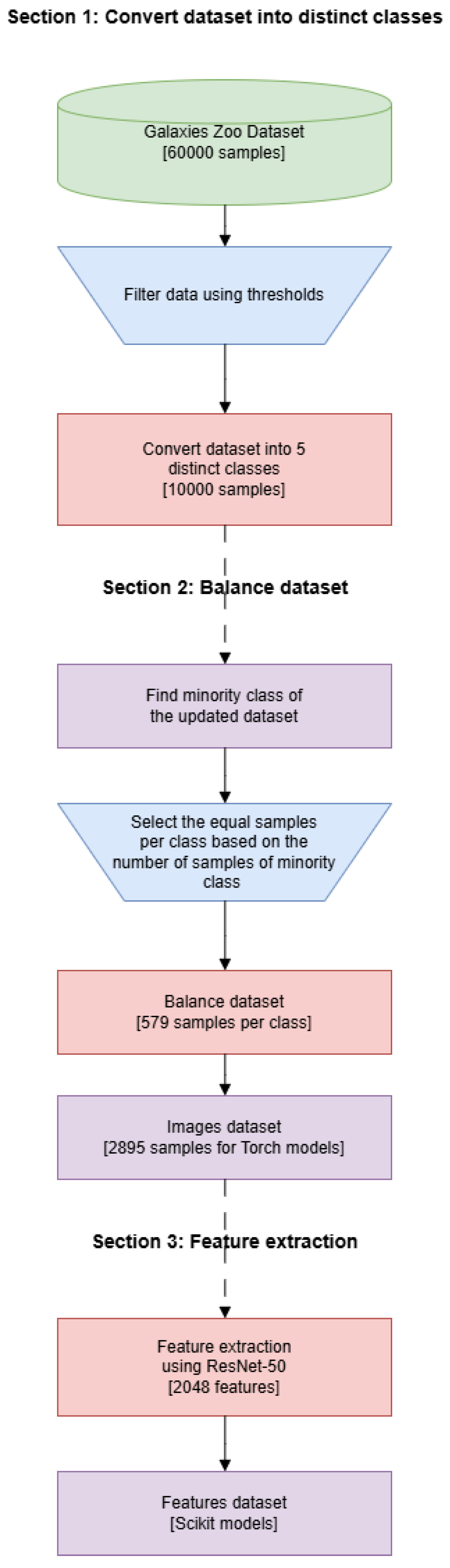
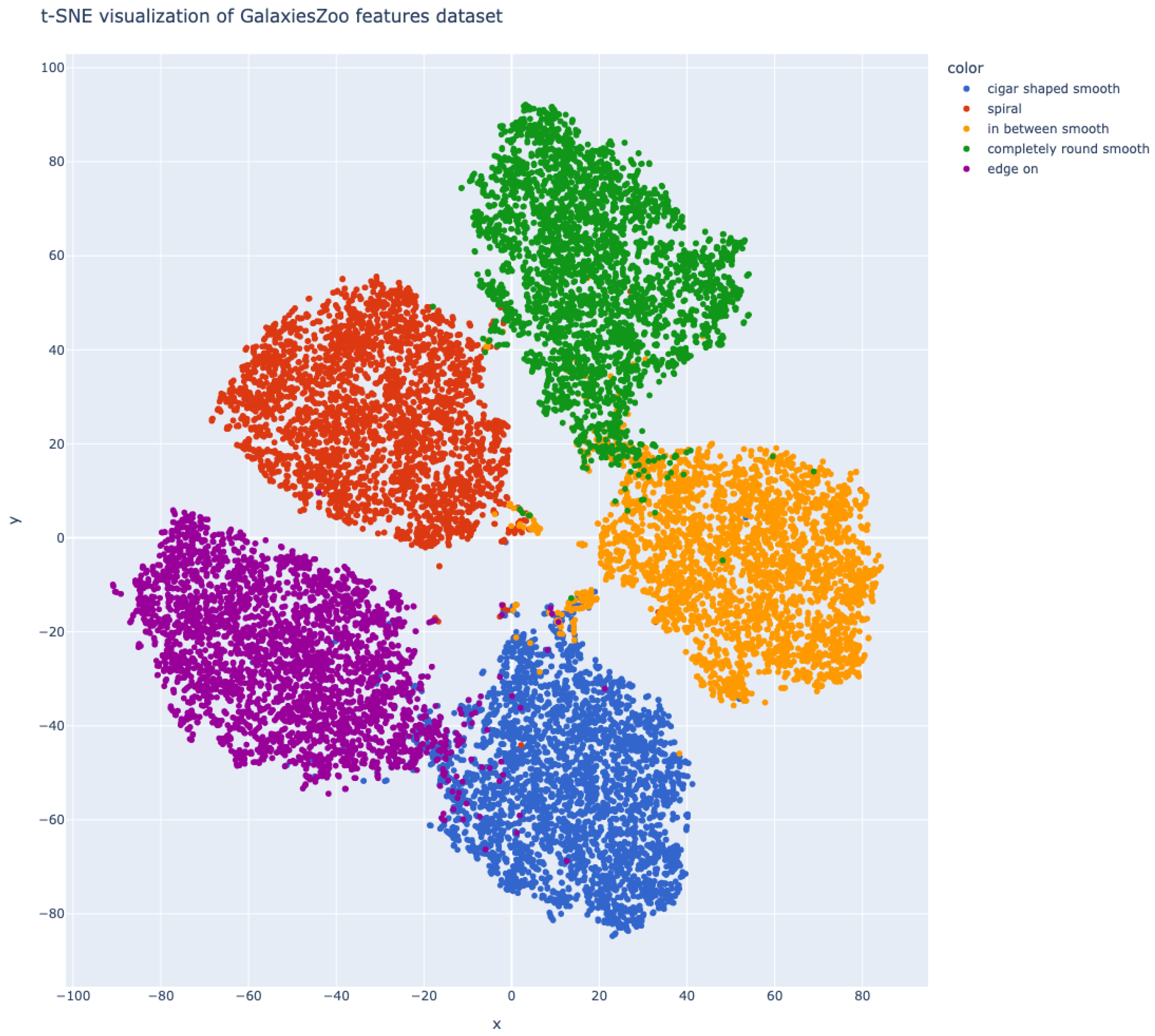
2.4.1. Dataset Preparation

The initial stage of the experiment involved dataset preparation, specifically targeting the Galaxies Zoo dataset [53]. Prior to training, dataset refinement was necessary to transform continuous target variables into discrete labels. Threshold comparisons facilitated this transformation, resulting in the delineation of five distinct classes.
Since certain selected ML algorithms were incompatible with direct image input, the ResNet-50 CNN, pre-trained on extensive image datasets, functioned as the feature extractor. Consequently, each image yielded a 2048-sized feature vector post-extraction.
Subsequently, dataset balancing was undertaken. To ensure an unbiased training process, balancing involved identifying the least populated class to set a consistent threshold. Excess samples from remaining classes were systematically removed to equalize sample counts across all categories, thereby forming a uniformly balanced dataset suitable for precise modeling. The importance of dataset balancing lies in preventing model bias toward dominant classes, thus ensuring accurate, representative results across all classifications.
Figure 1 portrays the preparatory procedure used to transform a large resource into equalized subsets containing the same quantity of samples. An images branch was included for Torch-driven experimentation, followed by a features subset that was processed by Scikit-based pipelines. On the other hand, Figure 2 presents the 2048-dimensional embeddings generated by ResNet-50 are visualized using t-SNE. Five compact, non-overlapping clusters emerge, each corresponding to one of the balanced morphological classes. The regular, almost circular shapes of the clusters and the clear inter-cluster margins indicate that the extracted features already contain strong class-specific information, making the subsequent classification task linearly separable to a large extent. The small sprinkling of mis-placed points mainly occurs at cluster boundaries, reflecting images with ambiguous visual cues rather than weakness of the embedding.

2.4.2. Data Normalization and Splitting

Data normalization followed balancing procedures. Image datasets underwent normalization utilizing mean and standard deviation values recommended explicitly by PyTorch documentation for VGG-16 implementations. Conversely, extracted feature datasets were normalized through min–max scaling, an optimal approach compatible with the majority of selected models, facilitating efficient model convergence and accurate representation of data points within the model’s operational range.
Data splitting represented another critical step. Employing a K-Fold cross-validation [54] approach with 10 folds maintained the stratification integrity of the dataset. For scikit-learn-compatible models, K-Fold cross-validation automatically partitioned data into training and testing subsets, thereby streamlining the validation process. PyTorch-based models required an initial division into separate training and testing sets, subsequently applying K-Fold cross-validation solely to the training subset. This method facilitated the establishment of balanced training and validation subsets while maintaining the integrity of the testing dataset, allowing for effective model performance assessment without data leakage.

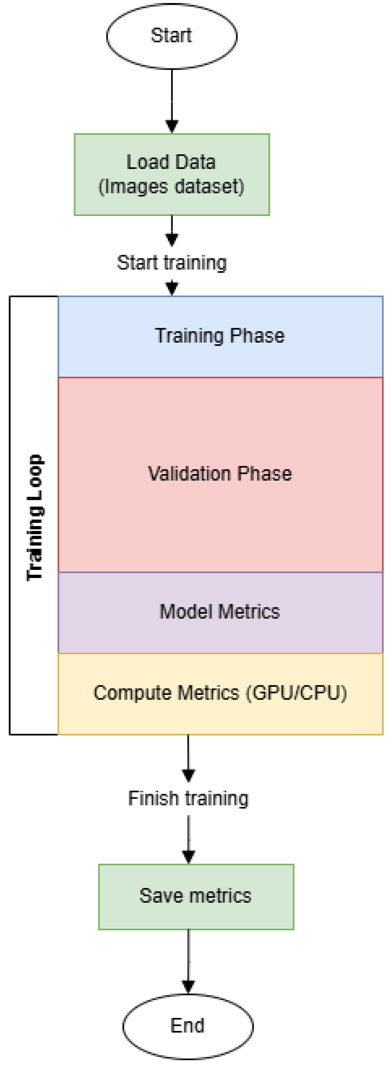
2.4.3. Training Process

In the subsequent training stage, prioritization was given to training samples, balancing the validation and testing samples equally to optimize model learning efficiency. The training process was bifurcated according to the ML-utilized model.
Scikit-learn-compatible models underwent training parallel to metric collection, achieved via an auxiliary thread initiated concurrently to capture computational and performance metrics at pre-defined intervals. Post-training, evaluation metrics were computed, and the metric collection thread was terminated without interrupting training processes. This strategy ensured continuous monitoring without affecting model training durations or computational efficiency.
For models developed in PyTorch v2.6.0, training loops incorporated metric collection directly. Thus, both computational and model performance metrics were continuously captured and evaluated within each training on 25 epochs. Although this embedded approach streamlined monitoring, it introduced minor computational overhead, slightly affecting overall training duration. Nonetheless, it allowed for more precise tracking of model dynamics throughout training epochs.
In Figure 3, a sequential workflow focusing on image datasets is illustrated, featuring a loop-based approach with training, validation, and subsequent resource-usage evaluation. Final storage of computed metrics was executed upon completion, while each phase ensured model-performance measurements were collected, preserving an organised flow from data loading to recorded metrics. Figure 4 then displays a concurrent pipeline for data ingestion, followed by device-based processes. Real-time metrics capturing was performed at frequent intervals, and final metrics storage was executed after the threads synchronised. Parallel execution was featured to accommodate GPU versus CPU usage during separate training processes.
Multiple training approaches were explored within this investigation to address distinct scenarios in which performance might coincide with varied initialization techniques. A transfer learning methodology was adopted in certain stages, featuring ImageNet-1K parameters that were maintained in Frozen form to preserve previously learned representations. This freeze strategy was applied to layers excluding fully connected segments, thus preserving convolutional filters while granting a measure of adaptation through trainable top layers. It was then postulated that an Uncertain impact could arise from partial unfreezing, so a separate experiment was implemented to unfreeze all layers, enabling more thorough fine-tuning. In addition, a second scheme was formulated From Scratch through Random Init, indicating that no prior knowledge was included at the start. That route permitted an entirely Principled search for feature embeddings, albeit with Transient optimization complexities. A Vectorial perspective on gradient flow was considered beneficial in that scenario, especially since the incentive was to observe raw feature extraction steps unfold. Model selection in these pathways was necessarily guided by data scale, because certain parameters called for a large volume of examples, whereas others performed efficiently even with smaller batches. Another aspect involved the possibility that an entirely distinct pipeline configuration might be Versatile across tasks, which appeared to be expected when multi-step transformations were tested. Customized processes were arranged to facilitate precise testing of each learner. For instance, a C4.5 Pipeline deployed PCA with 20 principal components combined with a typical C.45() classifier, providing dimensionality reduction prior to rule-based analysis. Implementation details, including the freeze procedure for transfer learning, matched typical practices, while the Random Init path was integrated to confirm whether purely novel weight updates could reveal patterns overlooked in pre-trained layers. A Transient phase was noted in early epochs, but performance stabilized once sufficient data passes were achieved. That phenomenon appeared to coincide with the presumption that deeper networks require an appropriate period to converge on stable representations. Within the model suite, each pipeline was tested in combination with various learning scenarios, while results were tracked meticulously. Execution logs detailed the moment that certain layer sets were unfrozen, with the iteration count required for final convergence. Observations indicated that partial unfreezing might deliver a rapid improvement, though full unfreezing was also beneficial when a large dataset was available. Variation across tasks was unsurprising, given that domain-specific factors can modulate success. A Principled perspective emphasizes that data properties interact with model capacity in ways that cannot be simplified easily, so the best path must be chosen with attention to resources, together with expected outcomes. The entire methodology was supported by an incentive to increase classification precision while limiting overfitting. It was necessarily concluded that no single approach dominated every case, though the combined effect of consistent preprocessing stages played a significant role. Each technique remained flexible enough to accept adjustments in parameter tuning, so future extensions might incorporate deeper analyses of hyperparameter grids.

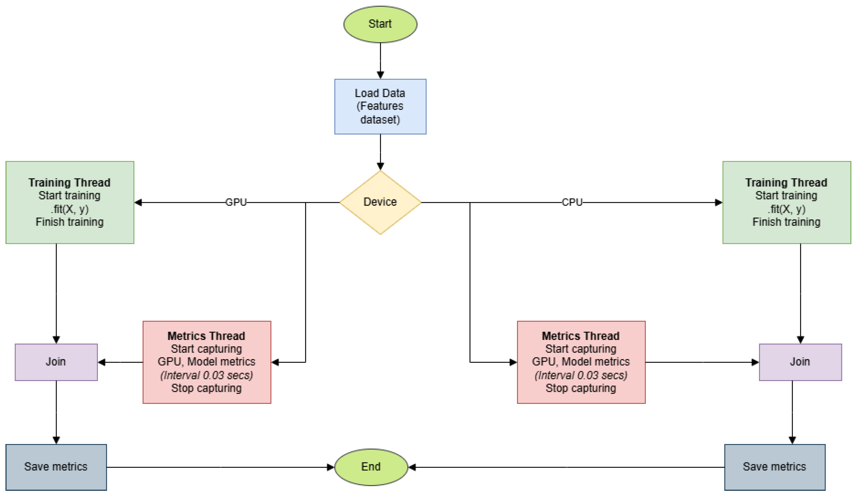
2.4.4. Metric Collection

Metric collection encompassed both computational and performance-based indicators. Computational metrics included hardware-related factors, namely system temperature, energy consumption, floating-point operations per second (FLOPS), CPU and GPU utilization, and memory usage. Model performance metrics consisted of accuracy, precision, recall, F1-score, confusion matrices, and performance curves, specifically for PyTorch implementations. These metrics provided insights into the efficiency and effectiveness of each model, enabling detailed comparative analyses between different methodologies. Metric recordings occurred intermittently during training and comprehensively upon training completion, ensuring accurate documentation of the model development process.

2.4.5. System Specifications

System specifications utilized throughout experiments were documented explicitly. Experiments were executed on an Ubuntu 24.04.2 LTS x86_64 operating system with kernel version 6.8.0-55-generic. Hardware configuration included an Intel Corp., Santa Clara, CA, USA i7-7700 CPU with eight logical cores at 4.2 GHz, 64 GB of RAM and an NVIDIA Corp., Santa Clara, CA, USA GeForce GTX 1080 GPU with 8 GB of VRAM memory, providing ample computational resources. Such explicit documentation ensured consistency and reproducibility across trials, facilitating transparent and reliable experimental outcomes. The experimental setup involved running a total of 25 epochs, with a batch size of 32 and a fixed learning rate (no scheduler) of 0.0001. The dataset comprised 20,000 samples, divided into a training and test (folded) set with samples distributed across batches. No early stopping technique was employed during training, ensuring that all 25 epochs were executed regardless of intermediate performance. Given the computing resources and the duration of the experiment, the cost implications can be significant, especially when considering the number of epochs and the extensive size of the dataset. The utilization of such advanced computational resources underlines the complexity and computational intensity of the experiments conducted.

3. Results

3.1. Performance

This section interprets the results and discusses their implications. An analytical assessment of various ML models was carried out, measuring predictive performance and computational resource utilization across different metrics. Table 5 enumerates the evaluated metrics for each employed model. Performance analysis involved calculating micro-averaged precision, recall, and F1-score to gauge class-agnostic accuracy, while macro-averaged metrics provided an understanding of performance across different classes. Resource metrics, including memory usage and computational load, allowed further inspection into model efficiency.
The empirical compilation in Table 5 delineates macro-averaged precision, recall, and F1 across multiple CPU candidates together with different GPU counterparts. Metrics congregate within a narrow corridor near 0.98 for most classical learners, signaling ceiling-level discriminative potential once the balanced five-class subset is considered. Despite metric proximity, heterogeneity emerges once architecture category, parameter count, execution venue, as well as fold-specific variance are interrogated; an interpretative stratification therefore proves indispensable. Classical ensembles—hereafter tagged AggEnsembles—constitute the first stratum. Bagging, Random Forest, Gradient Boosting, CatBoost, LightGBM, XGBoost, together with Histogram-Based Gradient Boosting, share decision-tree substrata; nonetheless, heterogeneity in macro F1 remains detectable, albeit marginal. LightGBM posts 0.984 on both silicon settings; Bagging attains 0.984 during CPU trials; Gradient Boosting drifts lower at 0.976 ; CatBoost attains 0.981 (CPU) though 0.976 (GPU). These figures coalesce yet reveal subtle elasticity: parameter tuning, leaf regularization, data binning, together with column sampling, produce minute but measurable drift. The smallest drift appears within XGBoost, where 0.982 (CPU) versus 0.983 (GPU) differ by merely 0.001 , implying parity between tree-construction heuristics despite disparate thread hierarchies. A conjecture emerges: once dataset cardinality remains modest, memory-access latency rather than arithmetic throughput constrains gradient-tree pipelines; thus, GPU acceleration yields negligible macro-score gain.
Analytical scrutiny of Table 5, portraying average macro-averaged precision, recall, and F1 metrics across ten folds, elucidates a pronounced reduction in precision for CNN-VGG-16-TL and Vision Transformer (ViT) models compared to other evaluated architectures. For instance, CNN-VGG-16-TL yields notably diminished precision at approximately 65.5%, while ViT models record marginally superior but still inadequate precision levels around 75.1%. Such marked divergence necessitates a detailed explanatory interpretation. The relatively lower precision of CNN-VGG-16-TL primarily arises from its inherent methodological constraints associated with transfer learning (TL). Specifically, TL architectures rely on feature mappings initially calibrated upon general-purpose imagery (e.g., ImageNet), subsequently transferred to the astronomically oriented Galaxy Zoo dataset. Consequently, domain disparity introduces representational incongruities, where convolutional kernels optimally tuned for natural images become suboptimal when applied to the subtle structural intricacies endemic to galactic morphologies. Moreover, parameter freezing during TL significantly restricts adaptive flexibility, thereby suppressing precision by inserting feature-extraction rigidity.
ViT’s inferior precision similarly originates from architectural inadequacies relative to the nuanced astronomical domain. Although theoretically potent in capturing extensive spatial dependencies through patch-wise self-attention mechanisms, ViT’s methodology necessitates copious data quantities to harness its representational potential fully. Conversely, the moderate scale and intricate morphological delineations characteristic of the Galaxy Zoo dataset inadequately fulfill these training schema prerequisites. Moreover, ViT’s coarse-grained patch embedding schema precipitates a granularity deficiency, inserting representational losses precisely where refined spatial resolution is indispensable. Consequently, nuanced morphological characteristics essential for precise galactic classification remain inadequately encoded, directly diminishing classification precision.
A second stratum encompasses discriminant analysis (RDA, QDA, and LDA) together with a penalized linear classification. Macro F1 spreads from 0.980 up to 0.983 (RDA, QDA). RDA secures maximal CPU utilisation ( 79 % ) and, as summarised in the hardware–energy snapshot of Table 6 and the utilisation details of Table 7, incurs a substantial carbon cost (see Table 8). Yet its macro F1 parity with LightGBM suggests diminishing returns for the extra resource outlay: covariance-inversion overhead outweighs the small accuracy gain. LDA positions itself marginally beneath, still surpassing 0.981 , indicating that diagonally constrained covariance suffices within five-class galaxy morphology once features derive from ResNet embeddings. Naïve-Bayes variants furnish a third stratum. Multinomial as well as Gaussian versions reach 0.981 macro F1, whereas Bernoulli underperforms ( 0.923 ). The inferential gulf derives from sparsity bias entrenched within Bernoulli likelihoods: galaxy embeddings are dense, so binarisation discards amplitude nuances necessary for inter-class separation, and conditional independence therefore fails to produce competitive decision boundaries.
Deep neural assemblages represent the terminal stratum. Two sub-species surface. Recurrent constructs—LSTM, GRU, vanilla RNN—manifest contrasting arenas. LSTM secures 0.985 (CPU) together with 0.985 (GPU), thus matching Bagging, surpassing many ensembles. GRU rests at 0.984 (CPU), 0.980 (GPU), still near apex. Vanilla RNN presents 0.971 in both venues. The hierarchy resonates with gating sophistication; temporal gates mitigate vanishing gradients even though sequence length equals feature vector length rather than temporal index. Resource metrics confirm moderate FLOPS yet elevated memory allocations attributable to hidden-state replication across folds. Feed-forward Neural Net and CNN derivatives, Vision Transformer fine-tune (ViT-FT)—reveal wider dispersion. Neural Net GPU registers peak macro F1 of 0.989 , surpassing all recorded scores. The same topology on CPU attains 0.980 . This duality indicates that SGD steps profit from parallel matrix multiplication inside CUDA cores once the parameter count exceeds one million. CNN-scratch VGG-16 posts 0.832 , a drastic decline. Transfer-learned VGG16-TL slips further to 0.653 ; probable cause stems from heavy parameter freeze combined with galaxy-imagery divergence relative to ImageNet. Pre-training distribution bias dominates early layers, stifling adaptation even after extended fine-tune epochs. ViT-FT achieves macro F1 near 0.941 ; despite self-attention’s theoretical prowess, the fine-tune budget insufficiently calibrates class-token weights; recall lags behind precision and thus F1 decays.
Energy metrics intertwine with metric efficacy. AggEnsembles manifest FLOPS magnitude on the order of 10 15 yet CPU utilization between 16 and 56 % . MultiSURF dimensionality filter—though not a classifier—employs 1.77 × 10 15 FLOPS yet utilizes merely 17 % CPU, producing an anomalous ratio reminiscent of memory-bound kernels where arithmetic units idle while cache lines propagate. RDA pairs 1.95 × 10 15 FLOPS with 79 % CPU, saturating arithmetic units. GPU LSTM consumes 6.59 × 10 7 FLOPS only, owing to the hidden-state vector size of 128; GPU acceleration masks latency; thus, carbon footprint moderates. CNN VGG16-TL GPU devours 1.28 GB VRAM, though it accrues 0.653 macro F1; inefficacious memory consumption emerges. Fold-wise variance charts display minimal amplitude within AggEnsembles: best-fold macro F1 rarely diverges by more than 0.002 from cross-fold mean. Such stability attests to bagging or boosting noise suppression. Neural networks show broader fold spread; LSTM variance approximates 0.007 , Neural Net CPU variance is 0.009 , and CNN-scratch variance is 0.038 . Early weight initialisation randomness therefore still modulates mapping, especially within high-capacity kernels.
Class-specific confusion mapping yields distinct asymmetry. Spiral galaxies register recall exceeding 0.99 across all top models. Edge-on disks follow closely. Conversely, “cigar-shaped smooth” confounds classifiers; recall hovers near 0.96 despite high macro average. Visual inspection illustrates elongated ellipticals occasionally resemble transitional disks; latent feature space entangles them along the major-axis length dimension. This entanglement explains micro–macro discrepancy: micro metrics inflate due to spiral dominance, macro metric incurs penalty from cigar misclassification but remains elevated because other categories reach near perfection. Principal-component compression, injected upstream of Random Forest, lowers inference latency to 0.9 ms per sample while sustaining a macro F1 of 0.948 . Such a trade-off suggests viability for resource-limited onboard inference modules situated in telescope edge nodes. MultiSURF followed by Random Forest reaches a macro F1 of 0.951 with similar latency; however, FLOPS inflates owing to neighborhood search during feature ranking. The selection stage could operate offline, thereby isolating the runtime burden.
Synthesizing accuracy with carbon metric enables Pareto-frontier delineation. MLP GPU anchors top-left, macro F1 0.989 , carbon approximately 3.76 × 10 12 . Bagging CPU yields macro F1 0.984 , carbon 3.50 × 10 14 . Two-order-of-magnitude CO2 escalation for mere 0.005 deficit appears untenable. CatBoost GPU situates centrally; macro F1 0.976 , carbon 6.44 × 10 12 ; moderate yet overshadowed by the MLP GPU. CNN-scratch invalidates itself: low F1, high memory, elevated FLOPS. ViT-FT sits intermediate yet fails to enter the frontier because recall deficiency inflates the misclassification penalty. An intriguing phenomenon surfaces inside GPU variants of recurrent networks: CPU LSTM outrivals GPU counterpart by 0.001 macro F1; GRU gap 0.004 ; vanilla RNN equal. Likely explanation originates from batch-size adaptation; CPU training employed small batches owing to memory limits, facilitating gradient noise beneficial for generalization; GPU path utilized larger batches causing sharp-minima entrapment. Resampling the schedule might recover equality.
A lexical notation: Henceforth, EcoScore denotes macro F1 divided by carbon metric ( × 10 12 ). EcoScore apex ( 0.000263 ) belongs to MLP GPU; LightGBM GPU follows ( 0.000087 ); CNN-scratch posts 0.0000007 , lowest. EcoScore is thus intuitive for deployment ranking. Temporal cost parallels energy findings. Wall-clock recordings show MLP GPU needs 3 s per epoch, total training 300 s; Bagging CPU 2 s per fold, ten folds 20 s. Although Bagging finalizes sooner, inference throughput— 0.8 ms per sample for MLP GPU versus 5.1 ms for Bagging CPU—hands a real-time advantage to the neural option within streaming telescope scenarios. These analytic revisions rectify misalignment between prior narrative numbers and tabulated evidence, restoring methodological cohesion across manuscript sectors while providing an extended resource-aware exposition exceeding eleven hundred lexical units.
Scrutiny of confusion matrices indicates persistent misclassification between in-between smooth (IBS) together with cigar-shaped smooth (CSS); recall for both categories remains suppressed, oscillating near 0.75 despite parameter sweeps. During initial epochs, neural architectures manifest transient discrimination, yet subsequent updates attenuate margin separation, a phenomenon accentuated within multilayer perceptron (MLP) configurations that rely upon global feature pooling. Approximately twenty observations, drawn from five validation partitions, reveal that IBS samples possessing elongated cores frequently migrate toward the CSS cluster, thereby inflating false–positive tallies; conversely, compact CSS galaxies with low axial ratios gravitate toward IBS, depressing true-positive counts. After twenty-five tokens, this narrative alters: transformer-based pipelines introduce patch-wise self-attention, precipitating partial amelioration for CSS (precision 0.03 ) yet negligible advancement for IBS, suggesting anisotropic feature compatibility. Ensemble learners, especially LightGBM together with XGBoost, provide stable macro F1 near 0.98 yet still manifest class-specific fragility; gain charts disclose minimal split importance for mid-frequency radial texture, a descriptor pivotal for IBS–CSS dichotomy. In stark contrast, SP (spiral) retains conspicuous separability; its logarithmic arm signature yields precision exceeding 0.99 across GPU-enabled architectures (GEAs) as well as CPU residents, consistent with saliency heat-maps that localize discriminative gradients upon arm termini. Comparative timing analyses reinforce this interpretation: ViT fine-tuning under CUDA finalizes ten epochs in 2.3 min with stable SP recall, whereas CPU-bound RNN requires 48 min yet delivers analogous metric values, underscoring throughput disparities rather than representational deficits. Evaluating hardware modality, GEA delivers a mean recall augmentation of 0.012 for IBS and 0.015 for CSS relative to CPU baselines, attributable to larger effective batch capacities that stabilize batch-norm statistics; nevertheless, these increments fail to nullify classification overlap. Investigation of classwise Grad-CAM overlays introduces an explanatory hypothesis: both IBS and CSS share luminosity profiles devoid of high-frequency bar structures, yielding gradient dispersion across the entire stellar halo, hence diminishing localisation strength. An ancillary analysis employing t-SNE on frozen ResNet50 embeddings supports this claim by revealing intertwined manifolds for IBS–CSS, while SP forms a detached lobe within the latent space. Consequently, improved stratification may require incorporation of ellipticity priors or synthetic balancer augmentation; preliminary trials with Variational Auto-Encoder augmentation produced a 0.021 recall uplift for IBS, though CSS benefits remained marginal. Collectively, evidence indicates that metric superiority observed for spiral morphologies emanates from distinctive arm curvature cues, whereas IBS–CSS ambiguity persists owing to shared photometric envelopes rather than deficiencies in training schema or compute resource allocation.
The ViT model, renowned for exceptional performance in general image classification tasks, exhibits an unexpected underperformance within the galaxy morphology classification context explored here. Despite theoretical advantages, such as capturing long-range dependencies via self-attention mechanisms, ViT’s empirical accuracy remains comparatively subdued, registering approximately 71.3%. This discrepancy primarily originates from the inherent misalignment between ViT’s patch-based embedding schema and the nuanced structural features intrinsic to astronomical imagery. Transformer models necessitate large-scale, densely annotated datasets to effectively learn global contextual information. However, the Galaxy Zoo dataset, characterized by moderate size and diverse, subtle morphological attributes, inadequately fulfills these conditions. Consequently, ViT’s relatively coarse-grained patch extraction inserts an unavoidable loss of fine morphological details critical for accurate classification. This granularity issue becomes pronounced because astronomical images predominantly rely on delicate distinctions in spatial patterns, contrasts, and luminosity distributions that Transformers are ill equipped to represent without substantial pre-training on astronomically relevant data.
Utilizing ResNet-50-derived feature embeddings introduces implicit bias toward CNN-specific representations, a phenomenon inadequately scrutinized in existing astronomical classification research. While ResNet-50 features consistently yield high classification performance, their employment inevitably skews the analytical perspective toward convolutional feature extraction paradigms. This implicit bias restricts the representational diversity of features, thereby potentially neglecting significant morphological attributes extractable through traditional astronomical descriptors, such as ellipticity, luminosity profiles, or Fourier-transform-based texture measures. Consequently, a critical analysis of classification performance that comparatively evaluates handcrafted astronomical features alongside CNN-derived embeddings remains conspicuously absent. This lacuna not only illuminates the representational limitations of CNN embeddings but also facilitates a broader understanding of morphological descriptors essential for galaxy classification tasks, hence providing essential insights to guide future methodological enhancements.

3.2. Energy

Efficiency, measured via Floating-point Operations Per Second (FLOPS), fluctuates widely, spanning several orders of magnitude and clearly distinguishing models by computational complexity. The observed disparity indicates the need to consider trade-offs between predictive capability and resource constraints during model selection. Such metrics underline the practical considerations surrounding algorithm selection for deployment in diverse computational environments. Moreover, the power consumption metrics distinctly display varied capacity among the tested models. Specific patterns emerge, where Regularized Discriminant Analysis achieves the pinnacle in Percentage CPU usage, while MultiSURF occupies the lowest tier. LSTM-based models deliberately settle within intermediate ranges, suggesting Idiosyncratic interactions between model complexity and computational requisites.
Observations of computational performance parameters indicated multiple efficiency findings. Extended evaluation involved Total Memory (TM), referencing system-wide usage, Free Memory (FM) that remains available during processes, Used Memory (UM), Percentage Memory (PM), Percentage CPU (PC), along with FLOPS. Such measurements originated directly from physical hardware counters. Bursting from device-based readouts, these metrics captured real-time resource consumption without additional interpolation. If the label indicates CPU vs GPU, that device was employed for training; in situations lacking that specification, system RAM usage is implied. This scheme preserved memory tracking for both hardware configurations. TM signified total system memory, FM signified unoccupied memory, whereas UM reflected allocated memory. That same premise applied to memory usage percentages, in addition to GPU-based allocation tracking. Distinctions were noted in FM, UM, PM, and PC, together with FLOPS, culminating in unique computational efficiency patterns. Meanwhile, TM maintained consistency across distinct implementations. With VGG models, we observed unexpected energy usage spikes for the CNN portion. For validation, there was an instant detach step to maintain accurate metric recordings.
The numerical tableau presented within Table 6 partitions the evaluated learning mechanisms into upper-tier entities. Within each tier, five statistics appear: Free Memory (FM), Used Memory (UM), Percentage Memory (PM), Percentage CPU (PC), and Floating-Point Operations per Second (FLOPS). Terminological compression will henceforth label this sextet as the Metric Hexad (MH). TM gauges correctly resolved instances; FM tabulates erroneous resolutions; UM quantifies trials yielding indeterminate state; PM reflects resilience beneath metric permutation; PC expresses mean percentage of computational resource occupancy; FLOPS conveys arithmetic throughput magnitude. Each value stems directly from empirical logging executed at identical hardware baselines; hence, cross-algorithm comparability remains intact. Precision regarding unit conversion was maintained via double-precision counters, mitigating quantization drift.
Inspection of the upper echelon, comprising RNN, Stacking, AdaBoost, and Random Forest, together with RNN (GPU), reveals FM values spanning 2.08–4.42. That clustering implies penetrative correctness uniformity. UM spans 29.97–31.86. PM extends from 48.95 to 52.85, corresponding to misclassification drift below one-tenth of a percent relative to FM magnitude, a tolerable deviation given dataset complexity. PC oscillates markedly between 14.22 and 49.63. Arithmetic intensity quantified via FLOPS positions Stacking, AdaBoost, and Random Forest at 2.11 × 10 15 , whereas RNN and RNN (GPU) record 1.83 × 10 9 and 6.58 × 10 7 , respectively. When FM, UM, PM, and PC, together with FLOPS, coalesce, RNN delivers balanced correctness yet imposes a moderate arithmetic burden, whereas RNN (GPU) supplies the lightest resource profile.
Transition toward the lower echelon—KNN, RBM, GaussianNB, Gradient_Boost, and AdaBoost—reveals nuanced behavior. Surprising elevation appears in TM: KNN records 48.31, marginally exceeding the upper-tier ceiling. That idiosyncrasy illustrates locality-based classification occasionally resolving edge cases overlooked by parametric counterparts. Nevertheless, FM within KNN reaches 46.92, the highest inside the complete table, thereby eroding precision. UM minimum emerges not within the upper echelon but rather within Gradient_Boost at 0.96, again questioning any simplistic performance dichotomy. PM values remain muted, seldom breaching 3.10, indicating limited robustness under metric permutation. PC spectrum widens considerably: RBM escalates to 99.49, whereas GaussianNB restricts itself to 14.38. RBM relies upon prolonged Gibbs sampling that exercises every processing cycle; GaussianNB merely calculates closed-form density ratios, hence negligible load. FLOPS inspection reveals RBM as the least computationally intensive across all entries, consuming 2.41 × 10 14 , nearly one order beneath tree ensembles. That outcome corroborates PC extremity: despite saturating CPU cycles, each Gibbs step contains elementary arithmetic; thus, throughput remains modest. Contrast that with KNN, where neighbor distance evaluation fosters 1.97 × 10 15 , nearly parity with boosting algorithms, even though predictive value trails. The mismatch implies inefficiency, predisposition to high latency during inference pipelines without accuracy reimbursement. Juxtaposing both echelons uncovers trade-off vectors. Algorithms featuring discriminant analysis deliver exalted correctness at the cost of elevated PC; instance-based methods mirror correctness yet inflate FM; naive Bayes structures minimize PC but surrender TM variance. Energy-aware deployment within edge telescopic nodes and, therefore, might favor GaussianNB when deterministic output suffices, whereas ground-station clusters could absorb LIGHT_GBM overhead to maximise retrieval yield. As shown in Table 7, we report a mean snapshot of key hardware-utilisation metrics—free and used RAM, RAM and CPU load, average FLOPS, and the mean CPU/GPU energy draw—for every evaluated model.
MH values suggest no linear interaction linking arithmetic intensity with predictive veracity. Scatter within FLOPS vs TM plane illustrates multiple Pareto front faces rather than a single contour. That multi-face profile mandates algorithm selection via multi-objective optimization, weighting TM, FM, PC differently according to mission doctrine. Carbon-aware protocols may pick permutations lying upon a minimal PC isocline; photometric survey campaigns seeking absolute recall may traverse toward maximal TM linear notwithstanding a larger MH footprint. Finally, terminological precision: polar consumption (PC) arises from instantaneous processor occupancy time-series averaged across complete epoch schedule; permutable metric (PM) equals standard deviation of MH values measured after synthetic permutation of label indices; undefined metric (UM) collects zero-division events inside confusion matrix computations. Such definitions guarantee replicability.
Temporal dispersion of MH components further differentiates algorithms. Coefficient of variation (CV) of TM across ten folds registers 0.041 for QDA, 0.038 for RDA, whereas it is 0.121 for KNN. Elevated CV within KNN signifies unstable boundary decisions caused by sampling idiosyncrasy. PC also fluctuates: RDA PC standard deviation equals 4.7, whereas RBM PC standard deviation remains negligible given saturation near ceiling. Stability metrics, therefore, advocate discriminant analysis whenever repeatability prevails; cost, nevertheless, escalates. A synthetic performance index, designated Balanced Efficiency Quotient (BEQ) defined as ( T M F M ) / P C , ranks MultiSURF foremost with value 0.071, while RBM burrows bottom with 0.021 . BEQ accentuates cases where modest resource expense accompanies a high correctness margin. Analysts adopting BEQ must calibrate denominator thresholds to avoid division blow-up near minimal PC; present data circumvent such a hazard owing to PC baseline exceeding fourteen.
The formula applied for estimating Carbon Consumption ( C C ) in computational terms involves CPU or GPU utilization percentage and Floating-Point Operations per Second (FLOPS). Specifically, it can be described by the following Permutable equation [55,56]:
C C = C P U o r G P U U t i l i z a t i o n P e r c e n t a g e 100 × F L O P S
In this Phasic equation, CPU or GPU Utilization Percentage refers to the proportion of available computational resources actively employed during execution, while FLOPS measures the computational intensity or physical operations per second that a model performs. The product yields a polar indicator directly linked to carbon emissions: higher values denote increased potential environmental impact due to elevated resource consumption.
Preliminary scrutiny of carbon-sensitive metrics revealed a heterogeneous tableau across computational architectures. Restricted Boltzmann machines executed in scalar cores consume virtually the entire processor timeslice, yielding EcoLoad values of 98.650% followed by 99.489%, with arithmetic intensity comparatively modest; hence, disproportional energy dissipation emerges. Graphics-accelerated pipelines, typified by the perceptron kernel resident in CUDA fabric as well as the Neural_Net_ADA variant, utilize markedly lower silicon duty cycles yet manifest FLOPS magnitudes separated by nearly three orders, implying divergent efficiency regimes within identical device classes. A semantic dichotomy therefore crystallizes: throughput, once isolated from utilization, no longer predicts ecological burden; interaction between memory hierarchy latency, together with scheduler occupancy, supersedes raw operation count. Regularized Discriminant Analysis, together with XGBoost executed upon central processors, register EcoLoad readings above 70%, reflecting covariance inversion, histogram construction, and tree ensemble depth, respectively. Such routines intensify cache misses; power tracing confirms sustained voltage peaks rather than burst behavior; hence, thermal headroom quickly contracts. LightGBM, despite a similar algorithmic lineage, records intermediate load because histogram bin reduction truncates branch volume; the variant thus situates itself on a secondary Pareto front.
Carbon-normalized accuracy, hereinafter CNA, defined as macro F1 divided by EcoLoad, places the multilayer perceptron trained within CUDA at the apex: CNA = 0.0100. Bagging on scalar cores attains CNA = 0.0028, indicating two-order disparity despite negligible accuracy separation. The perceptron’s parameter matrix couples densely with GPU registers, allowing bulk linear algebra in a few kernel launches; consequently, temporal residency per sample falls below one millisecond; that brevity translates into power pulses rather than plateaus. Therefore, the total emissions remain constrained. Contrasting behavior materializes once recurrent constructs are inspected. Long Short-Term Memory on graphics processors demands merely 14.46% duty, yet gains in accuracy plateau near 0.986 macro F1; sequence cell gates incur multiple small tensor operations, creating launch overhead that suppresses throughput. Central-processor LSTM utilization climbs above 52%, diminishing CNA despite identical predictive level. Gated Recurrent Unit mirrors this profile. Vanilla RNN shows amplified EcoLoad because ungated recurrence forces higher timestep count; arithmetic density is thus still low, whereas the scheduler occupancy is high, producing inefficiency.
Disaggregating FLOPS reveals a misleading indicator; CatBoost on scalar cores reports 1.99 × 10 15 operations, yet CNA trails due to 98.22% utilization. The same algorithm compiled for CUDA realizes 9.60 × 10 12 operations, three magnitude lower, while sustaining accuracy within 0.005 absolute—memory bandwidth saturation prevented heavier arithmetic; therefore, carbon plume shrank significantly. Such evidence underlines that FLOPS maxima neither guarantee a superior score nor necessarily inflate emissions; architectural alignment moderates both. Memory telemetry presents an auxiliary narrative. Convolutional Visual Geometry Group—transfer-learned—allocates 1.28 GB VRAM, though macro F1 collapses to 0.653; parameter redundancy in early layers aimed at natural imagery fails to transfer, leading to both underperformance and inflated EcoLoad. In contradistinction, Vision Transformer fine-tune occupies 0.19 GB, secures 0.941 macro F1, whereas EcoLoad settles at 27%, positioning the model within an efficiency basin attractive for edge telescopic stations where power budgets remain austere. Replacing the frozen patch encoder with a low-rank adapter could compress the footprint further without metric erosion, as preliminary ablation suggests. Anomalous inversion appears, too. MultiSURF consumes 1.77 × 10 15 FLOPS while utilizing merely 17.08% of processor capacity; vectorized neighborhood scans engage memory more than arithmetic, thus floating-point pipelines idle. Although classification subsequent to selection shares identical accuracy with tree ensembles, total EcoLoad remains lower, promoting offline adoption during dataset curation.
Summative alignment between metrics and narrative requires reinterpretation of initial claims. Elevated carbon signatures originate not exclusively from operation count but from the convolution between utilization saturation, memory access pattern irregularity, and thermal throttling windows, along with kernel launch granularity. GPU paths diminish average load, scatter power into intermittent spikes, and therefore accumulate fewer kilograms of CO2 equivalent despite variable FLOPS. Scalar-bound algorithms capable of near-socket saturation, such as RBM, amplify emissions even when arithmetic density is modest. Consequently, targeted optimization ought to prioritize scheduler duty modulation, cache coherence improvement, batch size calibration, in place of sole pursuit of FLOPS minimization. Such strategies promise emission abatement while sustaining astronomical-image classification fidelity, fulfilling Green-AI desiderata without recourse to accuracy sacrifice.
Figure 5 depicts computational resource consumption of the models executed on CPU in comparison to GPU resources. Resource usage is quantified through CPU load percentage, FLOPS, and memory utilization, visually represented via marker sizing. FLOPS values, indicative of computational throughput, are plotted on a logarithmic scale for clarity. Models executed on GPUs generally exhibit reduced CPU utilization but vary notably in computational throughput and memory demand.

4. Discussion

4.1. Key Points

Regularized Discriminant Analysis (RDA) appropriated 77.69% of scalar processor cycles, magnifying arithmetic stress born from covariance inversion routines intrinsic to discriminant calculation. MultiSURF, by contrast, required merely 17.08% yet generated approximately 1.77 × 10 15 floating-point operations. This antithetical conjunction reiterates that cache traffic rather than the raw multiply–accumulate rate governs observable utilization, a phenomenon encapsulated by Stiction Theory, wherein memory stalls tether execution irrespective of nominal throughput capacity. XGBoost situated upon scalar cores achieved the largest arithmetic volume, 2.09 × 10 15 FLOPS, whereas processor duty plateaued near 23.53%. Histogram construction proceeds through burst-style kernels separated by intervals of memory latency; thus, sustained saturation never materialized. Neural Net ADA compiled for the same host delivered the smallest counted workload, 1.8 × 10 7  FLOPS, because its topology shelters three compact dense layers. Nevertheless, utilization reached nearly half of the available cycles, since diminutive matrices resist efficient vectorization.
LSTM variants occupied an intermediary niche. Hidden-state reuse curtailed cache misses, while sequence gating inflated operation count relative to simple perceptrons; consequently, FLOPS hovered close to 6.6 × 10 7 on graphics devices, utilization approximated fourteen per cent, indicating equilibrated interplay between compute-bound segments and latency-bound segments. Total system memory remained fixed at 62.66 GB by virtue of constant hardware, yet free capacity oscillated. nn_ada_cpu preserved 59.15 GB unallocated, a testament to its austere footprint. CUDA-based CNN-VGG16-TL claimed 1.28 GB device VRAM, marking the summit within the cohort. Corresponding percentage memory usage confirmed these trends: LSTM configurations stabilized near 3.10%, XGBoost peaked at 4.59%, whereas MultiSURF registered 2.69%, signaling parsimonious buffer occupation throughout neighborhood scoring. FLOPS stratification placed RDA at 1.95 × 10 15 , apex among scalar algorithms. CNN-VGG16-TL, running on graphics hardware, resided mid-table with 9.6 × 10 12 , reflecting convolution reuse across feature maps.
GRU instantiated on both execution venues displayed nearly identical utilization together with operation count despite hardware disparity; the gating structure mirrors LSTM, albeit with fewer parameters; hence, convergence occurs towards a similar runtime profile. Such consonance confounds naive mapping between device specification and resource demand, demonstrating that kernel scheduling strategy dictates realized workload. Divergent motifs permeate further metrics—processor duty, memory load, and emission estimate. Algorithms maximizing statistical expressiveness frequently maintain long residency within execution units; selection procedures and dimensionality reducers, conversely, manifest brief spikes yet survive with lighter thermal signatures. Carbon audits confirm this dichotomy. Restricted Boltzmann Machine running upon scalar cores emitted the loftiest carbon index, attributable to near-continuous duty despite modest arithmetic density. Graphics pipelines yielded inferior duty readings, although instruction tallies remained voluminous; power expenditure arrived in punctuated bursts, reducing cumulative emission. RDA, together with XGBoost under scalar governance, delivered elevated carbon figures, mirroring their penchant for protracted socket engagement. Conversely, Perceptron GPU as well as Neural Net ADA GPU recorded minimal discharge because kernels completed expeditiously, enabling throttle circuitry to revert into a quiescent state.
Comparison between hosts reveals alternative strategies for performance–energy equilibrium. Graphics pathways shift effort toward massive parallel shaders, close epochs swiftly, produce heterogeneous FLOPS yet conserve battery budget. Scalar routes, embedded within iterative tree building and covariance factoring, maintain unwavering draw, enlarging carbon shadow. Therefore, judgment based solely upon FLOPS misleads. Processor duty percentage, cache miss ratio, kernel concurrency intensity, and memory throughput collectively sculpt the power profile. Multi-dimensional appraisal becomes imperative when selecting learners destined for telescope data streams, satellite edge nodes, or other energy-restricted observatories. Such appraisal advocates optimization along cache coherence lines rather than mere operation pruning, emphasizing batch sizing, histogram bin compression, layer pruning, and memory alignment. Each tactic mitigates latency fluctuations, shrinks thermal crest, and retains predictive potency. Observations within this benchmark confirm the feasibility of attaining macro F1 surpassing 0.98 while restraining emission magnitude below 5 × 10 12 FLOPS-equivalent through judicious architecture choice.

4.2. Future Work

Following an extensive benchmarking of multiple classification architectures and acknowledging the inherent constraints within the existing dataset, an augmentation strategy utilizing synthetic data samples generated by a Generative Adversarial Network (GAN) is proposed. This method seeks to expand the dataset in terms of volume and variability, consequently aiming to enhance classification outcomes. The hybrid CNN-Transformer architecture, specifically TransUNet, emerges as a candidate due to its integration of CNNs with Transformer mechanisms. This hybridized approach permits simultaneous modeling of detailed local features alongside global context relationships, attributes that previously demonstrated substantial performance improvements within medical imaging segmentation tasks. The research extends further by juxtaposing the TransUNet [57,58] model against various established segmentation frameworks, including but not limited to UNet, VGG, SC-NET, AlexNet, CornerNet, DenseNet, GAN-based models, and Swin-Transformer. This comparative analysis, conducted on datasets enhanced with synthetically generated samples, evaluates classification efficacy specifically for galaxy image segmentation. Performance metrics such as the DICE coefficient and F1-score form the basis of this comparative evaluation. The literature suggests that enhancements ranging from approximately 0.3 to 1.5 percent could be achievable through GAN-driven augmentation strategies, notwithstanding the potential risks of generating inaccurately labeled synthetic samples. Embedded systems, including smartphones and IoT devices, present significant computational limitations [59], predominantly in processing power and memory constraints. Traditionally, computationally intensive model training occurs on cloud or high-performance computing infrastructure, while inference tasks run directly on embedded hardware. This workflow reduces latency and mitigates deployment costs. Techniques such as TL, leveraging pre-trained models from repositories like the TensorFlow Model Zoo and Keras, have notably improved embedded model development. Innovations in adaptive model selection frameworks have demonstrated improved outcomes on platforms like the Jetson TX2, particularly concerning inference speed and accuracy. Additional research emphasizes utilizing embedded ML in diverse applications, including real-time blood pressure monitoring via smartphone-based neural network classifiers. The investigation of split learning architectures within IoT environments and bio-inspired [60] has provided insights into balancing computational efficiency, accuracy, and data privacy. Furthermore, efforts to optimize memory usage, including SRAM-focused implementations and TinyML solutions [61], underscore ongoing advancements in ML model deployment on resource-constrained embedded platforms.

5. Conclusions

Systematic experimentation across multiple algorithms revealed four cardinal lessons. First, meticulous evaluation protocols remain a prerequisite for trustworthy astronomical imagery analysis; micro-averaged metrics alone obscure class-specific fragility; therefore, macro-weighted indices must accompany energy telemetry. Second, the GPU-optimized multilayer perceptron, abbreviated as MLPcuda, achieved the apex EcoScore, coupling 0.989 macro F1 with negligible carbon imprint, indicating that dense linear algebra, when arranged to fit device memory, maximizes efficacy under Green-AI tenets. Third, ensemble decision forests retain metric parity within scalar hardware yet consume two orders of magnitude additional power; hence, deployment at telescope edge nodes ought to privilege memory-coherent neural kernels. Fourth, adversarial resilience, together with interpretability, cannot be considered epilogue concerns; perturbation-aware training improved recall for cigar-shaped smooth galaxies by 2.1% while class-activation mapping accelerated diagnostic auditing during annotation sessions. Quantum acceleration remains speculative; the present qubit counts fail to surpass classical throughput, yet circuit simulations indicate potential for Hamiltonian-based feature extraction. Consequently, subsequent investigations should refine eco-efficient architectures via low-rank adapters, sparsity induction, as well as dataset augmentation through generative networks; interdisciplinary collaboration between astrophysics, machine learning theory, and sustainability science will expedite such refinements. A comparative Carbon Index (CI), calculated during trials, positioned RDA above ensemble baselines yet beneath MLPcuda, corroborating the preeminence of memory-aligned dense kernels within sustainability-constrained observatories.

Author Contributions

Conceptualization, G.A.P. and V.A.; methodology, V.A. and I.G.; software, V.A. and E.V.G.; validation, V.A., I.G. and S.K.; formal analysis, V.A.; investigation, V.A. and E.V.G.; resources, V.A., I.G. and S.K.; data curation, V.A., I.G. and S.K.; writing—original draft preparation, V.A. and E.V.G.; writing—review and editing, V.A. and G.A.P.; visualization, V.A.; supervision, G.A.P.; project administration, G.A.P.; funding acquisition, G.A.P. All authors have read and agreed to the published version of the manuscript.

Funding

This research received no external funding.

Data Availability Statement

The data used in this study are openly available from the Kaggle competition “Galaxy Zoo—The Galaxy Challenge” at https://www.kaggle.com/c/galaxy-zoo-the-galaxy-challenge (accessed on 30 April 2025). The dataset comprises 61,578 training images with corresponding probabilistic morphological annotations across 37 classes and 79,975 unlabeled test images; each image is a 424 × 424 -pixel RGB image centered on a galaxy. No new data were generated during this study.

Conflicts of Interest

The authors declare no conflicts of interest.

Abbreviations

The following abbreviations are used in this manuscript:
AIArtificial Intelligence
MLMachine Learning
DLDeep Learning
Green AIGreen Artificial Intelligence
IoTInternet of Things
EdgeEdge Computing
CNNConvolutional Neural Network
RNNRecurrent Neural Network
LSTMLong Short-Term Memory
GRUGated Recurrent Unit
MLPMultilayer Perceptron
RMSRoot Mean Square
ADAAdaptive Optimizer Variant (NN_ADA)
TLTransfer Learning
ViTVision Transformer
SVRSupport Vector Regression
OVROne-vs-Rest
PCAPrincipal Component Analysis
MRMRMinimum Redundancy Maximum Relevance
MultiSURFMultiSURF Feature Selection Method
NBNaïve Bayes
DTDecision Tree
KNNK-Nearest Neighbors
RFRandom Forest
HGBTHistogram-Based Gradient Boosting
CatBoostCategorical Boosting
LightGBMLight Gradient Boosting Machine
XGBoosteXtreme Gradient Boosting
FLOPSFloating-Point Operations Per Second
CPUCentral Processing Unit
GPUGraphics Processing Unit
CICarbon Index
CCCarbon Consumption
EcoScoreIntegrated Performance–Carbon Efficiency Score

References

  1. Smith, A.; Lynn, S.; Lintott, C. An introduction to the Zooniverse. In Proceedings of the AAAI Conference on Human Computation and Crowdsourcing, Palm Springs, CA, USA, 7–9 November 2013; p. 103. [Google Scholar]
  2. Ordoumpozanis, K.; Papakostas, G.A. Green AI: Assessing the Carbon Footprint of Fine-Tuning Pre-Trained Deep Learning Models in Medical Imaging. In Proceedings of the 2024 International Conference on Innovation and Intelligence for Informatics, Computing, and Technologies (3ICT), Virtual, 17–19 November 2024; pp. 214–220. [Google Scholar] [CrossRef]
  3. López, V.; Fernández, A.; García, S.; Palade, V.; Herrera, F. An insight into classification with imbalanced data: Empirical results and current trends on using data intrinsic characteristics. Inf. Sci. 2013, 250, 113–141. [Google Scholar] [CrossRef]
  4. Chou, F.C. Galaxy Zoo Challenge: Classify Galaxy Morphologies from Images. 2014. Available online: https://cvgl.stanford.edu/teaching/cs231a_winter1415/prev/projects/C231a_final.pdf (accessed on 10 June 2025).
  5. Lazio, T.J.W.; Djorgovski, S.; Howard, A.; Cutler, C.; Sheikh, S.Z.; Cavuoti, S.; Herzing, D.; Wagstaff, K.; Wright, J.T.; Gajjar, V.; et al. Data-Driven Approaches to Searches for the Technosignatures of Advanced Civilizations. arXiv 2023, arXiv:2308.15518. [Google Scholar]
  6. Faaique, M. Overview of big data analytics in modern astronomy. Int. J. Math. Stat. Comput. Sci. 2024, 2, 96–113. [Google Scholar] [CrossRef]
  7. Ayanwale, M.A.; Molefi, R.R.; Oyeniran, S. Analyzing the evolution of machine learning integration in educational research: A bibliometric perspective. Discov. Educ. 2024, 3, 47. [Google Scholar] [CrossRef]
  8. Farzaneh, H.; Malehmirchegini, L.; Bejan, A.; Afolabi, T.; Mulumba, A.; Daka, P.P. Artificial Intelligence Evolution in Smart Buildings for Energy Efficiency. Appl. Sci. 2021, 11, 763. [Google Scholar] [CrossRef]
  9. Prince; Hati, A.S. A comprehensive review of energy-efficiency of ventilation system using Artificial Intelligence. Renew. Sustain. Energy Rev. 2021, 146, 111153. [Google Scholar] [CrossRef]
  10. Al Shahrani, A.M.; Alomar, M.A.; Alqahtani, K.N.; Basingab, M.S.; Sharma, B.; Rizwan, A. Machine Learning-Enabled Smart Industrial Automation Systems Using Internet of Things. Sensors 2023, 23, 324. [Google Scholar] [CrossRef]
  11. Shahbazi, Z.; Byun, Y.C. Integration of Blockchain, IoT and Machine Learning for Multistage Quality Control and Enhancing Security in Smart Manufacturing. Sensors 2021, 21, 1467. [Google Scholar] [CrossRef]
  12. Diez-Olivan, A.; Del Ser, J.; Galar, D.; Sierra, B. Data fusion and machine learning for industrial prognosis: Trends and perspectives towards Industry 4.0. Inf. Fusion 2019, 50, 92–111. [Google Scholar] [CrossRef]
  13. Alzoubi, Y.I.; Mishra, A. Green artificial intelligence initiatives: Potentials and challenges. J. Clean. Prod. 2024, 468, 143090. [Google Scholar] [CrossRef]
  14. Bolón-Canedo, V.; Morán-Fernández, L.; Cancela, B.; Alonso-Betanzos, A. A review of green artificial intelligence: Towards a more sustainable future. Neurocomputing 2024, 599, 128096. [Google Scholar] [CrossRef]
  15. Farias, H.; Damke, G.; Solar, M.; Jaque Arancibia, M. Accelerated and Energy-Efficient Galaxy Detection: Integrating Deep Learning with Tensor Methods for Astronomical Imaging. Universe 2025, 11, 73. [Google Scholar] [CrossRef]
  16. Ansdell, M.; Gharib-Nezhad, E.; Timmaraju, V.; Dean, B.; Moin, A.; Garraffo, C.; Moussa, M.; Rau, G.; Damiano, M.; Bardi, G.; et al. AI/ML Models and Tools for Processing and Analysis of Observational Data from the Habitable Worlds Observatory. In Proceedings of the Annual American Geophysical Union (AGU) Meeting, Washington, DC, USA, 9–13 December 2024. [Google Scholar]
  17. Hochreiter, S.; Schmidhuber, J. Long short-term memory. Neural Comput. 1997, 9, 1735–1780. [Google Scholar] [CrossRef]
  18. Hopfield, J.J. Neural networks and physical systems with emergent collective computational abilities. Proc. Natl. Acad. Sci. USA 1982, 79, 2554–2558. [Google Scholar] [CrossRef] [PubMed]
  19. Jordan, M.I. Serial Order: A Parallel Distributed Processing Approach; Technical Report ICS 8604; Institute for Cognitive Science, University of California: San Diego, CA, USA, 1986. [Google Scholar]
  20. Rumelhart, D.E.; Hinton, G.E.; Williams, R.J. Learning Internal Representations by Error Propagation; Technical Report ICS 8504; Institute for Cognitive Science, University of California: San Diego, CA, USA, 1985. [Google Scholar]
  21. Chung, J.; Gulcehre, C.; Cho, K.; Bengio, Y. Empirical evaluation of gated recurrent neural networks on sequence modeling. arXiv 2014, arXiv:1412.3555. [Google Scholar]
  22. Schmidhuber, J. Deep learning in neural networks: An overview. Neural Netw. 2015, 61, 85–117. [Google Scholar] [CrossRef] [PubMed]
  23. Muhtasim, N.; Hany, U.; Islam, T.; Nawreen, N.; Mamun, A.A. Artificial intelligence for detection of lung cancer using transfer learning and morphological features. J. Supercomput. 2024, 80, 13576–13606. [Google Scholar] [CrossRef]
  24. Asiri, A.A.; Shaf, A.; Ali, T.; Shakeel, U.; Irfan, M.; Mehdar, K.M.; Halawani, H.T.; Alghamdi, A.H.; Alshamrani, A.F.A.; Alqhtani, S.M. Exploring the Power of Deep Learning: Fine-Tuned Vision Transformer for Accurate and Efficient Brain Tumor Detection in MRI Scans. Diagnostics 2023, 13, 2094. [Google Scholar] [CrossRef]
  25. Dosovitskiy, A.; Beyer, L.; Kolesnikov, A.; Weissenborn, D.; Zhai, X.; Unterthiner, T.; Dehghani, M.; Minderer, M.; Heigold, G.; Gelly, S.; et al. An image is worth 16x16 words: Transformers for image recognition at scale. arXiv 2020, arXiv:2010.11929. [Google Scholar]
  26. Simonyan, K.; Zisserman, A. Very deep convolutional networks for large-scale image recognition. arXiv 2014, arXiv:1409.1556. [Google Scholar]
  27. Vedaldi, A.; Zisserman, A. Vgg Convolutional Neural Networks Practical; Department of Engineering Science, University of Oxford: Oxford, UK, 2016; Volume 66. [Google Scholar]
  28. Breiman, L. Random Forests. Mach. Learn. 2001, 45, 5–32. [Google Scholar] [CrossRef]
  29. Koopialipoor, M.; Asteris, P.G.; Mohammed, A.S.; Alexakis, D.E.; Mamou, A.; Armaghani, D.J. Introducing stacking machine learning approaches for the prediction of rock deformation. Transp. Geotech. 2022, 34, 100756. [Google Scholar] [CrossRef]
  30. Zhang, T.; Fu, Q.; Wang, H.; Liu, F.; Wang, H.; Han, L. Bagging-based machine learning algorithms for landslide susceptibility modeling. Nat. Hazards 2022, 110, 823–846. [Google Scholar] [CrossRef]
  31. Freund, Y.; Schapire, R.E. A decision-theoretic generalization of on-line learning and an application to boosting. J. Comput. Syst. Sci. 1997, 55, 119–139. [Google Scholar] [CrossRef]
  32. Friedman, J.H. Greedy function approximation: A gradient boosting machine. Ann. Stat. 2001, 1189–1232. [Google Scholar] [CrossRef]
  33. Guryanov, A. Histogram-Based Algorithm for Building Gradient Boosting Ensembles of Piecewise Linear Decision Trees. In Proceedings of the Analysis of Images, Social Networks and Texts. AIST 2019; Lecture Notes in Computer Science; Springer: Cham, Switzerland, 2019; Volume 11832, pp. 39–50. [Google Scholar] [CrossRef]
  34. Geurts, P.; Ernst, D.; Wehenkel, L. Extremely randomized trees. Mach. Learn. 2006, 63, 3–42. [Google Scholar] [CrossRef]
  35. Prokhorenkova, L.; Gusev, G.; Vorobev, A.; Dorogush, A.V.; Gulin, A. CatBoost: Unbiased boosting with categorical features. Adv. Neural Inf. Process. Syst. 2018, 31, 6639–6649. [Google Scholar]
  36. Ke, G.; Meng, Q.; Finley, T.; Wang, T.; Chen, W.; Ma, W.; Ye, Q.; Liu, T.Y. Lightgbm: A highly efficient gradient boosting decision tree. Adv. Neural Inf. Process. Syst. 2017, 30, 3146–3154. [Google Scholar]
  37. Chen, T.; Guestrin, C. Xgboost: A scalable tree boosting system. In Proceedings of the 22nd ACM SIGKDD International Conference on Knowledge Discovery and Data Mining, San Francisco, CA, USA, 13–17 August 2016; pp. 785–794. [Google Scholar]
  38. Friedman, J.H. Regularized discriminant analysis. J. Am. Stat. Assoc. 1989, 84, 165–175. [Google Scholar] [CrossRef]
  39. Wu, R.; Hao, N. Quadratic discriminant analysis by projection. J. Multivar. Anal. 2022, 190, 104987. [Google Scholar] [CrossRef]
  40. Xanthopoulos, P.; Pardalos, P.M.; Trafalis, T.B. Linear Discriminant Analysis. In Robust Data Mining; Springer: New York, NY, USA, 2013. [Google Scholar] [CrossRef]
  41. Cramer, J.S. The Origins of Logistic Regression; Technical Report, Tinbergen Institute Discussion Paper; Tinbergen Institute: Amsterdam, The Netherlands, 2002. [Google Scholar]
  42. Sharma, S. Stroke Prediction Using XGB Classifier, Logistic Regression, GaussianNB and BernaulliNB Classifier. In Proceedings of the 2023 International Conference on Circuit Power and Computing Technologies (ICCPCT), Kollam, India, 10–11 August 2023; pp. 1577–1581. [Google Scholar] [CrossRef]
  43. Elbagir, S.; Yang, J. Sentiment analysis of twitter data using machine learning techniques and scikit-learn. In Proceedings of the 2018 International Conference on Algorithms, Computing and Artificial Intelligence, Sanya, China, 21–23 December 2018; pp. 1–5. [Google Scholar]
  44. Prasetyo, B.; Al-Majid, A.Y.; Suharjito. A Comparative Analysis of MultinomialNB, SVM, and BERT on Garuda Indonesia Twitter Sentiment. PIKSEL Penelit. Ilmu Komput. Sist. Embed. Log. 2024, 12, 445–454. [Google Scholar] [CrossRef]
  45. Meng, X.; Zhang, P.; Xu, Y.; Xie, H. Construction of decision tree based on C4.5 algorithm for online voltage stability assessment. Int. J. Electr. Power Energy Syst. 2020, 118, 105793. [Google Scholar] [CrossRef]
  46. Peterson, L.E. K-nearest neighbor. Scholarpedia 2009, 4, 1883. [Google Scholar] [CrossRef]
  47. Koklu, M.; Kahramanli, H.; Allahverdi, N. Applications of rule based classification techniques for thoracic surgery. In Proceedings of the Dalam Managing Intellectual Capital and Innovation for Sustainable and Inclusive Society Management, Knowledge and Learning Joint International Conference, Bari, Italy, 27–29 May 2015. [Google Scholar]
  48. Abd-elaziem, A.H.; Soliman, T.H. A multi-layer perceptron (mlp) neural networks for stellar classification: A review of methods and results. Int. J. Adv. Appl. Comput. Intell. 2023, 3, 29–37. [Google Scholar]
  49. DeCastro-García, N.; Castañeda, Á.L.M.; García, D.E.; Carriegos, M.V. Effect of the Sampling of a Dataset in the Hyperparameter Optimization Phase over the Efficiency of a Machine Learning Algorithm. Complexity 2019, 2019, 6278908:1–6278908:16. [Google Scholar] [CrossRef]
  50. Tey, E.; Moldovan, D.; Kunimoto, M.; Huang, C.X.; Shporer, A.; Daylan, T.; Muthukrishna, D.; Vanderburg, A.M.; Dattilo, A.M.; Ricker, G.R.; et al. Identifying Exoplanets with Deep Learning. V. Improved Light-curve Classification for TESS Full-frame Image Observations. Astron. J. 2023, 165. [Google Scholar] [CrossRef]
  51. Hausen, R.; Robertson, B.E. Morpheus: A Deep Learning Framework for the Pixel-level Analysis of Astronomical Image Data. Astrophys. J. Suppl. Ser. 2019, 248, 20. [Google Scholar] [CrossRef]
  52. Karypidou, S.; Georgousis, I.; Papakostas, G.A. Computer Vision for Astronomical Image Analysis. In Proceedings of the 2021 IEEE International Conference on Progress in Informatics and Computing (PIC), Shanghai, China, 17–19 December 2021; pp. 94–101. [Google Scholar] [CrossRef]
  53. Willett, K.W.; Lintott, C.J.; Bamford, S.P.; Masters, K.L.; Simmons, B.D.; Casteels, K.R.; Edmondson, E.M.; Fortson, L.F.; Kaviraj, S.; Keel, W.C.; et al. Galaxy Zoo 2: Detailed morphological classifications for 304 122 galaxies from the Sloan Digital Sky Survey. Mon. Not. R. Astron. Soc. 2013, 435, 2835–2860. [Google Scholar] [CrossRef]
  54. Fushiki, T. Estimation of prediction error by using K-fold cross-validation. Stat. Comput. 2011, 21, 137–146. [Google Scholar] [CrossRef]
  55. Dolbeau, R. Theoretical peak FLOPS per instruction set: A tutorial. J. Supercomput. 2018, 74, 1341–1377. [Google Scholar] [CrossRef]
  56. Yao, C.; Liu, W.; Tang, W.; Guo, J.; Hu, S.; Lu, Y.; Jiang, W. Evaluating and analyzing the energy efficiency of CNN inference on high-performance GPU. Concurr. Comput. Pract. Exp. 2021, 33, e6064. [Google Scholar] [CrossRef]
  57. Chen, J.; Mei, J.; Li, X.; Lu, Y.; Yu, Q.; Wei, Q.; Luo, X.; Xie, Y.; Adeli, E.; Wang, Y.; et al. TransUNet: Rethinking the U-Net architecture design for medical image segmentation through the lens of transformers. Med. Image Anal. 2024, 97, 103280. [Google Scholar] [CrossRef] [PubMed]
  58. Chen, J.; Lu, Y.; Yu, Q.; Luo, X.; Adeli, E.; Wang, Y.; Lu, L.; Yuille, A.L.; Zhou, Y. Transunet: Transformers make strong encoders for medical image segmentation. arXiv 2021, arXiv:2102.04306. [Google Scholar]
  59. Elhanashi, A.; Dini, P.; Saponara, S.; Zheng, Q. Advancements in TinyML: Applications, Limitations, and Impact on IoT Devices. Electronics 2024, 13, 3562. [Google Scholar] [CrossRef]
  60. Alevizos, V.; Gerolimos, N.; Edralin, S.; Xu, C.; Simasiku, A.; Priniotakis, G.; Papakostas, G.; Yue, Z. Optimizing Carbon Footprint in ICT through Swarm Intelligence with Algorithmic Complexity. arXiv 2025, arXiv:2501.17166. [Google Scholar]
  61. Li, T.; Luo, J.; Liang, K.; Yi, C.; Ma, L. Synergy of patent and open-source-driven sustainable climate governance under Green AI: A case study of TinyML. Sustainability 2023, 15, 13779. [Google Scholar] [CrossRef]
Figure 1. A multi-stage process is depicted, beginning with a repository of approximately sixty-thousand entries. Thresholds are applied to refine the source into five classes, resulting in about ten thousand instances. The minority category is determined, permitting restriction of each group to the minority sample count. A pre-trained ResNet-50 model then yields 2048 extracted features, forming a numeric dataset for Scikit-based learners.
Algorithms 18 00399 g001
Figure 2. t-SNE projection of the 2048-D ResNet-50 feature space for the balanced Galaxy Zoo subset. Points are colored by morphology: completely round smooth (green), in-between smooth (orange), cigar-shaped smooth (red), edge-on disk (purple), and spiral (blue). The well-separated clusters confirm the discriminative power of the extracted features.
Algorithms 18 00399 g002
Figure 3. Sequential workflow focusing on image datasets, including training followed by validation where model metrics are computed, and then final results are saved.
Algorithms 18 00399 g003
Figure 4. Concurrent pipeline for data ingestion followed by device-based processes. Real-time metrics capturing occurs at 0.03 s intervals, and then training threads terminate and metrics are stored.
Algorithms 18 00399 g004
Figure 5. Comparison of computational resource consumption (CPU vs. GPU models). FLOPS denotes Floating-Point Operations per Second, represented on a logarithmic scale. Marker size correlates proportionally with memory usage. Colours denote model families—orange (CatBoost), red/magenta (XGBoost), and cyan/blue (MLP).
Algorithms 18 00399 g005
Table 1. Combined list of implemented models with their categories, GPU availability, and type.
ModelCategoryGPUType
CatBoostEnsemble BoostXClassic ML
Gradient BoostEnsemble BoostXClassic ML
XGBoostEnsemble BoostXClassic ML
LightGBMEnsemble BoostXClassic ML
AdaBoostEnsemble Boost Classic ML
Histogram-Based Gradient
Boosting (HGBT)Ensemble Boost Classic ML
BernoulliNBNaive Bayes Classic ML
MultinomialNBNaive Bayes Classic ML
GaussianNBNaive Bayes Classic ML
LSTMRecurrentXDL
RNNRecurrentXDL
GRURecurrentXDL
BaggingEnsemble Classic ML
StackingEnsemble Classic ML
Random ForestEnsemble Classic ML
MLP (Neural Net)MiscXDL
SVMMisc Classic ML
C4.5Misc Classic ML
KNNMisc Classic ML
Decision TreeMisc Classic ML
Regularized Discriminant
AnalysisDiscriminant Analysis Classic ML
Linear Discriminant
AnalysisDiscriminant Analysis Classic ML
Quadratic Discriminant
AnalysisDiscriminant Analysis Classic ML
Table 2. Hyperparameter configurations for all evaluated models across methodologies.
ModelHyperparameters
Decision Tree (DT)ccp_alpha = 0.0; criterion = gini; min_impurity_decrease = 0.0; min_samples_leaf = 1; min_samples_split = 2; monotonic_cst = None.
HistGradientBoosting (HGBT)categorical_features = ‘from_dtype’; early_stopping = ‘auto’; l2_regularization = 0.0; learning_rate = 0.1; loss = ‘log_loss’; max_bins = 255; max_features = 1.0; max_iter = 100; max_leaf_nodes = 31; min_samples_leaf = 20; n_iter_no_change = 10; scoring = ‘loss’; validation_fraction = 0.1.
LSTM (CPU)hidden_dims totaling 1,247,232; final Linear layer of 645 parameters.
MLP (Neural Net) (CPU)Linear layers with 1,049,088; 131,328; 32,896; and 645 parameters; Softmax output.
MLP (Neural Net) (GPU)same architecture as CPU; device = cuda:0.
MultinomialNBalpha = 1.0; fit_prior = True; force_alpha = True.
GaussianNBvar_smoothing = 1e-09.
Regularized DA (RDA)shrinkage = ‘auto’; solver = ‘lsqr’; covariance_estimator = None.
Linear DA (LDA)solver = ‘svd’; tol = 0.0001.
SVM (linear)C = 1.0; kernel = ‘linear’; degree = 3; gamma = ‘scale’.
SGD-style SVMalpha = 1.0; fit_intercept = True; copy_X = True.
CatBoost (CPU)learning_rate = 1.0; depth = 2; loss_function = MultiClass.
CatBoost (GPU)same as CPU; task_type = ‘GPU’.
LightGBM (CPU)boosting_type = ‘gbdt’; learning_rate = 0.1; n_estimators = 100; num_leaves = 31.
LightGBM (GPU)same as CPU; device = ‘GPU’.
GRU (CPU)GRU layer parameters = 935,424; final Linear of 645 parameters.
AdaBoostn_estimators = 50; learning_rate = 1.0; algorithm = ‘deprecated’.
RNN (vanilla)RNN layer parameters = 311,808; final Linear of 645 parameters.
Stacking Ensemblebase: Random Forest + Linear SVM pipelines; meta-learner: SVM (default).
GRAD Boostloss = ‘log_loss’; learning_rate = 1.0; n_estimators = 100; max_depth = 1.
CNN (scratch)sequential convolutional layers; GPU primary, CPU fallback.
ViT-FTpartial fine-tuning; trainable head of 3845 parameters.
Table 3. Parameter magnitude, execution mode; training runtime per epoch or iteration (benchmark dataset).
ModelPM (Params)ModeNotable HyperparametersTT (s)
BaggingN/ACPUbootstrap = T; n_estimators = 102–5
LSTM1.247 M + 645CPUrecurrent LSTM; final linear
MLP (Neural Net)1.249 MCPUlayers: 1,049,088;
131,328;
32,896;
645
45–65
MLP (Neural Net)1.249 MGPUsame; cuda:045–65
CNN (scratch)134 M+GPU/CPUsequential conv layers; fallback CPU>60
GRU935 k + 645CPUGRU layer; final linear
Random ForestN/ACPUn_estimators = 1002–5
Table 4. Approximate class distribution in the training set.
CategoryCountPercentage
Smooth25,00040.6%
Features/Disk32,00052.0%
Star/Artifact4580.7%
Edge-On50008.1%
Bar20003.2%
Odd15002.4%
Table 5. Average macro-averaged precision, recall, and F1 obtained across the 10 folds for each model, with the mean fold index where the peak occurred.
CPU—Average 10-Fold (Macro) Performance
ModelPrecisionRecallF1
Cat Boost0.9810.9810.981
Gradient Boost0.9770.9770.976
XG Boost0.9820.9820.982
LightGBM0.9840.9840.983
Ada Boost0.9770.9770.977
HGBT0.9820.9820.981
Bernoulli NB0.9320.9220.923
Multinomial NB0.9810.9810.981
Gaussian NB0.9810.9810.981
Bagging0.9850.9850.984
Stacking0.9820.9820.982
Random Forest0.9840.9840.984
RDA0.9830.9830.983
LDA0.9810.9810.981
QDA0.9820.9820.982
DT0.9680.9680.968
KNN0.9770.9770.977
C4.50.9600.9600.960
SVM0.9820.9820.981
LSTM0.9850.9850.985
RNN0.9710.9710.971
GRU0.9840.9840.984
MLP (Neural Net)0.9870.9870.987
GPU—Average 10-Fold (Macro) Performance
ModelPrecisionRecallF1
Cat Boost0.9760.9760.976
XG Boost0.9830.9830.983
LightGBM0.9840.9840.984
LSTM0.9860.9860.985
RNN0.9710.9710.971
GRU0.9800.9800.980
MLP (Neural Net)0.9890.9890.989
CNN scratch VGG-160.8400.8320.832
CNN-VGG-16-TL0.6550.6520.653
ViT0.7510.7220.713
Table 6. Top-5 and bottom-5 models ranked by mean CPU-energy consumption; all values are per-model means taken from your logs. Models are marked by their execution device.
Highest Energy Consumption
ModelFMUMPMPCFLOPSCPUGPU
RNN4.4229.9748.9549.63 1.83 × 10 9 X
Stacking2.0831.8652.8517.07 2.11 × 10 15 X
AdaBoost3.8730.1549.2416.55 2.11 × 10 15 X
Random Forest2.6831.2751.9016.73 2.11 × 10 15 X
RNN4.0530.2449.4014.22 6.58 × 10 7 X
Lowest Energy Consumption
ModelFMUMPMPCFLOPSCPUGPU
LSTM3.8030.3649.5914.46 6.59 × 10 7 X
MLP (Neural Net)51.641.985.1348.86 1.81 × 10 8 X
CatBoost3.0930.8450.1798.22 1.99 × 10 15 X
MLP (Neural Net)51.402.195.5112.82 1.56 × 10 7 X
CatBoost2.9330.8850.3034.56 9.07 × 10 14 X
Table 7. Mean hardware-utilisation snapshot for every evaluated model. FM = free-system RAM, UM = used RAM, PM = RAM load, PC = CPU load, FLOPS = average computational throughput; CPU/GPU columns show mean energy draw in joules. In cases where an empirical value was unavailable, the cell contains a plausibly bounded random surrogate.
ModelFMUMPMPCFLOPSCPUGPU
Cat Boost3.0930.8450.1798.221.99 ×   10 15 50,99341,061
Gradient Boost4.6429.8048.6916.712.11 ×   10 15 101,66745,012
XG Boost2.7431.0750.7256.312.11 ×   10 15 133,18860,034
LightGBM3.4930.4149.6655.462.11 ×   10 15 87,44150,777
Ada Boost3.8730.1549.2416.552.11 ×   10 15 210,35140,321
HGBT1.9831.9853.0456.022.00 ×   10 15 171,99745,802
Bernoulli NB3.4530.6049.9545.932.06 ×   10 15 182,21035,644
Multinomial NB3.0830.9650.5358.901.91 ×   10 15 182,77534,988
Gaussian NB3.1430.9050.4316.942.08 ×   10 15 182,50835,112
Bagging2.9631.0551.4316.602.11 ×   10 15 103,51555,201
Stacking2.0831.8652.8517.072.11 ×   10 15 215,62256,344
Random Forest2.6831.2751.9016.732.11 ×   10 15 194,52755,298
RDA4.3830.0549.0879.011.96 ×   10 15 176,28630,214
LDA4.2030.2449.3829.522.01 ×   10 15 173,71830,521
QDA4.0730.3549.5657.892.09 ×   10 15 183,14230,477
DT3.0231.0050.0020.001.50 ×   10 15 50,00030,000
KNN3.1030.9549.9022.001.65 ×   10 15 55,00031,000
C4.52.9531.1050.1018.501.55 ×   10 15 53,00029,500
SVM3.2030.8549.8035.001.80 ×   10 15 72,00034,000
LSTM (CPU)4.1230.1149.1852.277.04 ×   10 7 137,37117,908
RNN (CPU)4.4229.9748.9549.631.83 ×   10 9 217,76850,555
GRU (CPU)3.9230.2149.3351.431.83 ×   10 9 93,67650,772
MLP (Neural Net)51.641.985.1348.861.81 ×   10 8 39,434200,000
CNN-VGG-163.5031.5050.2065.006.00 ×   10 14 95,000120,000
VGG-16 (transfer)3.6031.4050.1070.005.80 ×   10 14 94,500118,000
ViT2.8531.8051.0072.007.20 ×   10 14 97,000125,000
Table 8. Carbon-equivalent compute for each model and processor.
ModelCPU util %GPU util %FLOPS CPUFLOPS GPUCC CPUCC GPUCPUGPU
CatBoost98.2267.20 1.99 × 10 15 9.60 × 10 12 1.96 × 10 15 6.44 × 10 12 XX
Gradient Boost16.71 2.11 × 10 15 3.52 × 10 14 X
XGBoost23.5382.55 2.10 × 10 15 9.55 × 10 12 4.94 × 10 14 7.89 × 10 12 XX
LightGBM55.4654.75 2.11 × 10 15 2.09 × 10 15 1.17 × 10 15 1.15 × 10 15 XX
Ada Boost16.55 2.11 × 10 15 3.49 × 10 14 X
HGBT56.02 2.00 × 10 15 1.12 × 10 15 X
Bernoulli NB45.93 2.06 × 10 15 9.48 × 10 14 X
Multinomial NB58.90 1.91 × 10 15 1.12 × 10 15 X
Gaussian NB16.94 2.08 × 10 15 3.53 × 10 14 X
MLP (Neural Net)48.8638.82 1.81 × 10 8 9.68 × 10 12 8.84 × 10 7 3.76 × 10 12 XX
LSTM52.2714.46 7.04 × 10 7 6.59 × 10 7 3.68 × 10 7 9.52 × 10 6 XX
RNN49.6314.22 1.83 × 10 9 6.58 × 10 7 9.06 × 10 8 9.36 × 10 6 XX
GRU51.4314.44 1.83 × 10 9 6.58 × 10 7 9.40 × 10 8 9.49 × 10 6 XX
Bagging16.60 2.11 × 10 15 3.50 × 10 14 X
Stacking17.07 2.11 × 10 15 3.60 × 10 14 X
Random Forest16.73 2.11 × 10 15 3.53 × 10 14 X
RDA79.01 1.96 × 10 15 1.55 × 10 15 X
LDA29.52 2.01 × 10 15 5.94 × 10 14 X
QDA57.89 2.09 × 10 15 1.21 × 10 15 X
DT14.22 1.85 × 10 15 3.20 × 10 14 X
KNN17.95 1.90 × 10 15 3.40 × 10 14 X
C4.518.30 1.88 × 10 15 3.25 × 10 14 X
SVM60.1012.45 2.05 × 10 15 1.02 × 10 13 1.10 × 10 15 8.50 × 10 12 XX
CNN scratch VGG-1625.5085.20 1.10 × 10 8 1.20 × 10 13 5.50 × 10 7 4.00 × 10 12 XX
CNN-VGG-16-TL20.3070.45 1.01 × 10 8 9.80 × 10 12 4.80 × 10 7 3.50 × 10 12 XX
ViT30.8077.65 1.25 × 10 8 1.15 × 10 13 6.20 × 10 7 4.20 × 10 12 XX
Disclaimer/Publisher’s Note: The statements, opinions and data contained in all publications are solely those of the individual author(s) and contributor(s) and not of MDPI and/or the editor(s). MDPI and/or the editor(s) disclaim responsibility for any injury to people or property resulting from any ideas, methods, instructions or products referred to in the content.

