
Auto-Tuning Memory-Based Adaptive Local Search Gaining–Sharing Knowledge-Based Algorithm for Solving Optimization Problems


Abstract
1. Introduction
- Proposing an adaptive Auto-Tuning Memory-based GSK (ATM-GSK) algorithm, which enhances the original GSK algorithm with dynamic parameter adaptation.
- Integration of historical memory-based adaptiveness using a Gaussian-based weighted moving average mechanism that evaluates and adjusts parameter values based on their impact on the fitness function over time.
- Development of a novel selection mechanism using a memory-driven RWS strategy that leverages exponential memory-based knowledge and weighted moving averages to prioritize more effective parameter values. This adaptive tuning strategy improves the ability of the algorithm in escaping local optima and enhancing the exploration–exploitation balance.
- Incorporating an adaptive local search strategy to improve the exploitation capabilities of the algorithm. This approach enhances solution quality, preserves population diversity, and increases the ability of the algorithm to avoid trapping in local optima.
- Validation of the ATM-GSK algorithm through experiments on CEC 2011 and CEC 2017 benchmarks. Results show that ATM-GSK outperforms the original GSK and other metaheuristic algorithms in terms of convergence accuracy and computational robustness.
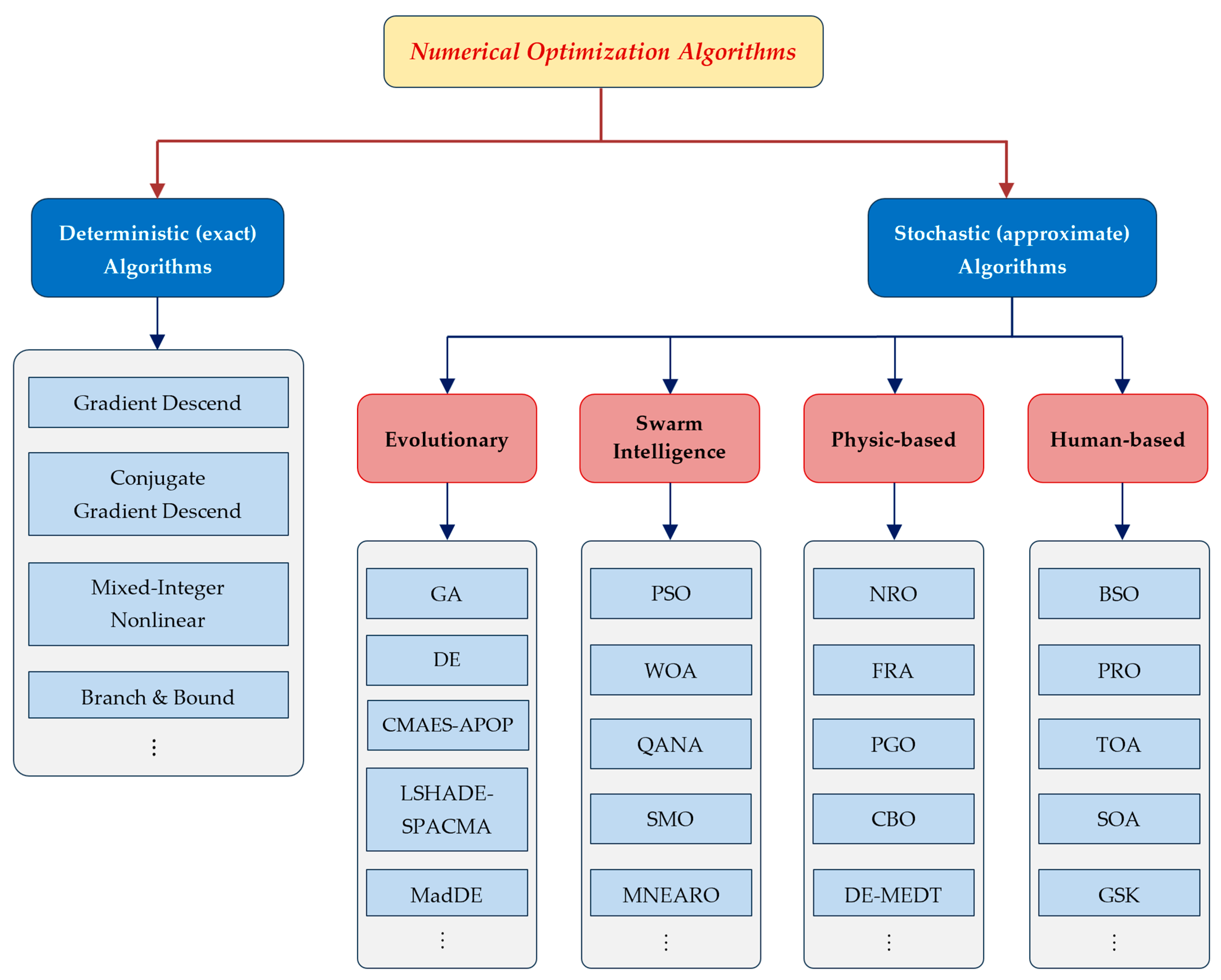
2. Literature Review
2.1. Metaheuristic Optimization Algorithms
2.2. GSK and Its Variants
2.2.1. Population Enhancement Techniques
2.2.2. Hybrid Algorithms
2.2.3. Strategy Enhancement Techniques
2.2.4. Composite Enhancement Techniques
2.3. Our Contributions Against the Existing Literature
3. Proposed ATMALS-GSK Algorithm
3.1. GSK
| Algorithm 1. Overall operation of original GSK Algorithm |
| Inputs: - N: Population size - D: Number of dimensions (decision variables) - K: Knowledge rate (controls the volume of knowledge exchange) - Kf: Knowledge factor (controls intensity of learning) - Kr: Knowledge ratio (probability of applying knowledge update) - MaxGen: Maximum number of generations - P: Proportion for grouping in senior phase Output: Global best solution (Xbest) 1 Initialize generation counter G ← 0 2 Generate an initial population of N individuals: 3 for 1 each i = 1:N 4 Initialize individual xi randomly in D-dimensional space 5 Evaluate fitness f (xi) for each individual i 6 for 2 each generation G = 1 to MaxGen: 7 Compute knowledge-sharing dimensions for both phases 8 Determine D(Junior) and D(Senior) using Equations (1) and (2). 9 Apply Junior Gaining–Sharing Knowledge Phase: 10 - For each individual i: 11 - Select nearest better (X_better) and worse (X_worse) individuals 12 - Choose a random peer (xr) for exploration 13 - Update D(Junior) dimensions based on the rules in Algorithm 2 14 Apply Senior Gaining–Sharing Knowledge Phase: 15 - Sort the population by fitness into Top P%, Middle N − 2P%, and Bottom P% 16 - For each individual i: 17 Select one peer from each group: X_best, X_mid, and X_worst 18 Update D(Senior) dimensions based on the rules in Algorithm 3 19 Evaluate new fitness values for all individuals 20 Update individuals based on new fitness: 21 Update the global best solution if a better one is found: 22 end for 2 23 end for 1 24 Return the global best solution found over all generations (X_best) |
3.1.1. Junior Phase
| Algorithm 2. Junior phase of GSK | |
| 1 | for 1 each solution i = 1:PopSize |
| 2 | for 2 each dimension j = 1:D |
| 3 | Generate a random number RND ∈ [0, 1] |
| 4 | if 1 RND ≤ Kr (Knowledge Ratio) |
| 5 | if 2 |
| 6 | ]; |
| 7 | else if 2 |
| 8 | ]; |
| 9 | end if 2 |
| 10 | else if 1 |
| 11 | ; |
| 12 | end if 1 |
| 13 | end for 2 |
| 14 | end for 1 |
3.1.2. Senior Phase
| Algorithm 3. Senior phase of GSK | |
| 1 | for 1 each individual i = 1:PopSize |
| 2 | for 2 each dimension j = 1:D |
| 3 | Generate a random number RND ∈ [0, 1] |
| 4 | if 1 (Knowledge Ratio) |
| 5 | if 2 |
| 6 | ]; |
| 7 | else if 2 |
| 8 | ]; |
| 9 | end if 2 |
| 10 | else if 1 |
| 11 | ; |
| 12 | end if 1 |
| 13 | end for 2 |
| 14 | end for 1 |
3.2. ATMALS-GSK
- Lack of generalizability across problem domains: Fixed parameter values might yield strong results for a particular problem but often fail to perform well across different problem settings or objective landscapes. What works for a scheduling problem, for instance, may underperform in a continuous optimization task.
- Inflexibility across search stages: The same parameter values are used throughout the entire execution of the algorithm, from the initial exploration phase to the final convergence phase. However, different phases of the search process typically benefit from different behaviors—strong exploration in early generations and refined exploitation in later ones. Static parameters fail to accommodate this shift, potentially leading to premature convergence or excessive wandering.
- No feedback from historical performance: The original GSK lacks a learning mechanism to leverage past search experience. Without any form of memory or adaptive control, the algorithm is unable to assess the effectiveness of different parameter configurations over time. This absence of self-tuning prevents the algorithm from evolving and improving its own strategy dynamically.
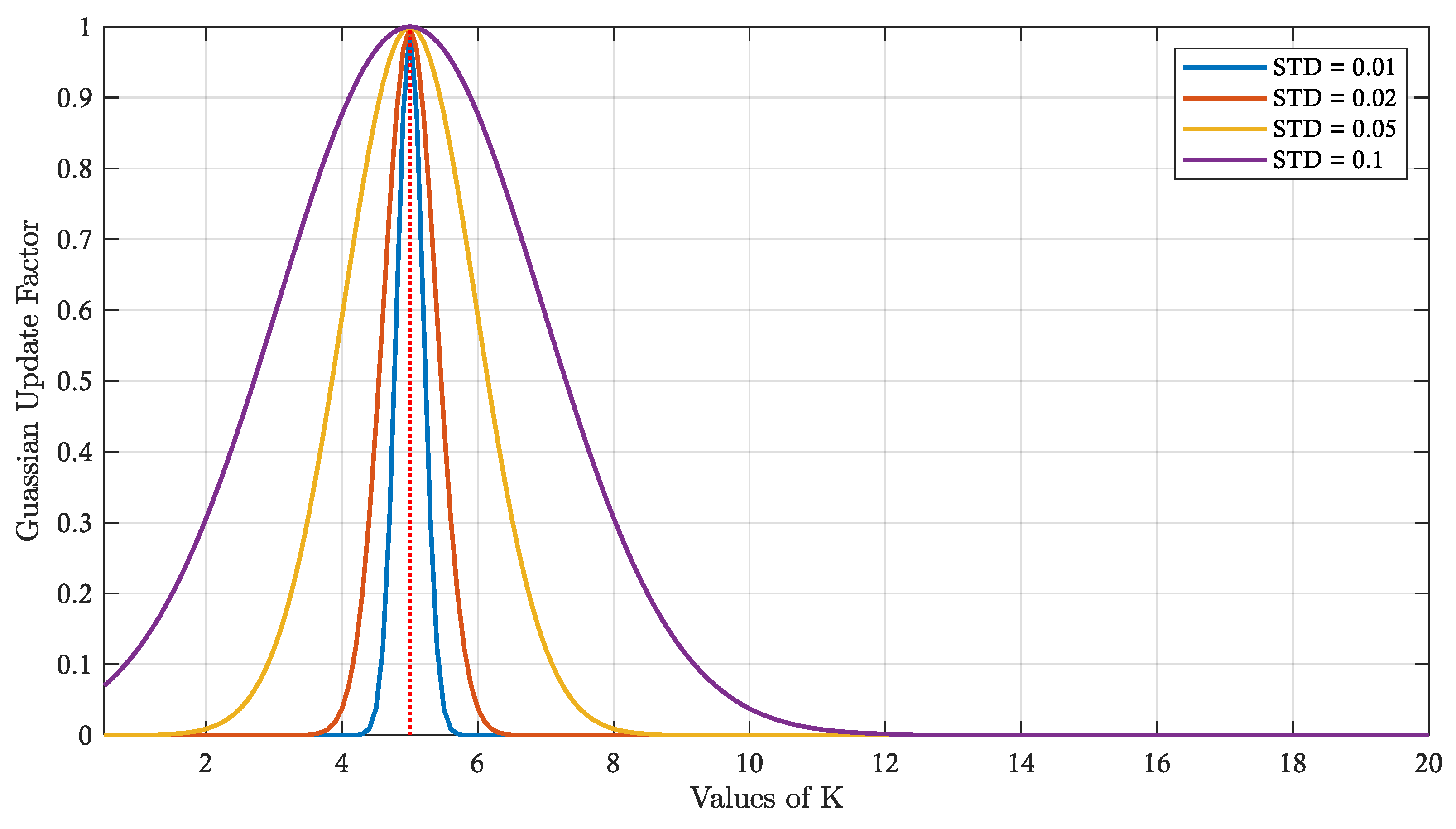
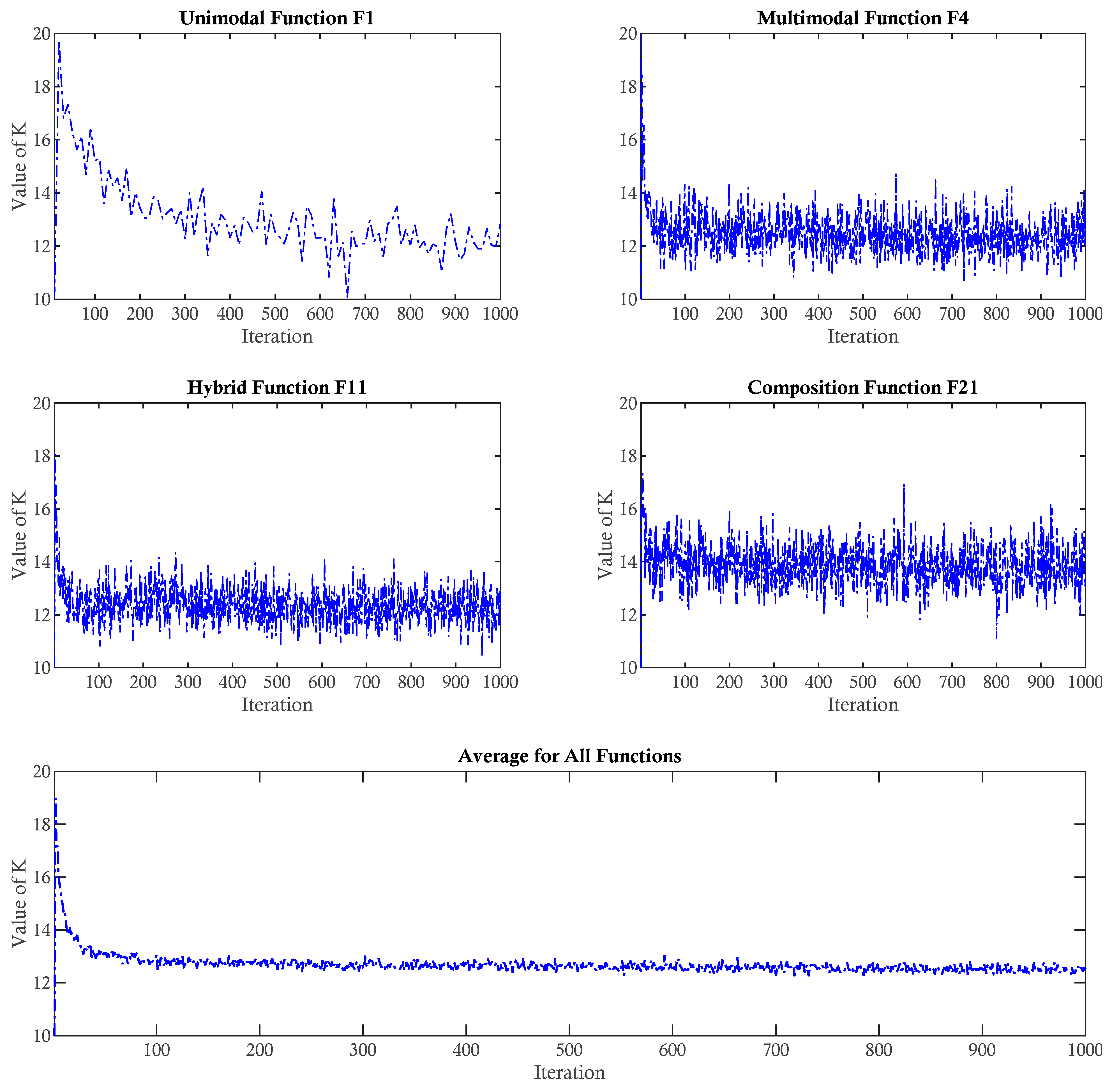
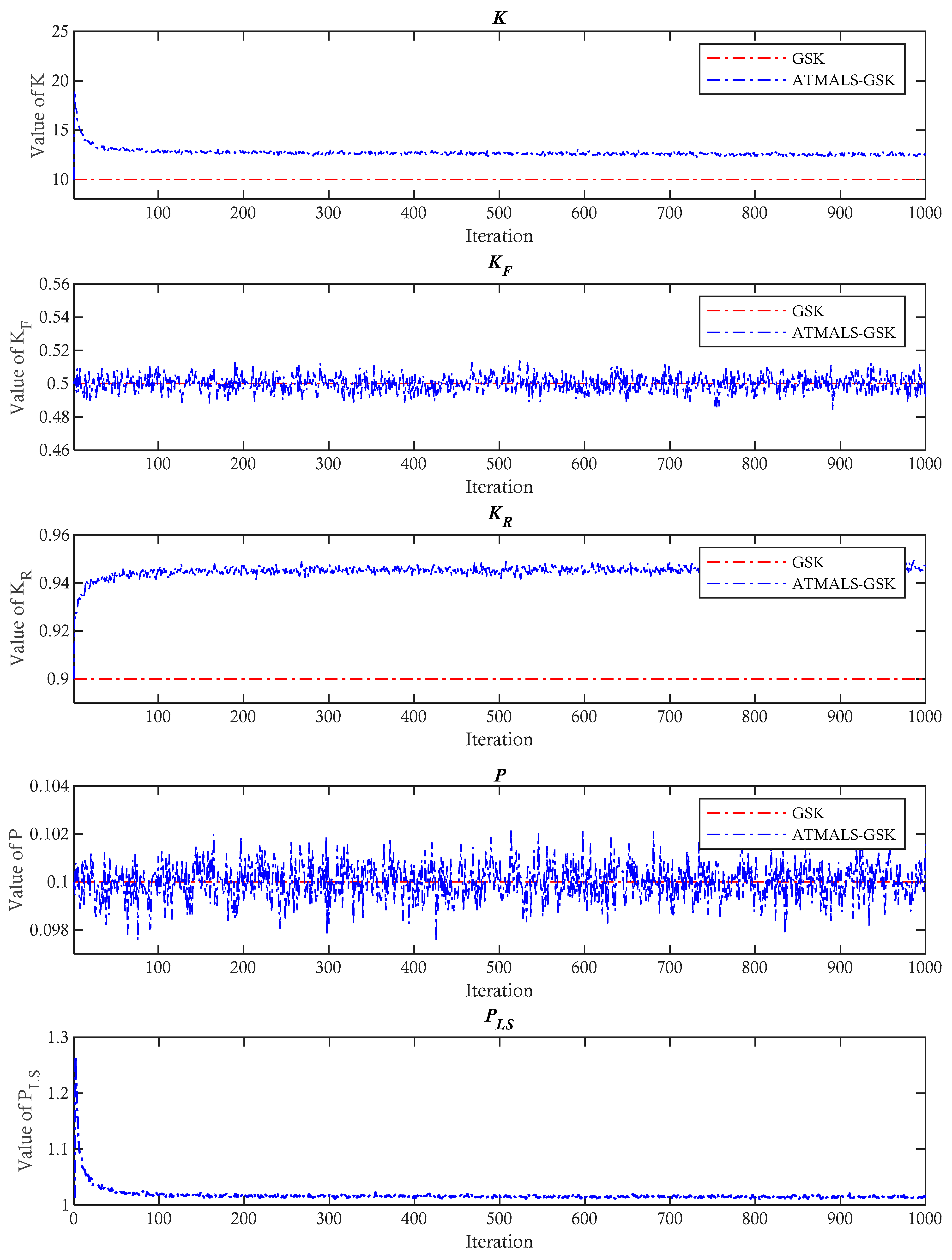
3.2.1. Adaptive K
3.2.2. Adaptive Kr
3.2.3. Adaptive Kf
3.2.4. Adaptive P
3.2.5. Adaptive PLS
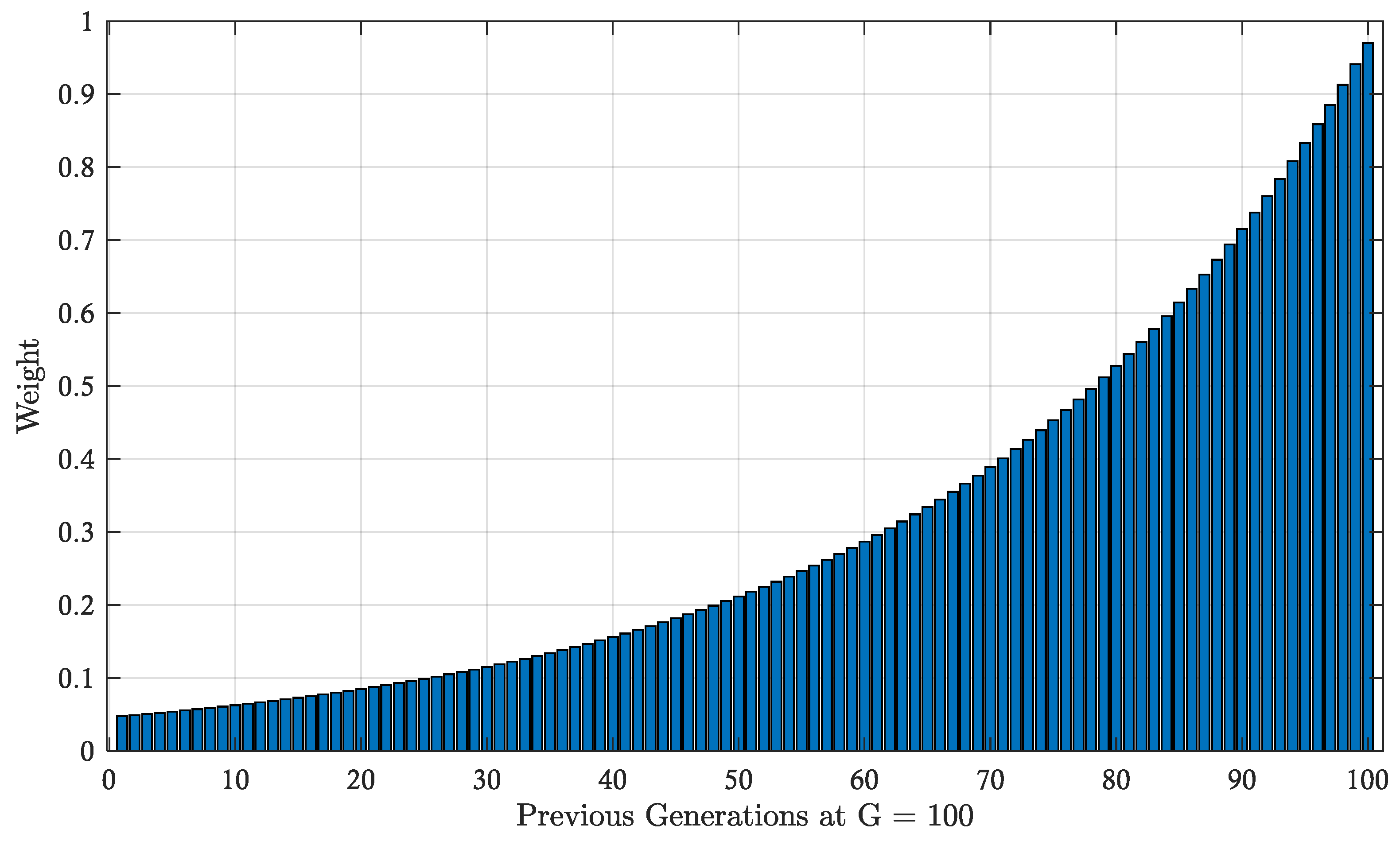
3.2.6. Overall Operation of ATMALS-GSK
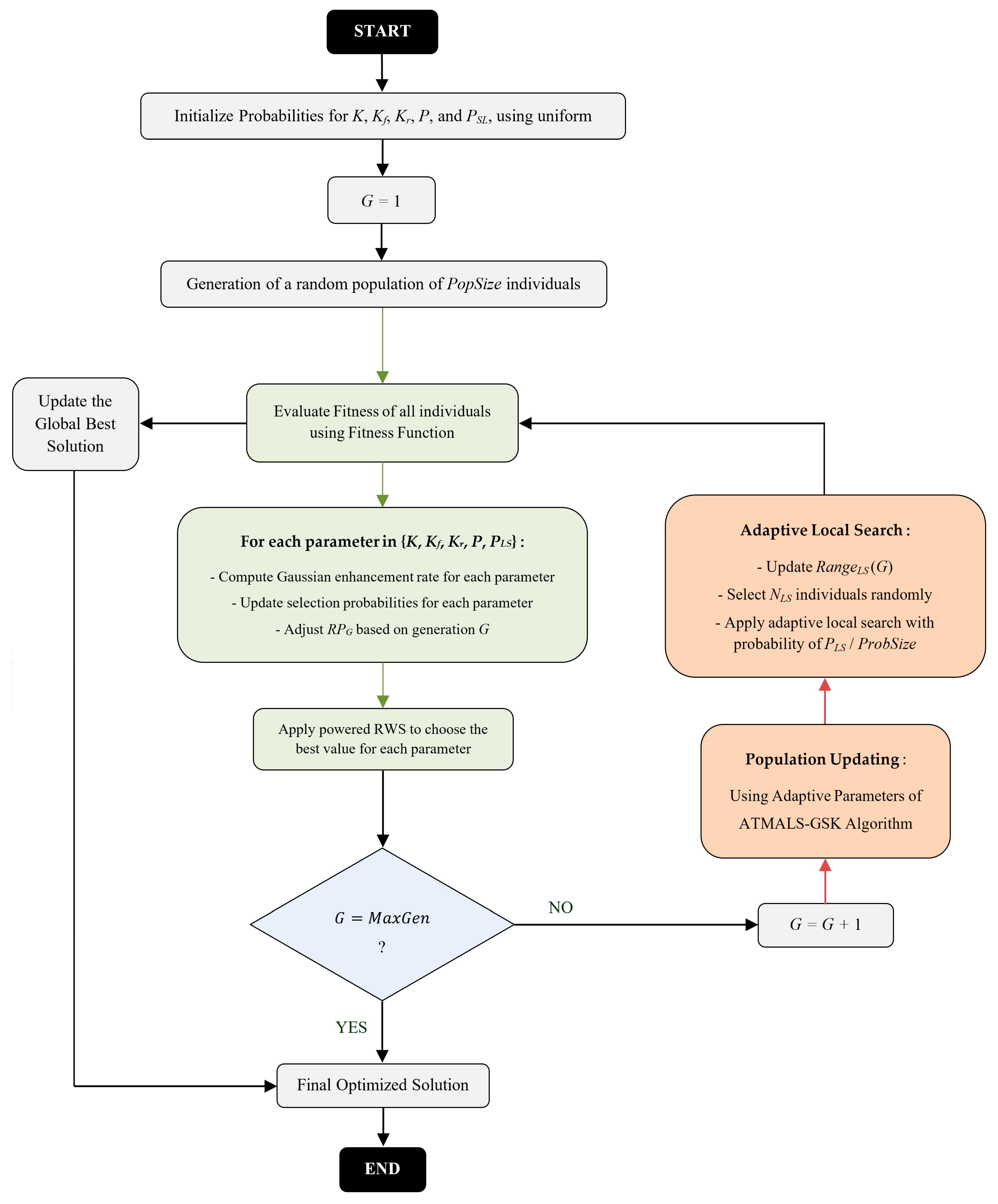
| Algorithm 4. Proposed ATMALS-GSK Algorithm |
| Inputs: - MaxGen: Maximum generations - PopSize: Population size - ProbSize: Problem dimension - Fitness(): Objective function to minimize - KVALUES ← [1, 2, 3, …, 30] - KfVALUES ← [0.2, 0.3, …, 0.8] - KrVALUES ← [0.8, 0.81, …, 1.0] - PVALUES ← [0.05, 0.06, …, 0.2] - PLSVALUES ← [0.1, 0.11, …, 0.2] Initialize Probabilities for K, Kf, Kr, P, and PSL, using uniform distribution Initialize RPG ← 1, NLS ← 0.05 × PopSize, α ← 0.97, δ ← 0.05 × (max(VALUES) − min(VALUES)) Main ATMALS-GSK Algorithm: 1 Initialize population of PopSize individuals randomly 2 for 1 generation G = 1 to MaxGen do: 3 Evaluate Fitness of all individuals 4 for 2 each parameter in {K, Kf, Kr, P, PLS} do: 5 Compute Gaussian enhancement rate based on Equations (3) and (4) 6 Update selection probabilities using Equation (5) 7 Apply powered RWS using Equations (6) and (7) to choose parameter values 8 end for 2 9 RPG ← Adjust RPG based on generation G (gradual increase) 10 Partition individuals into Junior and Senior based on adaptive Kr value 11 for 3 each individual i in population do: 12 if i is in Junior group then: 13 Update D(junior) using junior learning rule (based on K) 14 else if i is in Senior group then: 15 Update D(senior) using senior learning rule (based on K) 16 end if 17 end for 3 18 Update RangeLS(G) using Equation (8) 19 Select NLS individuals randomly 20 for 4 each selected individual in NLS do: 21 for 5 each dimension d do: 22 Apply adaptive local search with probability of PLS/ProbSize 23 end for 5 24 end for 4 25 Update historical memory of parameters’ fitness improvements 26 Update the global best solution found so far 27 end for 1 Output: Best solution found and its fitness value |
4. Performance Evaluation
4.1. Settings
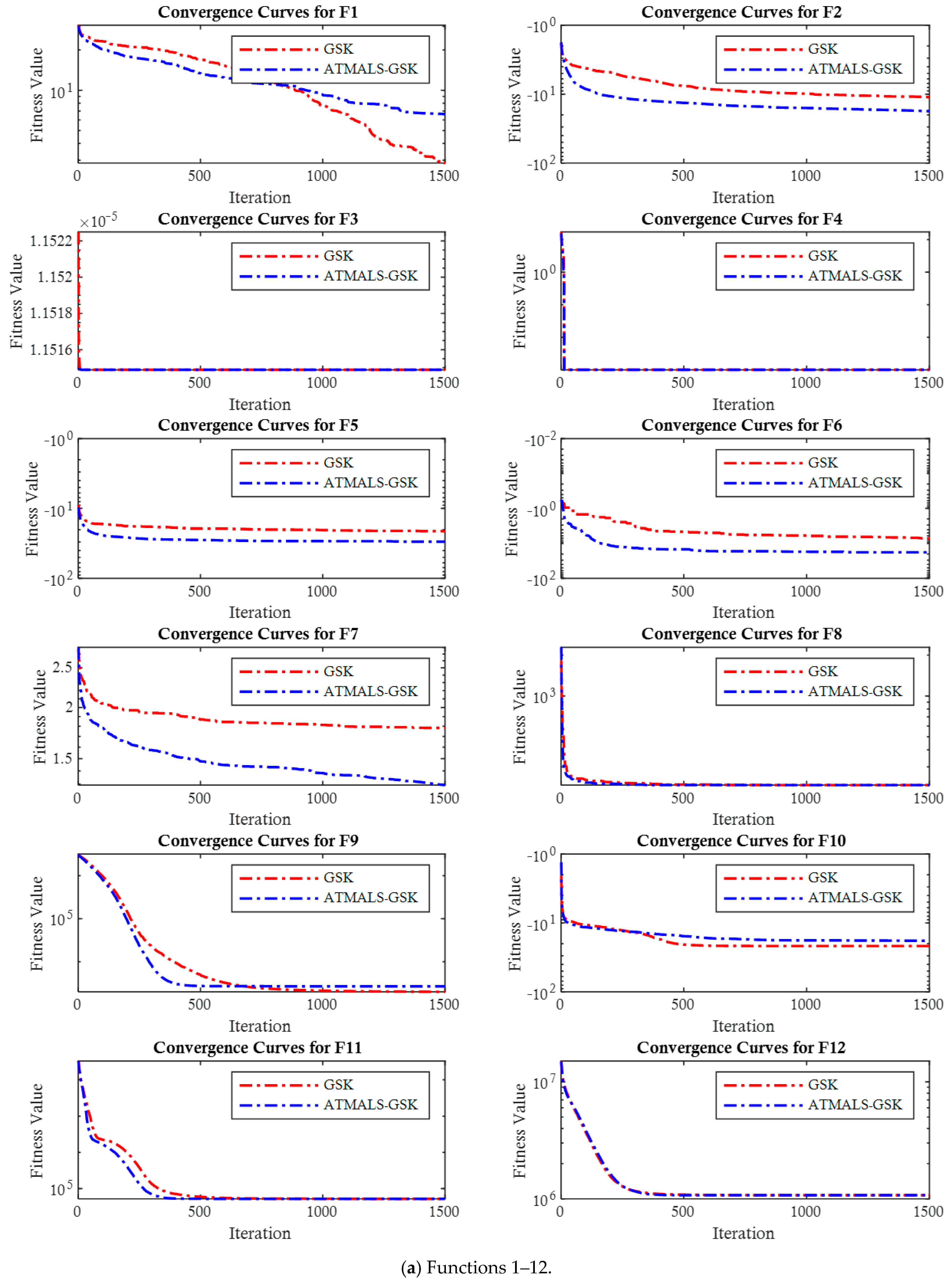
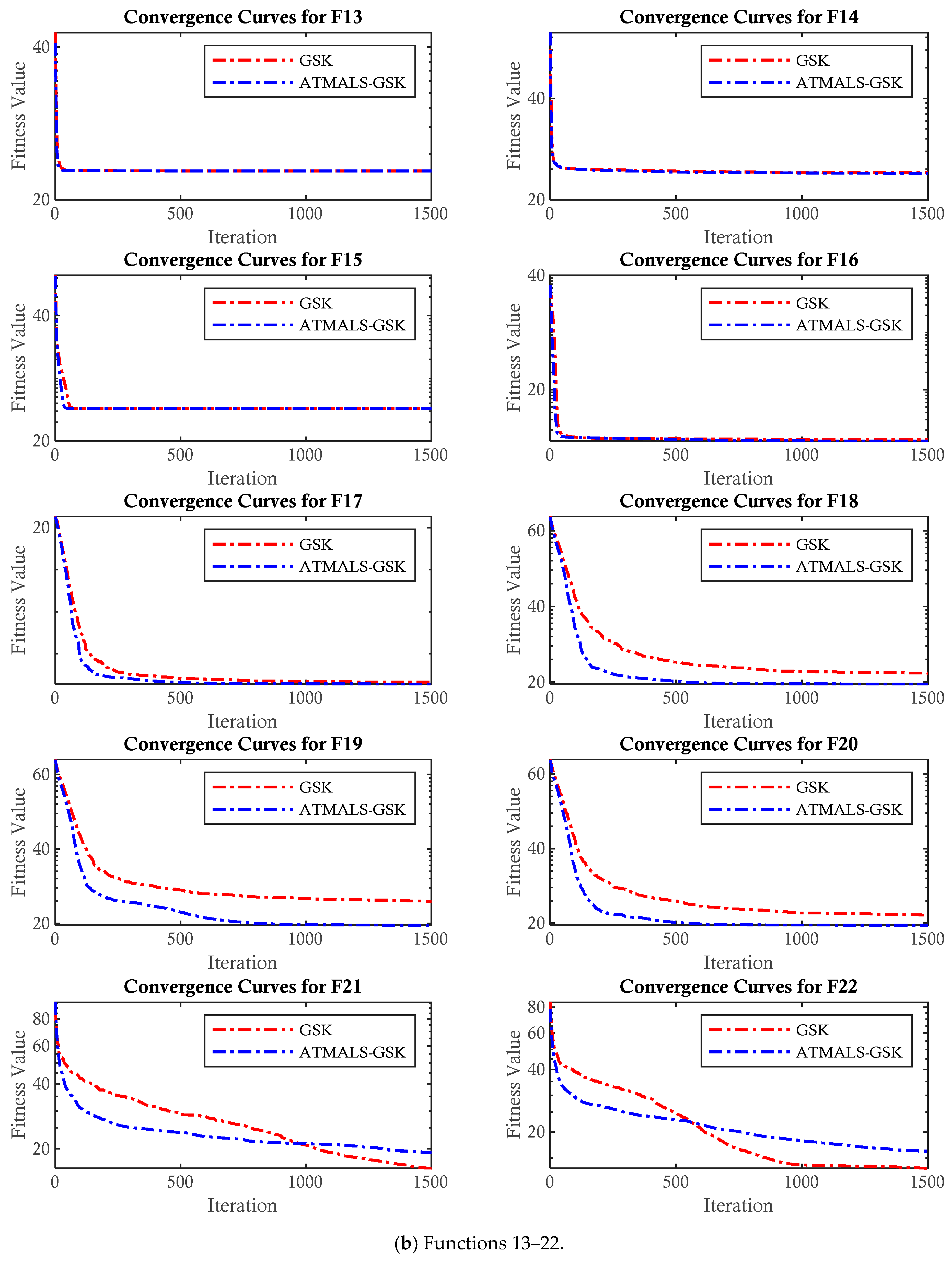
4.2. Results of ATMALS-GSK
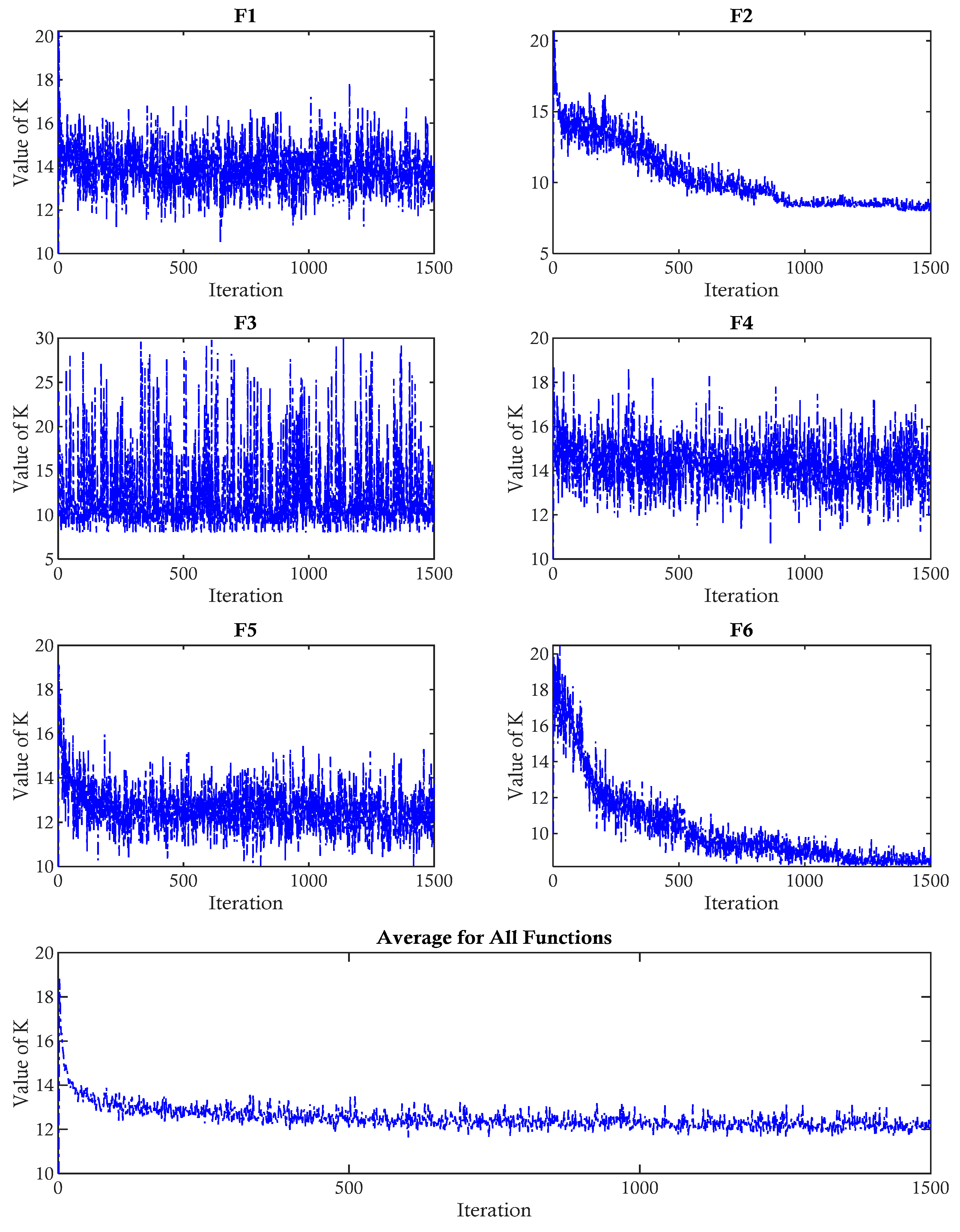
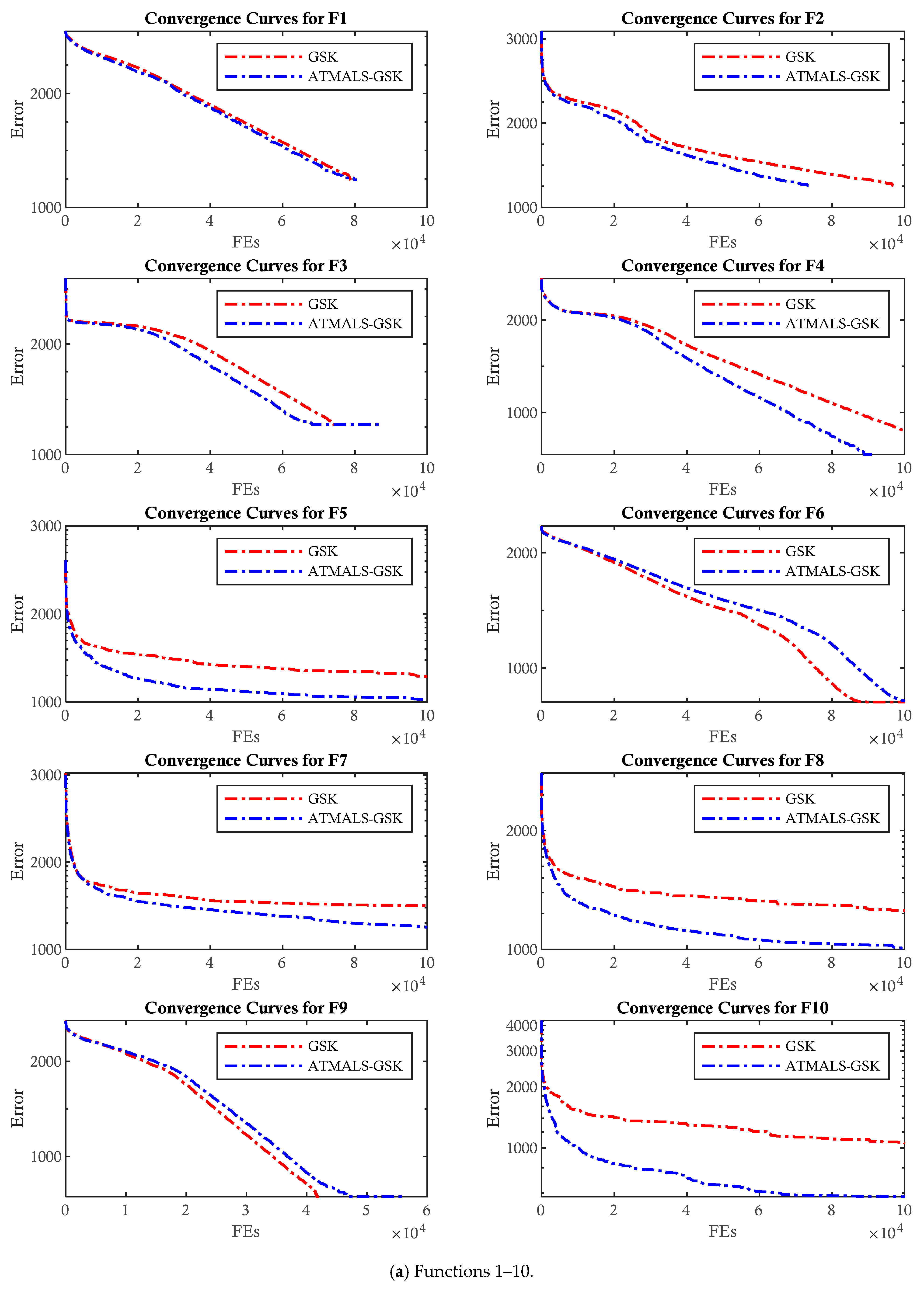
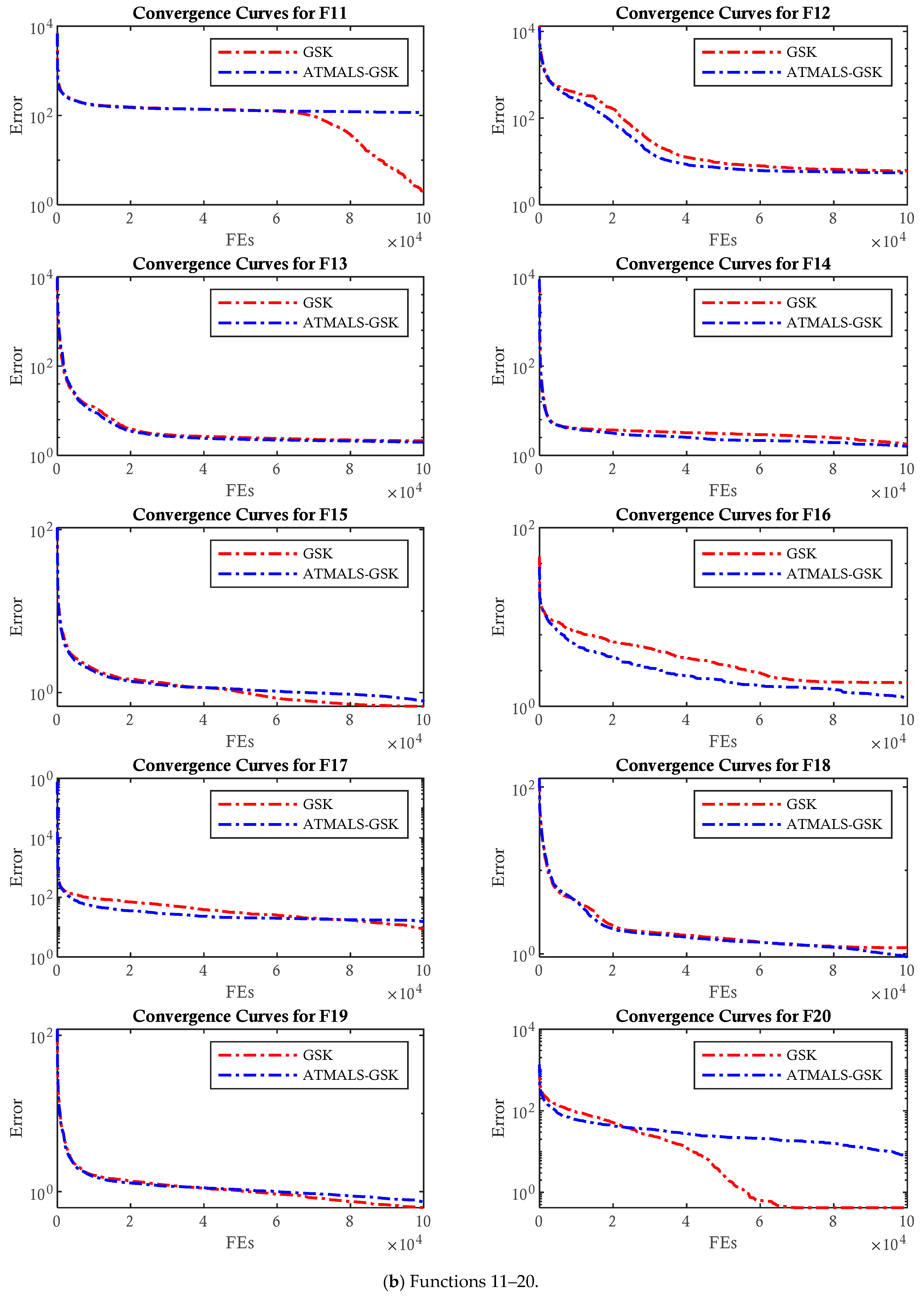
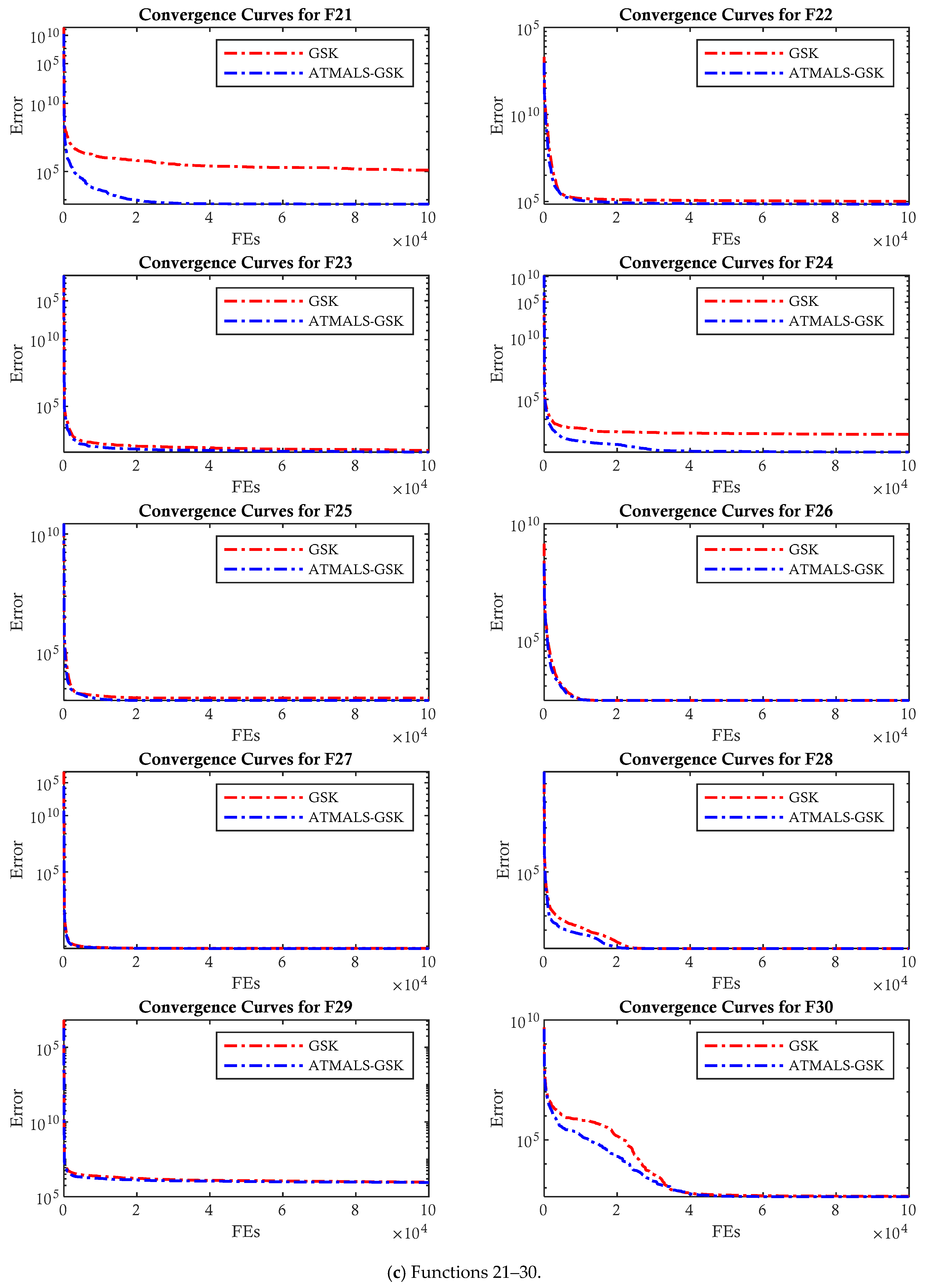
4.2.1. CEC 2011
4.2.2. CEC 2017
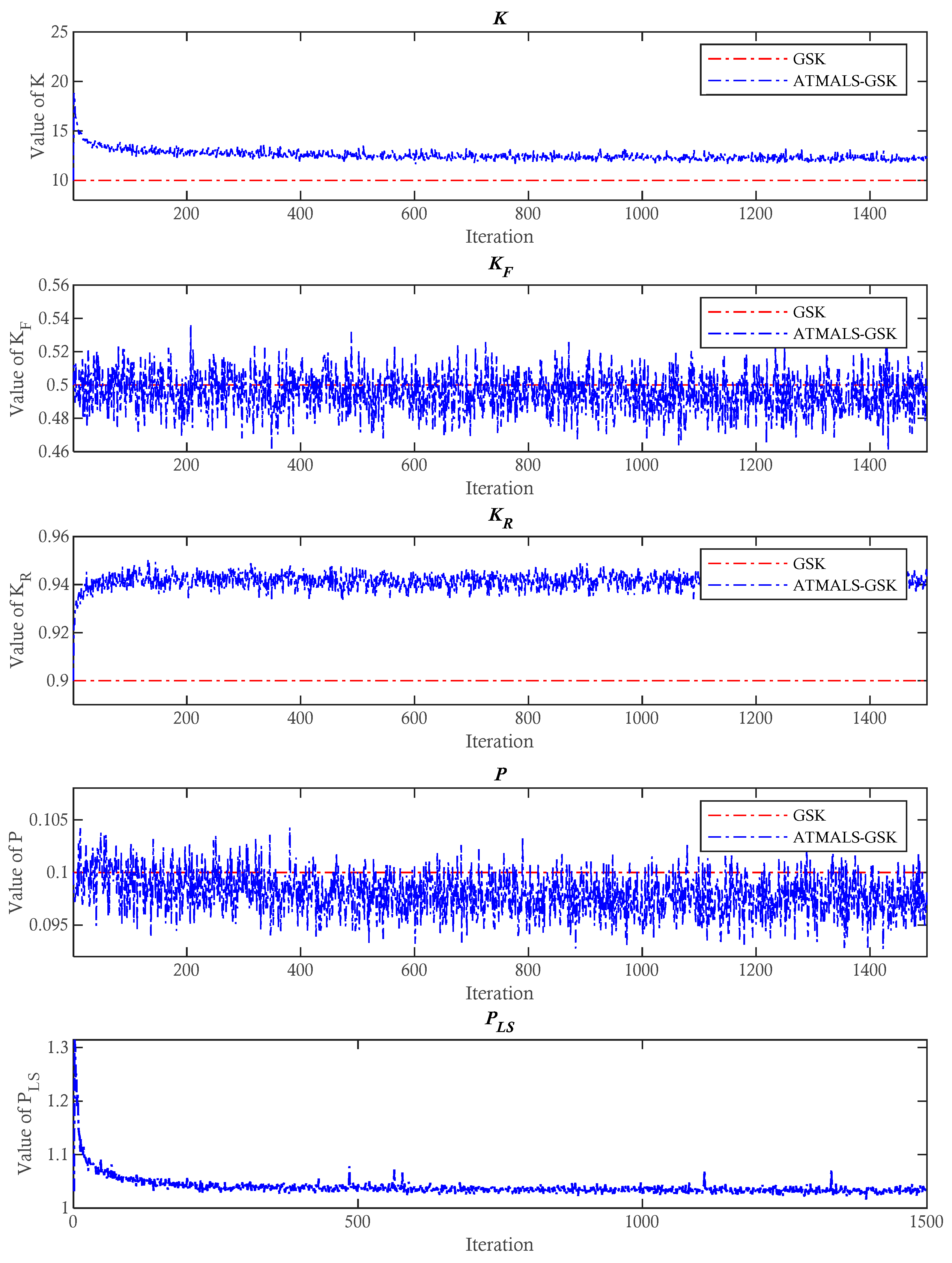
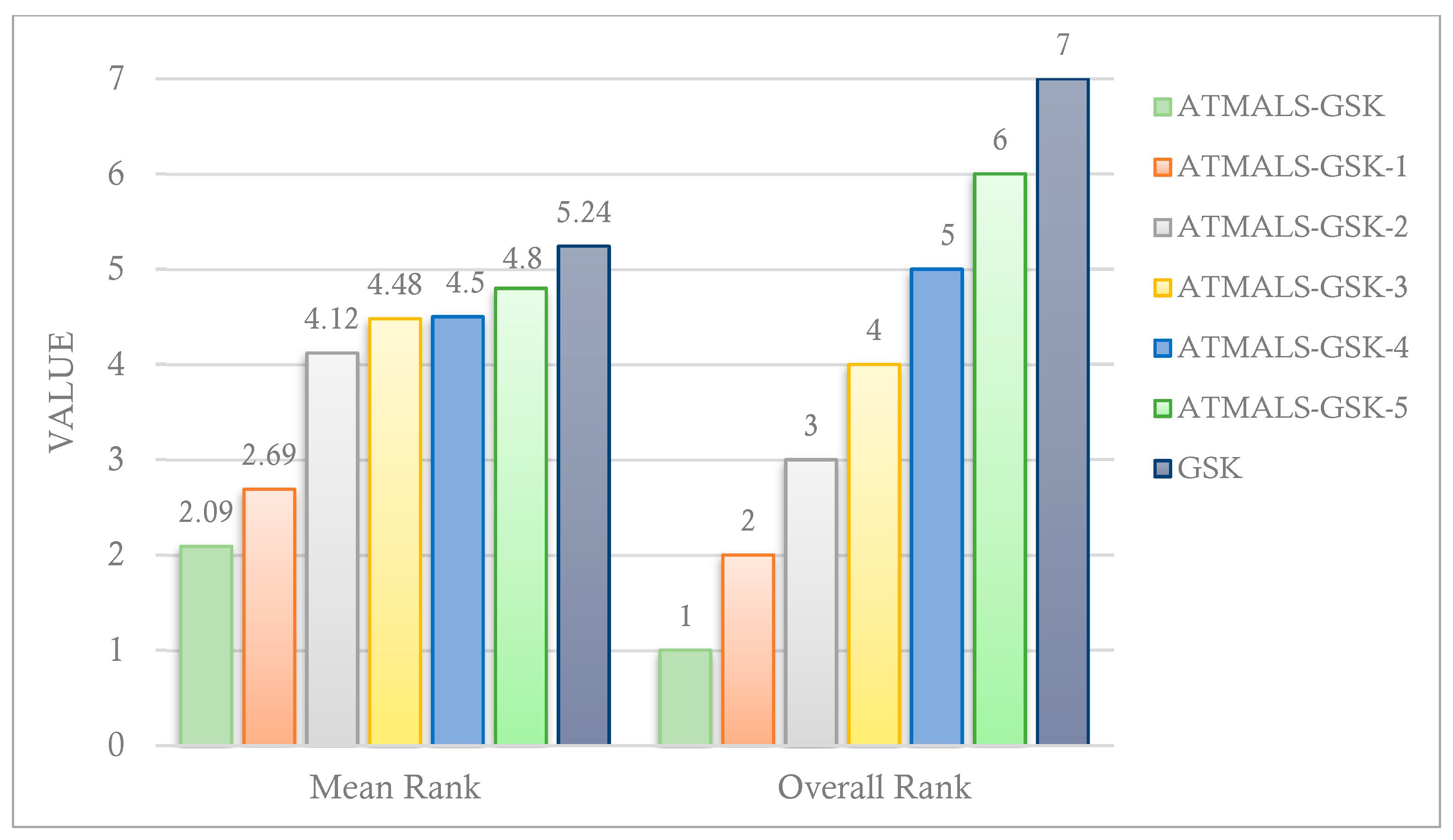
4.3. Comparison with GSK and Modified GSKs
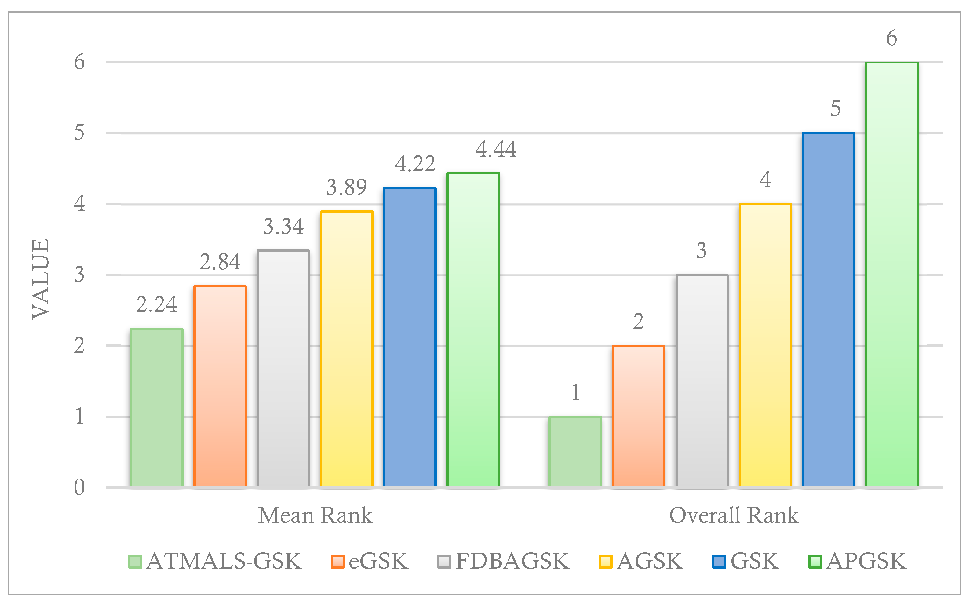
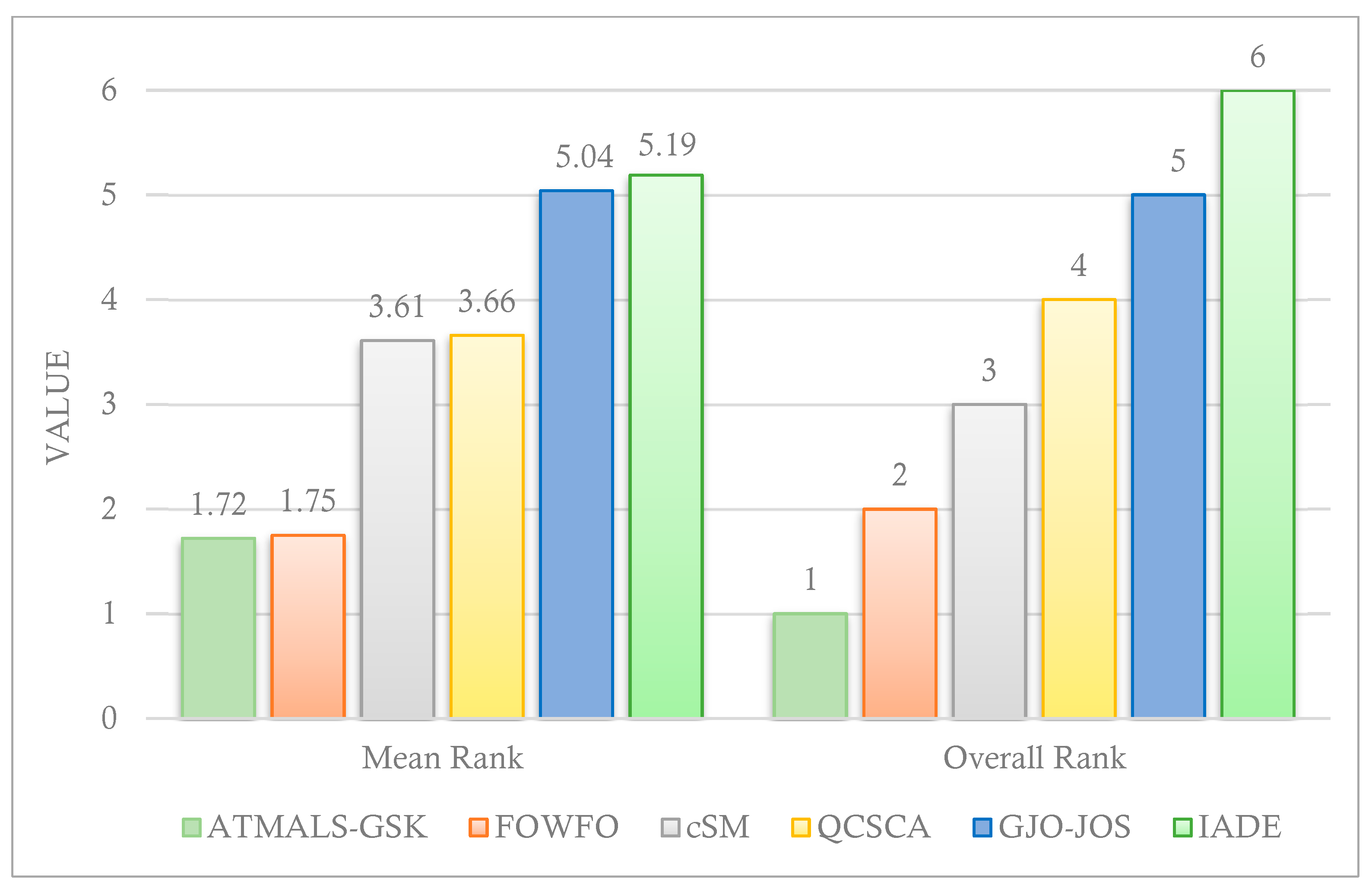
4.4. Comparison with Other Metaheuristic Algorithms
4.5. Statistical Analysis
4.6. Parametric Study of ATMALS-GSK
5. Conclusions
Author Contributions
Funding
Data Availability Statement
Conflicts of Interest
References
- Selvarajan, S. A comprehensive study on modern optimization techniques for engineering applications. Artif. Intell. Rev. 2024, 57, 194. [Google Scholar] [CrossRef]
- Deng, J.; Zhou, C.; Wang, J. Approaches and application of heat and water network integration in chemical process system engineering: A review. Chem. Eng. Process.-Process Intensif. 2023, 183, 109263. [Google Scholar] [CrossRef]
- Fanian, F.; Rafsanjani, M.K.; Shokouhifar, M. Combined fuzzy-metaheuristic framework for bridge health monitoring using UAV-enabled rechargeable wireless sensor networks. Appl. Soft Comput. 2024, 167, 112429. [Google Scholar] [CrossRef]
- Shokouhifar, M.; Fanian, F.; Rafsanjani, M.K.; Hosseinzadeh, M.; Mirjalili, S. AI-driven cluster-based routing protocols in WSNs: A survey of fuzzy heuristics, metaheuristics, and machine learning models. Comput. Sci. Rev. 2024, 54, 100684. [Google Scholar] [CrossRef]
- Memarian, S.; Behmanesh-Fard, N.; Aryai, P.; Shokouhifar, M.; Mirjalili, S.; del Carmen Romero-Ternero, M. TSFIS-GWO: Metaheuristic-driven takagi-sugeno fuzzy system for adaptive real-time routing in WBANs. Appl. Soft Comput. 2024, 155, 111427. [Google Scholar] [CrossRef]
- Xie, L.; Wang, Y.; Tang, S.; Li, Y.; Zhang, Z.; Huang, C. Adaptive gaining-sharing knowledge-based variant algorithm with historical probability expansion and its application in escape maneuver decision making. Artif. Intell. Rev. 2025, 58, 1–43. [Google Scholar] [CrossRef]
- Janga Reddy, M.; Nagesh Kumar, D. Evolutionary algorithms, swarm intelligence methods, and their applications in water resources engineering: A state-of-the-art review. H2Open J. 2020, 3, 135–188. [Google Scholar] [CrossRef]
- Shokouhifar, M. FH-ACO: Fuzzy heuristic-based ant colony optimization for joint virtual network function placement and routing. Appl. Soft Comput. 2021, 107, 107401. [Google Scholar] [CrossRef]
- Siddique, N.; Adeli, H. Physics-based search and optimization: Inspirations from nature. Expert Syst. 2016, 33, 607–623. [Google Scholar] [CrossRef]
- Emami, H. Stock exchange trading optimization algorithm: A human-inspired method for global optimization. J. Supercomput. 2022, 78, 2125–2174. [Google Scholar] [CrossRef]
- Tanweer, M.R.; Sundaram, S. Human cognition inspired particle swarm optimization algorithm. In Proceedings of the 2014 IEEE Ninth International Conference on Intelligent Sensors, Sensor Networks and Information Processing, Singapore, 21–24 April 2014; pp. 1–6. [Google Scholar]
- Debnath, S.; Arif, W.; Baishya, S. Buyer inspired meta-heuristic optimization algorithm. Open Comput. Sci. 2020, 10, 194–219. [Google Scholar] [CrossRef]
- Liu, C.; Ma, Y.; Yin, H.; Yu, L. Human resource allocation for multiple scientific research projects via improved pigeon-inspired optimization algorithm. Sci. China Technol. Sci. 2021, 64, 139–147. [Google Scholar] [CrossRef]
- Veysari, E.F. A new optimization algorithm inspired by the quest for the evolution of human society: Human felicity algorithm. Expert Syst. Appl. 2022, 193, 116468. [Google Scholar]
- Liu, Z.; Jian, X.; Sadiq, T.; Shaikh, Z.A.; Alfarraj, O.; Alblehai, F.; Tolba, A. Efficient control of spider-like medical robots with capsule neural networks and modified spring search algorithm. Sci. Rep. 2025, 15, 13828. [Google Scholar] [CrossRef] [PubMed]
- Mohamed, A.W.; Hadi, A.A.; Mohamed, A.K. Gaining-sharing knowledge based algorithm for solving optimization problems: A novel nature-inspired algorithm. Int. J. Mach. Learn. Cybern. 2020, 11, 1501–1529. [Google Scholar] [CrossRef]
- Nguyen, D.M. The effect of mirrored sampling with active CMA and sample reuse in the CMAES-APOP algorithm. In Proceedings of the Genetic and Evolutionary Computation Conference Companion, Boston, MA, USA, 9–13 July 2022; pp. 403–406. [Google Scholar]
- Gao, Y.; Zhang, J.; Wang, Y.; Wang, J.; Qin, L. Love evolution algorithm: A stimulus–value–role theory-inspired evolutionary algorithm for global optimization. J. Supercomput. 2024, 80, 12346–12407. [Google Scholar] [CrossRef]
- Biswas, S.; Saha, D.; De, S.; Cobb, A.D.; Das, S.; Jalaian, B.A. Improving differential evolution through Bayesian hyperparameter optimization. In Proceedings of the 2021 IEEE Congress on Evolutionary Computation, Kraków, Poland, 28 June–1 July 2021; pp. 832–840. [Google Scholar]
- Kennedy, J.; Eberhart, R. Particle swarm optimization. In Proceedings of the ICNN’95-International Conference on Neural Networks, Perth, WA, Australia, 27 November–1 December 1995; Volume 4, pp. 1942–1948. [Google Scholar]
- Mirjalili, S.; Lewis, A. The whale optimization algorithm. Adv. Eng. Softw. 2016, 95, 51–67. [Google Scholar] [CrossRef]
- Zamani, H.; Nadimi-Shahraki, M.H.; Gandomi, A.H. QANA: Quantum-based avian navigation optimizer algorithm. Eng. Appl. Artif. Intell. 2021, 104, 104314. [Google Scholar] [CrossRef]
- Zamani, H.; Nadimi-Shahraki, M.H.; Gandomi, A.H. Starling murmuration optimizer: A novel bio-inspired algorithm for global and engineering optimization. Comput. Methods Appl. Mech. Eng. 2022, 392, 114616. [Google Scholar] [CrossRef]
- Jangir, P.; Ezugwu, A.E.; Saleem, K.; Arpita Agrawal, S.P.; Pandya, S.B.; Parmar, A.; Gulothungan, G.; Abualigah, L. A hybrid mutational Northern Goshawk and elite opposition learning artificial rabbits optimizer for PEMFC parameter estimation. Sci. Rep. 2024, 14, 28657. [Google Scholar] [CrossRef]
- Wei, Z.; Huang, C.; Wang, X.; Han, T.; Li, Y. Nuclear reaction optimization: A novel and powerful physics-based algorithm for global optimization. IEEE Access 2019, 7, 66084–66109. [Google Scholar] [CrossRef]
- Tahani, M.; Babayan, N. Flow Regime Algorithm (FRA): A physics-based meta-heuristics algorithm. Knowl. Inf. Syst. 2019, 60, 1001–1038. [Google Scholar] [CrossRef]
- Kaveh, A.; Akbari, H.; Hosseini, S.M. Plasma generation optimization: A new physically-based metaheuristic algorithm for solving constrained optimization problems. Eng. Comput. 2021, 38, 1554–1606. [Google Scholar] [CrossRef]
- Chen, D.; Lu, R.; Li, S.; Zou, F.; Liu, Y. An enhanced colliding bodies optimization and its application. Artif. Intell. Rev. 2020, 53, 1127–1186. [Google Scholar] [CrossRef]
- Kaveh, A.; Hosseini, S.M.; Zaerreza, A. A physics-based metaheuristic algorithm based on doppler effect phenomenon and mean euclidian distance threshold. Period. Polytech. Civ. Eng. 2022, 66, 820–842. [Google Scholar] [CrossRef]
- Shi, Y. Brain storm optimization algorithm. In Advances in Swarm Intelligence: Second International Conference, ICSI 2011, Chongqing, China, June 12–15, 2011, Proceedings, Part I; Springer: Berlin/Heidelberg, Germany, 2011; pp. 303–309. [Google Scholar]
- Moosavi, S.H.S.; Bardsiri, V.K. Poor and rich optimization algorithm: A new human-based and multi populations algorithm. Eng. Appl. Artif. Intell. 2019, 86, 165–181. [Google Scholar] [CrossRef]
- Dehghani, M.; Trojovský, P. Teamwork optimization algorithm: A new optimization approach for function minimization/maximization. Sensors 2021, 21, 4567. [Google Scholar] [CrossRef]
- Givi, H.; Hubalovska, M. Skill Optimization Algorithm: A New Human-Based Metaheuristic Technique. Comput. Mater. Contin. 2023, 74, 179–202. [Google Scholar] [CrossRef]
- Jalali, S.M.J.; Ahmadian, M.; Ahmadian, S.; Khosravi, A.; Alazab, M.; Nahavandi, S. An oppositional-Cauchy based GSK evolutionary algorithm with a novel deep ensemble reinforcement learning strategy for COVID-19 diagnosis. Appl. Soft Comput. 2021, 111, 107675. [Google Scholar] [CrossRef]
- Ma, H.; Zhang, J.; Wei, W.; Cheng, W.; Liu, Q. A Modified Gaining-Sharing Knowledge Algorithm Based on Dual-Population and Multi-operators for Unconstrained Optimization. In Advances in Swarm Intelligence: Second International Conference, ICSI 2011, Chongqing, China, June 12–15, 2011, Proceedings, Part I; Springer Nature: Cham, Switzerland, 2023; pp. 309–319. [Google Scholar]
- Bakır, H.; Duman, S.; Guvenc, U.; Kahraman, H.T. Improved adaptive gaining-sharing knowledge algorithm with FDB-based guiding mechanism for optimization of optimal reactive power flow problem. Electr. Eng. 2023, 105, 3121–3160. [Google Scholar] [CrossRef]
- Pan, J.S.; Liu, L.F.; Chu, S.C.; Song, P.C.; Liu, G.G. A new gaining-sharing knowledge based algorithm with parallel opposition-based learning for Internet of Vehicles. Mathematics 2023, 11, 2953. [Google Scholar] [CrossRef]
- Kamarposhti, M.A.; Shokouhandeh, H.; Lee, Y.; Kang, S.K.; Colak, I.; Barhoumi, E.M. Optimizing switch placement and status for sustainable grid operation and effective distributed generation integration using the APGSK-IMODE algorithm. Int. J. Low-Carbon Technol. 2024, 19, 2676–2686. [Google Scholar] [CrossRef]
- Liang, Z.; Wang, Z. Enhancing population diversity based gaining-sharing knowledge based algorithm for global optimization and engineering design problems. Expert Syst. Appl. 2024, 252, 123958. [Google Scholar] [CrossRef]
- Nabahat, M.; Khiyabani, F.M.; Navmipour, N.J. Hybrid Noise Reduction Filter Using the Gaining–Sharing Knowledge-Based Optimization and the Whale Optimization Algorithms. SN Comput. Sci. 2024, 5, 417. [Google Scholar] [CrossRef]
- Nunes, H.; Pombo, J.; Mariano, S.; do Rosário Calado, M. Parameter Estimation of Lithium-Ion Batteries Using GSKPSO Hybrid Method Based on Impedance Data. In Proceedings of the 2024 IEEE International Conference on Environment and Electrical Engineering and 2024 IEEE Industrial and Commercial Power Systems Europe (EEEIC/I&CPS Europe), Rome, Italy, 17–20 June 2024; pp. 1–6. [Google Scholar]
- Zhong, X.; Duan, M.; Zhang, X.; Cheng, P. A hybrid differential evolution based on gaining-sharing knowledge algorithm and harris hawks optimization. PLoS ONE 2021, 16, e0250951. [Google Scholar] [CrossRef] [PubMed]
- Navaneetha Krishnan, M.; Thiyagarajan, R. Multi-objective task scheduling in fog computing using improved gaining sharing knowledge based algorithm. Concurr. Comput. Pract. Exp. 2022, 34, e7227. [Google Scholar] [CrossRef]
- Liang, Z.; Shu, T.; Ding, Z. A novel improved whale optimization algorithm for global optimization and engineering applications. Mathematics 2024, 12, 636. [Google Scholar] [CrossRef]
- Mohamed, A.W.; Abutarboush, H.F.; Hadi, A.A.; Mohamed, A.K. Gaining-sharing knowledge based algorithm with adaptive parameters for engineering optimization. IEEE Access 2021, 9, 65934–65946. [Google Scholar] [CrossRef]
- Mohamed, A.W.; Hadi, A.A.; Mohamed, A.K.; Awad, N.H. Evaluating the performance of adaptive gainingsharing knowledge based algorithm on CEC 2020 benchmark problems. In Proceedings of the 2020 IEEE Congress on Evolutionary Computation, Glasgow, UK, 19–24 July 2020; pp. 1–8. [Google Scholar]
- Hodashinsky, I.A. Methods for improving the efficiency of swarm optimization algorithms. A survey. Autom. Remote Control 2020, 82, 935–967. [Google Scholar] [CrossRef]
- Sadeghi, A.; Daneshvar, A.; Zaj, M.M. Combined ensemble multi-class SVM and fuzzy NSGA-II for trend forecasting and trading in Forex markets. Expert Syst. Appl. 2021, 185, 115566. [Google Scholar] [CrossRef]
- Jawad, M.A.; Roshdy, H.S.M.; Mohamed, A.W. Enhanced Gaining-Sharing Knowledge-based algorithm. Results Control Optim. 2025, 19, 100542. [Google Scholar] [CrossRef]
- Zhou, Z.; Shojafar, M.; Abawajy, J.; Bashir, A.K. IADE: An improved differential evolution algorithm to preserve sustainability in a 6G network. IEEE Trans. Green Commun. Netw. 2021, 5, 1747–1760. [Google Scholar] [CrossRef]
- Arini, F.Y.; Sunat, K.; Soomlek, C. Golden jackal optimization with joint opposite selection: An enhanced nature-inspired optimization algorithm for solving optimization problems. IEEE Access 2022, 10, 128800–128823. [Google Scholar] [CrossRef]
- Hu, H.; Shan, W.; Tang, Y.; Heidari, A.A.; Chen, H.; Liu, H.; Wang, M.; Escorcia-Gutierrez, J.; Mansour, R.F.; Chen, J. Horizontal and vertical crossover of sine cosine algorithm with quick moves for optimization and feature selection. J. Comput. Des. Eng. 2022, 9, 2524–2555. [Google Scholar] [CrossRef]
- Khalfi, S.; Iacca, G.; Draa, A. A single-solution–compact hybrid algorithm for continuous optimization. Memetic Comput. 2023, 15, 155–204. [Google Scholar] [CrossRef]
- Tang, Z.; Wang, K.; Zang, Y.; Zhu, Q.; Todo, Y.; Gao, S. Fractional-order water flow optimizer. Int. J. Comput. Intell. Syst. 2024, 17, 84. [Google Scholar] [CrossRef]
- Das, S.; Suganthan, P.N. Problem Definitions and Evaluation Criteria for CEC 2011 Competition on Testing Evolutionary Algorithms on Real World Optimization Problems; Technical Report; Jadavpur University: Kolkata, India; Nanyang Technological University: Singapore, 2010. [Google Scholar]
- Awad, N.H.; Ali, M.Z.; Liang, J.J.; Qu, B.Y.; Suganthan, P.N. Problem Definitions and Evaluation Criteria for the CEC 2017 Special Session and Competition on Single Objective Bound Constrained Real-Parameter Numerical Optimization; Technical Report; Nanyang Technological University: Singapore, 2016; pp. 1–34. [Google Scholar]

| Parameter | GSK | ATMALS-GSK | Range of Variation | Discretized Levels |
|---|---|---|---|---|
| Fixed Value | Initial Value | |||
| K | 10 | 10 | [5, 30] | 1 |
| Kf | 0.5 | 0.5 | [0.2, 0.8] | 0.1 |
| Kr | 0.9 | 0.9 | [0.85, 1] | 0.01 |
| P | 0.1 | 0.1 | [0.05, 0.15] | 0.01 |
| PLS | N/A | 1 | [1, 2]/ProbSize | 0.1 |
| NLS | N/A | 0.05 × PopSize | N/A | N/A |
| RPG | N/A | 5 | [3, 5] | N/A |
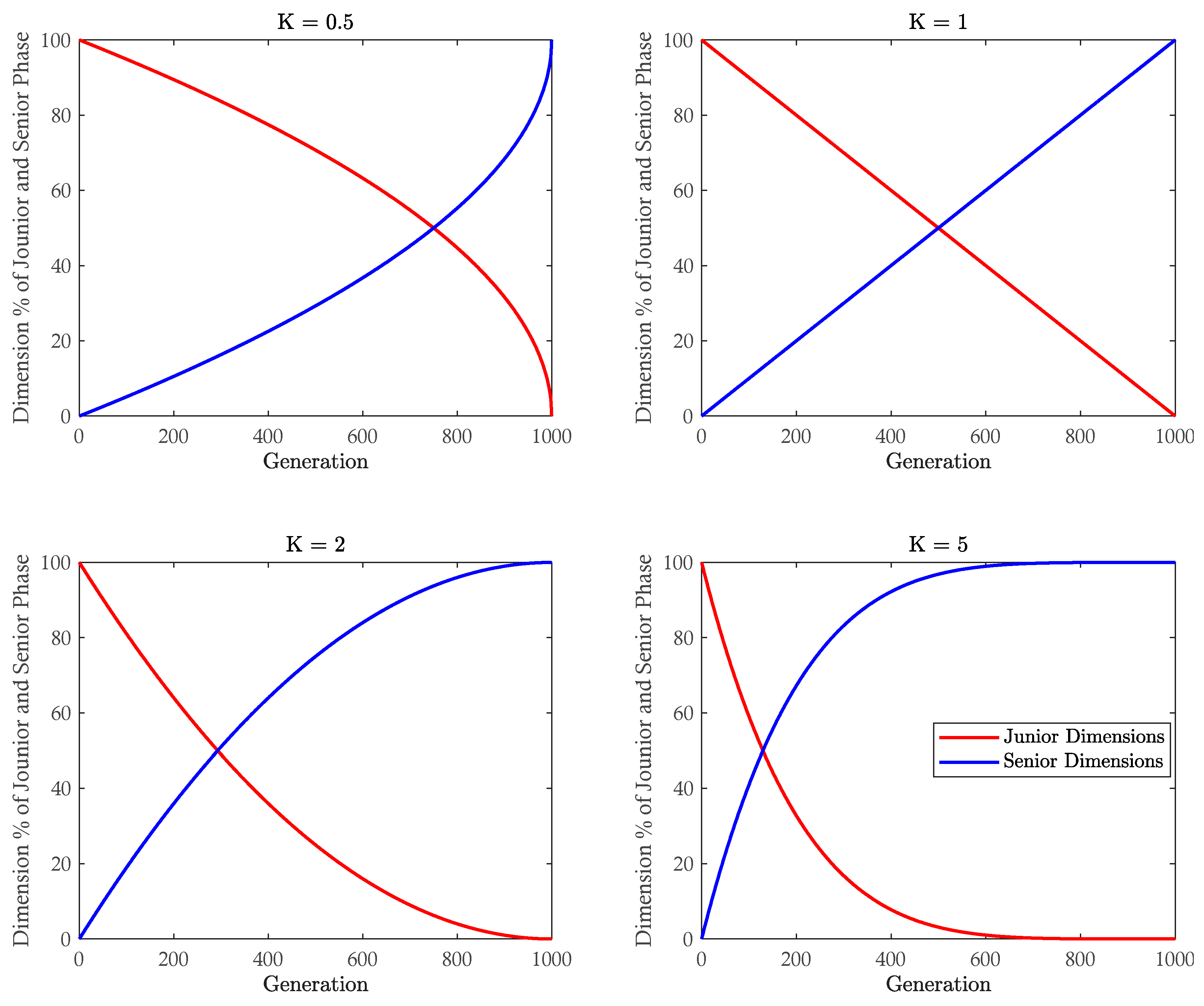
| K | G | D (Junior) | D (Senior) |
|---|---|---|---|
| 0.5 | 0 | 100 | 0 |
| 0.25 MaxGen | 87 | 13 | |
| 0.5 MaxGen | 71 | 29 | |
| 0.75 MaxGen | 50 | 50 | |
| MaxGen | 0 | 100 | |
| 1 | 0 | 100 | 0 |
| 0.25 MaxGen | 75 | 25 | |
| 0.5 MaxGen | 50 | 50 | |
| 0.75 MaxGen | 25 | 75 | |
| MaxGen | 0 | 100 | |
| 2 | 0 | 100 | 0 |
| 0.25 MaxGen | 56 | 44 | |
| 0.5 MaxGen | 25 | 75 | |
| 0.75 MaxGen | 6 | 94 | |
| MaxGen | 0 | 100 | |
| 5 | 0 | 100 | 0 |
| 0.25 MaxGen | 24 | 76 | |
| 0.5 MaxGen | 3 | 97 | |
| 0.75 MaxGen | 1 | 99 | |
| MaxGen | 0 | 100 |
| Function | GSK [16] | ATMALS-GSK (Proposed) | ||||||||
|---|---|---|---|---|---|---|---|---|---|---|
| Best | Median | Worst | Mean | STD | Best | Median | Worst | Mean | STD | |
| 1 | 0.00 | 1.85 × 10⁻²¹ | 1.49 × 101 | 3.28 | 5.21 | 0.14 × 10⁻³ | 1.01 × 101 | 1.54 × 101 | 6.63 | 6.10 |
| 2 | −1.35 × 101 | −1.14 × 101 | −9.25 | −1.13 × 101 | 1.03 | −2.40 × 101 | −1.69 × 101 | −1.19 × 101 | −1.76 × 101 | 3.13 |
| 3 | 1.15 × 10⁻⁵ | 1.15 × 10⁻⁵ | 1.15 × 10⁻⁵ | 1.15 × 10⁻⁵ | 9.12 × 10⁻¹³ | 1.15 × 10⁻⁵ | 1.15 × 10⁻⁵ | 1.15 × 10⁻⁵ | 1.15 × 10⁻⁵ | 1.13× 10⁻²⁰ |
| 4 | 0.00 | 0.00 | 0.00 | 0.00 | 0.00 | 0.00 | 0.00 | 0.00 | 0.00 | 0.00 |
| 5 | −2.39 × 101 | −2.08 × 101 | −1.87 × 101 | −2.06 × 101 | 1.21 | −3.59 × 101 | −2.89 × 101 | −2.42 × 101 | −2.97 × 101 | 3.31 |
| 6 | −1.16 × 101 | −6.85 | 0.00 | −6.94 | 2.48 | −2.91 × 101 | −1.85 × 101 | −7.69 | −1.79 × 101 | 4.85 |
| 7 | 1.59 | 1.78 | 1.97 | 1.78 | 1.08 × 10⁻¹ | 9.99 × 10⁻¹ | 1.2 | 1.49 | 1.29 | 1.25 × 10⁻¹ |
| 8 | 2.20 × 10² | 2.20 × 10² | 2.20 × 10² | 2.20 × 10² | 0.00 | 2.20 × 10² | 2.20 × 10² | 2.20 × 10² | 2.20 × 10² | 0.00 |
| 9 | 1.29 × 10³ | 2.07 × 10³ | 3.09 × 10³ | 2.11 × 10³ | 5.02 × 10² | 1.52 × 10³ | 2.43 × 10³ | 5.31 × 10³ | 2.67 × 10³ | 9.43 × 10² |
| 10 | −2.18 × 101 | −2.16 × 101 | −2.14 × 101 | −2.16 × 101 | 1.19 × 10⁻¹ | −2.18 × 101 | −1.75 × 101 | −1.30 × 101 | −1.81 × 101 | 3.07 |
| 11 | 5.09 × 10⁴ | 5.24 × 10⁴ | 5.39 × 10⁴ | 5.24 × 10⁴ | 6.88 × 10² | 5.15 × 10⁴ | 5.23 × 10⁴ | 5.31 × 10⁴ | 5.23 × 10⁴ | 4.29 × 10² |
| 12 | 1.07 × 10⁶ | 1.07 × 10⁶ | 1.08 × 10⁶ | 1.07 × 10⁶ | 1.73 × 10³ | 1.06 × 10⁶ | 1.07 × 10⁶ | 1.07 × 10⁶ | 1.07 × 10⁶ | 2.10 × 10³ |
| 13 | 1.54 × 10⁴ | 1.54 × 10⁴ | 1.55 × 10⁴ | 1.54 × 10⁴ | 2.44 | 1.54 × 10⁴ | 1.54 × 10⁴ | 1.54 × 10⁴ | 1.54 × 10⁴ | 1.29 × 10⁻⁵ |
| 14 | 1.82 × 10⁴ | 1.84 × 10⁴ | 1.86 × 10⁴ | 1.84 × 10⁴ | 1.22 × 10² | 1.80 × 10⁴ | 1.81 × 10⁴ | 1.84 × 10⁴ | 1.82 × 10⁴ | 1.02 × 10² |
| 15 | 3.28 × 10⁴ | 3.28 × 10⁴ | 3.28 × 10⁴ | 3.28 × 10⁴ | 1.55 × 101 | 3.27 × 10⁴ | 3.27 × 10⁴ | 3.28 × 10⁴ | 3.27 × 10⁴ | 3.13 × 101 |
| 16 | 1.32 × 10⁵ | 1.35 × 10⁵ | 1.39 × 10⁵ | 1.35 × 10⁵ | 2.22 × 10³ | 1.25 × 10⁵ | 1.27 × 10⁵ | 1.29 × 10⁵ | 1.27 × 10⁵ | 9.35 × 10² |
| 17 | 1.97 × 10⁶ | 2.03 × 10⁶ | 2.36 × 10⁶ | 2.09 × 10⁶ | 1.20 × 10⁵ | 1.87 × 10⁶ | 1.89 × 10⁶ | 1.93 × 10⁶ | 1.90 × 10⁶ | 1.61 × 10⁴ |
| 18 | 1.17 × 10⁶ | 1.27 × 10⁶ | 1.57 × 10⁶ | 1.27 × 10⁶ | 7.56 × 10⁴ | 9.36 × 10⁵ | 9.42 × 10⁵ | 9.46 × 10⁵ | 9.42 × 10⁵ | 2476.651 |
| 19 | 1.75 × 10⁶ | 2.03 × 10⁶ | 2.25 × 10⁶ | 2.00 × 10⁶ | 1.36 × 10⁵ | 9.37 × 10⁵ | 9.47 × 10⁵ | 9.76 × 10⁵ | 9.47 × 10⁵ | 7.47 × 10³ |
| 20 | 1.12 × 10⁶ | 1.29 × 10⁶ | 1.46 × 10⁶ | 1.29 × 10⁶ | 9.20 × 10⁴ | 9.35 × 10⁵ | 9.41 × 10⁵ | 9.47 × 10⁵ | 9.41 × 10⁵ | 3.28 × 10³ |
| 21 | 1.34 × 101 | 1.61 × 101 | 2.49 × 101 | 1.70 × 101 | 3.11 | 1.52 × 101 | 1.95 × 101 | 2.40 × 101 | 1.92 × 101 | 2.11 |
| 22 | 8.61 | 1.28 × 101 | 2.09 × 101 | 1.29 × 101 | 2.93 | 8.61 | 1.63 × 101 | 2.39 × 101 | 1.61 × 101 | 3.97 |
| Algorithms | R+ | R− | p Value | + | = | − | Dec. |
|---|---|---|---|---|---|---|---|
| ATMALS−GSK vs. GSK | 127 | 26 | 0.0168 | 12 | 5 | 5 | + |
| Function | GSK [16] | ATMALS-GSK (Proposed) | ||||||||
|---|---|---|---|---|---|---|---|---|---|---|
| Best | Median | Worst | Mean | STD | Best | Median | Worst | Mean | STD | |
| 1 | 0.00 | 0.00 | 0.00 | 0.00 | 0.00 | 0.00 | 0.00 | 0.00 | 0.00 | 0.00 |
| 3 | 0.00 | 0.00 | 0.00 | 0.00 | 0.00 | 0.00 | 0.00 | 0.00 | 0.00 | 0.00 |
| 4 | 0.00 | 0.00 | 0.00 | 0.00 | 0.00 | 0.00 | 0.00 | 0.00 | 0.00 | 0.00 |
| 5 | 1.53 × 101 | 2.01 × 101 | 2.58 × 101 | 2.03 × 101 | 2.79 | 2.99 | 8.47 | 1.00 × 101 | 7.57 | 2.71 |
| 6 | 0.00 | 0.00 | 0.00 | 0.00 | 0.00 | 0.00 | 0.00 | 0.00 | 0.00 | 0.00 |
| 7 | 2.46 × 101 | 3.10 × 101 | 3.74 × 101 | 3.07 × 101 | 3.08 | 1.27 × 101 | 1.69 × 101 | 1.85 × 101 | 1.63 × 101 | 2.21 |
| 8 | 1.45 × 101 | 1.99 × 101 | 2.58 × 101 | 2.02 × 101 | 2.92 | 3.98 | 7.97 | 1.09 × 101 | 7.57 | 2.11 |
| 9 | 0.00 | 0.00 | 0.00 | 0.00 | 0.00 | 0.00 | 0.00 | 0.00 | 0.00 | 0.00 |
| 10 | 7.54 × 10² | 1.10 × 10³ | 1.29 × 10³ | 1.06 × 10³ | 1.33 × 10² | 1.40 × 10² | 5.07 × 10² | 6.57 × 10² | 4.55 × 10² | 1.93 × 10² |
| 11 | 0.00 | 0.00 | 1.02× 10⁻⁸ | 0.00 | 0.00 | 6.40 × 10⁻¹ | 1.77 | 2.67 | 1.67 | 7.10 × 10⁻¹ |
| 12 | 1.42 × 101 | 7.57 × 101 | 2.69 × 10² | 8.93 × 101 | 7.26 × 101 | 2.12 × 10⁻¹ | 1.05 × 101 | 3.45 × 101 | 1.12 × 101 | 9.45 |
| 13 | 9.19 × 10⁻¹ | 6.56 | 9.73 | 6.56 | 1.41 | 3.32 × 10⁻¹ | 1.80 | 5.70 | 2.65 | 2.18 |
| 14 | 5.19 × 10⁻³ | 5.42 | 1.19 × 101 | 5.88 | 3.06 | 3.57 × 10⁻¹ | 2.94 | 3.56 | 2.78 | 9.25 × 10⁻¹ |
| 15 | 2.96 × 10⁻³ | 1.75 × 10⁻¹ | 5.00 × 10⁻¹ | 2.22 × 10⁻¹ | 2.13 × 10⁻¹ | 1.45 × 10⁻² | 1.30 × 10⁻¹ | 2.63 × 10⁻¹ | 1.47 × 10⁻¹ | 8.60 × 10⁻² |
| 16 | 3.29 × 10⁻¹ | 9.48 × 10⁻¹ | 1.18 × 101 | 4.27 | 4.95 | 4.89 × 10⁻¹ | 1.11 | 1.80 | 1.12 | 4.70 × 10⁻¹ |
| 17 | 9.76 × 10⁻¹ | 9.94 | 2.52 × 101 | 1.17 × 101 | 7.09 | 2.26 | 1.26 × 101 | 2.27 × 101 | 1.25 × 101 | 9.02 × 101 |
| 18 | 2.05 × 10⁻² | 4.30 × 10⁻¹ | 5.01 × 10⁻¹ | 3.20 × 10⁻¹ | 1.92 × 10⁻¹ | 3.94 × 10⁻² | 3.32 × 10⁻¹ | 4.95 × 10⁻¹ | 3.04 × 10⁻¹ | 1.85 × 10⁻¹ |
| 19 | 2.81 × 10⁻² | 6.95 × 10⁻² | 1.80 | 1.55 × 10⁻¹ | 3.51 × 10⁻¹ | 5.36 × 10⁻² | 1.27 × 10⁻¹ | 2.20 × 10⁻¹ | 1.39 × 10⁻¹ | 5.66 × 10⁻² |
| 20 | 3.12 × 10⁻¹ | 3.12 × 10⁻¹ | 2.03 × 101 | 1.19 | 3.99 | 1.16 | 1.97 | 4.55 | 2.51 | 1.14 |
| 21 | 1.00 × 10² | 2.20 × 10² | 2.31 × 10² | 1.93 × 10² | 5.07 × 101 | 1.00 × 10² | 1.00 × 10² | 1.00 × 10² | 1.00 × 10² | 0.00 |
| 22 | 1.00 × 10² | 1.00 × 10² | 1.02 × 10² | 1.00 × 10² | 4.87 × 10⁻¹ | 0.00 | 1.00 × 10² | 1.00 × 10² | 6.38 × 101 | 4.73 × 101 |
| 23 | 3.11 × 10² | 3.18 × 10² | 3.29 × 10² | 3.18 × 10² | 3.99 | 2.24 × 10⁻¹ | 3.06 × 10² | 3.10 × 10² | 2.76 × 10² | 9.72 × 101 |
| 24 | 2.78 × 10² | 3.50 × 10² | 3.57 × 10² | 3.44 × 10² | 1.87 × 101 | 1.00 × 10² | 3.35 × 10² | 3.39 × 10² | 3.11 × 10² | 7.44 × 101 |
| 25 | 3.98 × 10² | 4.34 × 10² | 4.46 × 10² | 4.27 × 10² | 2.05 × 101 | 3.97 × 10² | 3.97 × 10² | 3.98 × 10² | 3.97 × 10² | 1.32 × 10⁻¹ |
| 26 | 3.00 × 10² | 3.00 × 10² | 3.00 × 10² | 3.00 × 10² | 0.00 | 3.00 × 10² | 3.00 × 10² | 3.00 × 10² | 3.00 × 10² | 0.00 |
| 27 | 3.89 × 10² | 3.90 × 10² | 3.90 × 10² | 3.89 × 10² | 2.17 × 10⁻¹ | 3.89 × 10² | 3.89 × 10² | 3.89 × 10² | 3.89 × 10² | 1.98 × 10⁻¹ |
| 28 | 3.00 × 10² | 3.00 × 10² | 3.97 × 10² | 3.12 × 10² | 3.20 × 101 | 3.00 × 10² | 3.00 × 10² | 3.00 × 10² | 3.00 × 10² | 0.00 |
| 29 | 2.39 × 10² | 2.48 × 10² | 2.57 × 10² | 2.48 × 10² | 4.76 | 2.32 × 10² | 2.39 × 10² | 2.43 × 10² | 2.38 × 10² | 3.33 |
| 30 | 3.96 × 10² | 4.65 × 10² | 5.02 × 10² | 4.56 × 10² | 3.44 × 101 | 3.94 × 10² | 4.42 × 10² | 4.42 × 10² | 4.29 × 10² | 2.09 × 101 |
| Function | GSK [16] | ATMALS-GSK (Proposed) | ||||||||
|---|---|---|---|---|---|---|---|---|---|---|
| Best | Median | Worst | Mean | STD | Best | Median | Worst | Mean | STD | |
| 1 | 0.00 | 0.00 | 0.00 | 0.00 | 0.00 | 0.00 | 0.00 | 0.00 | 0.00 | 0.00 |
| 3 | 0.00 | 5.66 × 10⁻⁸ | 8.54 × 10⁻⁶ | 7.07 × 10⁻⁷ | 1.82 × 10⁻⁶ | 0.00 | 0.00 | 0.00 | 0.00 | 0.00 |
| 4 | 9.28 × 10⁻³ | 4.00 | 7.25 × 101 | 1.11 × 101 | 2.17 × 101 | 0.00 | 1.99 | 3.98 | 1.99 | 2.10 |
| 5 | 1.36 × 10² | 1.62 × 10² | 1.73 × 10² | 1.60 × 10² | 8.87 | 1.08 × 101 | 2.67 × 101 | 9.72 × 101 | 1.53 × 101 | 1.90 × 101 |
| 6 | 0.00 | 5.47 × 10⁻⁷ | 8.42 × 10⁻⁶ | 1.52 × 10⁻⁶ | 2.36 × 10⁻⁶ | 2.26 × 10⁻⁵ | 5.71 × 10⁻⁵ | 1.39 × 10⁻⁴ | 6.82 × 10⁻⁵ | 3.90 × 10⁻⁵ |
| 7 | 1.64 × 10² | 1.87 × 10² | 1.99 × 10² | 1.87 × 10² | 8.40 | 2.52 × 101 | 5.60 × 101 | 9.83 × 101 | 4.33 × 101 | 1.15 × 101 |
| 8 | 1.24 × 10² | 1.56 × 10² | 1.73 × 10² | 1.55 × 10² | 1.11 × 101 | 1.07 × 101 | 2.34 × 101 | 5.06 × 101 | 1.35 × 101 | 1.29 × 101 |
| 9 | 0.00 | 0.00 | 0.00 | 0.00 | 0.00 | 0.00 | 0.00 | 8.95 × 10⁻² | 1.79 × 10⁻² | 3.77 × 10⁻² |
| 10 | 5.84 × 10³ | 6.68 × 10³ | 7.16 × 10³ | 6.69 × 10³ | 3.54 × 10² | 1.63 × 10³ | 2.96 × 10³ | 3.49 × 10³ | 2.80 × 10³ | 5.90 × 10² |
| 11 | 6.00 × 10⁻¹ | 8.57 | 9.85 × 101 | 3.30 × 101 | 3.83 × 101 | 9.94 | 2.04 × 101 | 7.19 × 101 | 1.46 × 101 | 1.73 × 101 |
| 12 | 1.03 × 10³ | 5.32 × 10³ | 1.91 × 10⁴ | 6.62 × 10³ | 4.59 × 10³ | 9.02 × 10² | 3.12 × 10³ | 8.19 × 10³ | 3.84 × 10³ | 2.62 × 10³ |
| 13 | 4.61 × 101 | 9.11 × 101 | 1.82 × 10² | 9.83 × 101 | 3.42 × 101 | 2.06 × 101 | 3.91 × 101 | 6.34 × 101 | 3.01 × 101 | 1.12 × 101 |
| 14 | 4.72 × 101 | 5.73 × 101 | 6.65 × 101 | 5.69 × 101 | 5.49 | 1.04 × 101 | 1.79 × 101 | 4.57 × 101 | 1.78 × 101 | 4.26 |
| 15 | 2.13 | 9.17 | 7.48 × 101 | 1.45 × 101 | 1.49 × 101 | 5.88 | 1.75 × 101 | 1.92 × 101 | 1.43 × 101 | 5.56 |
| 16 | 4.35 × 10² | 7.76 × 10² | 1.15 × 10³ | 7.96 × 10² | 1.94 × 10² | 1.97 × 101 | 5.47 × 10² | 7.50 × 10² | 2.53 × 10² | 2.81 × 10² |
| 17 | 6.28 × 101 | 2.04 × 10² | 3.77 × 10² | 1.89 × 10² | 9.44 × 101 | 2.92 × 101 | 6.37 × 101 | 1.41 × 10² | 4.71 × 101 | 2.30 × 101 |
| 18 | 2.25 × 101 | 3.69 × 101 | 4.80 × 101 | 3.68 × 101 | 5.42 | 2.25 × 101 | 2.74 × 101 | 4.02 × 101 | 3.02 × 101 | 6.67 |
| 19 | 3.42 | 1.13 × 101 | 2.22 × 101 | 1.29 × 101 | 6.02 | 8.03 | 1.37 × 101 | 1.65 × 101 | 1.30 × 101 | 3.34 |
| 20 | 1.34 | 5.51 × 101 | 4.51 × 10² | 1.08 × 10² | 1.14 × 10² | 3.73 × 101 | 5.58 × 101 | 1.62 × 10² | 4.74 × 101 | 3.35 × 101 |
| 21 | 3.20 × 10² | 3.49 × 10² | 3.55 × 10² | 3.46 × 10² | 8.30 | 2.51 × 10² | 2.65 × 10² | 2.79 × 10² | 2.66 × 10² | 9.12 |
| 22 | 1.00 × 10² | 1.00 × 10² | 1.00 × 10² | 1.00 × 10² | 0.00 | 1.00 × 10² | 1.00 × 10² | 1.00 × 10² | 1.00 × 10² | 0.00 |
| 23 | 3.50 × 10² | 4.86 × 10² | 5.07 × 10² | 4.70 × 10² | 4.49 × 101 | 3.97 × 10² | 4.28 × 10² | 4.43 × 10² | 3.44 × 10² | 1.70 × 101 |
| 24 | 5.29 × 10² | 5.70 × 10² | 5.86 × 10² | 5.68 × 10² | 1.45 × 101 | 4.52 × 10² | 4.77 × 10² | 4.91 × 10² | 4.75 × 10² | 1.48 × 101 |
| 25 | 3.87 × 10² | 3.87 × 10² | 3.87 × 10² | 3.87 × 10² | 2.11 × 10⁻¹ | 3.83 × 10² | 3.86 × 10² | 3.87 × 10² | 3.86 × 10² | 1.07 |
| 26 | 6.93 × 10² | 9.56 × 10² | 2.12 × 10³ | 9.87 × 10² | 2.49 × 10² | 1.45 × 10³ | 1.87 × 10³ | 1.97 × 10³ | 1.79 × 10³ | 1.93 × 10² |
| 27 | 4.80 × 10² | 4.92 × 10² | 5.14 × 10² | 4.93 × 10² | 8.02 | 4.87 × 10² | 4.97 × 10² | 5.06 × 10² | 4.96 × 10² | 6.31 |
| 28 | 3.00 × 10² | 3.00 × 10² | 4.04 × 10² | 3.21 × 10² | 4.22 × 101 | 3.00 × 10² | 3.00 × 10² | 4.03 × 10² | 3.10 × 10² | 3.26 × 101 |
| 29 | 4.23 × 10² | 5.92 × 10² | 7.69 × 10² | 5.77 × 10² | 1.01 × 10² | 4.09 × 10² | 5.13 × 10² | 5.68 × 10² | 4.32 × 10² | 5.95 × 101 |
| 30 | 1.94 × 10³ | 2.09 × 10³ | 2.36 × 10³ | 2.08 × 10³ | 9.27 × 101 | 1.97 × 10³ | 2.06 × 10³ | 2.12 × 10³ | 2.06 × 10³ | 5.55 × 101 |
| Function | GSK [16] | ATMALS-GSK (Proposed) | ||||||||
|---|---|---|---|---|---|---|---|---|---|---|
| Best | Median | Worst | Mean | STD | Best | Median | Worst | Mean | STD | |
| 1 | 1.71 × 101 | 4.73 × 10² | 4.61 × 10³ | 1.09 × 10³ | 1.24 × 10³ | 9.10 × 10⁻⁴ | 1.25 × 10⁻¹ | 3.41 × 10⁻¹ | 1.25 × 10⁻¹ | 2.15 × 10⁻¹ |
| 3 | 1.61 × 10³ | 3.79 × 10³ | 6.73 × 10³ | 3.85 × 10³ | 1.51 × 10³ | 1.12 × 10² | 7.85 × 10² | 1.46 × 10³ | 7.85 × 10² | 6.73 × 10² |
| 4 | 1.33 × 10⁻² | 7.21 × 101 | 1.46 × 10² | 8.33 × 101 | 5.00 × 101 | 8.20 | 9.80 | 2.70 × 101 | 9.80 | 1.82 × 101 |
| 5 | 2.65 × 10² | 3.25 × 10² | 3.45 × 10² | 3.20 × 10² | 1.79 × 101 | 2.98 × 101 | 4.21 × 101 | 9.48 × 101 | 3.21 × 101 | 1.27 × 101 |
| 6 | 3.11 × 10⁻⁷ | 2.80 × 10⁻⁶ | 1.64 × 10⁻⁵ | 3.78 × 10⁻⁶ | 3.52 × 10⁻⁶ | 1.17 × 10⁻⁷ | 7.14 × 10⁻⁶ | 1.55 × 10⁻⁵ | 7.14 × 10⁻⁶ | 8.31 × 10⁻⁶ |
| 7 | 3.29 × 10² | 3.74 × 10² | 3.86 × 10² | 3.70 × 10² | 1.41 × 101 | 9.68 × 101 | 1.08 × 10² | 1.19 × 10² | 1.08 × 10² | 1.12 × 101 |
| 8 | 2.90 × 10² | 3.28 × 10² | 3.38 × 10² | 3.24 × 10² | 1.36 × 101 | 5.16 × 101 | 6.15 × 101 | 7.14 × 101 | 3.85 × 101 | 9.92 |
| 9 | 0.00 | 0.00 | 8.95 × 10⁻² | 1.07 × 10⁻² | 2.79 × 10⁻² | 1.50 × 10⁻² | 1.91 × 10⁻¹ | 3.97 × 10⁻¹ | 1.91 × 10⁻¹ | 2.06 × 10⁻¹ |
| 10 | 1.21 × 10⁴ | 1.28 × 10⁴ | 1.37 × 10⁴ | 1.30 × 10⁴ | 4.50 × 10² | 7.88 × 10³ | 8.80 × 10³ | 9.73 × 10³ | 8.80 × 10³ | 9.25 × 10² |
| 11 | 2.34 × 101 | 2.96 × 101 | 1.45 × 10² | 3.45 × 101 | 2.32 × 101 | 2.59 × 101 | 3.11 × 101 | 3.63 × 101 | 2.91 × 101 | 5.17 |
| 12 | 2.16 × 10³ | 7.71 × 10³ | 3.17 × 10⁴ | 9.46 × 10³ | 7.01 × 10³ | 1.53 × 10⁴ | 3.65 × 10⁴ | 5.77 × 10⁴ | 3.65 × 10⁴ | 2.12 × 10⁴ |
| 13 | 7.41 × 101 | 6.24 × 10² | 8.98 × 10³ | 1.49 × 10³ | 2.16 × 10³ | 6.72 × 101 | 1.19 × 10² | 1.71 × 10² | 1.19 × 10² | 5.17 × 101 |
| 14 | 5.76 × 101 | 1.28 × 10² | 1.42 × 10² | 1.24 × 10² | 1.87 × 101 | 2.77 × 101 | 3.69 × 101 | 4.60 × 101 | 3.69 × 101 | 9.02 |
| 15 | 2.52 × 101 | 3.62 × 101 | 1.00 × 10² | 4.20 × 101 | 1.68 × 101 | 3.31 × 101 | 4.45 × 101 | 5.59 × 101 | 4.45 × 101 | 1.14 × 101 |
| 16 | 1.30 × 10² | 2.01 × 10³ | 2.70 × 10³ | 1.83 × 10³ | 6.59 × 10² | 4.56 × 10² | 7.91 × 10² | 1.13 × 10³ | 4.91 × 10² | 3.35 × 10² |
| 17 | 7.75 × 10² | 1.39 × 10³ | 1.63 × 10³ | 1.35 × 10³ | 1.90 × 10² | 4.77 × 10² | 7.08 × 10² | 9.39 × 10² | 7.08 × 10² | 2.31 × 10² |
| 18 | 1.78 × 10² | 5.01 × 10² | 1.45 × 10³ | 5.98 × 10² | 3.37 × 10² | 4.40 × 101 | 1.17 × 10² | 1.90 × 10² | 1.17 × 10² | 7.30 × 101 |
| 19 | 1.84 × 101 | 2.92 × 101 | 5.13 × 101 | 3.05 × 101 | 9.59 | 2.05 × 101 | 2.83 × 101 | 3.62 × 101 | 2.83 × 101 | 7.93 |
| 20 | 1.17 × 10³ | 1.40 × 10³ | 1.62 × 10³ | 1.37 × 10³ | 1.28 × 10² | 5.44 × 10² | 6.91 × 10² | 8.38 × 10² | 6.91 × 10² | 1.48 × 10² |
| 21 | 4.90 × 10² | 5.25 × 10² | 5.46 × 10² | 5.21 × 10² | 1.31 × 101 | 1.91 × 10² | 1.98 × 10² | 2.05 × 10² | 1.98 × 10² | 6.81 |
| 22 | 1.00 × 10² | 1.31 × 10⁴ | 1.35 × 10⁴ | 1.10 × 10⁴ | 4.85 × 10³ | 6.29 × 10³ | 8.71 × 10³ | 1.11 × 10⁴ | 8.71 × 10³ | 2.41 × 10³ |
| 23 | 4.20 × 10² | 4.46 × 10² | 7.49 × 10² | 5.42 × 10² | 1.39 × 10² | 4.66 × 10² | 4.79 × 10² | 4.92 × 10² | 4.39 × 10² | 1.27 × 101 |
| 24 | 5.01 × 10² | 5.24 × 10² | 8.11 × 10² | 6.34 × 10² | 1.39 × 10² | 5.41 × 10² | 5.54 × 10² | 5.68 × 10² | 5.14 × 10² | 1.35 × 101 |
| 25 | 4.60 × 10² | 5.64 × 10² | 6.11 × 10² | 5.56 × 10² | 4.62 × 101 | 5.18 × 10² | 5.45 × 10² | 5.72 × 10² | 5.45 × 10² | 2.74 × 101 |
| 26 | 1.06 × 10³ | 1.29 × 10³ | 1.42 × 10³ | 1.27 × 10³ | 9.18 × 101 | 9.95 × 10² | 1.35 × 10³ | 1.71 × 10³ | 1.35 × 10³ | 3.55 × 10² |
| 27 | 5.18 × 10² | 5.64 × 10² | 9.16 × 10² | 5.92 × 10² | 8.29 × 101 | 5.43 × 10² | 5.71 × 10² | 5.99 × 10² | 5.71 × 10² | 2.78 × 101 |
| 28 | 4.59 × 10² | 4.97 × 10² | 5.70 × 10² | 4.94 × 10² | 2.24 × 101 | 4.64 × 10² | 4.88 × 10² | 5.12 × 10² | 4.88 × 10² | 2.39 × 101 |
| 29 | 3.28 × 10² | 3.55 × 10² | 4.09 × 10² | 3.60 × 10² | 2.23 × 101 | 4.59 × 10² | 5.01 × 10² | 5.43 × 10² | 5.01 × 10² | 4.19 × 101 |
| 30 | 5.79 × 10⁵ | 5.81 × 10⁵ | 6.52 × 10⁵ | 5.96 × 10⁵ | 2.24 × 10⁴ | 5.74 × 10⁵ | 5.92 × 10⁵ | 6.11 × 10⁵ | 5.92 × 10⁵ | 1.85 × 10⁴ |
| Function | GSK [16] | ATMALS-GSK (Proposed) | ||||||||
|---|---|---|---|---|---|---|---|---|---|---|
| Best | Median | Worst | Mean | STD | Best | Median | Worst | Mean | STD | |
| 1 | 3.96 × 10⁻¹ | 5.38 × 10³ | 2.11 × 10⁴ | 5.80 × 10³ | 4.63 × 10³ | 1.96 × 10⁻¹ | 1.98 | 7.98 | 2.55 | 4.79 |
| 3 | 6.01 × 10⁴ | 1.15 × 10⁵ | 1.48 × 10⁵ | 1.15 × 10⁵ | 2.15 × 10⁴ | 4.87 × 10⁴ | 4.91 × 10⁴ | 5.30 × 10⁴ | 4.91 × 10⁴ | 1.26 × 10⁴ |
| 4 | 8.46 × 101 | 2.17 × 10² | 2.89 × 10² | 2.05 × 10² | 4.57 × 101 | 1.81 × 10² | 1.97 × 10² | 2.03 × 10² | 1.98 × 10² | 1.45 × 101 |
| 5 | 7.26 × 101 | 7.70 × 10² | 8.14 × 10² | 5.31 × 10² | 3.39 × 10² | 3.70 × 10² | 5.30 × 10² | 5.90 × 10² | 5.40 × 10² | 2.17 × 101 |
| 6 | 1.25 × 10⁻⁵ | 6.83 × 10⁻⁵ | 3.14 × 10⁻² | 1.72 × 10⁻³ | 6.46 × 10⁻³ | 1.80 × 10⁻⁶ | 6.20 × 10⁻³ | 3.90 × 10⁻² | 1.24 × 10⁻² | 2.73 × 10⁻² |
| 7 | 8.33 × 10² | 8.76 × 10² | 9.16 × 10² | 8.75 × 10² | 1.83 × 101 | 6.99 × 10² | 8.21 × 10² | 8.99 × 10² | 8.20 × 10² | 1.91 × 101 |
| 8 | 5.90 × 101 | 7.36 × 10² | 8.18 × 10² | 4.92 × 10² | 3.41 × 10² | 3.95 × 10² | 4.91 × 10² | 5.88 × 10² | 4.92 × 10² | 1.12 × 101 |
| 9 | 5.45 | 7.69 | 1.72 × 101 | 8.46 | 3.41 | 4.75 | 8.90 | 1.60 × 101 | 8.80 | 3.14 |
| 10 | 2.87 × 10⁴ | 2.94 × 10⁴ | 3.04 × 10⁴ | 2.95 × 10⁴ | 4.44 × 10² | 2.28 × 10⁴ | 2.45 × 10⁴ | 2.85 × 10⁴ | 2.44 × 10⁴ | 1.01 × 10³ |
| 11 | 1.61 × 10² | 2.65 × 10² | 4.64 × 10² | 2.78 × 10² | 6.85 × 101 | 1.30 × 10² | 1.70 × 10² | 2.80 × 10² | 1.76 × 10² | 6.28 × 101 |
| 12 | 2.25 × 10⁴ | 6.53 × 10⁴ | 3.23 × 10⁵ | 8.34 × 10⁴ | 7.52 × 10⁴ | 1.20 × 10⁴ | 2.92 × 10⁵ | 5.88 × 10⁵ | 3.78 × 10⁵ | 1.69 × 10⁵ |
| 13 | 5.17 × 101 | 2.85 × 10³ | 9.31 × 10³ | 3.20 × 10³ | 2.64 × 10³ | 1.06 × 10² | 1.30 × 10² | 2.00 × 10² | 1.31 × 10² | 5.43 × 101 |
| 14 | 3.30 × 10² | 2.53 × 10³ | 1.69 × 10⁴ | 4.64 × 10³ | 4.47 × 10³ | 6.20 × 10² | 2.49 × 10³ | 3.50 × 10³ | 2.57 × 10³ | 2.31 × 10³ |
| 15 | 3.20 × 101 | 4.23 × 10² | 5.20 × 10³ | 7.33 × 10² | 1.09 × 10³ | 5.90 × 101 | 9.90 × 101 | 1.40 × 10² | 1.04 × 10² | 4.05 × 101 |
| 16 | 2.87 × 10² | 8.25 × 10² | 7.04 × 10³ | 2.27 × 10³ | 2.61 × 10³ | 8.60 × 10² | 1.80 × 10³ | 2.30 × 10³ | 1.89 × 10³ | 4.24 × 10² |
| 17 | 2.14 × 10³ | 4.12 × 10³ | 4.59 × 10³ | 3.91 × 10³ | 6.68 × 10² | 8.00 × 10² | 1.30 × 10³ | 2.80 × 10³ | 1.57 × 10³ | 6.92 × 10² |
| 18 | 1.93 × 10⁴ | 4.43 × 10⁴ | 1.87 × 10⁵ | 5.73 × 10⁴ | 3.63 × 10⁴ | 9.50 × 10³ | 1.13 × 10⁴ | 1.30 × 10⁴ | 1.14 × 10⁴ | 4.25 × 10³ |
| 19 | 5.04 × 101 | 8.41 × 10² | 3.25 × 10³ | 1.00 × 10³ | 8.30 × 10² | 9.00 × 101 | 1.55 × 10² | 2.30 × 10² | 1.61 × 10² | 7.63 × 101 |
| 20 | 3.97 × 10³ | 4.52 × 10³ | 4.80 × 10³ | 4.46 × 10³ | 2.22 × 10² | 3.10 × 10³ | 2.80 × 10³ | 2.90 × 10³ | 2.84 × 10³ | 5.21 × 10² |
| 21 | 2.83 × 10² | 3.29 × 10² | 1.02 × 10³ | 6.07 × 10² | 3.37 × 10² | 2.10 × 10² | 2.85 × 10² | 3.10 × 10² | 2.89 × 10² | 2.11 × 101 |
| 22 | 2.86 × 10⁴ | 3.01 × 10⁴ | 3.09 × 10⁴ | 3.00 × 10⁴ | 4.57 × 10² | 2.10 × 10⁴ | 2.35 × 10⁴ | 3.80 × 10⁴ | 2.43 × 10⁴ | 1.92 × 10³ |
| 23 | 5.86 × 10² | 6.11 × 10² | 6.49 × 10² | 6.11 × 10² | 1.58 × 101 | 5.25 × 10² | 5.85 × 10² | 6.45 × 10² | 5.87 × 10² | 1.45 × 101 |
| 24 | 8.89 × 10² | 9.33 × 10² | 9.69 × 10² | 9.32 × 10² | 1.70 × 101 | 8.40 × 10² | 9.10 × 10² | 9.50 × 10² | 9.11 × 10² | 1.77 × 101 |
| 25 | 7.61 × 10² | 8.20 × 10² | 8.99 × 10² | 8.21 × 10² | 4.34 × 101 | 7.20 × 10² | 7.50 × 10² | 7.80 × 10² | 7.53 × 10² | 4.18 × 101 |
| 26 | 3.33 × 10³ | 3.63 × 10³ | 3.96 × 10³ | 3.66 × 10³ | 1.78 × 10² | 3.12 × 10³ | 3.35 × 10³ | 3.65 × 10³ | 3.42 × 10³ | 1.28 × 10³ |
| 27 | 6.20 × 10² | 6.46 × 10² | 7.30 × 10² | 6.57 × 10² | 3.07 × 101 | 6.10 × 10² | 6.78 × 10² | 7.90 × 10² | 6.87 × 10² | 3.47 × 101 |
| 28 | 4.99 × 10² | 5.57 × 10² | 6.09 × 10² | 5.53 × 10² | 3.25 × 101 | 3.10 × 10² | 3.30 × 10² | 3.85 × 10² | 3.51 × 10² | 1.10 × 10² |
| 29 | 9.12 × 10² | 1.21 × 10³ | 1.56 × 10³ | 1.21 × 10³ | 1.74 × 10² | 1.01 × 10³ | 1.37 × 10³ | 1.78 × 10³ | 1.39 × 10³ | 2.14 × 10² |
| 30 | 2.41 × 10³ | 3.02 × 10³ | 3.72 × 10³ | 2.99 × 10³ | 2.73 × 10² | 2.40 × 10³ | 3.21 × 10³ | 3.40 × 10³ | 3.23 × 10³ | 8.70 × 10² |
| Fun. | GSK [16] | AGSK [46] | APGSK [45] | FDBAGSK [36] | eGSK [49] | ATMALS-GSK |
|---|---|---|---|---|---|---|
| 1 | 0.00 ± 0.00 | 0.00 ± 0.00 | 0.00 ± 0.00 | 0.00 ± 0.00 | 0.00 ± 0.00 | 0.00 ± 0.00 |
| 3 | 0.00 ± 0.00 | 0.00 ± 0.00 | 0.00 ± 0.00 | 0.00 ± 0.00 | 0.00 ± 0.00 | 0.00 ± 0.00 |
| 4 | 0.00 ± 0.00 | 0.00 ± 0.00 | 0.00 ± 0.00 × 101 | 0.00 ± 0.00 | 0.00 ± 0.00 | 0.00 ± 0.00 |
| 5 | 2.03 × 101 ± 2.79 | 6.33 ± 1.89 | 8.04 ± 2.41 | 5.83 ± 1.64 | 4.82 ± 1.90 | 7.57 ± 2.71 |
| 6 | 0.00 ± 0.00 | 9.52 × 10⁻⁶ ± 2.42 × 10⁻⁵ | 4.45 × 10⁻⁵ ± 1.33 × 10⁻⁴ | 5.59 × 10⁻⁶ ± 1.35 × 10⁻⁵ | 0.00 ± 0.00 | 0.00 ± 0.00 |
| 7 | 3.07 × 101 ± 3.08 | 1.80 × 101 ± 2.39 | 1.90 × 101 ± 3.50 | 1.81 × 101 ± 3.57 | 1.54 × 101 ± 2.43 | 1.63 × 101 ± 2.21 |
| 8 | 2.02 × 101 ± 2.92 | 8.12 ± 2.29 | 9.16 ± 3.07 | 7.54 ± 2.30 | 5.29 ± 2.08 | 7.57 ± 2.11 |
| 9 | 0.00 ± 0.00 | 1.42 × 10⁻² ± 6.64 × 10⁻² | 1.76 × 10⁻³ ± 1.25 × 10⁻² | 0.00 ± 0.00 | 0.00 ± 0.00 | 0.00 ± 0.00 |
| 10 | 1.06 × 10³ ± 1.33 × 10² | 3.20 × 10² ± 8.64 × 101 | 3.05 × 10² ± 1.05 × 10² | 3.02 × 10² ± 1.15 × 10² | 7.59 × 10² ± 2.35 × 10² | 4.55 × 10² ± 1.93 × 10² |
| 11 | 0.00 ± 0.00 | 3.99 × 10⁻¹ ± 8.06 × 10⁻¹ | 1.16 ± 9.76 × 10⁻¹ | 9.30 × 10⁻¹ ± 9.07 × 10⁻¹ | 0.00 ± 0.00 | 1.67 ± 7.10 × 10⁻¹ |
| 12 | 8.93 × 101 ± 7.26 × 101 | 4.46 × 101 ± 5.34 × 101 | 9.50 × 101 ± 8.64 × 101 | 7.06 × 101 ± 5.51 × 101 | 5.58 × 101 ± 6.17 × 101 | 1.12 × 101 ± 9.45 |
| 13 | 6.56 ± 1.41 | 3.35 ± 2.16 | 4.29 ± 2.70 | 4.15 ± 1.96 | 5.50 ± 6.56 × 10⁻¹ | 2.65 ± 2.18 |
| 14 | 5.88 ± 3.06 | 3.91 × 10⁻² ± 1.95 × 10⁻¹ | 5.73 × 10⁻¹ ± 6.10 × 10⁻¹ | 1.41 × 10⁻¹ ± 3.70 × 10⁻¹ | 2.20 × 10⁻¹ ± 4.61 × 10⁻¹ | 2.78 ± 9.25 × 10⁻¹ |
| 15 | 2.22 × 10⁻¹ ± 2.13 × 10⁻¹ | 1.97 × 10⁻² ± 2.88 × 10⁻² | 1.48 × 10⁻¹ ± 2.02 × 10⁻¹ | 3.33 × 10⁻² ± 4.30 × 10⁻² | 3.06 × 10⁻¹ ± 2.18 × 10⁻¹ | 1.47 × 10⁻¹ ± 8.60 × 10⁻² |
| 16 | 4.27 ± 4.95 | 7.01 × 10⁻¹ ± 3.37 × 10⁻¹ | 7.44 × 10⁻¹ ± 7.35 × 10⁻¹ | 1.52 ± 1.01 | 4.37 ± 5.17 | 1.12 ± 4.70 × 10⁻¹ |
| 17 | 1.17 × 101 ± 7.09 | 1.48 ± 9.38 × 10⁻¹ | 1.08 ± 8.74 × 10⁻¹ | 1.41 ± 1.11 | 6.01 ± 6.22 | 1.25 × 101 ± 9.02 × 101 |
| 18 | 3.20 × 10⁻¹ ± 1.92 × 10⁻¹ | 9.94 × 10⁻² ± 1.56 × 10⁻¹ | 3.97 × 10⁻¹ ± 3.95 × 10⁻¹ | 1.25 × 10⁻¹ ± 1.09 × 10⁻¹ | 6.95 × 10⁻¹ ± 2.84 | 3.04 × 10⁻¹ ± 1.85 × 10⁻¹ |
| 19 | 1.55 × 10⁻¹ ± 3.51 × 10⁻¹ | 6.96 × 10⁻² ± 4.46 × 10⁻² | 8.32 × 10⁻² ± 9.37 × 10⁻² | 8.91 × 10⁻² ± 4.13 × 10⁻² | 3.75 × 10⁻² ± 4.31 × 10⁻² | 1.39 × 10⁻¹ ± 5.66 × 10⁻² |
| 20 | 1.19 ± 3.99 | 4.28 × 10⁻² ± 1.08 × 10⁻¹ | 9.79 × 10⁻² ± 2.84 × 10⁻¹ | 4.28 × 10⁻² ± 1.08 × 10⁻¹ | 8.16 × 10⁻¹ ± 2.79 | 2.51 ± 1.14 |
| 21 | 1.93 × 10² ± 5.07 × 101 | 1.02 × 10² ± 1.53 × 101 | 1.03 × 10² ± 3.34 × 101 | 9.80 × 101 ± 1.40 × 101 | 1.77 × 10² ± 4.80 × 101 | 1.00 × 10² ± 0.00 |
| 22 | 1.00 × 10² ± 4.87 × 10⁻¹ | 8.00 × 101 ± 3.74 × 101 | 5.24 × 101 ± 4.54 × 101 | 5.87 × 101 ± 4.55 × 101 | 9.82 × 101 ± 1.40 × 101 | 6.38 × 101 ± 4.73 × 101 |
| 23 | 3.18 × 10² ± 3.99 | 2.97 × 10² ± 5.75 × 101 | 3.00 × 10² ± 5.77 × 101 | 2.98 × 10² ± 4.42 × 101 | 3.04 × 10² ± 2.17 | 2.76 × 10² ± 9.72 × 101 |
| 24 | 3.44 × 10² ± 1.87 × 101 | 1.04 × 10² ± 1.99 × 101 | 9.33 × 101 ± 2.36 × 101 | 1.00 × 10² ± 3.45 × 101 | 3.05 × 10² ± 7.57 × 101 | 3.11 × 10² ± 7.44 × 101 |
| 25 | 4.27 × 10² ± 2.05 × 101 | 3.86 × 10² ± 5.84 × 101 | 3.22 × 10² ± 1.31 × 10² | 3.57 × 10² ± 1.03 × 10² | 4.17 × 10² ± 2.30 × 101 | 3.97 × 10² ± 1.32 × 10⁻¹ |
| 26 | 3.00 × 10² ± 0.00 | 2.53 × 10² ± 1.10 × 10² | 1.17 × 10² ± 1.10 × 10² | 2.33 × 10² ± 1.09 × 10² | 3.00 × 10² ± 6.43 × 10⁻¹⁴ | 3.00 × 10² ± 0.00 |
| 27 | 3.89 × 10² ± 2.17 × 10⁻¹ | 3.89 × 10² ± 5.59 × 10⁻¹ | 3.89 × 10² ± 1.73 | 3.89 × 10² ± 6.64 × 10⁻¹ | 3.89 × 10² ± 1.70 × 10⁻¹ | 3.89 × 10² ± 1.98 × 10⁻¹ |
| 28 | 3.12 × 10² ± 3.20 × 101 | 2.29 × 10² ± 1.29 × 10² | 2.05 × 10² ± 1.40 × 10² | 2.18 × 10² ± 1.35 × 10² | 3.00 × 10² ± 1.37 × 10⁻¹³ | 3.00 × 10² ± 0.00 |
| 29 | 2.48 × 10² ± 4.76 | 2.43 × 10² ± 5.66 | 2.44 × 10² ± 1.03 × 101 | 2.44 × 10² ± 6.14 | 2.32 × 10² ± 2.88 | 2.38 × 10² ± 3.33 |
| 30 | 4.56 × 10² ± 3.44 × 101 | 4.70 × 10² ± 4.92 × 101 | 5.15 × 10² ± 8.71 × 101 | 4.97 × 10² ± 8.37 × 101 | 4.45 × 10² ± 3.58 × 101 | 4.29 × 10² ± 2.09 × 101 |
| Fun. | GSK [16] | AGSK [46] | APGSK [45] | FDBAGSK [36] | eGSK [49] | ATMALS-GSK |
|---|---|---|---|---|---|---|
| 1 | 0.00 ± 0.00 | 0.00 ± 0.00 | 1.65 × 10⁻⁵ ± 8.63 × 10⁻⁵ | 0.00 ± 0.00 | 1.75 × 10⁻¹ ± 1.24 | 0.00 ± 0.00 |
| 3 | 7.07 × 10⁻⁷ ± 1.82 × 10⁻⁶ | 8.62 × 10⁻³ ± 3.06 × 10⁻² | 4.37 × 10⁻¹ ± 8.49 × 10⁻¹ | 1.75 × 10⁻¹ ± 1.08 | 0.00 ± 0.00 | 0.00 ± 0.00 |
| 4 | 1.11 × 101 ± 2.17 × 101 | 8.87 ± 1.81 × 101 | 6.98 ± 1.68 × 101 | 3.07 × 101 ± 3.18 × 101 | 2.58 ± 1.92 | 1.99 ± 2.10 |
| 5 | 1.60 × 10² ± 8.87 | 9.21 × 101 ± 1.27 × 101 | 1.15 × 10² ± 1.33 × 101 | 7.12 × 101 ± 1.07 × 101 | 2.31 × 101 ± 8.24 | 1.53 × 101 ± 1.90 × 101 |
| 6 | 1.52 × 10⁻⁶ ± 2.36 × 10⁻⁶ | 6.98 × 10⁻⁶ ± 1.80 × 10⁻⁵ | 1.11 × 10⁻⁴ ± 3.68 × 10⁻⁴ | 4.71 × 10⁻⁶ ± 8.00 × 10⁻⁶ | 3.78 × 10⁻⁶ ± 4.11 × 10⁻⁶ | 6.82 × 10⁻⁵ ± 3.90 × 10⁻⁵ |
| 7 | 1.87 × 10² ± 8.40 | 1.17 × 10² ± 9.96 | 1.53 × 10² ± 1.78 × 101 | 1.06 × 10² ± 9.57 | 5.31 × 101 ± 8.29 | 4.33 × 101 ± 1.15 × 101 |
| 8 | 1.55 × 10² ± 1.11 × 101 | 9.74 × 101 ± 1.35 × 101 | 1.13 × 10² ± 1.66 × 101 | 7.87 × 101 ± 1.19 × 101 | 2.45 × 101 ± 8.47 | 1.35 × 101 ± 1.29 × 101 |
| 9 | 0.00 ± 0.00 | 7.50 ± 7.08 | 3.65 × 101 ± 3.79 × 101 | 2.22 ± 1.84 | 8.91 × 10⁻³ ± 6.36 × 10⁻² | 1.79 × 10⁻² ± 3.77 × 10⁻² |
| 10 | 6.69 × 10³ ± 3.54 × 10² | 3.31 × 10³ ± 1.86 × 10² | 2.80 × 10³ ± 2.40 × 10² | 3.24 × 10³ ± 2.22 × 10² | 4.92 × 10³ ± 9.42 × 10² | 2.80 × 10³ ± 5.90 × 10² |
| 11 | 3.30 × 101 ± 3.83 × 101 | 3.65 × 101 ± 1.47 × 101 | 3.19 × 101 ± 1.32 × 101 | 1.96 × 101 ± 5.74 | 1.33 × 101 ± 2.06 × 101 | 1.46 × 101 ± 1.73 × 101 |
| 12 | 6.62 × 10³ ± 4.59 × 10³ | 8.86 × 10³ ± 3.97 × 10³ | 1.31 × 10⁴ ± 9.01 × 10³ | 1.04 × 10⁴ ± 5.90 × 10³ | 4.24 × 10³ ± 4.97 × 10³ | 3.84 × 10³ ± 2.62 × 10³ |
| 13 | 9.83 × 101 ± 3.42 × 101 | 6.17 × 101 ± 4.51 × 101 | 5.00 × 101 ± 2.35 × 101 | 6.03 × 101 ± 2.78 × 101 | 3.17 × 101 ± 2.31 × 101 | 3.01 × 101 ± 1.12 × 101 |
| 14 | 5.69 × 101 ± 5.49 | 4.19 × 101 ± 5.98 | 4.38 × 101 ± 1.02 × 101 | 3.76 × 101 ± 4.71 | 2.32 × 101 ± 3.71 | 1.78 × 101 ± 4.26 |
| 15 | 1.45 × 101 ± 1.49 × 101 | 1.90 × 101 ± 9.21 | 2.37 × 101 ± 1.98 × 101 | 1.42 × 101 ± 4.35 | 5.28 ± 3.64 | 1.43 × 101 ± 5.56 |
| 16 | 7.96 × 10² ± 1.94 × 10² | 7.40 × 10² ± 1.32 × 10² | 5.45 × 10² ± 1.39 × 10² | 6.42 × 10² ± 1.30 × 10² | 2.96 × 10² ± 2.22 × 10² | 2.53 × 10² ± 2.81 × 10² |
| 17 | 1.89 × 10² ± 9.44 × 101 | 1.82 × 10² ± 8.02 × 101 | 1.92 × 10² ± 7.73 × 101 | 1.65 × 10² ± 7.82 × 101 | 5.92 × 101 ± 3.89 × 101 | 4.71 × 101 ± 2.30 × 101 |
| 18 | 3.68 × 101 ± 5.42 | 5.28 × 10² ± 6.26 × 10² | 1.31 × 10³ ± 1.14 × 10³ | 2.80 × 10² ± 2.52 × 10² | 3.27 × 101 ± 2.09 × 101 | 3.02 × 101 ± 6.67 |
| 19 | 1.29 × 101 ± 6.02 | 1.52 × 101 ± 2.51 | 1.48 × 101 ± 3.35 | 1.37 × 101 ± 1.57 | 6.52 ± 1.88 | 1.30 × 101 ± 3.34 |
| 20 | 1.08 × 10² ± 1.14 × 10² | 2.42 × 10² ± 8.46 × 101 | 2.65 × 10² ± 7.96 × 101 | 2.04 × 10² ± 7.54 × 101 | 5.24 × 101 ± 4.31 × 101 | 4.74 × 101 ± 3.35 × 101 |
| 21 | 3.46 × 10² ± 8.30 | 2.91 × 10² ± 2.46 × 101 | 2.75 × 10² ± 7.85 × 101 | 2.47 × 10² ± 6.00 × 101 | 2.22 × 10² ± 9.58 | 2.66 × 10² ± 9.12 |
| 22 | 1.00 × 10² ± 0.00 | 3.51 × 10² ± 8.70 × 10² | 1.65 × 10² ± 4.42 × 10² | 1.00 × 10² ± 1.06 | 1.00 × 10² ± 7.33 × 10⁻¹³ | 1.00 × 10² ± 0.00 |
| 23 | 4.70 × 10² ± 4.49 × 101 | 4.39 × 10² ± 1.38 × 101 | 4.69 × 10² ± 2.84 × 101 | 4.18 × 10² ± 9.60 | 3.59 × 10² ± 8.30 | 3.44 × 10² ± 1.70 × 101 |
| 24 | 5.68 × 10² ± 1.45 × 101 | 5.06 × 10² ± 1.57 × 101 | 5.65 × 10² ± 5.90 × 101 | 4.96 × 10² ± 1.32 × 101 | 4.33 × 10² ± 7.37 | 4.75 × 10² ± 1.48 × 101 |
| 25 | 3.87 × 10² ± 2.11 × 10⁻¹ | 3.87 × 10² ± 1.92 | 3.87 × 10² ± 1.34 | 3.87 × 10² ± 6.73 × 10⁻¹ | 3.87 × 10² ± 1.86 | 3.86 × 10² ± 1.07 |
| 26 | 9.87 × 10² ± 2.49 × 10² | 5.85 × 10² ± 6.62 × 10² | 3.74 × 10² ± 4.90 × 10² | 7.18 × 10² ± 6.73 × 10² | 8.55 × 10² ± 3.21 × 10² | 1.79 × 10³ ± 1.93 × 10² |
| 27 | 4.93 × 10² ± 8.02 | 4.98 × 10² ± 1.04 × 101 | 5.10 × 10² ± 1.35 × 101 | 5.01 × 10² ± 1.05 × 101 | 4.97 × 10² ± 8.59 | 4.96 × 10² ± 6.31 |
| 28 | 3.21 × 10² ± 4.22 × 101 | 3.13 × 10² ± 4.15 × 101 | 3.16 × 10² ± 3.46 × 101 | 3.32 × 10² ± 5.33 × 101 | 3.10 × 10² ± 3.10 × 101 | 3.10 × 10² ± 3.26 × 101 |
| 29 | 5.77 × 10² ± 1.01 × 10² | 6.41 × 10² ± 8.28 × 101 | 6.30 × 10² ± 5.35 × 101 | 5.88 × 10² ± 5.92 × 101 | 4.35 × 10² ± 4.07 × 101 | 4.32 × 10² ± 5.95 × 101 |
| 30 | 2.08 × 10³ ± 9.27 × 101 | 2.14 × 10³ ± 8.88 × 101 | 2.25 × 10³ ± 1.79 × 10² | 2.18 × 10³ ± 1.95 × 10² | 2.08 × 10³ ± 1.35 × 10² | 2.06 × 10³ ± 5.55 × 101 |
| Fun. | GSK [16] | AGSK [46] | APGSK [45] | FDBAGSK [36] | eGSK [49] | ATMALS-GSK |
|---|---|---|---|---|---|---|
| 1 | 1.09 × 10³ ± 1.24 × 10³ | 1.59 ± 3.54 | 9.59 × 10² ± 1.25 × 10³ | 1.86 × 10⁻¹ ± 6.16 × 10⁻¹ | 2.82 × 10⁻¹ ± 8.75 × 10⁻¹ | 1.25 × 10⁻¹ ± 2.15 × 10⁻¹ |
| 3 | 3.85 × 10³ ± 1.51 × 10³ | 1.87 × 10³ ± 2.10 × 10³ | 3.60 × 10³ ± 1.66 × 10³ | 6.83 × 10² ± 7.91 × 10² | 9.42 × 10⁻⁷ ± 5.65 × 10⁻⁸ | 7.85 × 10² ± 6.73 × 10² |
| 4 | 8.33 × 101 ± 5.00 × 101 | 5.80 × 101 ± 4.07 × 101 | 8.13 × 101 ± 3.96 × 101 | 5.73 × 101 ± 4.13 × 101 | 1.02 × 101 ± 2.78 × 101 | 9.80 ± 1.82 × 101 |
| 5 | 3.20 × 10² ± 1.79 × 101 | 2.57 × 10² ± 2.06 × 101 | 2.71 × 10² ± 2.56 × 101 | 1.98 × 10² ± 2.09 × 101 | 3.79 × 101 ± 9.72 | 3.21 × 101 ± 1.27 × 101 |
| 6 | 3.78 × 10⁻⁶ ± 3.52 × 10⁻⁶ | 2.48 × 10⁻⁴ ± 3.74 × 10⁻⁴ | 1.17 × 10⁻³ ± 2.24 × 10⁻³ | 1.73 × 10⁻⁴ ± 2.59 × 10⁻⁴ | 1.18 × 10⁻⁵ ± 9.13 × 10⁻⁶ | 7.14 × 10⁻⁶ ± 8.31 × 10⁻⁶ |
| 7 | 3.70 × 10² ± 1.41 × 101 | 2.99 × 10² ± 2.85 × 101 | 3.53 × 10² ± 3.40 × 101 | 2.54 × 10² ± 2.41 × 101 | 9.07 × 101 ± 9.86 | 1.08 × 10² ± 1.12 × 101 |
| 8 | 3.24 × 10² ± 1.36 × 101 | 2.56 × 10² ± 2.81 × 101 | 2.75 × 10² ± 2.44 × 101 | 1.95 × 10² ± 1.91 × 101 | 4.09 × 101 ± 1.01 × 101 | 3.85 × 101 ± 9.92 |
| 9 | 1.07 × 10⁻² ± 2.79 × 10⁻² | 5.13 × 101 ± 4.26 × 101 | 1.46 × 10³ ± 1.16 × 10³ | 2.34 × 101 ± 2.49 × 101 | 2.02 × 10⁻¹ ± 4.51 × 10⁻¹ | 1.91 × 10⁻¹ ± 2.06 × 10⁻¹ |
| 10 | 1.30 × 10⁴ ± 4.50 × 10² | 7.60 × 10³ ± 3.54 × 10² | 6.06 × 10³ ± 2.61 × 10² | 7.57 × 10³ ± 3.37 × 10² | 1.06 × 10⁴ ± 1.22 × 10³ | 8.80 × 10³ ± 9.25 × 10² |
| 11 | 3.45 × 101 ± 2.32 × 101 | 1.25 × 10² ± 2.74 × 101 | 9.18 × 101 ± 2.22 × 101 | 7.83 × 101 ± 2.09 × 101 | 2.97 × 101 ± 6.59 | 2.91 × 101 ± 5.17 |
| 12 | 9.46 × 10³ ± 7.01 × 10³ | 9.71 × 10⁴ ± 8.84 × 10⁴ | 1.08 × 10⁵ ± 5.96 × 10⁴ | 1.22 × 10⁵ ± 8.58 × 10⁴ | 3.98 × 10⁴ ± 2.56 × 10⁴ | 3.65 × 10⁴ ± 2.12 × 10⁴ |
| 13 | 1.49 × 10³ ± 2.16 × 10³ | 3.50 × 10² ± 1.74 × 10² | 3.31 × 10² ± 1.81 × 10² | 3.17 × 10² ± 1.76 × 10² | 8.40 × 101 ± 7.01 × 101 | 1.19 × 10² ± 5.17 × 101 |
| 14 | 1.24 × 10² ± 1.87 × 101 | 1.11 × 10² ± 3.55 × 101 | 1.58 × 10² ± 1.09 × 10² | 8.35 × 101 ± 1.15 × 101 | 4.03 × 101 ± 8.34 | 3.69 × 101 ± 9.02 |
| 15 | 4.20 × 101 ± 1.68 × 101 | 8.43 × 101 ± 3.82 × 101 | 1.06 × 10² ± 3.85 × 101 | 6.12 × 101 ± 9.46 | 5.08 × 101 ± 2.03 × 101 | 4.45 × 101 ± 1.14 × 101 |
| 16 | 1.83 × 10³ ± 6.59 × 10² | 1.47 × 10³ ± 1.39 × 10² | 1.02 × 10³ ± 1.83 × 10² | 1.19 × 10³ ± 1.84 × 10² | 5.01 × 10² ± 4.01 × 10² | 4.91 × 10² ± 3.35 × 10² |
| 17 | 1.35 × 10³ ± 1.90 × 10² | 1.10 × 10³ ± 1.51 × 10² | 8.70 × 10² ± 1.14 × 10² | 8.45 × 10² ± 1.71 × 10² | 7.48 × 10² ± 2.95 × 10² | 7.08 × 10² ± 2.31 × 10² |
| 18 | 5.98 × 10² ± 3.37 × 10² | 1.07 × 10⁴ ± 1.23 × 10⁴ | 9.11 × 10³ ± 5.51 × 10³ | 3.72 × 10³ ± 2.25 × 10³ | 1.21 × 10² ± 3.42 × 10² | 1.17 × 10² ± 7.30 × 101 |
| 19 | 3.05 × 101 ± 9.59 | 4.23 × 101 ± 8.07 | 4.03 × 101 ± 6.80 | 3.86 × 101 ± 6.89 | 3.00 × 101 ± 9.42 | 2.83 × 101 ± 7.93 |
| 20 | 1.37 × 10³ ± 1.28 × 10² | 8.68 × 10² ± 1.25 × 10² | 7.39 × 10² ± 1.35 × 10² | 6.04 × 10² ± 1.68 × 10² | 7.57 × 10² ± 2.08 × 10² | 6.91 × 10² ± 1.48 × 10² |
| 21 | 5.21 × 10² ± 1.31 × 101 | 4.47 × 10² ± 3.33 × 101 | 4.55 × 10² ± 2.34 × 101 | 3.89 × 10² ± 2.14 × 101 | 2.36 × 10² ± 8.86 | 1.98 × 10² ± 6.81 |
| 22 | 1.10 × 10⁴ ± 4.85 × 10³ | 7.90 × 10³ ± 1.64 × 10³ | 6.18 × 10³ ± 1.76 × 10³ | 6.79 × 10³ ± 2.97 × 10³ | 9.57 × 10³ ± 3.65 × 10³ | 8.71 × 10³ ± 2.41 × 10³ |
| 23 | 5.42 × 10² ± 1.39 × 10² | 6.65 × 10² ± 2.22 × 101 | 7.69 × 10² ± 3.06 × 101 | 6.19 × 10² ± 2.23 × 101 | 4.51 × 10² ± 1.14 × 101 | 4.39 × 10² ± 1.27 × 101 |
| 24 | 6.34 × 10² ± 1.39 × 10² | 7.26 × 10² ± 2.94 × 101 | 8.40 × 10² ± 4.04 × 101 | 6.90 × 10² ± 2.31 × 101 | 5.20 × 10² ± 8.56 | 5.14 × 10² ± 1.35 × 101 |
| 25 | 5.56 × 10² ± 4.62 × 101 | 5.52 × 10² ± 3.40 × 101 | 5.63 × 10² ± 3.10 × 101 | 5.22 × 10² ± 4.06 × 101 | 5.63 × 10² ± 3.89 × 101 | 5.45 × 10² ± 2.74 × 101 |
| 26 | 1.27 × 10³ ± 9.18 × 101 | 3.59 × 10³ ± 7.34 × 10² | 2.80 × 10³ ± 1.80 × 10³ | 3.00 × 10³ ± 4.95 × 10² | 1.16 × 10³ ± 4.43 × 10² | 1.35 × 10³ ± 3.55 × 10² |
| 27 | 5.92 × 10² ± 8.29 × 101 | 5.28 × 10² ± 1.63 × 101 | 5.62 × 10² ± 3.51 × 101 | 5.24 × 10² ± 1.94 × 101 | 6.09 × 10² ± 1.26 × 10² | 5.71 × 10² ± 2.78 × 101 |
| 28 | 4.94 × 10² ± 2.24 × 101 | 4.99 × 10² ± 3.50 × 101 | 4.93 × 10² ± 1.91 × 101 | 4.83 × 10² ± 2.86 × 101 | 4.93 × 10² ± 3.43 × 101 | 4.88 × 10² ± 2.39 × 101 |
| 29 | 3.60 × 10² ± 2.23 × 101 | 1.00 × 10³ ± 1.36 × 10² | 1.01 × 10³ ± 1.16 × 10² | 8.32 × 10² ± 1.26 × 10² | 4.37 × 10² ± 5.82 × 101 | 5.01 × 10² ± 4.19 × 101 |
| 30 | 5.96 × 10⁵ ± 2.24 × 10⁴ | 5.83 × 10⁵ ± 6.20 × 10³ | 5.86 × 10⁵ ± 5.35 × 10³ | 5.86 × 10⁵ ± 1.60 × 10⁴ | 6.09 × 10⁵ ± 3.27 × 10⁴ | 5.92 × 10⁵ ± 1.85 × 10⁴ |
| Fun. | GSK [16] | AGSK [46] | APGSK [45] | FDBAGSK [36] | eGSK [49] | ATMALS-GSK |
|---|---|---|---|---|---|---|
| 1 | 5.80 × 10³ ± 4.63 × 10³ | 5.08 × 101 ± 1.19 × 10² | 4.38 × 10³ ± 2.89 × 10³ | 5.99 ± 9.79 | 9.58 × 10³ ± 4.05 × 10⁴ | 2.55 ± 4.79 |
| 3 | 1.15 × 10⁵ ± 2.15 × 10⁴ | 1.08 × 10⁵ ± 2.11 × 10⁴ | 7.83 × 10⁴ ± 9.64 × 10³ | 5.55 × 10⁴ ± 1.42 × 10⁴ | 2.00 × 10⁻³ ± 7.54 × 10⁻³ | 4.91 × 10⁴ ± 1.26 × 10⁴ |
| 4 | 2.05 × 10² ± 4.57 × 101 | 1.68 × 10² ± 4.47 × 101 | 2.10 × 10² ± 5.52 × 101 | 2.07 × 10² ± 4.53 × 101 | 6.30 ± 1.87 × 101 | 4.90 ± 1.45 × 101 |
| 5 | 5.31 × 10² ± 3.39 × 10² | 7.28 × 10² ± 5.28 × 101 | 7.72 × 10² ± 4.46 × 101 | 6.66 × 10² ± 5.37 × 101 | 1.12 × 10² ± 1.72 × 101 | 9.70 × 101 ± 2.17 × 101 |
| 6 | 1.72 × 10⁻³ ± 6.46 × 10⁻³ | 2.01 × 10⁻² ± 1.20 × 10⁻² | 3.30 × 10⁻¹ ± 2.97 × 10⁻¹ | 1.63 × 10⁻² ± 1.27 × 10⁻² | 4.01 × 10⁻² ± 5.90 × 10⁻² | 1.24 × 10⁻² ± 2.73 × 10⁻² |
| 7 | 8.75 × 10² ± 1.83 × 101 | 8.73 × 10² ± 5.20 × 101 | 1.17 × 10³ ± 6.49 × 101 | 8.03 × 10² ± 5.29 × 101 | 2.13 × 10² ± 2.45 × 101 | 1.68 × 10² ± 1.91 × 101 |
| 8 | 4.92 × 10² ± 3.41 × 10² | 7.15 × 10² ± 4.81 × 101 | 7.82 × 10² ± 4.48 × 101 | 6.47 × 10² ± 5.60 × 101 | 1.12 × 10² ± 1.66 × 101 | 9.65 × 101 ± 1.12 × 101 |
| 9 | 8.46 ± 3.41 | 5.50 × 10² ± 2.39 × 10² | 1.34 × 10⁴ ± 4.65 × 10³ | 7.14 × 10² ± 3.16 × 10² | 1.98 × 101 ± 1.11 × 101 | 1.05 × 101 ± 3.14 |
| 10 | 2.95 × 10⁴ ± 4.44 × 10² | 2.33 × 10⁴ ± 6.30 × 10² | 1.82 × 10⁴ ± 4.05 × 10² | 2.34 × 10⁴ ± 6.43 × 10² | 2.52 × 10⁴ ± 3.03 × 10³ | 2.44 × 10⁴ ± 1.01 × 10³ |
| 11 | 2.78 × 10² ± 6.85 × 101 | 8.81 × 10² ± 1.30 × 10² | 9.17 × 10² ± 1.39 × 10² | 9.43 × 10² ± 1.41 × 10² | 1.86 × 10² ± 7.58 × 101 | 1.76 × 10² ± 6.28 × 101 |
| 12 | 8.34 × 10⁴ ± 7.52 × 10⁴ | 2.36 × 10⁵ ± 9.14 × 10⁴ | 3.86 × 10⁵ ± 1.42 × 10⁵ | 4.37 × 10⁵ ± 1.86 × 10⁵ | 4.57 × 10⁵ ± 2.05 × 10⁵ | 3.78 × 10⁵ ± 1.69 × 10⁵ |
| 13 | 3.20 × 10³ ± 2.64 × 10³ | 3.61 × 10³ ± 2.30 × 10³ | 3.66 × 10³ ± 2.39 × 10³ | 4.10 × 10³ ± 3.05 × 10³ | 9.96 × 101 ± 6.48 × 101 | 1.31 × 10² ± 5.43 × 101 |
| 14 | 4.64 × 10³ ± 4.47 × 10³ | 1.57 × 10⁴ ± 1.14 × 10⁴ | 2.47 × 10⁴ ± 1.82 × 10⁴ | 2.17 × 10⁴ ± 1.30 × 10⁴ | 3.12 × 10³ ± 2.51 × 10³ | 2.57 × 10³ ± 2.31 × 10³ |
| 15 | 7.33 × 10² ± 1.09 × 10³ | 4.34 × 10² ± 1.65 × 10² | 5.57 × 10² ± 2.25 × 10² | 4.64 × 10² ± 9.10 × 101 | 8.68 × 101 ± 3.39 × 101 | 1.04 × 10² ± 4.05 × 101 |
| 16 | 2.27 × 10³ ± 2.61 × 10³ | 4.11 × 10³ ± 1.62 × 10² | 2.89 × 10³ ± 3.19 × 10² | 3.68 × 10³ ± 2.09 × 10² | 1.34 × 10³ ± 4.90 × 10² | 1.89 × 10³ ± 4.24 × 10² |
| 17 | 3.91 × 10³ ± 6.68 × 10² | 2.87 × 10³ ± 1.17 × 10² | 2.32 × 10³ ± 1.77 × 10² | 2.51 × 10³ ± 2.85 × 10² | 1.68 × 10³ ± 7.56 × 10² | 1.57 × 10³ ± 6.92 × 10² |
| 18 | 5.73 × 10⁴ ± 3.63 × 10⁴ | 6.22 × 10⁴ ± 2.83 × 10⁴ | 1.12 × 10⁵ ± 4.34 × 10⁴ | 7.75 × 10⁴ ± 3.64 × 10⁴ | 9.77 × 10³ ± 4.86 × 10³ | 1.14 × 10⁴ ± 4.25 × 10³ |
| 19 | 1.00 × 10³ ± 8.30 × 10² | 1.82 × 10² ± 4.94 × 101 | 2.39 × 10² ± 1.06 × 10² | 1.93 × 10² ± 5.25 × 101 | 1.96 × 10² ± 3.37 × 10² | 1.61 × 10² ± 7.63 × 101 |
| 20 | 4.46 × 10³ ± 2.22 × 10² | 2.76 × 10³ ± 1.53 × 10² | 2.45 × 10³ ± 2.07 × 10² | 2.41 × 10³ ± 2.63 × 10² | 3.02 × 10³ ± 6.43 × 10² | 2.84 × 10³ ± 5.21 × 10² |
| 21 | 6.07 × 10² ± 3.37 × 10² | 9.36 × 10² ± 3.92 × 101 | 9.75 × 10² ± 5.17 × 101 | 8.77 × 10² ± 5.08 × 101 | 3.27 × 10² ± 1.75 × 101 | 2.89 × 10² ± 2.11 × 101 |
| 22 | 3.00 × 10⁴ ± 4.57 × 10² | 2.38 × 10⁴ ± 3.51 × 10³ | 1.99 × 10⁴ ± 3.84 × 10² | 2.41 × 10⁴ ± 7.56 × 10² | 2.64 × 10⁴ ± 2.41 × 10³ | 2.43 × 10⁴ ± 1.92 × 10³ |
| 23 | 6.11 × 10² ± 1.58 × 101 | 1.19 × 10³ ± 2.41 × 101 | 1.37 × 10³ ± 3.88 × 101 | 1.04 × 10³ ± 5.64 × 101 | 6.26 × 10² ± 1.94 × 101 | 5.87 × 10² ± 1.45 × 101 |
| 24 | 9.32 × 10² ± 1.70 × 101 | 1.62 × 10³ ± 5.79 × 101 | 1.65 × 10³ ± 5.48 × 101 | 1.53 × 10³ ± 5.13 × 101 | 9.57 × 10² ± 2.07 × 101 | 9.11 × 10² ± 1.77 × 101 |
| 25 | 8.21 × 10² ± 4.34 × 101 | 8.07 × 10² ± 5.07 × 101 | 8.19 × 10² ± 3.76 × 101 | 7.71 × 10² ± 5.78 × 101 | 7.85 × 10² ± 6.35 × 101 | 7.53 × 10² ± 4.18 × 101 |
| 26 | 3.66 × 10³ ± 1.78 × 10² | 1.09 × 10⁴ ± 1.11 × 10³ | 1.22 × 10⁴ ± 7.50 × 10² | 1.01 × 10⁴ ± 7.08 × 10² | 3.06 × 10³ ± 1.64 × 10³ | 3.42 × 10³ ± 1.28 × 10³ |
| 27 | 6.57 × 10² ± 3.07 × 101 | 6.41 × 10² ± 5.25 × 101 | 9.63 × 10² ± 5.64 × 101 | 6.37 × 10² ± 3.41 × 101 | 7.08 × 10² ± 4.65 × 101 | 6.87 × 10² ± 3.47 × 101 |
| 28 | 5.53 × 10² ± 3.25 × 101 | 5.63 × 10² ± 3.15 × 101 | 5.74 × 10² ± 2.83 × 101 | 5.72 × 10² ± 2.75 × 101 | 3.84 × 10² ± 1.17 × 10² | 3.51 × 10² ± 1.10 × 10² |
| 29 | 1.21 × 10³ ± 1.74 × 10² | 3.69 × 10³ ± 1.61 × 10² | 3.71 × 10³ ± 2.41 × 10² | 3.17 × 10³ ± 2.80 × 10² | 1.55 × 10³ ± 2.86 × 10² | 1.39 × 10³ ± 2.14 × 10² |
| 30 | 2.99 × 10³ ± 2.73 × 10² | 5.01 × 10³ ± 2.41 × 10³ | 7.42 × 10³ ± 2.35 × 10³ | 4.71 × 10³ ± 2.90 × 10³ | 3.68 × 10³ ± 7.86 × 10² | 3.23 × 10³ ± 8.70 × 10² |
| Fun. | IADE [50] | GJO-JOS [51] | QCSCA [52] | cSM [53] | FOWFO [54] | ATMALS-GSK |
|---|---|---|---|---|---|---|
| 1 | 8.54 × 10² ± 1.51 × 10³ | 2.30 × 10⁴ ± 1.40 × 10⁴ | 3.09 × 10⁴ ± 1.37 × 10⁵ | 2.19 × 10³ ± 2.39 × 10³ | 3.91 × 10⁻⁴ ± 3.18 × 10⁻⁴ | 0.00 ± 0.00 |
| 3 | 3.00 × 10² ± 8.90 × 10⁻¹⁰ | 3.00 × 10² ± 3.70 × 10⁻¹ | 3.62 × 10² ± 1.59 × 10² | 1.38 × 10⁻¹² ± 9.10 × 10⁻¹³ | 4.58 × 10⁻⁷ ± 4.09 × 10⁻⁷ | 0.00 ± 0.00 |
| 4 | 3.51 × 10³ ± 4.55 × 10⁻¹³ | 4.10 × 10² ± 1.70 | 4.11 × 10² ± 1.79 × 101 | 6.32 × 10⁻¹ ± 3.23 × 10⁻¹ | 5.60 × 10⁻⁶ ± 1.71 × 10⁻⁵ | 0.00 ± 0.00 |
| 5 | 6.18 × 10² ± 3.88 | 5.20 × 10² ± 1.10 × 101 | 5.22 × 10² ± 7.13 | 1.46 × 101 ± 4.84 | 5.70 ± 1.69 | 7.57 ± 2.71 |
| 6 | 6.43 × 10² ± 6.73 | 6.00 × 10² ± 9.60 × 10⁻¹ | 6.01 × 10² ± 2.69 × 10⁻¹ | 5.44 × 10⁻⁴ ± 1.93 × 10⁻³ | 1.91 × 10⁻² ± 1.04 × 10⁻² | 0.00 ± 0.00 |
| 7 | 7.38 × 10² ± 1.53 × 101 | 7.30 × 10² ± 1.20 × 101 | 6.20 × 10² ± 3.72 | 2.35 × 101 ± 7.14 | 1.73 × 101 ± 3.03 | 1.63 × 101 ± 2.21 |
| 8 | 8.13 × 10² ± 4.02 | 8.20 × 10² ± 8.70 | 8.20 × 10² ± 5.90 | 1.57 × 101 ± 7.46 | 6.65 ± 2.21 | 7.57 ± 2.11 |
| 9 | 1.54 × 10³ ± 5.51 × 101 | 9.00 × 10² ± 2.90 × 10⁻¹ | 9.00 × 10² ± 1.31 × 10⁻¹ | 3.56 × 10⁻² ± 2.42 × 10⁻¹ | 3.68 × 10⁻⁴ ± 8.83 × 10⁻⁴ | 0.00 ± 0.00 |
| 10 | 1.77 × 10³ ± 2.69 × 10² | 1.70 × 10³ ± 4.00 × 10² | 1.69 × 10³ ± 2.11 × 10² | 5.92 × 10² ± 2.36 × 10² | 2.56 × 10² ± 1.24 × 10² | 4.55 × 10² ± 1.93 × 10² |
| 11 | 1.12 × 10³ ± 6.18 | 1.10 × 10³ ± 8.60 | 1.12 × 10³ ± 6.32 | 1.32 × 101 ± 6.38 | 1.51 ± 9.92 × 10⁻¹ | 1.67 ± 7.10 × 10⁻¹ |
| 12 | 8.05 × 10³ ± 1.29 × 10⁴ | 5.60 × 10⁵ ± 6.30 × 10⁵ | 1.43 × 10⁴ ± 1.39 × 10⁴ | 5.79 × 10⁴ ± 4.39 × 10⁴ | 3.42 × 101 ± 4.12 × 101 | 1.12 × 101 ± 9.45 |
| 13 | 4.96 × 10³ ± 7.30 × 10³ | 1.10 × 10⁴ ± 5.70 × 10³ | 6.08 × 10³ ± 6.93 × 10³ | 4.92 × 10³ ± 6.76 × 10³ | 5.09 ± 2.97 | 2.65 ± 2.18 |
| 14 | 1.42 × 10³ ± 2.02 × 101 | 1.50 × 10³ ± 1.90 × 101 | 1.43 × 10³ ± 2.49 × 101 | 8.09 × 101 ± 3.66 × 101 | 2.49 ± 1.78 | 2.78 ± 9.25 × 10⁻¹ |
| 15 | 1.51 × 10³ ± 6.90 | 1.60 × 10³ ± 7.40 × 101 | 1.65 × 10³ ± 4.16 × 10² | 4.40 × 10² ± 3.34 × 10² | 5.33 × 10⁻¹ ± 3.54 × 10⁻¹ | 1.47 × 10⁻¹ ± 8.60 × 10⁻² |
| 16 | 1.70 × 10³ ± 1.17 × 10² | 1.80 × 10³ ± 1.40 × 10² | 1.63 × 10³ ± 4.81 × 101 | 5.18 × 101 ± 6.35 × 101 | 1.86 ± 6.26 × 10⁻¹ | 1.12 ± 4.70 × 10⁻¹ |
| 17 | 1.76 × 10³ ± 6.04 × 101 | 1.70 × 10³ ± 1.20 × 101 | 1.74 × 10³ ± 2.17 × 101 | 3.76 × 101 ± 2.94 × 101 | 5.21 ± 2.30 | 1.25 × 101 ± 9.02 × 101 |
| 18 | 1.83 × 10³ ± 9.11 | 3.00 × 10⁴ ± 1.30 × 10⁴ | 7.20 × 10³ ± 7.51 × 10³ | 1.02 × 10⁴ ± 9.11 × 10³ | 1.88 ± 1.10 | 3.04 × 10⁻¹ ± 1.85 × 10⁻¹ |
| 19 | 3.45 × 10³ ± 8.35 | 2.00 × 10³ ± 5.60 × 10² | 2.10 × 10³ ± 7.50 × 10² | 4.68 × 10² ± 9.55 × 10² | 7.92 × 10⁻¹ ± 3.88 × 10⁻¹ | 1.39 × 10⁻¹ ± 5.66 × 10⁻² |
| 20 | 2.06 × 10³ ± 5.02 × 101 | 2.10 × 10³ ± 6.00 × 101 | 2.03 × 10³ ± 3.05 × 101 | 1.00 × 101 ± 1.07 × 101 | 4.21 ± 2.44 | 2.51 ± 1.14 |
| 21 | 2.23 × 10³ ± 6.78 × 101 | 2.20 × 10³ ± 4.00 × 101 | 2.30 × 10³ ± 4.95 × 101 | 1.67 × 10² ± 5.80 × 101 | 9.80 × 101 ± 1.40 × 101 | 1.00 × 10² ± 0.00 |
| 22 | 2.30 × 10³ ± 1.00 | 2.30 × 10³ ± 3.00 | 2.30 × 10³ ± 2.02 × 101 | 8.66 × 101 ± 3.13 × 101 | 1.42 × 101 ± 3.23 × 101 | 6.38 × 101 ± 4.73 × 101 |
| 23 | 2.62 × 10³ ± 1.43 × 101 | 2.60 × 10³ ± 1.00 × 101 | 2.62 × 10³ ± 5.07 | 3.15 × 10² ± 6.13 | 2.75 × 10² ± 9.27 × 101 | 2.76 × 10² ± 9.72 × 101 |
| 24 | 2.75 × 10³ ± 1.04 × 101 | 2.60 × 10³ ± 1.00 × 10² | 2.75 × 10³ ± 3.58 × 101 | 3.22 × 10² ± 6.89 × 101 | 8.88 × 101 ± 3.13 × 101 | 3.11 × 10² ± 7.44 × 101 |
| 25 | 2.91 × 10³ ± 2.35 × 101 | 2.90 × 10³ ± 2.30 × 101 | 2.93 × 10³ ± 5.10 × 101 | 4.03 × 10² ± 4.73 × 101 | 1.94 × 10² ± 1.12 × 10² | 3.97 × 10² ± 1.32 × 10⁻¹ |
| 26 | 2.94 × 10³ ± 4.97 × 101 | 2.90 × 10³ ± 7.70 × 101 | 2.98 × 10³ ± 2.48 × 10² | 3.20 × 10² ± 1.91 × 10² | 8.73 × 101 ± 1.01 × 10² | 3.00 × 10² ± 0.00 |
| 27 | 3.10 × 10³ ± 5.62 | 3.10 × 10³ ± 1.70 × 101 | 3.10 × 10³ ± 7.53 | 3.92 × 10² ± 5.24 | 3.82 × 10² ± 4.52 × 101 | 3.89 × 10² ± 1.98 × 10⁻¹ |
| 28 | 3.17 × 10³ ± 6.95 × 10⁻¹³ | 3.30 × 10³ ± 1.20 × 10² | 3.29 × 10³ ± 1.20 × 10² | 3.70 × 10² ± 1.15 × 10² | 1.76 × 10² ± 1.42 × 10² | 3.00 × 10² ± 0.00 |
| 29 | 3.68 × 10³ ± 3.40 × 101 | 3.20 × 10³ ± 2.50 × 101 | 3.20 × 10³ ± 2.53 × 101 | 2.68 × 10² ± 2.57 × 101 | 2.45 × 10² ± 1.27 × 101 | 2.38 × 10² ± 3.33 |
| 30 | 5.08 × 10⁷ ± 6.10 × 10⁻⁸ | 5.10 × 10⁵ ± 1.60 × 10⁵ | 3.32 × 10⁵ ± 3.68 × 10⁵ | 1.26 × 10⁵ ± 3.51 × 10⁵ | 3.97 × 10² ± 6.67 | 4.29 × 10² ± 2.09 × 101 |
| Fun. | IADE [50] | GJO-JOS [51] | QCSCA [52] | cSM [53] | FOWFO [54] | ATMALS-GSK |
|---|---|---|---|---|---|---|
| 1 | 8.49 × 10³ ± 6.38 × 10³ | 2.10 × 10⁵ ± 1.10 × 10⁵ | 3.39 × 10³ ± 3.66 × 10³ | 2.30 × 10³ ± 3.01 × 10³ | 8.75 × 10⁻⁴ ± 3.89 × 10⁻⁴ | 0.00 ± 0.00 |
| 3 | 3.00 × 10² ± 7.95 × 10⁻¹ | 6.40 × 10² ± 2.50 × 10² | 3.09 × 10² ± 2.95 × 101 | 9.89 × 10⁻¹⁰ ± 1.17× 10⁻⁹ | 4.53 × 10⁻⁶ ± 3.42 × 10⁻⁶ | 0.00 ± 0.00 |
| 4 | 1.94 × 10⁴ ± 0.00 | 5.00 × 10² ± 1.70 × 101 | 4.07 × 10² ± 9.72 | 8.07 × 101 ± 1.02 × 101 | 5.43 ± 1.52 × 101 | 1.99 ± 2.10 |
| 5 | 7.93 × 10² ± 1.47 × 101 | 6.00 × 10² ± 5.60 × 101 | 5.17 × 10² ± 4.78 | 8.61 × 101 ± 2.30 × 101 | 5.49 × 101 ± 1.39 × 101 | 1.53 × 101 ± 1.90 × 101 |
| 6 | 6.55 × 10² ± 4.63 | 6.10 × 10² ± 5.90 | 6.00 × 10² ± 3.52 × 10⁻² | 4.13 × 10⁻⁴ ± 8.21 × 10⁻⁴ | 4.61 × 10⁻² ± 3.07 × 10⁻² | 6.82 × 10⁻⁵ ± 3.90 × 10⁻⁵ |
| 7 | 9.04 × 10² ± 7.38 × 101 | 8.30 × 10² ± 6.20 × 101 | 7.27 × 10² ± 6.06 | 1.33 × 10² ± 2.61 × 101 | 7.91 × 101 ± 1.13 × 101 | 4.33 × 101 ± 1.15 × 101 |
| 8 | 9.24 × 10² ± 3.24 × 101 | 8.90 × 10² ± 4.60 × 101 | 8.14 × 10² ± 4.32 | 1.01 × 10² ± 2.82 × 101 | 5.60 × 101 ± 1.19 × 101 | 1.35 × 101 ± 1.29 × 101 |
| 9 | 5.44 × 10³ ± 4.41 × 10² | 1.20 × 10³ ± 4.40 × 10² | 9.00 × 10² ± 4.28 × 10⁻³ | 9.32 × 10² ± 8.65 × 10² | 1.90 × 101 ± 2.15 × 101 | 1.79 × 10⁻² ± 3.77 × 10⁻² |
| 10 | 4.75 × 10³ ± 1.12 × 10³ | 5.00 × 10³ ± 1.70 × 10³ | 1.57 × 10³ ± 2.19 × 10² | 2.85 × 10³ ± 4.80 × 10² | 2.02 × 10³ ± 3.11 × 10² | 2.80 × 10³ ± 5.90 × 10² |
| 11 | 1.22 × 10³ ± 4.95 × 101 | 1.20 × 10³ ± 4.20 × 101 | 1.11 × 10³ ± 1.86 | 1.61 × 10² ± 5.33 × 101 | 1.26 × 101 ± 4.65 | 1.46 × 101 ± 1.73 × 101 |
| 12 | 5.57 × 10⁴ ± 4.87 × 10⁴ | 1.20 × 10⁷ ± 1.10 × 10⁷ | 1.80 × 10⁴ ± 1.44 × 10⁴ | 8.87 × 10⁵ ± 8.57 × 10⁵ | 2.92 × 10² ± 1.78 × 10² | 3.84 × 10³ ± 2.62 × 10³ |
| 13 | 1.57 × 10⁴ ± 1.84 × 10⁴ | 1.00 × 10⁵ ± 7.50 × 10⁴ | 4.94 × 10³ ± 6.23 × 10³ | 2.17 × 10⁴ ± 2.35 × 10⁴ | 4.43 × 101 ± 2.89 × 101 | 3.01 × 101 ± 1.12 × 101 |
| 14 | 1.64 × 10³ ± 8.18 × 101 | 3.80 × 10⁴ ± 3.00 × 10⁴ | 1.42 × 10³ ± 2.20 × 101 | 1.01 × 10⁴ ± 7.92 × 10³ | 2.91 × 101 ± 7.91 | 1.78 × 101 ± 4.26 |
| 15 | 6.84 × 10³ ± 1.01 × 10⁴ | 3.40 × 10⁴ ± 2.20 × 10⁴ | 1.53 × 10³ ± 3.46 × 101 | 1.79 × 10⁴ ± 1.39 × 10⁴ | 1.27 × 101 ± 4.03 | 1.43 × 101 ± 5.56 |
| 16 | 2.37 × 10³ ± 2.31 × 10² | 2.50 × 10³ ± 3.60 × 10² | 1.61 × 10³ ± 3.89 | 6.87 × 10² ± 2.37 × 10² | 4.08 × 10² ± 1.68 × 10² | 2.53 × 10² ± 2.81 × 10² |
| 17 | 2.08 × 10³ ± 1.11 × 10² | 2.00 × 10³ ± 1.40 × 10² | 1.73 × 10³ ± 1.99 × 101 | 2.83 × 10² ± 1.70 × 10² | 8.79 × 101 ± 4.18 × 101 | 4.71 × 101 ± 2.30 × 101 |
| 18 | 1.47 × 10⁴ ± 1.93 × 10⁴ | 3.20 × 10⁵ ± 3.30 × 10⁵ | 6.49 × 10³ ± 9.86 × 10³ | 2.02 × 10⁵ ± 1.89 × 10⁵ | 2.67 × 101 ± 4.82 | 3.02 × 101 ± 6.67 |
| 19 | 7.20 × 10³ ± 4.67 × 10³ | 3.40 × 10⁵ ± 3.20 × 10⁵ | 1.91 × 10³ ± 9.97 | 2.30 × 10⁴ ± 2.07 × 10⁴ | 1.36 × 101 ± 3.53 | 1.30 × 101 ± 3.34 |
| 20 | 2.53 × 10³ ± 2.27 × 10² | 2.30 × 10³ ± 1.10 × 10² | 2.01 × 10³ ± 9.03 | 3.75 × 10² ± 1.45 × 10² | 1.12 × 10² ± 6.64 × 101 | 4.74 × 101 ± 3.35 × 101 |
| 21 | 2.38 × 10³ ± 2.88 × 101 | 2.40 × 10³ ± 5.70 × 101 | 2.30 × 10³ ± 4.74 × 101 | 2.86 × 10² ± 2.26 × 101 | 1.96 × 10² ± 7.84 × 101 | 2.66 × 10² ± 9.12 |
| 22 | 4.08 × 10³ ± 2.49 × 10³ | 2.30 × 10³ ± 1.30 | 2.30 × 10³ ± 1.89 × 101 | 2.61 × 10³ ± 1.27 × 10³ | 9.93 × 101 ± 5.19 | 1.00 × 10² ± 0.00 |
| 23 | 2.73 × 10³ ± 2.00 × 101 | 2.80 × 10³ ± 5.30 × 101 | 2.62 × 10³ ± 2.93 | 4.35 × 10² ± 2.61 × 101 | 2.64 × 10² ± 1.47 × 10² | 3.44 × 10² ± 1.70 × 101 |
| 24 | 2.94 × 10³ ± 5.02 × 101 | 2.90 × 10³ ± 5.10 × 101 | 2.72 × 10³ ± 8.70 × 101 | 4.96 × 10² ± 6.26 × 101 | 3.64 × 10² ± 1.77 × 10² | 4.75 × 10² ± 1.48 × 101 |
| 25 | 2.90 × 10³ ± 9.48 | 2.90 × 10³ ± 1.20 × 101 | 2.93 × 10³ ± 2.24 × 101 | 3.86 × 10² ± 1.21 | 3.85 × 10² ± 1.64 | 3.86 × 10² ± 1.07 |
| 26 | 5.56 × 10³ ± 6.13 × 10² | 3.40 × 10³ ± 8.50 × 10² | 2.90 × 10³ ± 1.53 × 10² | 1.95 × 10³ ± 4.32 × 10² | 2.55 × 10² ± 4.88 × 101 | 1.79 × 10³ ± 1.93 × 10² |
| 27 | 3.24 × 10³ ± 1.34 × 101 | 3.20 × 10³ ± 1.60 × 101 | 3.09 × 10³ ± 7.50 | 5.17 × 10² ± 9.77 | 4.97 × 10² ± 1.22 × 101 | 4.96 × 10² ± 6.31 |
| 28 | 3.54 × 10³ ± 1.51 × 10⁻¹² | 3.20 × 10³ ± 2.70 × 101 | 3.23 × 10³ ± 1.26 × 10² | 3.63 × 10² ± 5.49 × 101 | 3.00 × 10² ± 2.34 × 10⁻² | 3.10 × 10² ± 3.26 × 101 |
| 29 | 7.34 × 10³ ± 2.95 × 10² | 3.70 × 10³ ± 1.60 × 10² | 3.18 × 10³ ± 1.95 × 101 | 7.81 × 10² ± 1.72 × 10² | 4.97 × 10² ± 5.92 × 101 | 4.32 × 10² ± 5.95 × 101 |
| 30 | 2.65 × 10⁹ ± 4.42 × 10⁻⁶ | 2.00 × 10⁶ ± 9.60 × 10⁵ | 1.18 × 10⁵ ± 2.66 × 10⁵ | 2.26 × 10⁴ ± 1.53 × 10⁴ | 1.98 × 10³ ± 5.31 × 101 | 2.06 × 10³ ± 5.55 × 101 |
| Fun. | IADE [50] | GJO-JOS [51] | QCSCA [52] | cSM [53] | FOWFO [54] | ATMALS-GSK |
|---|---|---|---|---|---|---|
| 1 | 3.25 × 10³ ± 4.46 × 10³ | 7.80 × 10⁵ ± 4.50 × 10⁵ | 3.02 × 10³ ± 3.12 × 10³ | 5.99 × 10³ ± 6.65 × 10³ | 1.78 × 10⁻² ± 1.37 × 10⁻² | 1.25 × 10⁻¹ ± 2.15 × 10⁻¹ |
| 3 | 2.46 × 10³ ± 3.21 × 10³ | 3.90 × 10³ ± 1.90 × 10³ | 3.02 × 10² ± 3.33 | 1.76 × 10⁻⁷ ± 1.72 × 10⁻⁷ | 2.24 ± 3.72 | 7.85 × 10² ± 6.73 × 10² |
| 4 | 3.12 × 10⁴ ± 1.24 × 10⁻¹¹ | 5.80 × 10² ± 5.10 × 101 | 4.05 × 10² ± 2.28 | 1.13 × 10² ± 3.89 × 101 | 2.15 × 101 ± 1.73 × 101 | 9.80 ± 1.82 × 101 |
| 5 | 8.88 × 10² ± 3.44 × 101 | 6.90 × 10² ± 8.60 × 101 | 5.15 × 10² ± 3.68 | 1.89 × 10² ± 4.15 × 101 | 1.17 × 10² ± 1.94 × 101 | 3.21 × 101 ± 1.27 × 101 |
| 6 | 6.62 × 10² ± 3.92 | 6.20 × 10² ± 1.20 × 101 | 6.00 × 10² ± 1.40 × 10⁻² | 1.75 × 10⁻⁴ ± 4.74 × 10⁻⁴ | 1.01 × 10⁻¹ ± 4.49 × 10⁻² | 7.14 × 10⁻⁶ ± 8.31 × 10⁻⁶ |
| 7 | 1.23 × 10³ ± 7.64 × 101 | 9.80 × 10² ± 1.20 × 10² | 7.25 × 10² ± 4.68 | 2.48 × 10² ± 4.20 × 101 | 1.45 × 10² ± 1.80 × 101 | 1.08 × 10² ± 1.12 × 101 |
| 8 | 1.09 × 10³ ± 4.66 × 101 | 1.00 × 10³ ± 9.00 × 101 | 8.12 × 10² ± 3.46 | 1.85 × 10² ± 3.01 × 101 | 1.18 × 10² ± 2.37 × 101 | 3.85 × 101 ± 9.92 |
| 9 | 1.31 × 10⁴ ± 5.76 × 10² | 9.00 × 10³ ± 7.00 × 10³ | 9.00 × 10² ± 3.31 × 10⁻⁴ | 4.67 × 10³ ± 2.57 × 10³ | 3.95 × 10² ± 2.83 × 10² | 1.91 × 10⁻¹ ± 2.06 × 10⁻¹ |
| 10 | 7.98 × 10³ ± 1.36 × 10³ | 8.20 × 10³ ± 3.00 × 10³ | 1.46 × 10³ ± 1.49 × 10² | 5.05 × 10³ ± 6.73 × 10² | 3.84 × 10³ ± 4.36 × 10² | 8.80 × 10³ ± 9.25 × 10² |
| 11 | 1.32 × 10³ ± 6.22 × 101 | 1.40 × 10³ ± 6.80 × 101 | 1.11 × 10³ ± 1.31 | 2.26 × 10² ± 5.19 × 101 | 5.21 × 101 ± 1.41 × 101 | 2.91 × 101 ± 5.17 |
| 12 | 9.99 × 10⁵ ± 5.62 × 10⁵ | 4.80 × 10⁷ ± 2.50 × 10⁷ | 2.00 × 10⁴ ± 1.69 × 10⁴ | 3.89 × 10⁶ ± 2.38 × 10⁶ | 2.83 × 10³ ± 2.42 × 10³ | 3.65 × 10⁴ ± 2.12 × 10⁴ |
| 13 | 8.85 × 10³ ± 8.49 × 10³ | 1.30 × 10⁵ ± 6.50 × 10⁴ | 3.48 × 10³ ± 3.45 × 10³ | 1.62 × 10⁴ ± 1.37 × 10⁴ | 1.04 × 10² ± 4.79 × 101 | 1.19 × 10² ± 5.17 × 101 |
| 14 | 5.27 × 10³ ± 2.38 × 10³ | 1.90 × 10⁵ ± 1.00 × 10⁵ | 1.43 × 10³ ± 2.19 × 101 | 5.51 × 10⁴ ± 4.25 × 10⁴ | 5.83 × 101 ± 1.03 × 101 | 3.69 × 101 ± 9.02 |
| 15 | 1.00 × 10⁴ ± 9.72 × 10³ | 5.00 × 10⁴ ± 2.60 × 10⁴ | 1.52 × 10³ ± 2.87 × 101 | 1.44 × 10⁴ ± 9.47 × 10³ | 4.33 × 101 ± 9.08 | 4.45 × 101 ± 1.14 × 101 |
| 16 | 3.07 × 10³ ± 4.27 × 10² | 2.90 × 10³ ± 4.50 × 10² | 1.61 × 10³ ± 4.96 × 101 | 1.44 × 10⁴ ± 3.69 × 10² | 9.73 × 10² ± 2.25 × 10² | 4.91 × 10² ± 3.35 × 10² |
| 17 | 3.27 × 10³ ± 3.10 × 10² | 2.80 × 10³ ± 4.30 × 10² | 1.72 × 10³ ± 1.87 × 101 | 1.44 × 10⁴ ± 2.87 × 10² | 6.46 × 10² ± 1.76 × 10² | 7.08 × 10² ± 2.31 × 10² |
| 18 | 1.12 × 10⁵ ± 8.98 × 10⁴ | 1.50 × 10⁶ ± 7.80 × 10⁵ | 3.60 × 10³ ± 3.85 × 10³ | 1.44 × 10⁴ ± 1.11 × 10⁵ | 4.18 × 101 ± 5.98 | 1.17 × 10² ± 7.30 × 101 |
| 19 | 1.67 × 10⁸ ± 4.01 × 101 | 5.00 × 10⁵ ± 3.40 × 10⁵ | 1.90 × 10³ ± 6.17 | 1.44 × 10⁴ ± 1.71 × 10⁴ | 3.05 × 101 ± 7.38 | 2.83 × 101 ± 7.93 |
| 20 | 3.39 × 10³ ± 2.65 × 10² | 2.80 × 10³ ± 3.60 × 10² | 2.00 × 10³ ± 3.25 | 1.44 × 10⁴ ± 1.80 × 10² | 5.07 × 10² ± 1.35 × 10² | 6.91 × 10² ± 1.48 × 10² |
| 21 | 2.52 × 10³ ± 4.60 × 101 | 2.50 × 10³ ± 8.70 × 101 | 2.29 × 10³ ± 4.82 × 101 | 1.44 × 10⁴ ± 4.00 × 101 | 3.15 × 10² ± 3.84 × 101 | 1.98 × 10² ± 6.81 |
| 22 | 1.01 × 10⁴ ± 7.53 × 10² | 5.80 × 10³ ± 4.20 × 10³ | 2.30 × 10³ ± 1.97 × 101 | 1.44 × 10⁴ ± 7.06 × 10² | 3.82 × 10³ ± 1.67 × 10³ | 8.71 × 10³ ± 2.41 × 10³ |
| 23 | 2.97 × 10³ ± 3.90 × 101 | 2.90 × 10³ ± 5.40 × 101 | 2.61 × 10³ ± 2.88 | 1.44 × 10⁴ ± 3.65 × 101 | 5.40 × 10² ± 8.26 × 101 | 4.39 × 10² ± 1.27 × 101 |
| 24 | 3.13 × 10³ ± 3.48 × 101 | 3.10 × 10³ ± 6.90 × 101 | 2.72 × 10³ ± 8.02 × 101 | 1.44 × 10⁴ ± 4.28 × 101 | 7.02 × 10² ± 1.12 × 10² | 5.14 × 10² ± 1.35 × 101 |
| 25 | 3.09 × 10³ ± 1.91 × 101 | 3.10 × 10³ ± 3.60 × 101 | 2.92 × 10³ ± 2.34 × 101 | 1.44 × 10⁴ ± 3.34 × 101 | 4.89 × 10² ± 3.03 × 101 | 5.45 × 10² ± 2.74 × 101 |
| 26 | 8.18 × 10³ ± 1.53 × 10³ | 2.90 × 10³ ± 3.30 × 10² | 2.90 × 10³ ± 1.41 × 10² | 1.44 × 10⁴ ± 3.58 × 10² | 6.14 × 10² ± 8.00 × 10² | 1.35 × 10³ ± 3.55 × 10² |
| 27 | 3.62 × 10³ ± 1.34 × 10² | 3.40 × 10³ ± 6.30 × 101 | 3.09 × 10³ ± 7.06 | 1.44 × 10⁴ ± 4.77 × 101 | 5.50 × 10² ± 3.24 × 101 | 5.71 × 10² ± 2.78 × 101 |
| 28 | 3.88 × 10³ ± 2.03 × 101 | 3.30 × 10³ ± 4.10 × 101 | 3.23 × 10³ ± 1.48 × 10² | 1.44 × 10⁴ ± 1.70 × 101 | 4.60 × 10² ± 4.29 | 4.88 × 10² ± 2.39 × 101 |
| 29 | 1.55 × 10⁵ ± 6.22 × 10² | 4.20 × 10³ ± 2.90 × 10² | 3.17 × 10³ ± 1.66 × 101 | 1.44 × 10⁴ ± 2.58 × 10² | 6.76 × 10² ± 1.60 × 10² | 5.01 × 10² ± 4.19 × 101 |
| 30 | 6.21 × 10⁹ ± 7.78 × 10⁻⁵ | 2.00 × 10⁷ ± 5.20 × 10⁶ | 1.79 × 10⁵ ± 3.34 × 10⁵ | 1.44 × 10⁴ ± 3.35 × 10⁶ | 5.97 × 10⁵ ± 3.14 × 10⁴ | 5.92 × 10⁵ ± 1.85 × 10⁴ |
| Fun. | IADE [50] | GJO-JOS [51] | QCSCA [52] | cSM [53] | FOWFO [54] | ATMALS-GSK |
|---|---|---|---|---|---|---|
| 1 | 9.46 × 10⁴ ± 1.85 × 10⁵ | 3.90 × 10⁶ ± 1.10 × 10⁶ | 3.27 × 10³ ± 3.72 × 10³ | 8.14 × 10³ ± 1.28 × 10⁴ | 1.88 × 10³ ± 2.03 × 10³ | 2.55 ± 4.79 |
| 3 | 3.68 × 10⁴ ± 8.20 × 10³ | 5.20 × 10⁴ ± 1.10 × 10⁴ | 3.00 × 10² ± 3.85 × 10⁻¹ | 4.83 × 10³ ± 2.26 × 10³ | 4.23 × 10⁴ ± 9.62 × 10³ | 4.91 × 10⁴ ± 1.26 × 10⁴ |
| 4 | 7.98 × 10⁴ ± 1.23 × 10⁻¹⁰ | 7.70 × 10² ± 5.20 × 101 | 4.04 × 10² ± 2.27 | 2.31 × 10² ± 2.72 × 101 | 1.52 × 10² ± 4.63 × 101 | 4.90 ± 1.45 × 101 |
| 5 | 1.41 × 10³ ± 3.44 × 101 | 1.00 × 10³ ± 1.70 × 10² | 5.11 × 10² ± 2.32 | 5.00 × 10² ± 6.65 × 101 | 3.11 × 10² ± 5.11 × 101 | 9.70 × 101 ± 2.17 × 101 |
| 6 | 6.62 × 10² ± 1.18 | 6.40 × 10² ± 9.70 | 6.00 × 10² ± 3.58 × 10⁻³ | 6.53 × 10⁻⁵ ± 1.06 × 10⁻⁴ | 2.96 × 10⁻¹ ± 8.85 × 10⁻² | 1.24 × 10⁻² ± 2.73 × 10⁻² |
| 7 | 2.59 × 10³ ± 2.92 × 10² | 1.50 × 10³ ± 2.30 × 10² | 7.23 × 10² ± 3.62 | 7.07 × 10² ± 7.90 × 101 | 3.43 × 10² ± 3.11 × 101 | 1.68 × 10² ± 1.91 × 101 |
| 8 | 1.66 × 10³ ± 1.28 × 10² | 1.30 × 10³ ± 1.80 × 10² | 8.09 × 10² ± 2.70 | 5.19 × 10² ± 7.77 × 101 | 3.28 × 10² ± 4.38 × 101 | 9.65 × 101 ± 1.12 × 101 |
| 9 | 2.39 × 10⁴ ± 7.15 × 10² | 4.50 × 10⁴ ± 1.60 × 10⁴ | 9.00 × 10² ± 1.88 × 10⁻⁵ | 1.84 × 10⁴ ± 5.08 × 10³ | 7.71 × 10³ ± 2.00 × 10³ | 1.05 × 101 ± 3.14 |
| 10 | 1.57 × 10⁴ ± 1.19 × 10³ | 1.60 × 10⁴ ± 5.70 × 10³ | 1.28 × 10³ ± 1.05 × 10² | 1.18 × 10⁴ ± 1.00 × 10³ | 1.05 × 10⁴ ± 7.56 × 10² | 2.44 × 10⁴ ± 1.01 × 10³ |
| 11 | 3.40 × 10³ ± 1.16 × 10³ | 2.80 × 10³ ± 2.90 × 10² | 1.10 × 10³ ± 8.65 × 10⁻¹ | 1.29 × 10³ ± 2.17 × 10² | 2.70 × 10² ± 5.01 × 101 | 1.76 × 10² ± 6.28 × 101 |
| 12 | 1.07 × 10⁷ ± 2.86 × 10⁶ | 2.70 × 10⁸ ± 1.20 × 10⁸ | 1.55 × 10⁴ ± 1.43 × 10⁴ | 1.27 × 10⁷ ± 4.80 × 10⁶ | 1.36 × 10⁵ ± 6.66 × 10⁴ | 3.78 × 10⁵ ± 1.69 × 10⁵ |
| 13 | 1.02 × 10⁴ ± 3.42 × 10³ | 4.00 × 10⁵ ± 8.70 × 10⁵ | 2.96 × 10³ ± 2.86 × 10³ | 1.29 × 10⁴ ± 1.32 × 10⁴ | 3.49 × 10² ± 1.10 × 10² | 1.31 × 10² ± 5.43 × 101 |
| 14 | 2.31 × 10⁵ ± 1.40 × 10⁵ | 1.00 × 10⁶ ± 4.50 × 10⁵ | 1.42 × 10³ ± 2.04 × 101 | 1.67 × 10⁵ ± 7.05 × 10⁴ | 2.10 × 10² ± 3.31 × 101 | 2.57 × 10³ ± 2.31 × 10³ |
| 15 | 4.79 × 10³ ± 2.66 × 10³ | 6.40 × 10⁴ ± 2.90 × 10⁴ | 1.42 × 10³ ± 2.04 × 101 | 8.26 × 10³ ± 8.01 × 10³ | 1.92 × 10² ± 6.45 × 101 | 1.04 × 10² ± 4.05 × 101 |
| 16 | 5.59 × 10³ ± 6.96 × 10² | 5.40 × 10³ ± 5.50 × 10² | 1.61 × 10³ ± 4.81 | 3.39 × 10³ ± 6.43 × 10² | 2.87 × 10³ ± 3.97 × 10² | 1.89 × 10³ ± 4.24 × 10² |
| 17 | 4.86 × 10³ ± 7.32 × 10² | 4.60 × 10³ ± 5.00 × 10² | 1.72 × 10³ ± 2.08 × 101 | 2.81 × 10³ ± 4.78 × 10² | 2.07 × 10³ ± 3.26 × 10² | 1.57 × 10³ ± 6.92 × 10² |
| 18 | 5.51 × 10⁵ ± 2.28 × 10⁵ | 2.10 × 10⁶ ± 9.40 × 10⁵ | 2.02 × 10³ ± 8.45 × 10² | 3.66 × 10⁵ ± 1.29 × 10⁵ | 3.90 × 10² ± 2.46 × 10² | 1.14 × 10⁴ ± 4.25 × 10³ |
| 19 | 2.82 × 10⁹ ± 1.06 × 10² | 1.70 × 10⁶ ± 9.60 × 10⁵ | 1.90 × 10³ ± 9.14 | 1.17 × 10⁴ ± 1.16 × 10⁴ | 1.10 × 10² ± 2.40 × 101 | 1.61 × 10² ± 7.63 × 101 |
| 20 | 5.27 × 10³ ± 6.49 × 10² | 4.60 × 10³ ± 1.00 × 10³ | 2.00 × 10³ ± 2.19 × 10⁻¹ | 2.66 × 10³ ± 4.39 × 10² | 1.97 × 10³ ± 2.92 × 10² | 2.84 × 10³ ± 5.21 × 10² |
| 21 | 2.95 × 10³ ± 1.46 × 10² | 2.80 × 10³ ± 1.50 × 10² | 2.29 × 10³ ± 4.70 × 101 | 7.33 × 10² ± 7.54 × 101 | 5.46 × 10² ± 4.89 × 101 | 2.89 × 10² ± 2.11 × 101 |
| 22 | 1.83 × 10⁴ ± 1.13 × 10³ | 1.30 × 10⁴ ± 9.10 × 10³ | 2.30 × 10³ ± 8.75 × 10⁻³ | 1.32 × 10⁴ ± 1.24 × 10³ | 1.18 × 10⁴ ± 8.06 × 10² | 2.43 × 10⁴ ± 1.92 × 10³ |
| 23 | 3.47 × 10³ ± 9.11 × 101 | 3.30 × 10³ ± 1.40 × 10² | 2.61 × 10³ ± 2.65 | 9.18 × 10² ± 6.16 × 101 | 7.72 × 10² ± 3.13 × 101 | 5.87 × 10² ± 1.45 × 101 |
| 24 | 4.07 × 10³ ± 1.09 × 10² | 3.80 × 10³ ± 1.90 × 10² | 2.71 × 10³ ± 7.38 × 101 | 1.40 × 10³ ± 7.62 × 101 | 1.25 × 10³ ± 5.48 × 101 | 9.11 × 10² ± 1.77 × 101 |
| 25 | 3.38 × 10³ ± 6.40 × 101 | 3.50 × 10³ ± 4.90 × 101 | 2.92 × 10³ ± 2.34 × 101 | 7.09 × 10² ± 6.05 × 101 | 7.30 × 10² ± 5.31 × 101 | 7.53 × 10² ± 4.18 × 101 |
| 26 | 1.87 × 10⁴ ± 3.28 × 10³ | 6.20 × 10³ ± 4.20 × 10³ | 2.92 × 10³ ± 2.34 × 101 | 8.62 × 10³ ± 8.60 × 10² | 6.37 × 10³ ± 1.61 × 10³ | 3.42 × 10³ ± 1.28 × 10³ |
| 27 | 3.92 × 10³ ± 2.80 × 10² | 3.50 × 10³ ± 5.90 × 101 | 3.10 × 10³ ± 1.19 × 101 | 7.47 × 10² ± 4.96 × 101 | 6.85 × 10² ± 3.88 × 101 | 6.87 × 10² ± 3.47 × 101 |
| 28 | 5.46 × 10³ ± 1.54 × 10² | 3.50 × 10³ ± 5.10 × 101 | 3.20 × 10³ ± 1.26 × 10² | 5.53 × 10² ± 3.30 × 101 | 5.55 × 10² ± 2.73 × 101 | 3.51 × 10² ± 1.10 × 10² |
| 29 | 5.20 × 10⁴ ± 9.53 × 10² | 6.90 × 10³ ± 8.90 × 10² | 3.16 × 10³ ± 1.40 × 101 | 3.95 × 10³ ± 5.28 × 10² | 2.67 × 10³ ± 2.49 × 10² | 1.39 × 10³ ± 2.14 × 10² |
| 30 | 2.06 × 10¹⁰ ± 1.98 × 10⁻¹ | 2.10 × 10⁷ ± 6.10 × 10⁶ | 1.70 × 10⁵ ± 3.26 × 10⁵ | 1.78 × 10⁴ ± 6.67 × 10³ | 2.85 × 10³ ± 2.31 × 10² | 3.23 × 10³ ± 8.70 × 10² |
| D | Methods | R+ | R− | p Value | + | = | − | Dec. | |
|---|---|---|---|---|---|---|---|---|---|
| 10 | ATMALS-GSK vs | GSK | 238 | 15 | 0.0003 | 19 | 7 | 3 | + |
| AGSK | 134 | 191 | 0.4432 | 11 | 4 | 14 | ≈ | ||
| APGSK | 138 | 187 | 0.5098 | 13 | 4 | 12 | ≈ | ||
| FDBAGSK | 97 | 203 | 0.1300 | 8 | 5 | 16 | ≈ | ||
| eGSK | 152 | 79 | 0.2045 | 11 | 8 | 10 | ≈ | ||
| 30 | ATMALS-GSK vs | GSK | 337 | 41 | 0.0003 | 22 | 2 | 5 | + |
| AGSK | 378 | 28 | 0.0001 | 26 | 1 | 2 | + | ||
| APGSK | 379 | 27 | 0.0000 | 27 | 1 | 1 | + | ||
| FDBAGSK | 340 | 38 | 0.0002 | 23 | 2 | 4 | + | ||
| eGSK | 244 | 107 | 0.0818 | 18 | 3 | 8 | ≈ | ||
| 50 | ATMALS-GSK vs | GSK | 375 | 60 | 0.0003 | 23 | 0 | 6 | + |
| AGSK | 354 | 81 | 0.0023 | 25 | 0 | 4 | + | ||
| APGSK | 356 | 79 | 0.0019 | 25 | 0 | 4 | + | ||
| FDBAGSK | 314 | 121 | 0.0365 | 21 | 0 | 8 | + | ||
| eGSK | 330 | 105 | 0.0138 | 24 | 0 | 5 | + | ||
| 100 | ATMALS-GSK vs | GSK | 378.5 | 56 | 0.0002 | 23 | 0 | 6 | + |
| AGSK | 368 | 67 | 0.0006 | 24 | 0 | 5 | + | ||
| APGSK | 383 | 52 | 0.0001 | 26 | 0 | 3 | + | ||
| FDBAGSK | 394 | 41 | 0.0000 | 25 | 0 | 4 | + | ||
| eGSK | 323.5 | 111.5 | 0.0215 | 23 | 0 | 6 | + |
| Method | Ranks | Mean Rank | Overall Rank | |||
|---|---|---|---|---|---|---|
| D = 10 | D = 30 | D = 50 | D = 100 | |||
| ATMALS-GSK | 3.37 | 1.84 | 1.93 | 1.82 | 2.24 | 1 |
| eGSK | 3.53 | 2.24 | 2.76 | 2.86 | 2.84 | 2 |
| FDBAGSK | 2.81 | 3.66 | 3.09 | 3.82 | 3.34 | 3 |
| AGSK | 2.87 | 4.36 | 4.41 | 3.93 | 3.89 | 4 |
| GSK | 4.86 | 4.16 | 4.28 | 3.58 | 4.22 | 5 |
| APGSK | 3.53 | 4.74 | 4.53 | 4.96 | 4.44 | 6 |
| p-value | 0.0003 | 0.0001 | 0.0000 | 0.0000 | 0.0000 | |
| D | Methods | R+ | R− | p Value | + | = | − | Dec. | |
|---|---|---|---|---|---|---|---|---|---|
| 10 | ATMALS-GSK vs. | IADE | 435 | 0 | 0.0000 | 29 | 0 | 0 | + |
| GJO-JOS | 435 | 0 | 0.0000 | 29 | 0 | 0 | + | ||
| QCSCA | 435 | 0 | 0.0000 | 29 | 0 | 0 | + | ||
| cSM | 435 | 0 | 0.0000 | 29 | 0 | 0 | + | ||
| FOWFO | 143 | 292 | 0.1104 | 14 | 0 | 15 | ≈ | ||
| 30 | ATMALS-GSK vs. | IADE | 435 | 0 | 0.0000 | 29 | 0 | 0 | + |
| GJO-JOS | 435 | 0 | 0.0000 | 29 | 0 | 0 | + | ||
| QCSCA | 425 | 10 | 0.0000 | 28 | 0 | 1 | + | ||
| cSM | 406 | 0 | 0.0000 | 28 | 1 | 0 | + | ||
| FOWFO | 205.5 | 229.5 | 0.7983 | 16 | 0 | 13 | ≈ | ||
| 50 | ATMALS-GSK vs. | IADE | 433 | 2 | 0.0000 | 28 | 0 | 1 | + |
| GJO-JOS | 415 | 20 | 0.0000 | 27 | 0 | 2 | + | ||
| QCSCA | 322 | 113 | 0.0229 | 24 | 0 | 5 | + | ||
| cSM | 392 | 43 | 0.0000 | 26 | 0 | 3 | + | ||
| FOWFO | 217 | 218 | 1.00 | 15 | 0 | 14 | ≈ | ||
| 100 | ATMALS-GSK vs. | IADE | 383 | 52 | 0.0001 | 26 | 0 | 3 | + |
| GJO-JOS | 396 | 39 | 0.0000 | 27 | 0 | 2 | + | ||
| QCSCA | 276 | 159 | 0.2132 | 20 | 0 | 9 | ≈ | ||
| cSM | 360 | 75 | 0.0013 | 23 | 0 | 6 | + | ||
| FOWFO | 236 | 199 | 0.7013 | 18 | 0 | 11 | ≈ |
| Method | Ranks | Mean Rank | Overall Rank | |||
|---|---|---|---|---|---|---|
| D = 10 | D = 30 | D = 50 | D = 100 | |||
| ATMALS-GSK | 1.52 | 1.50 | 1.86 | 2.03 | 1.72 | 1 |
| FOWFO | 1.55 | 1.65 | 1.72 | 2.07 | 1.75 | 2 |
| cSM | 3.10 | 3.47 | 4.48 | 3.41 | 3.61 | 3 |
| QCSCA | 5.00 | 3.78 | 3.02 | 2.86 | 3.66 | 4 |
| GJO-JOS | 4.8.3 | 5.31 | 4.84 | 5.21 | 5.04 | 5 |
| IADE | 5.00 | 5.29 | 5.07 | 5.41 | 5.19 | 6 |
| p-value | 0.0000 | 0.0000 | 0.0000 | 0.0000 | 0.0000 | |
| Fun. | GSK | ATMALS-GSK-1 | ATMALS-GSK-2 | ATMALS-GSK-3 | ATMALS-GSK-4 | ATMALS-GSK-5 | ATMALS-GSK |
|---|---|---|---|---|---|---|---|
| 1 | 0.00 | 0.00 | 0.00 | 0.00 | 0.00 | 0.00 | 0.00 |
| 3 | 7.07 × 10⁻⁷ | 0.00 | 5.03 × 10⁻⁷ | 4.28 × 10⁻⁷ | 1.75 × 10⁻⁷ | 0.00 | 0.00 |
| 4 | 1.11 × 101 | 4.32 | 9.32 | 1.18 × 101 | 7.93 | 3.27 | 1.99 |
| 5 | 1.60 × 10² | 6.42 × 101 | 4.29 × 101 | 1.13 × 101 | 6.11 × 101 | 2.82 × 101 | 1.53 × 101 |
| 6 | 1.52 × 10⁻⁶ | 1.37 × 10⁻⁶ | 9.86 × 10⁻⁵ | 4.80 × 10⁻⁵ | 7.12 × 10⁻⁵ | 1.12 × 10⁻⁶ | 6.82 × 10⁻⁵ |
| 7 | 1.87 × 10² | 8.44 × 101 | 6.93 × 101 | 8.33 × 101 | 1.63 × 10² | 8.27 × 101 | 4.33 × 101 |
| 8 | 1.55 × 10² | 1.34 × 10² | 4.28 × 101 | 7.30 × 101 | 5.25 × 101 | 1.35 × 101 | 1.35 × 101 |
| 9 | 0.00 | 6.52 × 10⁻¹ | 0.00 | 2.58 × 10⁻³ | 5.22 × 10⁻³ | 0.00 | 1.79 × 10⁻² |
| 10 | 6.69 × 10³ | 5.23 × 10³ | 4.22 × 10³ | 6.88 × 10³ | 6.48 × 10³ | 5.40 × 10³ | 2.80 × 10³ |
| 11 | 3.30 × 101 | 2.91 × 101 | 3.55 × 101 | 3.08 × 101 | 2.01 × 101 | 2.32 × 101 | 1.46 × 101 |
| 12 | 6.62 × 10³ | 6.82 × 10³ | 6.04 × 10³ | 6.22 × 10³ | 5.86 × 10³ | 5.14 × 10³ | 3.84 × 10³ |
| 13 | 9.83 × 101 | 7.23 × 101 | 6.45 × 101 | 6.38 × 101 | 8.91 × 101 | 7.40 × 101 | 3.01 × 101 |
| 14 | 5.69 × 101 | 3.13 × 101 | 7.48 × 101 | 6.11 × 101 | 5.22 × 101 | 4.17 × 101 | 1.78 × 101 |
| 15 | 1.45 × 101 | 1.41 × 101 | 1.48 × 101 | 1.52 × 101 | 1.50 × 101 | 1.42 × 101 | 1.43 × 101 |
| 16 | 7.96 × 10² | 4.33 × 10² | 7.12 × 10² | 6.53 × 10² | 5.44 × 10² | 4.67 × 10² | 2.53 × 10² |
| 17 | 1.89 × 10² | 1.05 × 10² | 1.78 × 10² | 8.31 × 101 | 2.22 × 10² | 7.99 × 101 | 4.71 × 101 |
| 18 | 3.68 × 101 | 3.55 × 10² | 3.81 × 101 | 3.39 × 101 | 3.97 × 101 | 3.45 × 101 | 3.02 × 101 |
| 19 | 1.29 × 101 | 1.28 × 101 | 1.45 × 101 | 1.34 × 101 | 1.38 × 101 | 1.27 × 101 | 1.30 × 101 |
| 20 | 1.08 × 10² | 9.62 × 101 | 8.77 × 101 | 7.30 × 101 | 7.75 × 101 | 8.91 × 101 | 4.74 × 101 |
| 21 | 3.46 × 10² | 3.88 × 10² | 3.29 × 10² | 3.14 × 10² | 3.01 × 10² | 2.98 × 10² | 2.66 × 10² |
| 22 | 1.00 × 10² | 1.00 × 10² | 1.00 × 10² | 1.00 × 10² | 1.00 × 10² | 1.00 × 10² | 1.00 × 10² |
| 23 | 4.70 × 10² | 4.48 × 10² | 4.96 × 10² | 4.50 × 10² | 4.04 × 10² | 4.10 × 10² | 3.44 × 10² |
| 24 | 5.68 × 10² | 5.24 × 10² | 5.75 × 10² | 5.33 × 10² | 5.59 × 10² | 5.21 × 10² | 4.75 × 10² |
| 25 | 3.87 × 10² | 3.88 × 10² | 3.86 × 10² | 3.87 × 10² | 3.89 × 10² | 3.86 × 10² | 3.86 × 10² |
| 26 | 9.87 × 10² | 9.77 × 10² | 1.23 × 10³ | 1.55 × 10³ | 2.26 × 10³ | 9.54 × 10² | 1.79 × 10³ |
| 27 | 4.93 × 10² | 5.03 × 10² | 5.38 × 10² | 6.06 × 10² | 4.91 × 10² | 4.97 × 10² | 4.96 × 10² |
| 28 | 3.21 × 10² | 3.17 × 10² | 3.24 × 10² | 3.15 × 10² | 3.20 × 10² | 3.16 × 10² | 3.10 × 10² |
| 29 | 5.77 × 10² | 5.42 × 10² | 6.37 × 10² | 5.58 × 10² | 5.25 × 10² | 5.12 × 10² | 4.32 × 10² |
| 30 | 2.08 × 10³ | 2.07 × 10³ | 2.08 × 10³ | 2.15 × 10³ | 2.12 × 10³ | 2.07 × 10³ | 2.06 × 10³ |
| Methods | R+ | R− | p Value | + | = | − | Dec. | |
|---|---|---|---|---|---|---|---|---|
| ATMALS-GSK vs. | GSK | 337 | 41 | 0.0003 | 22 | 2 | 5 | + |
| ATMALS-GSK-1 | 321 | 30 | 0.0002 | 22 | 3 | 4 | + | |
| ATMALS-GSK-2 | 324 | 27 | 0.0002 | 24 | 3 | 2 | + | |
| ATMALS-GSK-3 | 341 | 37 | 0.0003 | 23 | 2 | 4 | + | |
| ATMALS-GSK-4 | 363 | 15 | 0.0000 | 24 | 2 | 3 | + | |
| ATMALS-GSK-5 | 268 | 32 | 0.0007 | 19 | 5 | 5 | + |
Disclaimer/Publisher’s Note: The statements, opinions and data contained in all publications are solely those of the individual author(s) and contributor(s) and not of MDPI and/or the editor(s). MDPI and/or the editor(s) disclaim responsibility for any injury to people or property resulting from any ideas, methods, instructions or products referred to in the content. |
© 2025 by the authors. Licensee MDPI, Basel, Switzerland. This article is an open access article distributed under the terms and conditions of the Creative Commons Attribution (CC BY) license (https://creativecommons.org/licenses/by/4.0/).
Share and Cite
Alfadli, N.M.; Oun, E.M.; Mohamed, A.W. Auto-Tuning Memory-Based Adaptive Local Search Gaining–Sharing Knowledge-Based Algorithm for Solving Optimization Problems. Algorithms 2025, 18, 398. https://doi.org/10.3390/a18070398
Alfadli NM, Oun EM, Mohamed AW. Auto-Tuning Memory-Based Adaptive Local Search Gaining–Sharing Knowledge-Based Algorithm for Solving Optimization Problems. Algorithms. 2025; 18(7):398. https://doi.org/10.3390/a18070398
Chicago/Turabian StyleAlfadli, Nawaf Mijbel, Eman Mostafa Oun, and Ali Wagdy Mohamed. 2025. "Auto-Tuning Memory-Based Adaptive Local Search Gaining–Sharing Knowledge-Based Algorithm for Solving Optimization Problems" Algorithms 18, no. 7: 398. https://doi.org/10.3390/a18070398
APA StyleAlfadli, N. M., Oun, E. M., & Mohamed, A. W. (2025). Auto-Tuning Memory-Based Adaptive Local Search Gaining–Sharing Knowledge-Based Algorithm for Solving Optimization Problems. Algorithms, 18(7), 398. https://doi.org/10.3390/a18070398