Chaos-Enhanced Fractional-Order Iterative Methods for the Stable and Efficient Solution of Nonlinear Engineering Problems

Abstract

Fractional calculus plays a central role in modeling memory-dependent processes and complex dynamics across various fields, including control theory, fluid mechanics, and bioengineering. This study introduces an efficient and stable fractional-order iterative method based on the Caputo derivative for solving nonlinear equations. By employing a Taylor series expansion, a local convergence analysis shows that for $\gamma \in (0,1]$, the method achieves a convergence order of $2\gamma +1$. To address challenges related to memory effects and instability in existing approaches, the proposed scheme incorporates parameter optimization through chaos and bifurcation analysis. Dynamical plane analysis reveals that parameter values within chaotic regimes lead to divergence, while those in stable regions converge uniformly. The method’s performance is evaluated using a set of nonlinear models drawn from biomedical engineering, including enzyme kinetics with inhibition, extended glucose–insulin regulation, drug dose–responses, and lung volume–pressure dynamics. Comparative results demonstrate that the proposed approach outperforms existing methods in terms of iteration count, residual error, CPU time, convergence order, fractal behavior, and memory efficiency. These findings underscore the method’s applicability to complex systems characterized by nonlinearity and memory effects in scientific and engineering contexts.

1. Introduction

Nonlinear engineering problems arise in a wide range of fields, including structural mechanics, fluid dynamics, control systems, energy systems, materials science, and biomedical engineering [1,2,3]. These problems are characterized by complex behaviors such as instability, bifurcations, multiple equilibria, and strong sensitivity to initial conditions. Accurately solving nonlinear systems is critical to ensuring the reliability, efficiency, and performance of engineering designs and processes.

To address nonlinear equations of the form

$$\hslash \left(x\right)=0,$$

(1)

engineers and applied mathematicians often employ classical iterative methods, such as the Newton–Raphson method [4], fixed-point iterations [5], and their variants (see, e.g., [6,7,8] and references therein). These techniques are widely used due to their simplicity and well-established convergence properties under certain regularity assumptions. However, in practical applications, their performance may degrade significantly when the problem exhibits discontinuities, fractional-order dynamics [9], chaotic behavior [10], or memory effects. In such cases, traditional methods may converge slowly, produce inaccurate results, or fail to converge altogether.

Chaos theory [11] shows that many engineering systems—especially those governed by nonlinear differential equations—are highly sensitive to initial conditions and can exhibit unpredictable yet deterministic behavior. Examples of chaotic dynamics include fluid turbulence, oscillations in electronic circuits, population dynamics in ecological models, and vibrations in mechanical systems. In such contexts, conventional solution methods based on local linearity or smooth variation may prove inadequate, necessitating the use of more advanced approaches. Moreover, many physical and engineering phenomena are not accurately described within the framework of integer-order models. Instead, they exhibit memory and hereditary properties that are better captured using fractional-order models. Fractional calculus [12] generalizes the concepts of derivatives and integrals to non-integer orders, enabling the modeling of systems whose current state depends not only on the immediate past but on the entire history of the system. This approach has proven effective in representing behaviors such as long-term memory in control systems, heat conduction in heterogeneous media, anomalous diffusion, and the mechanical response of viscoelastic materials.

Although fractional-order methods have shown promise in modeling complex dynamics and memory effects, several limitations continue to hinder their broader application to nonlinear problems:

• Computational Overhead: The nonlocal nature of fractional derivatives introduces considerable computational cost, particularly due to the need to account for historical data.
• Parameter Selection Challenges: Determining appropriate parameter values is often difficult, as they are problem-specific and no established guidelines exist for their selection. This uncertainty can reduce the reliability of the resulting estimates.
• Stability Issues in Nonlinear Contexts: In highly nonlinear settings, fractional-order schemes may suffer from instability or slow convergence unless properly tuned or combined with adaptive strategies.
• Limited Integration with Chaos Theory: While there is growing recognition of chaotic and fractional-order behaviors in natural systems, most iterative solvers still rely on assumptions of smoothness, predictability, and integer-order dynamics. As a result, they may fail to capture essential chaotic phenomena.
• Lack of Research on Hybrid Approaches: Beyond the limitations of existing solvers, there is limited research on developing iterative algorithms that jointly exploit fractional-order memory effects and chaos-informed dynamics. Such hybrid approaches could offer greater fidelity in modeling complex nonlinear systems.

To address the limitations outlined above, this study proposes a new iterative framework that integrates concepts from chaos theory and fractional calculus to solve practical nonlinear engineering problems. The approach combines chaotic perturbations with fractional-order memory to improve the exploration of complex solution spaces and ensure stable and reliable convergence. On the one hand, chaotic maps—such as the logistic map—are used to dynamically adjust step sizes or perturb search directions, helping prevent early convergence to suboptimal solutions or stagnation in local minima [13,14]. On the other hand, the fractional calculus component introduces a memory effect that contributes to smoother and more reliable convergence, particularly when many iterations are required.

Unlike traditional iterative strategies that rely on fixed step sizes and predominantly local behavior, the proposed chaos–fractional hybrid approach adapts its search dynamics based on the complexity of the problem. This integration enhances not only the robustness and accuracy of the solution but also the method’s ability to handle highly nonlinear or chaotic systems.

The main contributions of this work are summarized below:

• A new fractional-order iterative technique based on the Caputo derivative is developed for solving nonlinear equations. A local convergence analysis shows that the method achieves an improved convergence order of $2\gamma +1$, with $\gamma \in (0,1]$.
• The proposed schemes combine chaos theory and dynamical analysis to improve convergence stability and resilience and overcome the local sensitivity and high memory usage of traditional solvers.
• The method incorporates efficient implementation strategies that reduce memory usage, making it suitable for large-scale or memory-constrained problems.
• By integrating fractional memory and chaos-based perturbations, the methods achieve higher accuracy and faster error decay than conventional iterative techniques.
• Extensive comparisons with established iterative techniques confirm the advantages of the proposed scheme in terms of memory efficiency, CPU time, convergence rate, and accuracy.
• Benchmark problems from biomedical engineering are used to evaluate the method’s performance and stability, with a focus on memory effects, error control, and the ability to capture long-term dynamics.

The proposed chaos-enhanced fractional iterative method offers a promising approach to the numerical treatment of nonlinear engineering problems. It enables researchers and engineers to address more complex models with increased confidence in both convergence and solution accuracy, even when the underlying systems exhibit chaotic behavior or memory-dependent dynamics. Moreover, the framework broadens the applicability of iterative techniques to a wider class of problems, including nonlinear control system design, mechanical vibrations, structural stability analysis, and the modeling of viscoelastic materials.

The rest of the paper is structured as follows:

–

Section 2 presents the mathematical formulation and computational procedure used to construct the proposed chaos-informed fractional iterative model.

–

Section 3 examines the role of chaotic dynamics in fractional settings and investigates the interaction between chaos and memory effects during iteration. It also includes a theoretical stability analysis that establishes convergence under specified conditions.

–

Section 4 evaluates the performance of the proposed method by comparing it with existing techniques in the context of selected biomedical engineering models.

–

Section 5 concludes the study and outlines directions for future research.

2. Fractional-Order Scheme Development, Construction, and Analysis

Fractional calculus—particularly the Caputo derivative—provides a solid foundation for modeling systems with memory and hereditary characteristics, which are common in fields such as biology, control theory, and materials science. In contrast to classical derivatives, the Caputo definition allows for the use of initial conditions in the same form as those for integer-order models, thereby increasing its practical relevance and interpretability in engineering and biomedical contexts. This feature often makes it preferable to alternative definitions, such as the Riemann–Liouville derivative, especially when solving fractional differential equations.

In this section, we briefly review essential concepts from fractional calculus and examine existing fractional-order iterative schemes for solving Equation (1).

Definition 1

(Caputo Fractional Derivative). Let

$$\hslash :\mathbb{R}\to \mathbb{R},\hslash \in {\mathbb{C}}^{+\infty }\left([\gamma ,x]\right),-\infty <\gamma <x<+\infty ,\gamma \ge 0,$$

(2)

where $m=\lfloor \gamma \rfloor +1$.

To ensure sufficient smoothness of the function, the Caputo derivative of order $\gamma \in (0,1]$  involves a convolution with a power-law kernel applied to the classical derivative.

The Caputo fractional derivative of order $\gamma$  is defined as follows [15]:

$$\left[D_{{\gamma }_1}^{\gamma }\right]\hslash \left(x\right)=\left\{\begin{array}{cc}{\displaystyle \frac{1}{\mathrm{\Gamma }(m-\gamma )}\underset{0}{\overset{x}{\int }}\left[\frac{d^m}{d{t}^m}\hslash \left(t\right)·\frac{1}{{(x-t)}^{\gamma -m+1}}\right]dt,}\hfill & \gamma \notin \mathbb{N},\hfill \\ {\displaystyle \frac{d^{m-1}}{d{t}^{m-1}}\hslash \left(x\right),\gamma =m-1\in \mathbb{N}\cup \left\{0\right\}.}\hfill \end{array}\right.$$

(3)

Here, $\mathrm{\Gamma }\left(x\right)$  denotes the Gamma function [16], which is defined as

$$\mathrm{\Gamma }\left(x\right)=\underset{0}{\overset{+\infty }{\int }}{u}^{x-1}{e}^{-u}du,x>0.$$

(4)

The Taylor series theorem provides a local approximation of a function near its root and serves as the theoretical basis for many iterative methods used to solve nonlinear equations. By expanding a function into its Taylor series and incorporating higher-order terms, one can derive more accurate and efficient iterative schemes. In this study, a generalized Taylor expansion based on fractional derivatives is employed to construct high-order iterative methods with enhanced convergence properties.

Suppose that $\left[D_{{\gamma }_1}^{\theta \gamma }\right]\hslash \left(x\right)\in C\left([{\gamma }_1,{\gamma }_2]\right)$  for $\theta =1,\dots ,n+1$, where $\gamma \in (0,1]$. Then, the generalized Taylor formula [17] is given by

$$\hslash \left(x\right)=\left[\sum _{i=0}^n\left[D_{{\gamma }_1}^{i\gamma }\right]\hslash \left({\gamma }_1\right){\displaystyle \frac{{(x-{\gamma }_1)}^{i\gamma }}{\mathrm{\Gamma }(i\gamma +1)}}+\left[D_{{\gamma }_1}^{(n+1)\gamma }\right]\hslash \left(\xi \right){\displaystyle \frac{{(x-{\gamma }_1)}^{(n+1)\gamma }}{\mathrm{\Gamma }\left(\right(n+1)\gamma +1)}}\right],$$

(5)

where

$${\gamma }_1\le \xi \le x,\forall x\in ({\gamma }_1,{\gamma }_2],$$

$$\left[D_{{\gamma }_1}^{n\gamma }\right]=\left[\left[D_{{\gamma }_1}^{\gamma }\right]·\left[D_{{\gamma }_1}^{\gamma }\right]\dots \left[D_{{\gamma }_1}^{\gamma }\right]\left(n-\mathrm{times}\right)\right],$$

and ${\left[\mathrm{\Gamma }(·)\right]}^n={\mathrm{\Gamma }}^n(·)$.

Candelario et al. [18] proposed a Caputo-type modification of Newton’s method:

$$x^{\left[j+1\right]}=x^{\left[j\right]}-{\left(\mathrm{\Gamma }(\gamma +1){\displaystyle \frac{\hslash \left(x^{\left[j\right]}\right)}{\left[D_{{\gamma }_1}^{\gamma }\right]\hslash \left(x^{\left[j\right]}\right)}}\right)}^{1/\gamma },$$

(6)

where $\left[D_{{\gamma }_1}^{\gamma }\right]\hslash \left(x_i\right)\approx \left[D_{\xi }^{\gamma }\right]\hslash \left(\xi \right)$. For any $\gamma \in \mathbb{R}$, the method exhibits a convergence order of $\gamma +1$.

Shams et al. [19] introduced a one-step fractional iterative method that incorporates the Caputo derivative to account for memory effects in fractional-order systems. The update rule is given by

$$x^{\left[j+1\right]}=x^{\left[j\right]}-{\left(\left(\mathrm{\Gamma }(\gamma +1){\displaystyle \frac{\hslash \left(x^{\left[j\right]}\right)}{\left[D_{{\gamma }_1}^{\gamma }\right]\hslash \left(x^{\left[j\right]}\right)}}\right)\left[{\displaystyle \frac{1}{1-\gamma \frac{\hslash \left(x^{\left[j\right]}\right)}{1+\hslash \left(x^{\left[j\right]}\right)}}}\right]\right)}^{1/\gamma }.$$

(7)

This method achieves a convergence order of $\gamma \in (0,1]$, where $\gamma$  is the fractional parameter governing the behavior of the iteration.

Ali et al. [20] later proposed a modified fractional iterative scheme, denoted by ${\mathrm{EF}}^{\left[1\right]}$, which achieves a higher convergence order. The iterative update is defined as

$$\left.\begin{array}{c}{y}^{\left[j\right]}=x^{\left[j\right]}-\mathrm{\Gamma }(\gamma +1){\displaystyle \frac{\hslash \left(x^{\left[j\right]}\right)}{\left[D_{{\gamma }_1}^{\gamma }\right]\hslash \left(x^{\left[j\right]}\right)-\alpha \hslash \left(x^{\left[j\right]}\right)}},\\ x^{\left[j+1\right]}=y^{\left[j\right]}-\mathrm{\Gamma }(\gamma +1){\displaystyle \frac{\hslash \left(y^{\left[j\right]}\right)}{\left[D_{{\gamma }_1}^{\gamma }\right]\hslash \left(x^{\left[j\right]}\right)-\alpha \hslash \left(y^{\left[j\right]}\right)}},\end{array}\right\}$$

(8)

for $\alpha \in \mathbb{R}$.

In [21], a fractional Caputo-type iterative method, denoted by ${\mathrm{EF}}^{\left[2\right]}$, was introduced. This method achieves a convergence order of $2\gamma +1$. The update rule is given by

$$\left.\begin{array}{c}{y}^{\left[j\right]}=x^{\left[j\right]}-{\left(\mathrm{\Gamma }(\gamma +1){\displaystyle \frac{\hslash \left(x^{\left[j\right]}\right)}{\left[D_{{\gamma }_1}^{\gamma }\right]\hslash \left(x^{\left[j\right]}\right)}}\right)}^{1/\gamma },\\ x^{[j+1]}=y^{\left[j\right]}-{\left(\mathrm{\Gamma }(\gamma +1){\displaystyle \frac{\hslash \left(y^{\left[j\right]}\right)}{\left[D_{{\gamma }_1}^{\gamma }\right]\hslash \left(x^{\left[j\right]}\right)}}\right)}^{1/\gamma }.\end{array}\right\}$$

(9)

Here, we extend this approach by introducing a fractional-order variant that employs the Caputo-type fractional derivative. The update rule of the proposed scheme is given by

$$\left.\begin{array}{c}{y}^{\left[j\right]}=x^{\left[j\right]}-{\left(\mathrm{\Gamma }(\gamma +1){\displaystyle \frac{\hslash \left(x^{\left[j\right]}\right)}{\left[D_{{\gamma }_1}^{\gamma }\right]\hslash \left(x^{\left[j\right]}\right)}}\right)}^{1/\gamma }.\\ x^{\left[j+1\right]}=y^{\left[j\right]}-{\left(\mathrm{\Gamma }\left(\gamma +1\right){\displaystyle \frac{\varphi \left(\varsigma \right)}{1-2\frac{\hslash \left(y^{\left[j\right]}\right)}{\hslash \left(x^{\left[j\right]}\right)}}}\right)}^{1/\gamma },\end{array}\right\}$$

(10)

where $\varsigma ={\displaystyle \frac{\hslash \left(y^{\left[j\right]}\right)}{\left[D_{{\gamma }_1}^{\gamma }\right]\hslash \left(x^{\left[j\right]}\right)}}.$ This formulation preserves the structure of the conventional scheme while enhancing its stability through fractional-order dynamics. For  ease of reference in the following sections, we denote this fractional generalization by the ${\mathrm{MS}}^{\left[\gamma \right]}$  scheme. In what follows, we analyze the convergence behavior of the method under the assumptions that $\gamma \in (0,1]$  and $\hslash (·)$  is sufficiently smooth.

Theorem 1.

 Let

$$\hslash :\mathrm{\Gamma }\subseteq \mathbb{R}\to \mathbb{R}$$

(11)

be a continuous function, where $\left[D_{{\gamma }_1}^{m\gamma }\right]\hslash \left(x\right)$  is defined and of order m for any $\gamma \ge 0$  and $\gamma \in (0,1]$. Let $\xi$  denote the exact root of $\hslash \left(x\right)$, i.e., $\hslash \left(\xi \right)=0$.

Assume that the initial guess $x^{\left[0\right]}$  is sufficiently close to $\xi$  and that the function $\varphi$  satisfies $\varphi \left(0\right)=0$, ${\varphi }^{\prime }\left(0\right)=1$, and ${\varphi }^{″}\left(0\right)<\infty$. Then, the iterative scheme

$$x^{\left[j+1\right]}=y^{\left[j\right]}-{\left(\mathrm{\Gamma }\left(\gamma +1\right){\displaystyle \frac{\varphi \left(\varsigma \right)}{1-2\frac{\hslash \left(y^{\left[j\right]}\right)}{\hslash \left(x^{\left[j\right]}\right)}}}\right)}^{1/\gamma },$$

(12)

converges with order at least $2\gamma +1$. The corresponding error expression is given by

$${ϵ}_x^{\left[j\right]}=\left(\begin{array}{c}3{\displaystyle \frac{{\left(2^{\gamma }\right)}^2\mathrm{\Gamma }\left(\gamma +1/2\right){c_2}^2}{\mathrm{\Gamma }\left(\gamma \right)\gamma \sqrt{\pi }}}-\\ {\displaystyle \frac{{\left(2^{\gamma }\right)}^4{c_2}^2}{{\gamma }^2\pi {\left(\mathrm{\Gamma }\left(\gamma \right)\right)}^2}}{\left(\mathrm{\Gamma }\left(\gamma +{\displaystyle \frac{1}{2}}\right)\right)}^2-2{c_2}^2\end{array}\right){\left[{ϵ}^{\left[j\right]}\right]}^{2\gamma +1}+O\left({\left[{ϵ}^{\left[j\right]}\right]}^{3\gamma +1}\right),$$

(13)

where $c_{\kappa }={\displaystyle \frac{\mathrm{\Gamma }(\gamma +1)}{\mathrm{\Gamma }(\kappa \gamma +1)}}{\displaystyle \frac{\left[D_{\xi }^{\kappa \gamma }\right]\hslash \left(\xi \right)}{\left[D_{\xi }^{\gamma }\right]\hslash \left(\xi \right)}},\kappa \ge 2.$ 

Proof. 

Let $\xi$  be a simple root of ℏ, and define the current iterate as $x^{\left[j\right]}=\xi +{ϵ}^{\left[j\right]}$. By expanding $\hslash \left(x^{\left[j\right]}\right)$  and $\left[D_{{\gamma }_1}^{\gamma }\right]\hslash \left(x^{\left[j\right]}\right)$  in Taylor series around $x=\xi$  and noting that $\hslash \left(\xi \right)=0$, we obtain.

$$\hslash \left(x^{\left[j\right]}\right)={\displaystyle \frac{\left[D_{\xi }^{\gamma }\right]\hslash \left(\xi \right)}{\mathrm{\Gamma }(\gamma +1)}}\left[{\left[{ϵ}^{\left[j\right]}\right]}^{\gamma }+c_2{\left[{ϵ}^{\left[j\right]}\right]}^{2\gamma }+c_3{\left[{ϵ}^{\left[j\right]}\right]}^{3\gamma }\right]+O\left({\left[{ϵ}^{\left[j\right]}\right]}^{4\gamma }\right).$$

(14)

Taking the fractional derivative of (14) yields

$$\left[D_{{\gamma }_1}^{\gamma }\right]\hslash \left(x^{\left[j\right]}\right)={\displaystyle \frac{\left[D_{\xi }^{\gamma }\right]\hslash \left(\xi \right)}{\mathrm{\Gamma }(\gamma +1)}}\left[\begin{array}{c}\mathrm{\Gamma }(\gamma +1)+{\displaystyle \frac{\mathrm{\Gamma }(2\gamma +1)}{\mathrm{\Gamma }(\gamma +1)}}{c}_2{\left[{ϵ}^{\left[j\right]}\right]}^{\gamma }\\ +{\displaystyle \frac{\mathrm{\Gamma }(3\gamma +1)}{\mathrm{\Gamma }(2\gamma +1)}}{c}_3{\left[{ϵ}^{\left[j\right]}\right]}^{2\gamma }\end{array}\right]+O\left({\left[{ϵ}^{\left[j\right]}\right]}^{3\gamma }\right).$$

(15)

By dividing (14) by (15), we obtain

$${\displaystyle \frac{\hslash \left(x^{\left[j\right]}\right)}{\left[D_{{\gamma }_1}^{\gamma }\right]\hslash \left(x^{\left[j\right]}\right)}}=\left[\begin{array}{c}{\displaystyle \frac{{\left[{ϵ}^{\left[j\right]}\right]}^{\gamma }}{\mathrm{\Gamma }\left(\gamma \right)\gamma }}+{\mathrm{\Lambda }}_1{\left[{ϵ}^{\left[j\right]}\right]}^{2\gamma }+{\mathrm{\Lambda }}_2{\left[{ϵ}^{\left[j\right]}\right]}^{3\gamma }+O\left({\left[{ϵ}^{\left[j\right]}\right]}^{4\gamma }\right)\end{array}\right],$$

(16)

where

$$\begin{array}{ccc}\hfill {\mathrm{\Lambda }}_1& =& \left({\displaystyle \frac{c_2}{\mathrm{\Gamma }\left(\gamma \right)\gamma }}-{\displaystyle \frac{{\left(2^{\kappa }\right)}^2\mathrm{\Gamma }\left(\gamma +1/2\right)c_2}{{\gamma }^2\sqrt{\pi }{\left(\mathrm{\Gamma }\left(\gamma \right)\right)}^2}}\right),\hfill \\ \hfill {\mathrm{\Lambda }}_2& =& \left(\begin{array}{c}{\displaystyle \frac{c_3}{\mathrm{\Gamma }\left(\gamma \right)\gamma }}-{\displaystyle \frac{{\left(2^{\kappa }\right)}^2\mathrm{\Gamma }\left(\gamma +1/2\right){c_2}^2}{{\gamma }^2\sqrt{\pi }{\left(\mathrm{\Gamma }\left(\gamma \right)\right)}^2}}-\\ {\displaystyle \frac{1}{2}}{\displaystyle \frac{c_3{\left(3^{\gamma }\right)}^3\sqrt{3}\mathrm{\Gamma }\left(\gamma +1/3\right)\mathrm{\Gamma }\left(\gamma +2/3\right)}{{\gamma }^2\sqrt{\pi }{\left(\mathrm{\Gamma }\left(\gamma \right)\right)}^2{\left(2^{\gamma }\right)}^2\mathrm{\Gamma }\left(\gamma +1/2\right)}}+{\displaystyle \frac{{\left(2^{\gamma }\right)}^4{\left(\mathrm{\Gamma }\left(\gamma +1/2\right)\right)}^2{c_2}^2}{{\left(\mathrm{\Gamma }\left(\gamma \right)\right)}^3\pi {\gamma }^3}}\end{array}\right).\hfill \end{array}$$

By substituting (16) into the first step of (10), we obtain

$$y^{\left[j\right]}-\xi =x^{\left[j\right]}-\xi -{\left(\mathrm{\Gamma }\left(\gamma +1\right){\displaystyle \frac{\hslash \left(x^{\left[j\right]}\right)}{\left[D_{{\gamma }_1}^{\gamma }\right]\hslash \left(x^{\left[j\right]}\right)}}\right)}^{1/\gamma },$$

(17)

$$y^{\left[j\right]}=\left(-c_2+{\displaystyle \frac{{\left(2^{\gamma }\right)}^2\mathrm{\Gamma }\left(\gamma +1/2\right)c_2}{\mathrm{\Gamma }\left(\gamma \right)\gamma \sqrt{\pi }}}\right){\left[{ϵ}^{\left[j\right]}\right]}^{\gamma +1}+{\mathrm{\Lambda }}_3{\left[{ϵ}^{\left[j\right]}\right]}^{2\gamma +1}+O\left({\left[{ϵ}^{\left[j\right]}\right]}^{3\gamma +1}\right),$$

(18)

where

$${\mathrm{\Lambda }}_3=\left(\begin{array}{c}{\displaystyle \frac{c_3}{\mathrm{\Gamma }\left(\gamma \right)\gamma }}-{\displaystyle \frac{{\left(2^{\gamma }\right)}^2\mathrm{\Gamma }\left(\gamma +1/2\right){c_2}^2}{{\gamma }^2\sqrt{\pi }{\left(\mathrm{\Gamma }\left(\gamma \right)\right)}^2}}-\\ {\displaystyle \frac{1}{2}}{\displaystyle \frac{c_3{\left(3\gamma \right)}^3\sqrt{3}\mathrm{\Gamma }\left(\gamma +1/3\right)\mathrm{\Gamma }\left(\gamma +2/3\right)}{{\gamma }^2\sqrt{\pi }{\left(\mathrm{\Gamma }\left(\gamma \right)\right)}^2{\left(2^{\kappa }\right)}^2\mathrm{\Gamma }\left(\gamma +1/2\right)}}+{\displaystyle \frac{{\left(2^{\gamma }\right)}^4{\left(\mathrm{\Gamma }\left(\gamma +1/2\right)\right)}^2{c_2}^2}{{\left(\mathrm{\Gamma }\left(\gamma \right)\right)}^{3\gamma 3}\pi }}\end{array}\right).$$

At this stage, expanding $\hslash \left(y^{\left[j\right]}\right)$  in a Taylor series around $y=\xi$  yields

$$\hslash \left(y^{\left[j\right]}\right)=\left[\begin{array}{c}{\mathrm{\Lambda }}_4{\left[{ϵ}_y^{\left[j\right]}\right]}^{4\gamma +1}+{\mathrm{\Lambda }}_5{\left[{ϵ}_y^{\left[j\right]}\right]}^{3\gamma +1}+-1/2{\mathrm{\Lambda }}_6{\left[{ϵ}_y^{\left[j\right]}\right]}^{2\gamma +1}\\ +{\mathrm{\Lambda }}_7{\left[{ϵ}_y^{\left[j\right]}\right]}^{\gamma +1}+O\left({\left[{ϵ}_y^{\left[j\right]}\right]}^{5\gamma +1}\right)\end{array}\right],$$

(19)

where

$$\begin{array}{ccc}\hfill {\mathrm{\Lambda }}_4& =& \left(\begin{array}{c}-c_3+{\displaystyle \frac{{\left(2^{\gamma }\right)}^2\mathrm{\Gamma }\left(\gamma +1/2\right){c_2}^2}{\mathrm{\Gamma }\left(\gamma \right)\gamma \sqrt{\pi }}}+{\displaystyle \frac{1}{2}}{\displaystyle \frac{c_3{\left(3^{\gamma }\right)}^3\sqrt{3}\mathrm{\Gamma }\left(\gamma +1/3\right)\mathrm{\Gamma }\left(\gamma +2/3\right)}{\mathrm{\Gamma }\left(\gamma \right)\gamma \sqrt{\pi }{\left(2^{\gamma }\right)}^2\mathrm{\Gamma }\left(\gamma +1/2\right)}}\\ -{\displaystyle \frac{{\left(2^{\gamma }\right)}^4{\left(\mathrm{\Gamma }\left(\gamma +1/2\right)\right)}^2{c_2}^2}{{\left(\mathrm{\Gamma }\left(\gamma \right)\right)}^2{\gamma }^2\pi }}\end{array}\right),\hfill \\ \hfill {\mathrm{\Lambda }}_5& =& \left(\begin{array}{c}2c_3{\left(\mathrm{\Gamma }\left(\gamma \right)\right)}^{2\gamma 2}{\pi }^{3/2}{\left(2^{\gamma }\right)}^2\mathrm{\Gamma }\left(\gamma +1/2\right)-2{\left(2^{\gamma }\right)}^4\\ {\left(\mathrm{\Gamma }\left(\gamma +1/2\right)\right)}^2{c_2}^2\mathrm{\Gamma }\left(\gamma \right)\gamma \pi \\ -c_3{\left(3^{\gamma }\right)}^3\sqrt{3}\mathrm{\Gamma }\left(\gamma +1/3\right)\mathrm{\Gamma }\left(\gamma +2/3\right)\\ \mathrm{\Gamma }\left(\gamma \right)\gamma \pi +2{\left(2^{\gamma }\right)}^6{\left(\mathrm{\Gamma }\left(\gamma +1/2\right)\right)}^3{c_2}^2\sqrt{\pi }\end{array}\right),\hfill \\ \hfill {\mathrm{\Lambda }}_6& =& \left({\displaystyle \frac{{c_2}^2\left(\mathrm{\Gamma }\left(\gamma \right)\gamma \sqrt{\pi }-{\left(2^{\gamma }\right)}^2\mathrm{\Gamma }\left(\gamma +1/2\right)\right)}{{\left(\mathrm{\Gamma }\left(\gamma \right)\right)}^3{\gamma }^3{\pi }^2{\left(2^{\gamma }\right)}^2\mathrm{\Gamma }\left(\gamma +1/2\right)}}\right),\hfill \\ \hfill {\mathrm{\Lambda }}_7& =& \left({\displaystyle \frac{{c_2}^3{\left(\mathrm{\Gamma }\left(\gamma \right)\gamma \sqrt{\pi }-{\left(2^{\gamma }\right)}^2\mathrm{\Gamma }\left(\gamma +1/2\right)\right)}^2}{{\left(\mathrm{\Gamma }\left(\gamma \right)\right)}^2{\gamma }^2\pi }}\right).\hfill \end{array}$$

By multiplying (14) by the inverse of $\hslash \left(x^{\left[j\right]}\right)-2\hslash \left(y^{\left[j\right]}\right)$, we obtain

$${\displaystyle \frac{\hslash \left(x^{\left[j\right]}\right)}{\hslash \left(x^{\left[j\right]}\right)-2\hslash \left(y^{\left[j\right]}\right)}}=1+{\mathrm{\Lambda }}_8{ϵ}^{\left[j\right]}+{\mathrm{\Lambda }}_9{\left[{ϵ}^{\left[j\right]}\right]}^{\gamma +1}+{\mathrm{\Lambda }}_{10}{\left[{ϵ}^{\left[j\right]}\right]}^{2\gamma +1}+...$$

(20)

where

$$\begin{array}{ccc}\hfill {\mathrm{\Lambda }}_8& =& \left(2{\displaystyle \frac{c_2{\left(2^{\gamma }\right)}^2\mathrm{\Gamma }\left(\gamma +1/2\right)}{\mathrm{\Gamma }\left(\gamma \right)\gamma \sqrt{\pi }}}-2c_2\right),\hfill \\ \hfill {\mathrm{\Lambda }}_9& =& \left(\begin{array}{c}{\displaystyle \frac{c_3{\left(3\gamma \right)}^3\sqrt{3}}{\mathrm{\Gamma }\left(\gamma \right)\gamma \sqrt{\pi }{\left(2^{\gamma }\right)}^2}}{\displaystyle \frac{\mathrm{\Gamma }\left(\gamma +\frac{1}{3}\right)\mathrm{\Gamma }\left(\gamma +\frac{2}{3}\right)}{\mathrm{\Gamma }\left(\gamma +\frac{1}{2}\right)}}\\ -8{\displaystyle \frac{{\left(2^{\gamma }\right)}^2\mathrm{\Gamma }\left(\gamma +1/2\right){c_2}^2}{\mathrm{\Gamma }\left(\gamma \right)\gamma \sqrt{\pi }}}+2{\displaystyle \frac{{\left(2^{\gamma }\right)}^4{\left(\mathrm{\Gamma }\left(\gamma +1/2\right)\right)}^2{c_2}^2}{{\left(\mathrm{\Gamma }\left(\gamma \right)\right)}^2{\gamma }^2\pi }}\\ -2c_3+6{c_2}^2\end{array}\right),\hfill \\ \hfill {\mathrm{\Lambda }}_{10}& =& \left(\begin{array}{c}-5{\displaystyle \frac{c_2{c}_3{\left(3^{\gamma }\right)}^3\sqrt{3}\mathrm{\Gamma }\left(\gamma +1/3\right)\mathrm{\Gamma }\left(\gamma +2/3\right)}{\mathrm{\Gamma }\left(\gamma \right)\gamma \sqrt{\pi }{\left(2^{\gamma }\right)}^2\mathrm{\Gamma }\left(\gamma +1/2\right)}}+\\ 4{\displaystyle \frac{c_2{c}_3{\left(3^{\gamma }\right)}^3\sqrt{3}\mathrm{\Gamma }\left(\gamma +1/3\right)\mathrm{\Gamma }\left(\gamma +2/3\right)}{{\left(\mathrm{\Gamma }\left(\gamma \right)\right)}^2{\gamma }^2\pi }}-12{\displaystyle \frac{{c_2}^3{\left(2^{\gamma }\right)}^4{\left(\mathrm{\Gamma }\left(\gamma +1/2\right)\right)}^2}{{\left(\mathrm{\Gamma }\left(\gamma \right)\right)}^2{\gamma }^2\pi }}\\ +28{\displaystyle \frac{{c_2}^3{\left(2^{\gamma }\right)}^2\mathrm{\Gamma }\left(\gamma +1/2\right)}{\mathrm{\Gamma }\left(\gamma \right)\gamma \sqrt{\pi }}}-16{c_2}^3+12c_2{c}_3-10{\displaystyle \frac{c_2{\left(2^{\gamma }\right)}^2\mathrm{\Gamma }\left(\gamma +1/2\right)c_3}{\mathrm{\Gamma }\left(\gamma \right)\gamma \sqrt{\pi }}}\end{array}\right).\hfill \end{array}$$

Using the result above, we express

$${\displaystyle \frac{\hslash \left(y^{\left[j\right]}\right)}{\left[D_{{\gamma }_1}^{\gamma }\right]\hslash \left(x^{\left[j\right]}\right)}}=\varsigma ={\mathrm{\Lambda }}_{11}{\left[{ϵ}^{\left[j\right]}\right]}^{\gamma +1}+{\mathrm{\Lambda }}_{12}{\left[{ϵ}^{\left[j\right]}\right]}^{2\gamma +1}+{\mathrm{\Lambda }}_{13}{\left[{ϵ}^{\left[j\right]}\right]}^{3\gamma +1}+\dots$$

(21)

with coefficients

$$\begin{array}{ccc}\hfill {\mathrm{\Lambda }}_{11}& =& \left(-{\displaystyle \frac{c_2}{\mathrm{\Gamma }\left(\gamma \right)\gamma }}+{\displaystyle \frac{c_2{\left(2^{\gamma }\right)}^2}{{\left(\mathrm{\Gamma }\left(\gamma \right)\right)}^2{\gamma }^2\sqrt{\pi }}}\mathrm{\Gamma }\left(\gamma +{\displaystyle \frac{1}{2}}\right)\right),\hfill \\ \hfill {\mathrm{\Lambda }}_{12}& =& \left(\begin{array}{c}{\displaystyle \frac{c_3{\left(3^{\gamma }\right)}^3\sqrt{3}}{2{\left(\mathrm{\Gamma }\left(\gamma \right)\right)}^2{\gamma }^2\sqrt{\pi }{\left(2^{\gamma }\right)}^2}}{\displaystyle \frac{\mathrm{\Gamma }\left(\gamma +\frac{1}{3}\right)\mathrm{\Gamma }\left(\gamma +\frac{2}{3}\right)}{\mathrm{\Gamma }\left(\gamma +\frac{1}{2}\right)}}\\ -{\displaystyle \frac{c_3}{\mathrm{\Gamma }\left(\gamma \right)\gamma }}-2{\displaystyle \frac{{\left(2^{\gamma }\right)}^4{\left(\mathrm{\Gamma }\left(\gamma +1/2\right)\right)}^2{c_2}^2}{{\left(\mathrm{\Gamma }\left(\gamma \right)\right)}^3{\gamma }^3\pi }}+2{\displaystyle \frac{{\left(2^{\gamma }\right)}^2\mathrm{\Gamma }\left(\gamma +1/2\right){c_2}^2}{{\left(\mathrm{\Gamma }\left(\gamma \right)\right)}^2{\gamma }^2\sqrt{\pi }}}\end{array}\right),\hfill \\ \hfill {\mathrm{\Lambda }}_{13}& =& \left(\begin{array}{c}-{\displaystyle \frac{c_2{c}_3{\left(3^{\gamma }\right)}^3\sqrt{3}}{{\left(\mathrm{\Gamma }\left(\gamma \right)\right)}^3{\gamma }^3\pi }}\mathrm{\Gamma }\left(\gamma +{\displaystyle \frac{1}{3}}\right)\mathrm{\Gamma }\left(\gamma +{\displaystyle \frac{2}{3}}\right)\\ +{\displaystyle \frac{c_2{c}_3{\left(3^{\gamma }\right)}^3\sqrt{3}}{2{\left(\mathrm{\Gamma }\left(\gamma \right)\right)}^2{\gamma }^2\sqrt{\pi }{\left(2^{\gamma }\right)}^2}}{\displaystyle \frac{\mathrm{\Gamma }\left(\gamma +\frac{1}{3}\right)\mathrm{\Gamma }\left(\gamma +\frac{2}{3}\right)}{\mathrm{\Gamma }\left(\gamma +\frac{1}{2}\right)}}\\ +{\displaystyle \frac{{c_2}^3}{\mathrm{\Gamma }\left(\gamma \right)\gamma }}-2{\displaystyle \frac{{c_2}^3{\left(2^{\gamma }\right)}^2\mathrm{\Gamma }\left(\gamma +1/2\right)}{{\left(\mathrm{\Gamma }\left(\gamma \right)\right)}^2{\gamma }^2\sqrt{\pi }}}-\\ {\displaystyle \frac{{c_2}^3{\left(2^{\gamma }\right)}^4}{{\left(\mathrm{\Gamma }\left(\gamma \right)\right)}^3{\gamma }^3\pi }}{\left(\mathrm{\Gamma }\left(\gamma +{\displaystyle \frac{1}{2}}\right)\right)}^2+\\ 2{\displaystyle \frac{{c_2}^3{\left(2^{\gamma }\right)}^6{\left(\mathrm{\Gamma }\left(\gamma +1/2\right)\right)}^3}{{\left(\mathrm{\Gamma }\left(\gamma \right)\right)}^4{\gamma }^4{\pi }^{3/2}}}+{\displaystyle \frac{c_2{\left(2^{\gamma }\right)}^2{c}_3}{{\left(\mathrm{\Gamma }\left(\gamma \right)\right)}^2{\gamma }^2\sqrt{\pi }}}\mathrm{\Gamma }\left(\gamma +{\displaystyle \frac{1}{2}}\right)\end{array}\right).\hfill \end{array}$$

The function $\varphi \left(\varsigma \right)$  can be expanded in a Taylor series as

$$\varphi \left(\varsigma \right)=\varphi \left(0\right)+{\varphi }^{\prime }\left(0\right)\varsigma +{\displaystyle \frac{{\varphi }^{″}\left(0\right)}{2!}}{\varsigma }^2+\dots .$$

(22)

Substituting the expansion of $\varsigma$  into (22) yields

$$\varphi \left(\varsigma \right)=\left(\begin{array}{c}\varphi \left(0\right)+\left(-{\displaystyle \frac{{\varphi }^{\prime }\left(0\right)c_2}{\mathrm{\Gamma }\left(\gamma \right)\gamma }}+{\displaystyle \frac{{\varphi }^{\prime }\left(0\right){\left(2^{\gamma }\right)}^2{c}_2}{{\left(\mathrm{\Gamma }\left(\gamma \right)\right)}^2{\gamma }^2\sqrt{\pi }}}\mathrm{\Gamma }\left(\gamma +{\displaystyle \frac{1}{2}}\right)\right){\left[{ϵ}^{\left[j\right]}\right]}^{\gamma +1}\\ +{\mathrm{\Lambda }}_{17}{\left[{ϵ}^{\left[j\right]}\right]}^{2\gamma +1}+O\left({\left[{ϵ}_y^{\left[j\right]}\right]}^{3\gamma +1}\right)\end{array}\right),$$

(23)

where

$${\mathrm{\Lambda }}_{17}=\left(\begin{array}{c}{\displaystyle \frac{{\varphi }^{\prime }\left(0\right)c_3{\left(3^{\gamma }\right)}^3\sqrt{3}}{2{\left(\mathrm{\Gamma }\left(\gamma \right)\right)}^2{\gamma }^2\sqrt{\pi }{\left(2^{\gamma }\right)}^2}}{\displaystyle \frac{\mathrm{\Gamma }\left(\gamma +\frac{1}{3}\right)\mathrm{\Gamma }\left(\gamma +\frac{2}{3}\right)}{\mathrm{\Gamma }\left(\gamma +\frac{1}{2}\right)}}\\ -{\displaystyle \frac{{\varphi }^{\prime }\left(0\right)c_3}{\mathrm{\Gamma }\left(\gamma \right)\gamma }}+2{\displaystyle \frac{{\varphi }^{\prime }\left(0\right){\left(2^{\gamma }\right)}^2\mathrm{\Gamma }\left(\gamma +1/2\right){c_2}^2}{{\left(\mathrm{\Gamma }\left(\gamma \right)\right)}^2{\gamma }^2\sqrt{\pi }}}-2{\displaystyle \frac{{\varphi }^{\prime }\left(0\right){\left(2^{\gamma }\right)}^4{\left(\mathrm{\Gamma }\left(\gamma +1/2\right)\right)}^2{c_2}^2}{{\left(\mathrm{\Gamma }\left(\gamma \right)\right)}^3{\gamma }^3\pi }}\end{array}\right).$$

By multiplying (23) by (20), we obtain

$${\displaystyle \frac{\varphi \left(\varsigma \right)}{1-2\frac{\hslash \left(y^{\left[j\right]}\right)}{\hslash \left(x^{\left[j\right]}\right)}}}=\left(\begin{array}{c}\varphi \left(0\right)+\left(2{\displaystyle \frac{{\left(2^{\gamma }\right)}^2\mathrm{\Gamma }\left(\gamma +1/2\right)c_2\hslash \left(0\right)}{\mathrm{\Gamma }\left(\gamma \right)\gamma \sqrt{\pi }}}-2c_2\hslash \left(0\right)\right){\left[{ϵ}^{\left[j\right]}\right]}^{\gamma +1}\\ +{\mathrm{\Lambda }}_{14}{\left[{ϵ}^{\left[j\right]}\right]}^{2\gamma +1}+O\left({\left[{ϵ}_y^{\left[j\right]}\right]}^{3\gamma +1}\right)\end{array}\right),$$

(24)

where

$${\mathrm{\Lambda }}_{14}=\left(\begin{array}{c}2{\displaystyle \frac{{\left(2^{\gamma }\right)}^4{\left(\mathrm{\Gamma }\left(\gamma +1/2\right)\right)}^2{c_2}^2\varphi \left(0\right)}{{\gamma }^2\pi {\left(\mathrm{\Gamma }\left(\gamma \right)\right)}^2}}-8{\displaystyle \frac{{\left(2^{\gamma }\right)}^2\mathrm{\Gamma }\left(\gamma +1/2\right){c_2}^2\varphi \left(0\right)}{\mathrm{\Gamma }\left(\gamma \right)\gamma \sqrt{\pi }}}\\ +{\displaystyle \frac{c_3{\left(3^{\gamma }\right)}^3\sqrt{3}\varphi \left(0\right)}{\mathrm{\Gamma }\left(\gamma \right)\gamma \sqrt{\pi }{\left(2^{\gamma }\right)}^2}}{\displaystyle \frac{\mathrm{\Gamma }\left(\gamma +\frac{1}{3}\right)\mathrm{\Gamma }\left(\gamma +\frac{2}{3}\right)}{\mathrm{\Gamma }\left(\gamma +\frac{1}{2}\right)}}+6{c_2}^2\varphi \left(0\right)\\ -2c_3\varphi \left(0\right)-{\displaystyle \frac{{\varphi }^{\prime }\left(0\right)c_2}{\mathrm{\Gamma }\left(\gamma \right)\gamma }}+{\displaystyle \frac{{\varphi }^{\prime }\left(0\right){\left(2^{\gamma }\right)}^2{c}_2\mathrm{\Gamma }\left(\gamma +\frac{1}{2}\right)}{{\left(\mathrm{\Gamma }\left(\gamma \right)\right)}^2{\gamma }^2\sqrt{\pi }}}\end{array}\right).$$

By substituting (24) into the second step of (10), we find

$$x^{\left[j+1\right]}-\xi =y^{\left[j\right]}-\xi -{\left(\mathrm{\Gamma }\left(\gamma +1\right){\displaystyle \frac{\varphi \left(\varsigma \right)}{1-2\frac{\hslash \left(y^{\left[j\right]}\right)}{\hslash \left(x^{\left[j\right]}\right)}}}\right)}^{{\displaystyle \frac{1}{\gamma }}},$$

(25)

which leads to the following expression for the error:

$${ϵ}_x^{\left[j\right]}=\left(\begin{array}{c}-\mathrm{\Gamma }\left(\gamma \right)\gamma \varphi \left(0\right)+\left(-2{\displaystyle \frac{{\left(2^{\gamma }\right)}^2\mathrm{\Gamma }\left(\gamma +1/2\right)c_2\varphi \left(0\right)}{\sqrt{\pi }}}+2\mathrm{\Gamma }\left(\gamma \right)\gamma c_2\varphi \left(0\right)\right){\left[{ϵ}^{\left[j\right]}\right]}^{\gamma }\\ +{\mathrm{\Lambda }}_{15}{\left[{ϵ}^{\left[j\right]}\right]}^{\gamma +1}+O\left({\left[{ϵ}_y^{\left[j\right]}\right]}^{2\gamma +1}\right)\end{array}\right),$$

(26)

where

$${\mathrm{\Lambda }}_{15}=\left(\begin{array}{c}-2{\displaystyle \frac{{\left(2^{\gamma }\right)}^4{\left(\mathrm{\Gamma }\left(\gamma +1/2\right)\right)}^2{c_2}^2\hslash \left(0\right)}{\mathrm{\Gamma }\left(\gamma \right)\gamma \pi }}-{\displaystyle \frac{{\varphi }^{\prime }\left(0\right){\left(2^{\gamma }\right)}^2{c}_2}{\mathrm{\Gamma }\left(\gamma \right)\gamma \sqrt{\pi }}}\mathrm{\Gamma }\left(\gamma +{\displaystyle \frac{1}{2}}\right)+\\ 8{\displaystyle \frac{{\left(2^{\gamma }\right)}^2\mathrm{\Gamma }\left(\gamma +1/2\right){c_2}^2\varphi \left(0\right)}{\sqrt{\pi }}}-{\displaystyle \frac{c_3{\left(3^{\gamma }\right)}^3\sqrt{3}\varphi \left(0\right)}{\sqrt{\pi }{\left(2^{\gamma }\right)}^2}}{\displaystyle \frac{\mathrm{\Gamma }\left(\gamma +\frac{1}{3}\right)\mathrm{\Gamma }\left(\gamma +\frac{2}{3}\right)}{\mathrm{\Gamma }\left(\gamma +\frac{1}{2}\right)}}\\ -c_2-6\mathrm{\Gamma }\left(\gamma \right)\gamma {c_2}^2\varphi \left(0\right)+2\mathrm{\Gamma }\left(\gamma \right)\gamma c_3\varphi \left(0\right)+\\ {\displaystyle \frac{{\left(2^{\gamma }\right)}^2{c}_2}{\mathrm{\Gamma }\left(\gamma \right)\gamma \sqrt{\pi }}}\mathrm{\Gamma }\left(\gamma +{\displaystyle \frac{1}{2}}\right)+{\varphi }^{\prime }\left(0\right)c_2\end{array}\right).$$

Now, by using $\varphi \left(0\right)=0$  and ${\varphi }^{\prime }\left(0\right)=1$  in (26) and simplifying the resulting expression, we obtain the following error equation:

$${ϵ}_x^{\left[j\right]}=\left(\begin{array}{c}3{\displaystyle \frac{{\left(2^{\gamma }\right)}^2\mathrm{\Gamma }\left(\gamma +1/2\right){c_2}^2}{\mathrm{\Gamma }\left(\gamma \right)\gamma \sqrt{\pi }}}-\\ {\displaystyle \frac{{\left(2^{\gamma }\right)}^4{c_2}^2}{{\gamma }^2\pi {\left(\mathrm{\Gamma }\left(\gamma \right)\right)}^2}}{\left(\mathrm{\Gamma }\left(\gamma +{\displaystyle \frac{1}{2}}\right)\right)}^2-2{c_2}^2\end{array}\right){\left[{ϵ}^{\left[j\right]}\right]}^{2\gamma +1}+O\left({\left[{ϵ}^{\left[j\right]}\right]}^{3\gamma +1}\right).$$

(27)

This concludes the proof.    □

Under the assumptions of Theorem 1, we propose the following fractional-order iterative schemes.

Fractional Scheme 1 (${\mathrm{FS}}^{\left[1\right]}$): Consider the weight function $\varphi \left(\varsigma \right)={\displaystyle \frac{\varsigma }{1+\alpha \varsigma }},$  which satisfies $\varphi \left(0\right)=0,$ ${\varphi }^{\prime }\left(0\right)=1$, and ${\varphi }^{″}\left(0\right)<\infty$. This yields a fractional-order scheme with accuracy ${\left[{ϵ}^{\left[j\right]}\right]}^{2\gamma +1}$:

$$\left.\begin{array}{c}{y}^{\left[j\right]}=x^{\left[j\right]}-{\left(\mathrm{\Gamma }(\gamma +1){\displaystyle \frac{\hslash \left(x^{\left[j\right]}\right)}{\left[D_{{\gamma }_1}^{\gamma }\right]\hslash \left(x^{\left[j\right]}\right)}}\right)}^{1/\gamma },\\ x^{\left[j+1\right]}=y^{\left[j\right]}-{\left(\mathrm{\Gamma }\left(\gamma +1\right){\displaystyle \frac{1}{1-2\frac{\hslash \left(y^{\left[j\right]}\right)}{\hslash \left(x^{\left[j\right]}\right)}}}{\displaystyle \frac{\left(\frac{\hslash \left(y^{\left[j\right]}\right)}{\left[D_{{\gamma }_1}^{\gamma }\right]\hslash \left(x^{\left[j\right]}\right)}\right)}{1+\alpha \left(\frac{\hslash \left(y^{\left[j\right]}\right)}{\left[D_{{\gamma }_1}^{\gamma }\right]\hslash \left(x^{\left[j\right]}\right)}\right)}}\right)}^{1/\gamma },\end{array}\right\}$$

(28)

where $\alpha \in \mathbb{R}.$ 

Fractional Scheme 2 (${\mathrm{FS}}^{\left[2\right]}$): Consider the weight function $\varphi \left(\varsigma \right)={\displaystyle \frac{\varsigma }{1+\alpha \varsigma }}+\beta {\varsigma }^2$, which satisfies $\varphi \left(0\right)=0$, ${\varphi }^{\prime }\left(0\right)=1$, and ${\varphi }^{″}\left(0\right)<\infty$. This yields a fractional-order scheme with accuracy ${\left[{ϵ}^{\left[j\right]}\right]}^{2\gamma +1}$:

$$\left.\begin{array}{c}{y}^{\left[j\right]}=x^{\left[j\right]}-{\left(\mathrm{\Gamma }(\gamma +1){\displaystyle \frac{\hslash \left(x^{\left[j\right]}\right)}{\left[D_{{\gamma }_1}^{\gamma }\right]\hslash \left(x^{\left[j\right]}\right)}}\right)}^{1/\gamma },\\ x^{\left[j+1\right]}=y^{\left[j\right]}-{\left(\mathrm{\Gamma }\left(\gamma +1\right){\displaystyle \frac{1}{1-2\frac{\hslash \left(y^{\left[j\right]}\right)}{\hslash \left(x^{\left[j\right]}\right)}}}\left(\begin{array}{c}{\displaystyle \frac{\left(\frac{\hslash \left(y^{\left[j\right]}\right)}{\left[D_{{\gamma }_1}^{\gamma }\right]\hslash \left(x^{\left[j\right]}\right)}\right)}{1+\alpha \left(\frac{\hslash \left(y^{\left[j\right]}\right)}{\left[D_{{\gamma }_1}^{\gamma }\right]\hslash \left(x^{\left[j\right]}\right)}\right)}}\\ +\beta {\left({\displaystyle \frac{\hslash \left(y^{\left[j\right]}\right)}{\left[D_{{\gamma }_1}^{\gamma }\right]\hslash \left(x^{\left[j\right]}\right)}}\right)}^2\end{array}\right)\right)}^{1/\gamma },\end{array}\right\}$$

(29)

where $\alpha ,\beta \in \mathbb{R}.$ 

Fractional Scheme 3 (${\mathrm{FS}}^{\left[3\right]}$): Consider the weight function $\varphi \left(\varsigma \right)={\displaystyle \frac{\varsigma }{1+\alpha {\varsigma }^2}}$, which satisfies $\varphi \left(0\right)=0$, ${\varphi }^{\prime }\left(0\right)=1$, and ${\varphi }^{″}\left(0\right)<\infty$. This yields a fractional-order scheme with accuracy ${\left[{ϵ}^{\left[j\right]}\right]}^{2\gamma +1}$:

$$\left.\begin{array}{c}{y}^{\left[j\right]}=x^{\left[j\right]}-{\left(\mathrm{\Gamma }(\gamma +1){\displaystyle \frac{\hslash \left(x^{\left[j\right]}\right)}{\left[D_{{\gamma }_1}^{\gamma }\right]\hslash \left(x^{\left[j\right]}\right)}}\right)}^{1/\gamma },\\ x^{\left[j+1\right]}=y^{\left[j\right]}-{\left(\mathrm{\Gamma }\left(\gamma +1\right){\displaystyle \frac{1}{1-2\frac{\hslash \left(y^{\left[j\right]}\right)}{\hslash \left(x^{\left[j\right]}\right)}}}{\displaystyle \frac{\left(\frac{\hslash \left(y^{\left[j\right]}\right)}{\left[D_{{\gamma }_1}^{\gamma }\right]\hslash \left(x^{\left[j\right]}\right)}\right)}{1+\alpha {\left(\frac{\hslash \left(y^{\left[j\right]}\right)}{\left[D_{{\gamma }_1}^{\gamma }\right]\hslash \left(x^{\left[j\right]}\right)}\right)}^2}}\right)}^{1/\gamma },\end{array}\right\}$$

(30)

where $\alpha \in \mathbb{R}.$ 

Fractional Scheme 4 (${\mathrm{FS}}^{\left[4\right]}$): Consider the weight function $\varphi \left(\varsigma \right)=\left(\varsigma \right)+{\displaystyle \frac{{\left(\varsigma \right)}^2}{1+\alpha {\left(\varsigma \right)}^3}}$, which satisfies $\varphi \left(0\right)=0$, ${\varphi }^{\prime }\left(0\right)=1$, and ${\varphi }^{″}\left(0\right)<\infty$. This yields a fractional-order scheme with accuracy ${\left[{ϵ}^{\left[j\right]}\right]}^{2\gamma +1}$:

$$\left.\begin{array}{c}{y}^{\left[j\right]}=x^{\left[j\right]}-{\left(\mathrm{\Gamma }(\gamma +1){\displaystyle \frac{\hslash \left(x^{\left[j\right]}\right)}{\left[D_{{\gamma }_1}^{\gamma }\right]\hslash \left(x^{\left[j\right]}\right)}}\right)}^{1/\gamma },\\ x^{\left[j+1\right]}=y^{\left[j\right]}-{\left(\mathrm{\Gamma }\left(\gamma +1\right){\displaystyle \frac{1}{1-2\frac{\hslash \left(y^{\left[j\right]}\right)}{\hslash \left(x^{\left[j\right]}\right)}}}\left(\begin{array}{c}\left({\displaystyle \frac{\hslash \left(y^{\left[j\right]}\right)}{\left[D_{{\gamma }_1}^{\gamma }\right]\hslash \left(x^{\left[j\right]}\right)}}\right)+\\ {\displaystyle \frac{{\left(\frac{\hslash \left(y^{\left[j\right]}\right)}{\left[D_{{\gamma }_1}^{\gamma }\right]\hslash \left(x^{\left[j\right]}\right)}\right)}^2}{1+\alpha {\left(\frac{\hslash \left(y^{\left[j\right]}\right)}{\left[D_{{\gamma }_1}^{\gamma }\right]\hslash \left(x^{\left[j\right]}\right)}\right)}^3}}\end{array}\right)\right)}^{1/\gamma },\end{array}\right\}$$

(31)

where $\alpha \in \mathbb{R}.$ 

Fractional Scheme 5 (${\mathrm{FS}}^{\left[5\right]}$): Consider the weight function $\varphi \left(\varsigma \right)={\displaystyle \frac{\left(\varsigma \right)}{1+\left(\varsigma \right)}}+\alpha {\left(\varsigma \right)}^3$, which satisfies $\varphi \left(0\right)=0$, ${\varphi }^{\prime }\left(0\right)=1$, and  ${\varphi }^{″}\left(0\right)<\infty$. This yields a fractional-order scheme with accuracy ${\left[{ϵ}^{\left[j\right]}\right]}^{2\gamma +1}$:

$$\left.\begin{array}{c}{y}^{\left[j\right]}=x^{\left[j\right]}-{\left(\mathrm{\Gamma }(\gamma +1){\displaystyle \frac{\hslash \left(x^{\left[j\right]}\right)}{\left[D_{{\gamma }_1}^{\gamma }\right]\hslash \left(x^{\left[j\right]}\right)}}\right)}^{1/\gamma },\\ x^{\left[j+1\right]}=y^{\left[j\right]}-{\left(\mathrm{\Gamma }\left(\gamma +1\right){\displaystyle \frac{1}{1-2\frac{\hslash \left(y^{\left[j\right]}\right)}{\hslash \left(x^{\left[j\right]}\right)}}}\left(\begin{array}{c}{\displaystyle \frac{\left(\frac{\hslash \left(y^{\left[j\right]}\right)}{\left[D_{{\gamma }_1}^{\gamma }\right]\hslash \left(x^{\left[j\right]}\right)}\right)}{1+\left(\frac{\hslash \left(y^{\left[j\right]}\right)}{\left[D_{{\gamma }_1}^{\gamma }\right]\hslash \left(x^{\left[j\right]}\right)}\right)}}\\ +\alpha {\left({\displaystyle \frac{\hslash \left(y^{\left[j\right]}\right)}{\left[D_{{\gamma }_1}^{\gamma }\right]\hslash \left(x^{\left[j\right]}\right)}}\right)}^3\end{array}\right)\right)}^{1/\gamma },\end{array}\right\}$$

(32)

where $\alpha \in \mathbb{R}.$ 

3. Chaos-Based Parameter Estimation and Stability Analysis

In this section, we apply tools from dynamical systems and chaos theory to guide the selection of parameter values in our fractional-order schemes. This approach facilitates the selection of suitable initial guesses, which can improve both the convergence rate and the accuracy in solving complex nonlinear problems.

3.1. Chaos-Based Parameter Optimization and Bifurcation Diagrams

Stability and bifurcation analysis in iterative schemes has emerged as a significant area of research in the development of numerical methods for solving nonlinear engineering models. These phenomena are often investigated through bifurcation diagrams, Lyapunov exponent plots [22], and detailed visualizations of basins of attraction, which illustrate how small variations in initial guesses or iteration parameters can substantially influence convergence outcomes. Fractal basin boundaries and the high sensitivity to initial conditions show how chaotic dynamics in iterative methods can be highly complex and difficult to predict.

When these concepts are applied to fractional-order iterative methods for solving nonlinear equations, the presence of memory effects associated with fractional derivatives introduces additional challenges. In such schemes, each iteration depends not only on the current state but also on the full history of the process. This memory dependence alters the stability characteristics and the conditions under which chaotic behavior may emerge. Key factors influencing the dynamics of fractional iterative schemes include the fractional order parameter $\alpha$, the choice of initial values, the memory kernel, the structure of the nonlinearity, and the specific definition of the fractional derivative employed (e.g., Caputo and Riemann–Liouville [23]). Compared with classical integer-order methods, fractional-order schemes solve the same underlying problem by using derivatives that incorporate memory effects. These additional features can significantly influence the system’s behavior: they may shift the point at which bifurcations occur, delay or hasten the onset of chaotic dynamics, and lead to more complex and detailed patterns in the system’s evolution (see

Table 1. The bifurcation of the iterative scheme containing the stable and unstable regions is analyzed.

Figure	Scheme	$\mathit{\sigma },\mathit{\alpha }$	$S_1^{[\ast ]}$	$Z_1^{[\ast ]}$	$Z_2^{[\ast ]}$	$Z_{3-4,8}^{[\ast ]}$	$Z_{\mathit{C}}^{[\ast ]}$
Figure 2a	${\mathrm{FS}}^{\left[1\right]}$	$0.3,0.5$	$[1,1.6]$	$[1.6,2.5]$	$[2.5,3.5]$	$[3.5,4]$	$Nil$
Figure 2b	${\mathrm{FS}}^{\left[2\right]}$	$0.3,1.0$	$[1,2.5]$	$[2.5,3.5]$	$[3.5,3.6]$	$Nil$	$Nil$
Figure 2c	${\mathrm{FS}}^{\left[3\right]}$	$0.3,0.3$	$[1,2.4]$	$[2.5,3.5]$	$[3.5,3.6]$	$[3.6,4.5]$	$Nil$
Figure 2d	${\mathrm{FS}}^{\left[4\right]}$	$0.3,0.4$	$[1,2.4]$	$[2.6,5]$	$Nil$	$Nil$	$Nil$
Figure 2e	${\mathrm{FS}}^{\left[5\right]}$	$0.3,0.5$	$[1,2.5]$	$[2.5,5]$	$Nil$	$Nil$	$Nil$
Figure 2f	${\mathrm{EF}}^{\left[1\right]}$	$0.3,0.6$	$[1,1.5]$	$[2.5,3]$	$Nil$	$Nil$	$\left\{\begin{array}{c}[2,2.5]\\ [4,4.5]\end{array}\right.$
Figure 2g	${\mathrm{EF}}^{\left[2\right]}$	$0.3,0.7$	$[1,1.5]$	$[1.5,2.7]$	$Nil$	$Nil$	$[2.7,3.5]$

).

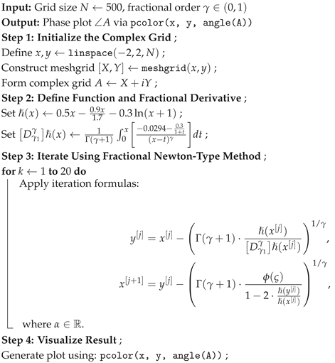
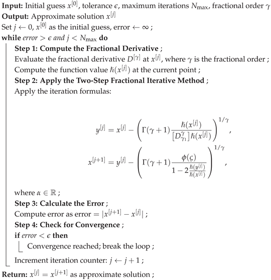
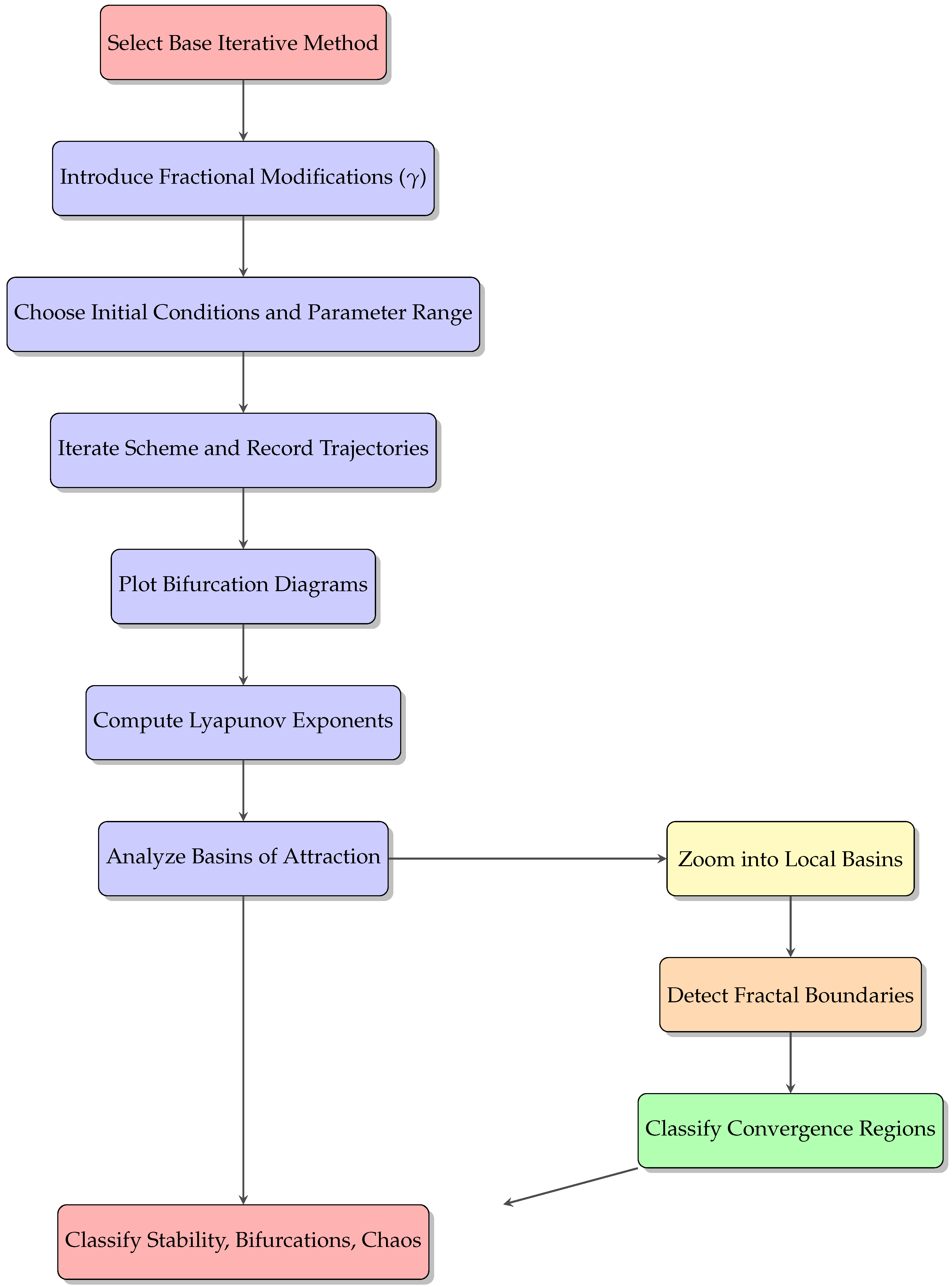
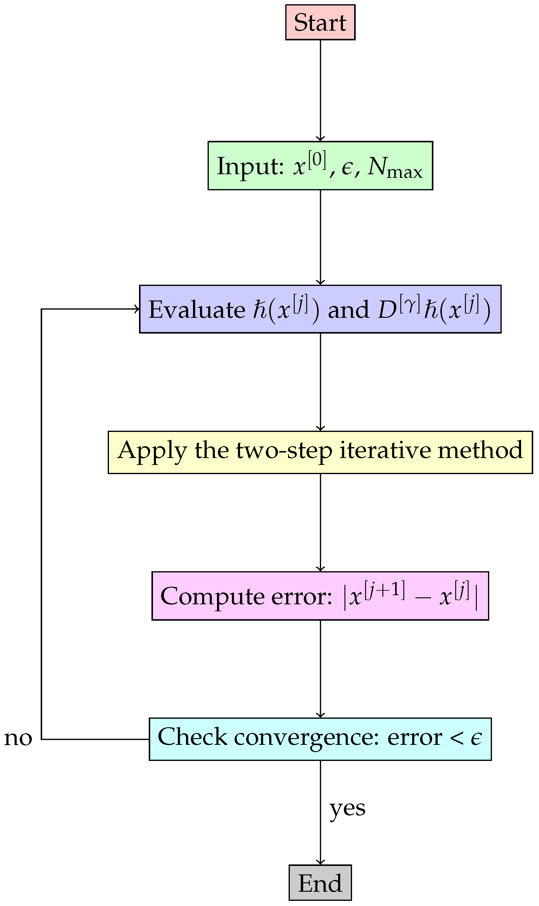
To investigate the emergence of chaos in fractional-order iterative models, we adopt a general computational framework (see the flowchart in Figure 1). This approach involves selecting a base iterative method, introducing fractional-order modifications, systematically varying key parameters, computing the resulting Lyapunov spectra and bifurcation diagrams, and analyzing the associated stability regimes. To study bifurcation and chaos in the context of fractional-order schemes, we consider the nonlinear function

$$\hslash \left(x\right)=x^3+\sigma x+1.$$

(33)

This function serves as a representative case for exploring the dynamical behavior of iterative processes, particularly under the influence of the damping parameter $\alpha$, as discussed in [24,25]. When the parameter $\alpha$  is varied within the fractional iterative method, the system exhibits significant changes in behavior. As $\alpha$  crosses certain critical values, the system transitions through different dynamical regimes—namely, stability, bifurcation, and chaos. These transitions are summarized in Table 1. 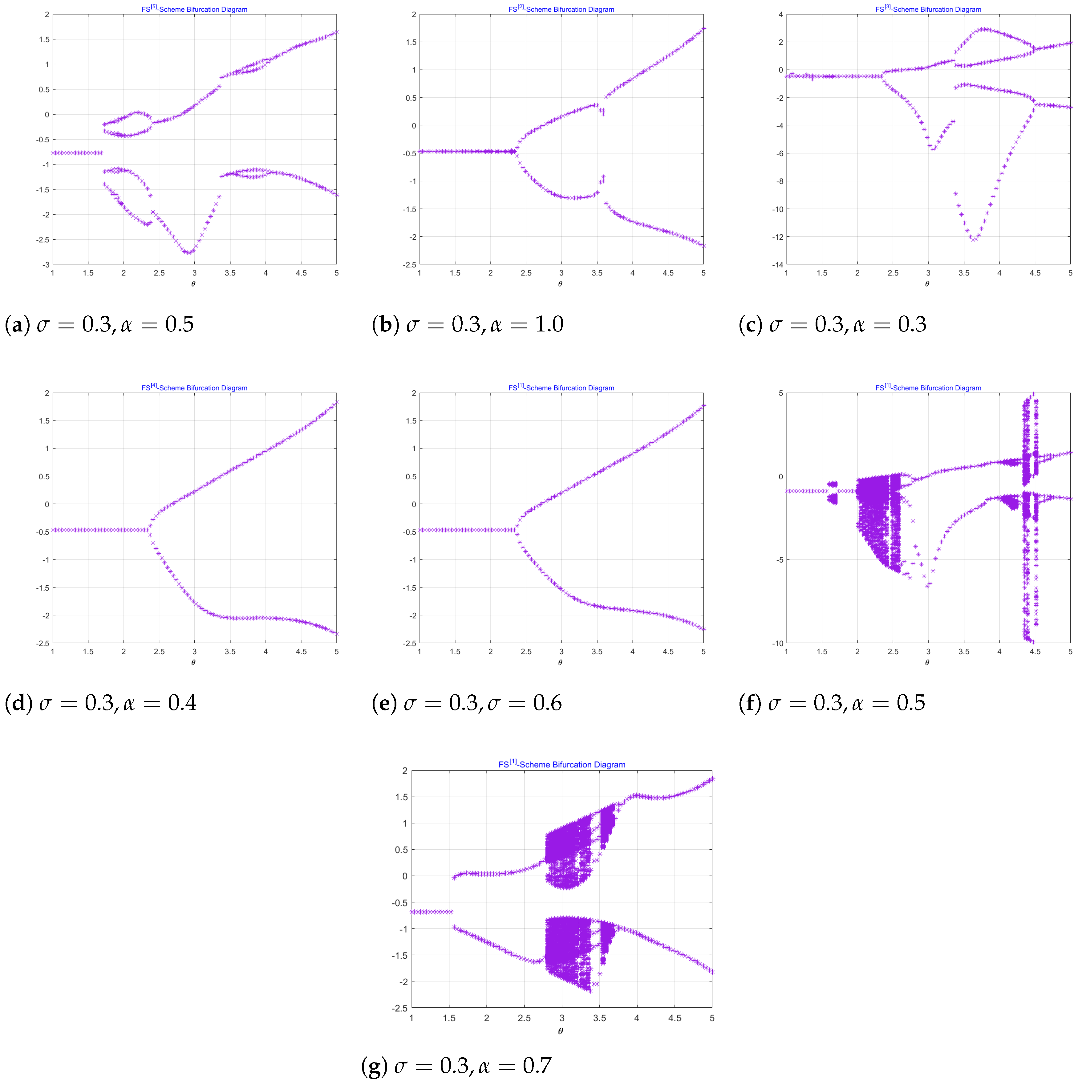Figure 2a–g present the corresponding bifurcation diagrams, where the y-axis indicates the steady-state or long-term values of the system variable and the x-axis represents values of the parameters $\sigma$  and $\alpha$. These diagrams illustrate how the nature of the solution—whether a fixed point, a periodic orbit, or a chaotic trajectory—evolves as the parameters change.

The iterative sequence remains stable for small to moderate values of $\alpha$, leading to smooth and predictable convergence toward fixed points or periodic orbits (see Figure 2a–e). As $\alpha$  increases, the system experiences period-doubling bifurcations (Figure 2c–f), transitioning from simple periodic behavior (e.g., one-period cycles) to increasingly complex periodic patterns (e.g., two-period and four-period orbits). Further increases in $\alpha$  lead to chaotic behavior in the iterative scheme (Figure 2f,g), characterized by a loss of periodicity and the emergence of irregular, scattered trajectories that exhibit high sensitivity to initial conditions.

This chaotic regime reflects the system’s strong nonlinearity and its tendency to diverge in certain parameter ranges. Deterministic chaos implies that small variations in $\alpha$  or initial values can produce significantly different outcomes. However, the system also exhibits transitional zones where, through suitable adjustments of the parameters, the dynamics can return to stability. Within these zones, the system may resume convergence to stable fixed points or periodic orbits, indicating that chaotic behavior is both parameter-dependent and potentially reversible.

Table 1 presents an analysis of the bifurcation behavior of the iterative scheme, highlighting both stable and unstable dynamical regions. The notation is as follows: $S_1^{[\ast ]}$  denotes stability; $Z_1^{[\ast ]}$  marks the onset of bifurcation; $Z_2^{[\ast ]}$  indicates period doubling; $Z_{3-4,8}^{[\ast ]}$  corresponds to higher-order periodic transitions (e.g., four-period and eight-period cycles); and $Z_C^{[\ast ]}$  represents the chaotic regime, where the scheme becomes unstable for all values of $\alpha$  and $\sigma$. All bifurcation diagrams are generated for $\gamma \approx 1$. These observations underscore the importance of carefully selecting and tuning damping parameters in iterative parallel methods, particularly in engineering applications where robustness and convergence stability are critical. The bifurcation analysis and visualizations presented in this study clearly illustrate how parameter variations influence the system’s dynamical structure and convergence behavior.

In practical applications, this approach enhances convergence stability by identifying parameter ranges that lead to chaotic dynamics and providing guidance for their adjustment. A deeper understanding of chaotic behavior in fractional iterative schemes supports the development of more reliable solvers for highly nonlinear engineering problems, including those with multiple roots, sensitive dependencies, or fractional-order characteristics.

The integration of chaos with fractional iterative schemes offers several advantages:

• Chaotic sequences enhance the exploration of the solution space, reducing the likelihood of premature convergence.
• Fractional memory effects contribute to smoother iteration behavior and mitigate abrupt changes in the solution trajectory.
• This combined strategy enables the application of iterative methods to challenging classes of nonlinear problems, such as those exhibiting multistability, sensitivity to initial conditions, or ill-posed behavior.

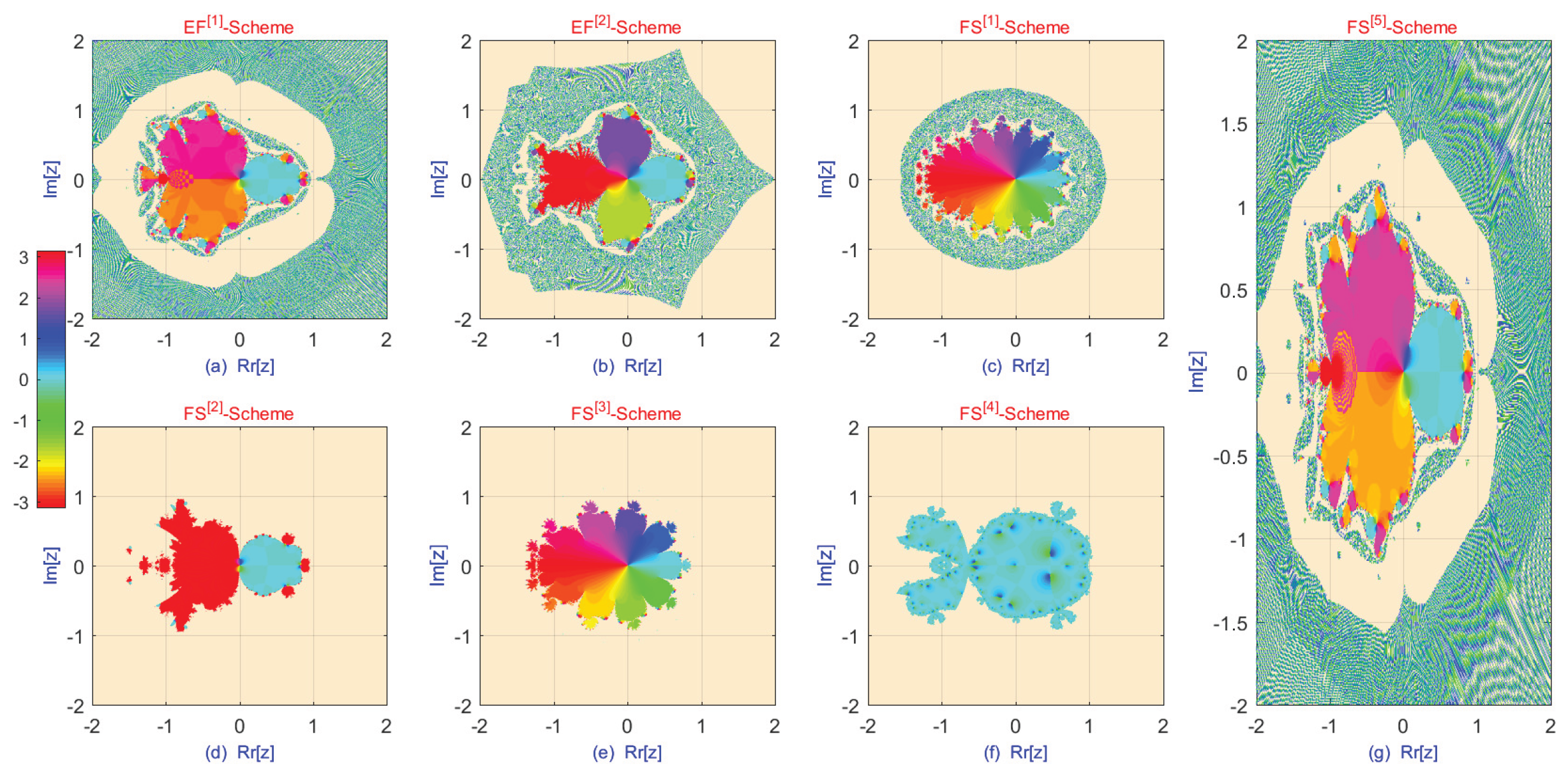
3.2. Dynamical Analysis for Parameter Tuning via Bifurcation and Chaotic Behavior

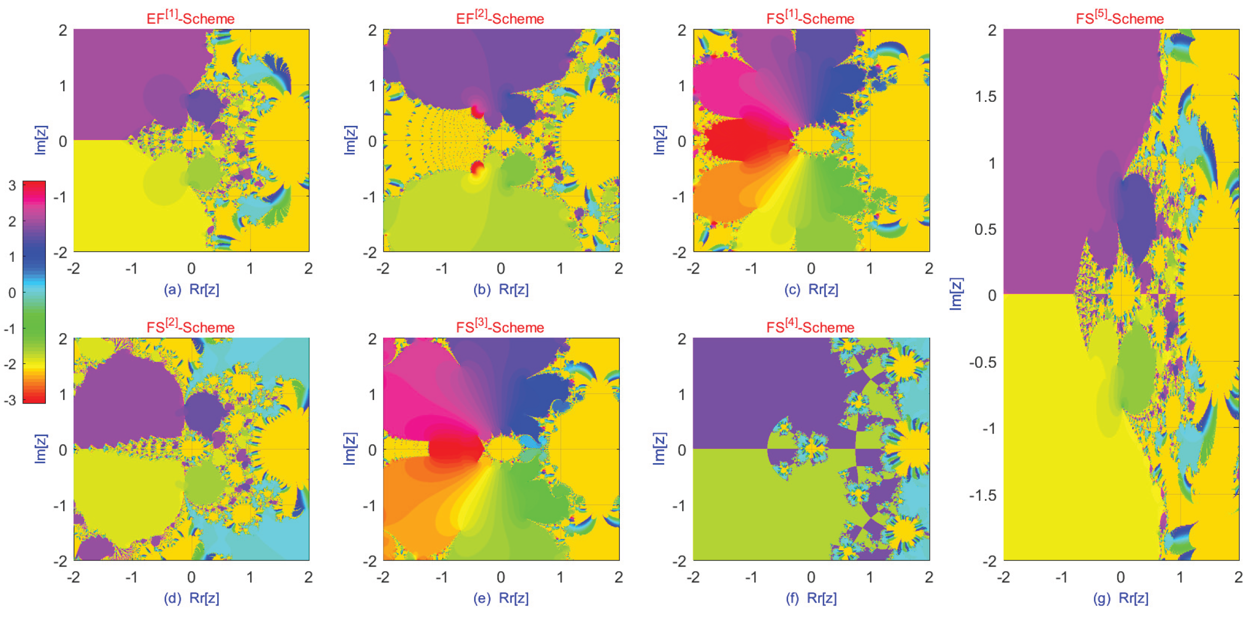
In addition to conventional analyses based on spectral radius or contraction mappings, the study of dynamical planes offers further insights into the stability properties of fractional-order iteration schemes. A dynamical plane is a graphical representation in which each point in the complex (or real) plane corresponds to an initial guess, and its color indicates the behavior of the iteration—specifically, whether it converges to a root (or attractor) or diverges [26,27,28]. In fractional-order schemes, the memory effect governed by the fractional order $\gamma$, along with any introduced chaotic perturbations, significantly influences the structure of these planes. For stable schemes, the dynamical plane typically exhibits wide, smooth, and well-separated basins of attraction associated with different roots or solutions, reflecting robustness to initial guesses. The boundaries between these basins are often fractal, indicating sensitivity to initial conditions. Lowering the fractional order $\gamma$  tends to smooth these fractal boundaries, thereby reducing sensitivity and enlarging regions of stable convergence. Properly tuned chaotic components can help prevent the iteration from becoming trapped in non-optimal attractors; however, excessive chaos may distort the basin structure, leading to fragmented or discontinuous convergence regions and signaling instability.

Moreover, dynamical planes provide a more comprehensive view of global stability than local linearization techniques. As parameters such as $\gamma$  and $\alpha$  vary, bifurcation phenomena—abrupt transitions from connected, stable basins to highly fragmented and chaotic regions—can be visually identified. This visual framework enables researchers to distinguish between stable and unstable parameter regimes and assess the robustness of an iterative method in the presence of noise or imprecise initial guesses. In engineering contexts where initial conditions are uncertain or only approximately known, this global perspective is especially valuable. Consequently, dynamical plane analysis serves as a powerful complement to traditional mathematical stability proofs, particularly for fractional-order iterative methods incorporating chaotic dynamics.

The following rational map $G\left(x\right)$  is obtained by applying the fractional order to the polynomial $p\left(x\right)=\left(x-{\vartheta }_1\right)\left(x-{\vartheta }_2\right)$, yielding

$$G\left(x\right)={\displaystyle \frac{\alpha x^8+4x^7-2\alpha x^4+24x^5+4x^3+\alpha }{2x(\alpha x^4-2\alpha x^2+8x^3+\alpha )(x^2+1)}},$$

(34)

where ${\vartheta }_1,{\vartheta }_2\in \mathbb{R}.$  By applying a Möbius transformation of the form $U\left(x\right)={\displaystyle \frac{x-a}{x-b}}$, the map $G\left(x\right)$  becomes conjugate to the function $O^{[\ast ]}\left(x\right)$, given by

$$O^{[\ast ]}\left(x\right)=UoGo{U}^{-1}\left(x\right)={\displaystyle \frac{x^3(-x^4+2\alpha x^2-2x^3+2\alpha +2x+1)}{\left(2\alpha -1\right)x^4+2\alpha x^2-2x^3+2x+1}},$$

(35)

for $\gamma \approx 1$, and this representation is independent of the parameters a and b [29]. The rational maps corresponding to other fractional-order schemes are given as follows:

$$\begin{array}{ccc}\hfill O^{[\ast ]}\left(x\right)& =& {\displaystyle \frac{x^3\left(x^8+4x^7+4x^6-4x^5+1+(4\alpha -10)x^4-4x^3+(4\alpha +4)x^3+4x\right))}{1+x^8+4x^7+(4\alpha +4)x^6-4x^5+(4\alpha -10)x^4-4x^3+4x^2+4x)}},\hfill \end{array}$$

(36)

$$\begin{array}{ccc}\hfill O^{[\ast ]}\left(x\right)& =& {\displaystyle \frac{\left(\begin{array}{c}(x^8+4.0x^7+(4.0-2.0\alpha )x^6+(-4.0-4.0\alpha )x^5+\\ (-9.6-2.0\alpha )x^4-3.2x^3+(4.0+1.2\alpha )\\ x^2+(3.2+4.0\alpha )x+0.6+2.0\alpha )x^4\end{array}\right)}{\left(\begin{array}{c}-1.+(-1.4+2.0\alpha x^8+(-4.8+4.0\alpha )x^7+(-4.+2.8\alpha )x^6+\\ 4.8x^5+(10.4-2.0\alpha )x^4+(4.0-4.0\alpha )x^3\\ +(-4.0-2.0\alpha )x^2-4.x\end{array}\right)}},\hfill \end{array}$$

(37)

$$\begin{array}{ccc}\hfill O^{[\ast ]}\left(x\right)& =& {\displaystyle \frac{x^3\left(\begin{array}{c}(x^{12}+6x^{11}+12x^{10}+2x^9-25x^8-28x^7+\\ 1+(-8\alpha +8)x^6+28x^5+7x^4-10x^3-4x^2+2x)\end{array}\right)}{\left(\begin{array}{c}-1+3x^{12}+14x^{11}+20x^{10}-6x^9-47x^8-44x^7\\ +(-8\alpha +8)x^6+44x^5+29x^4-2x^3-12x^2-6x)\end{array}\right)}},\hfill \end{array}$$

(38)

$$\begin{array}{ccc}\hfill O^{[\ast ]}\left(x\right)& =& {\displaystyle \frac{x^4\left(\begin{array}{c}{x}^{12}+6x^{11}+12x^{10}+2x^9-25x^8-28x^7+\\ 1+(-8\alpha +8)x^6+28x^5+7x^4-10x^3-4x^2+2x\end{array}\right)}{\left(\begin{array}{c}-1+3x^{12}+14x^{11}+20x^{10}-6x^9-47x^8-44x^7\\ +(-8\alpha +8)x^6+44x^5+29x^4-2x^3-12x^2-6x\end{array}\right)}},\hfill \end{array}$$

(39)

$$\begin{array}{ccc}\hfill O^{[\ast ]}\left(x\right)& =& -{\displaystyle \frac{x^3\left(\begin{array}{c}{x}^8-1+\left(6\beta -2\right)x^7+\left(16{\beta }^2-8\beta -2\right)x^6+\\ \left(24{\beta }^3-16{\beta }^2-14\beta +6\right)x^5+\\ \left(16{\beta }^4-16{\beta }^3-20{\beta }^2+26\beta \right)x^4\\ +\left(-8{\beta }^3+24{\beta }^2-4\beta -6\right)x^3+\\ \left(-4{\beta }^2-10\beta +2\right)x^2+\left(4\beta +2\right)x\end{array}\right)}{\left(\begin{array}{c}-1+x^8+\left(4\beta -2\right)x^7+\left(4{\beta }^2-10\beta -2\right)x^6+\\ \left(-8{\beta }^3-24{\beta }^2-4\beta +6\right)x^5+\\ \left(-16{\beta }^4-16{\beta }^3+20{\beta }^2+26\beta \right)x^4\\ +\left(24{\beta }^3+16{\beta }^2-14\beta -6\right)x^3+\\ \left(-16{\beta }^2-8\beta +2\right)x^2+\left(6\beta +2\right)x\end{array}\right)}},\hfill \end{array}$$

(40)

$$\begin{array}{ccc}\hfill O^{[\ast ]}\left(x\right)& =& {\displaystyle \frac{x^3(x+2)}{(2x+1}}.\hfill \end{array}$$

(41)

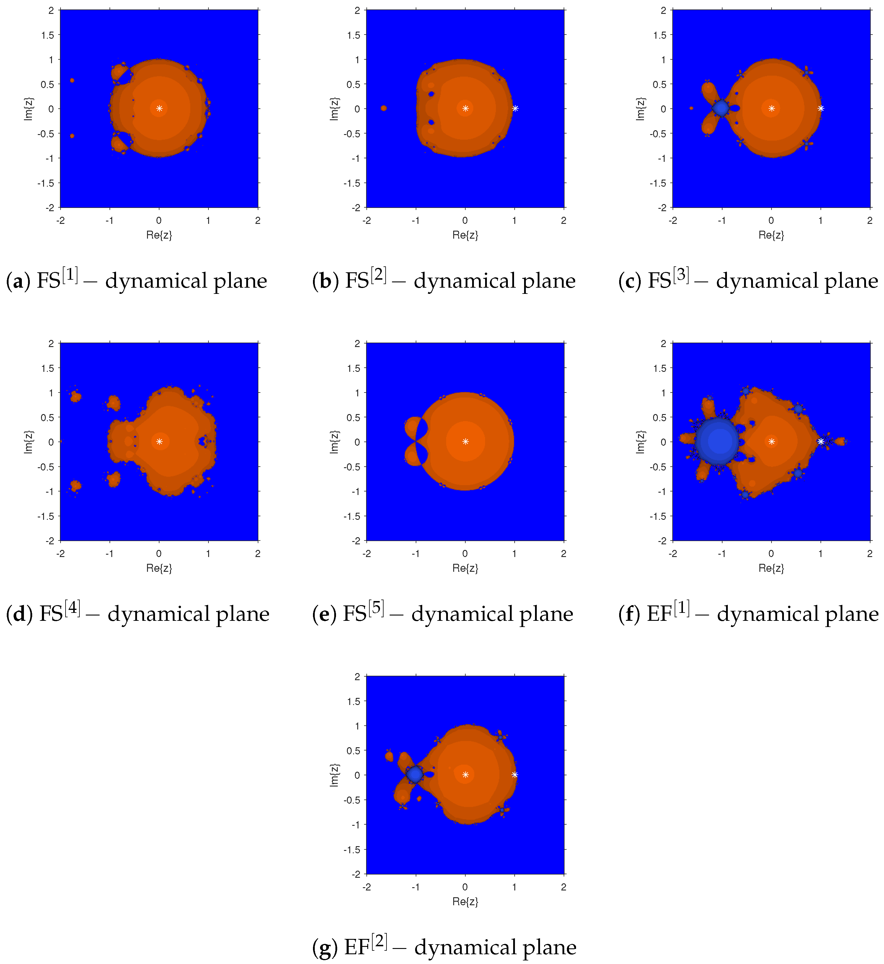
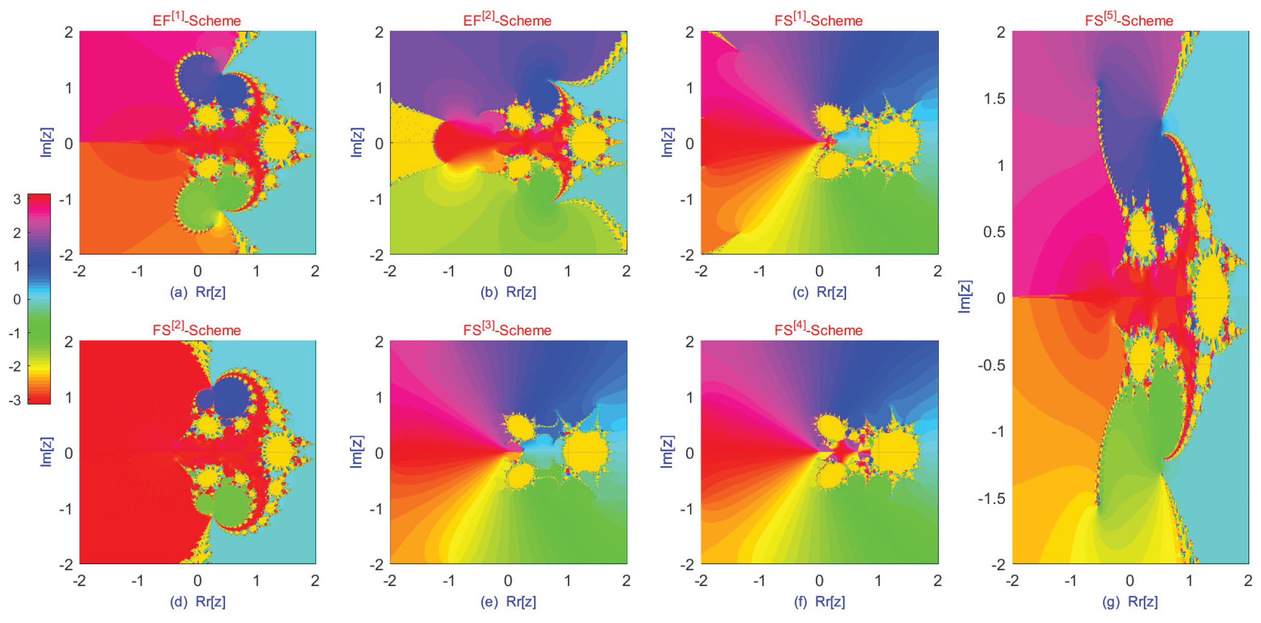
Interpretation of Dynamical Planes for Stability Analysis Using Chaos

Based on the bifurcation and chaos analysis, the values of the fractional parameter significantly affect the system’s dynamics. These changes correspond to specific regions identified in the bifurcation diagram, as outlined below:

• Smooth, Connected Basins: Selecting values of $\alpha$  and $\sigma$  from the stable region (Table 1, Column 4; Figure 2a–g), where no bifurcations are present, leads to stable dynamical behavior in the iterative schemes (Figure 3a–e).
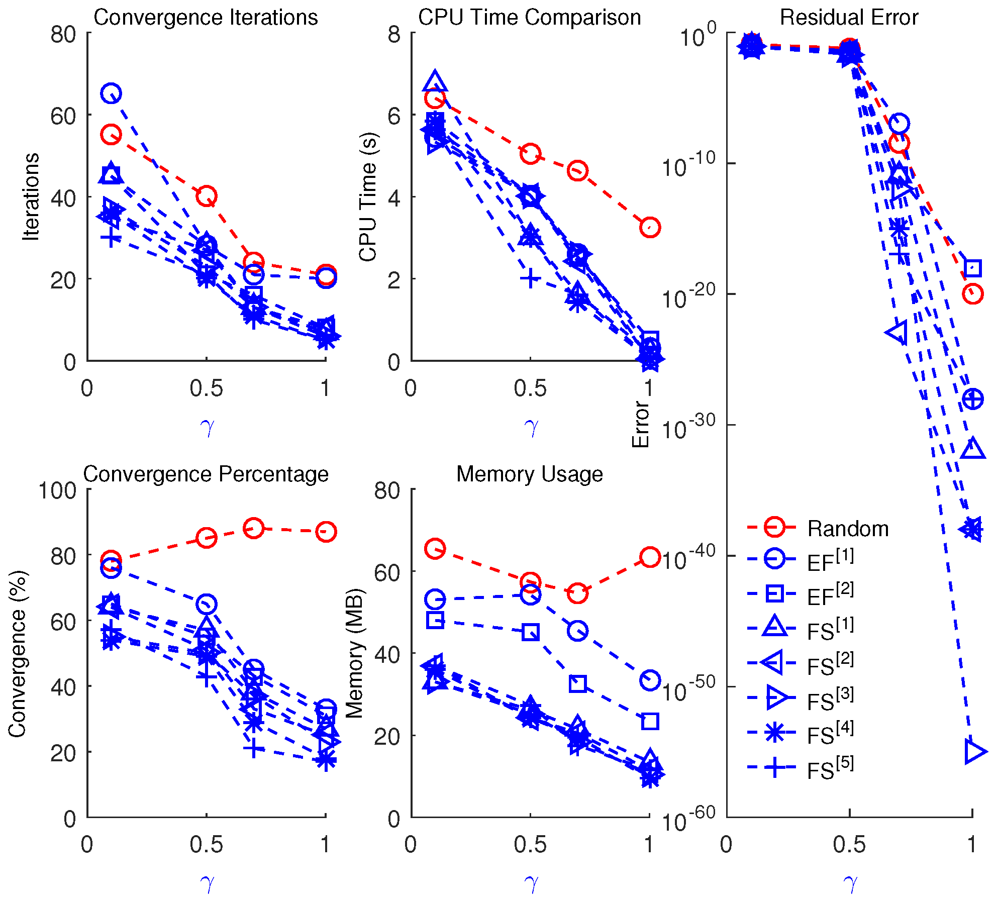
• Robust Convergence near Bifurcations: When $\alpha$  is chosen near the first or second bifurcation thresholds (Table 1, Columns 5 and 6), the dynamical plane (Figure 3f) still exhibits stability. In these cases, large basins indicate robustness, and convergence can be achieved even from coarse initial guesses, albeit at a slower rate.
• Higher-Period Bifurcation Regions: For parameter values corresponding to higher-order bifurcations (e.g., four- and eight-period cycles; see Table 1, Column 7), the schemes continue to display stable behavior, as shown in Figure 3g. However, convergence is typically slower and involves a higher computational cost.
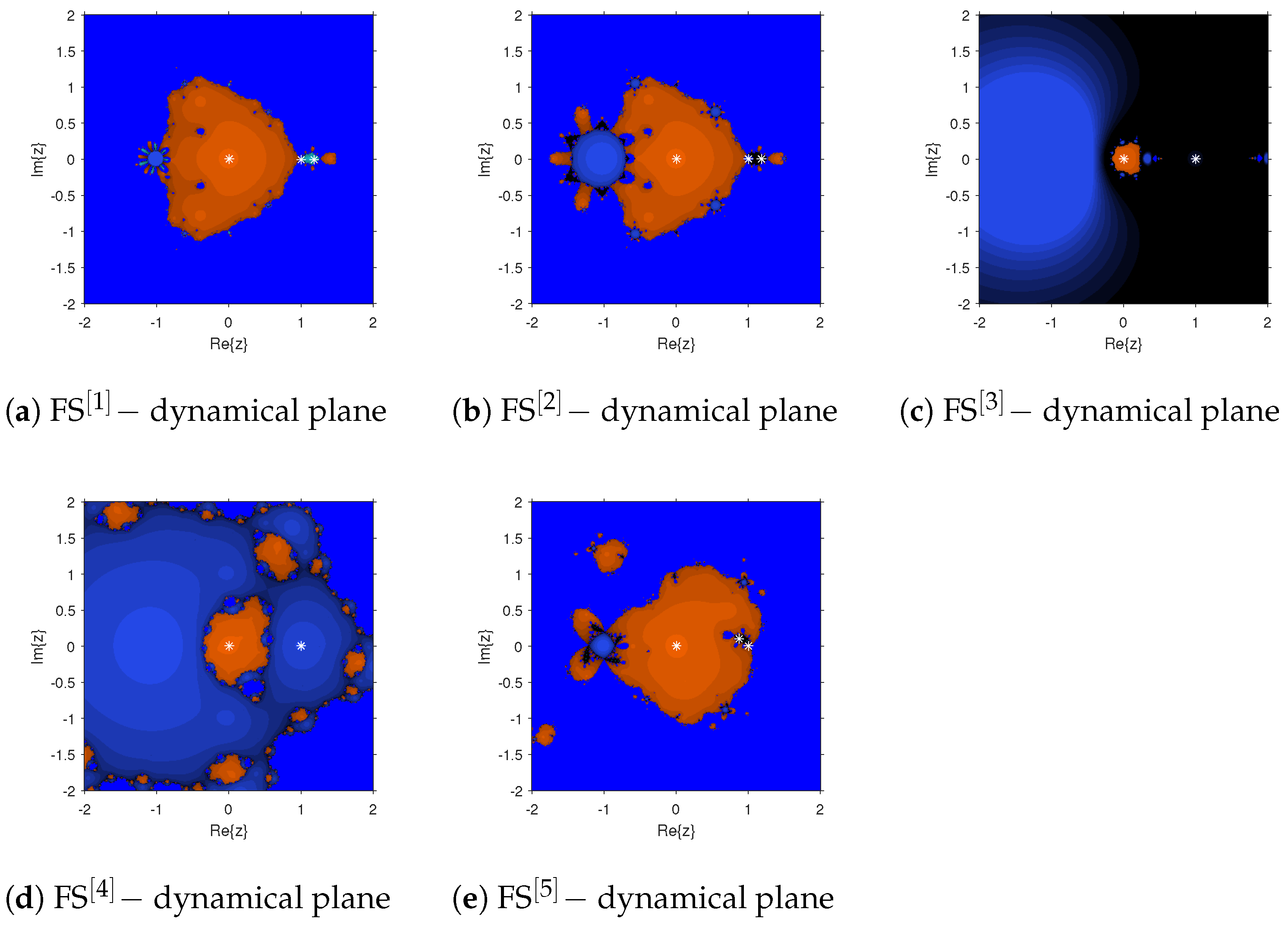
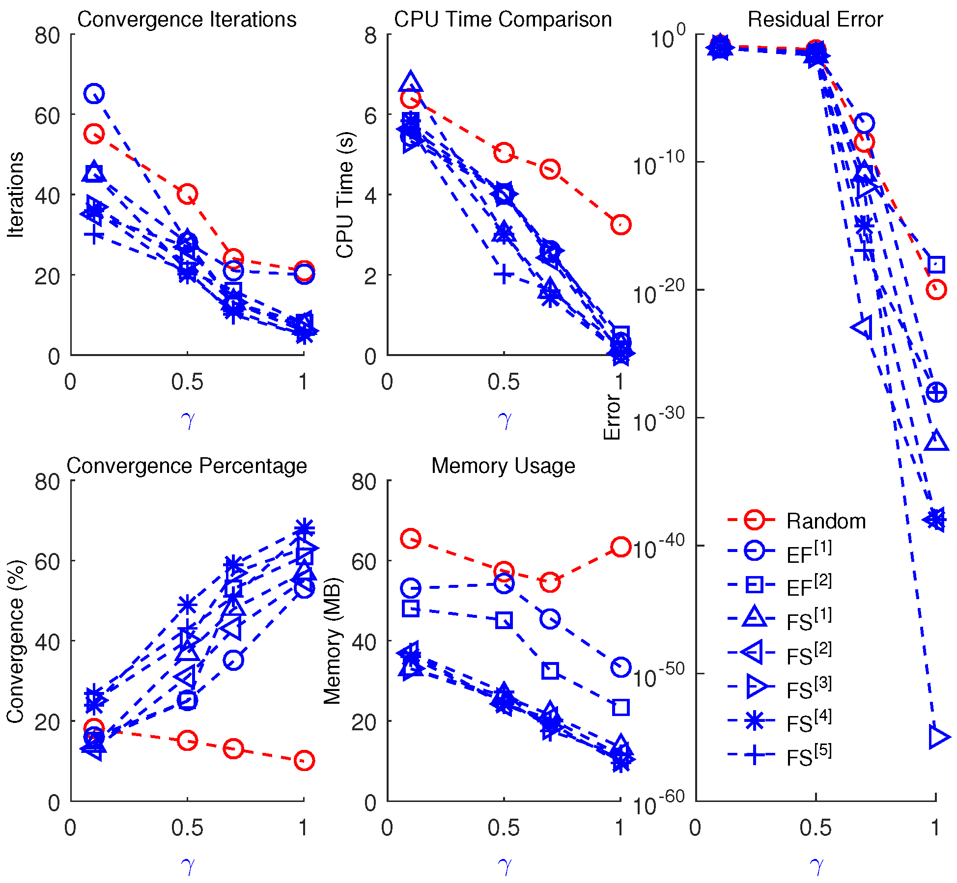
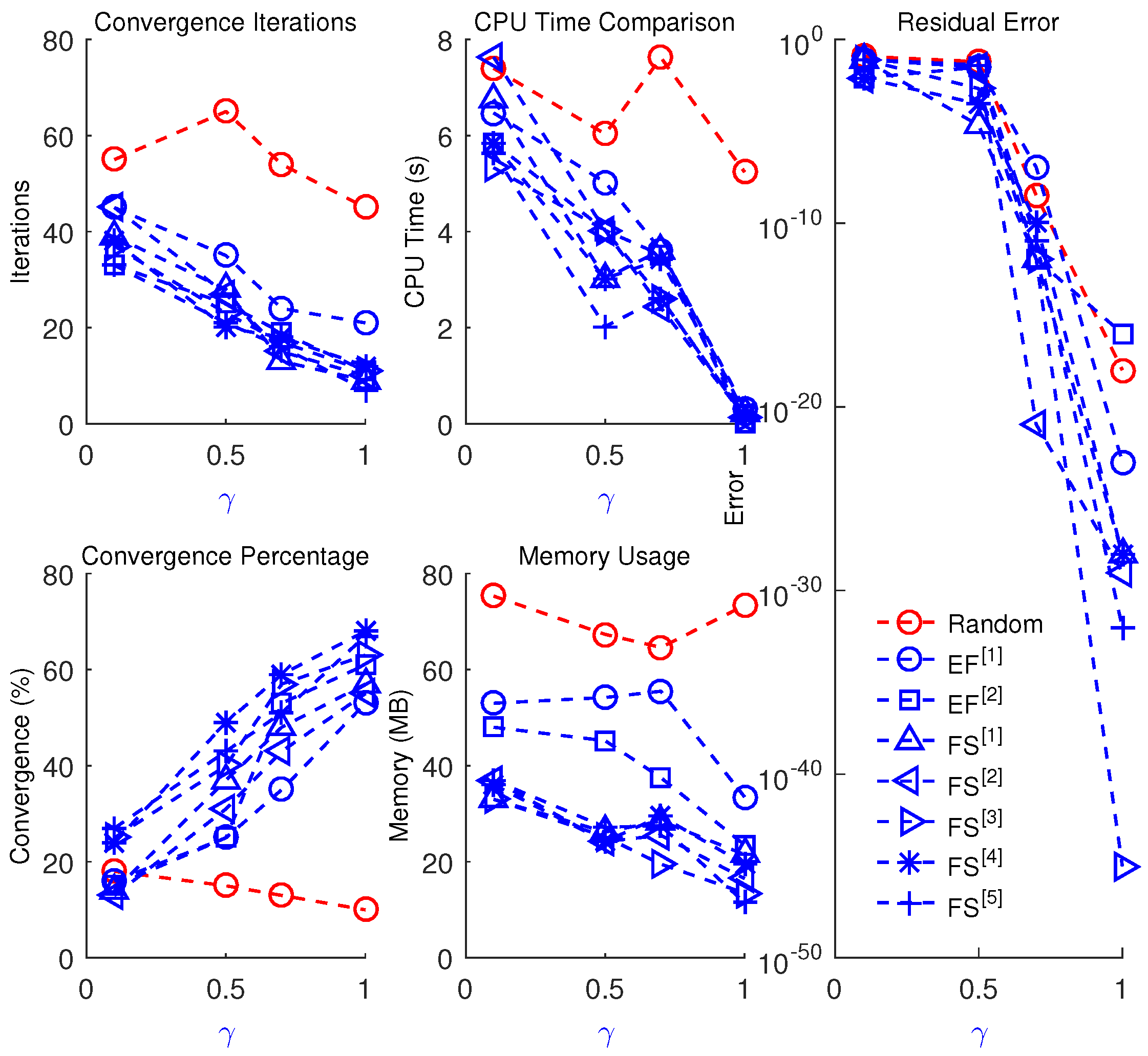
• Disconnected or Scattered Basins: In regions associated with chaotic or unstable behavior (Table 1, Column 8), the iteration may converge to unintended solutions or fail to converge altogether. These behaviors are illustrated in Figure 4a–e, where the parameter $\alpha$  lies within the chaotic regime.

4. Numerical Experiments and Performance Evaluation

The performance of the proposed two-step fractional-order iterative method is evaluated on a set of nonlinear problems arising in engineering contexts. A comparative analysis is provided, including error estimates, computational time, and benchmarks against existing iterative methods. Key evaluation criteria include the stopping condition, convergence behavior, and computational efficiency.

The proposed method is compared with conventional fractional iterative methods, such as ${\mathrm{EF}}^{\left[1\right]}$  and ${\mathrm{EF}}^{\left[2\right]}$, implemented in MATLAB 2016 using 64-digit floating-point arithmetic. The primary metrics used for assessing algorithmic performance are outlined below:

(1)

Stopping Criterion: The algorithm terminates when the absolute difference between successive iterates satisfies the following condition:

$$ϵ=\left|x^{\left[j+1\right]}-x^{\left[j\right]}\right|<tol,$$

(42)

where $ϵ$  is the error tolerance, typically set to ${10}^{-18}$.

(2)

CPU Time: The total computational time required for convergence is used as a measure of efficiency. Time is recorded using MATLAB’s tic and toc functions.

(3)

Error Analysis: The following error metrics are considered:

–

Percentage Error: The relative error between two consecutive approximations is given by

$$\mathrm{Percentage}\mathrm{Error}={\displaystyle \frac{\left|x^{\left[j+1\right]}-x^{\left[j\right]}\right|}{\left|x^{\left[j\right]}\right|}}\times 100.$$

(43)

–

Convergence Rate: The ratio of errors between successive iterations is used to assess the rate at which convergence occurs. This is computed using Algorithms 1 and 2 and illustrated in the flowchart in Figure 5.

(4)

Comparison with Existing Methods: The proposed method is evaluated against existing classical techniques, such as the ${\mathrm{EF}}^{\left[1\right]}$  and ${\mathrm{EF}}^{\left[2\right]}$  methods. The comparison focuses on the following:

–

Convergence Speed: How quickly the method approaches the solution.

–

Accuracy: The degree to which the computed solution approximates the exact one.

–

Computational Efficiency: The computational resources required to achieve convergence.

Algorithm 1: Fractal generation via fractional scheme

Algorithm 2: Two-step fractional-order scheme for solving nonlinear problems

4.1. Enzyme Kinetics with Inhibition (Biochemical Reactions)  [30]

Enzyme kinetics with inhibition is a key framework in biochemical reaction modeling. It describes how enzymes bind to substrates to catalyze reactions and how this process is influenced by the presence of inhibitors. The classical Michaelis–Menten equation can be extended to incorporate inhibitory effects, resulting in nonlinear formulations. Inhibition may occur through competitive, non-competitive, or uncompetitive mechanisms, each of which alters the enzyme–substrate interaction differently. A representative nonlinear formulation that incorporates inhibition effects is given by

$$\hslash \left(x\right)=k_{1}x-{\displaystyle \frac{k_{2}x}{K_m}}-k_{3}ln\left(x+1\right),$$

(44)

where x denotes the substrate concentration, and $k_1$, $k_2$, and $k_3$  are rate constants characterizing the reaction. The logarithmic term accounts for more complex regulatory effects, such as enzyme cooperativity or allosteric modulation. This mathematical formulation plays a central role in modeling processes like drug metabolism, metabolic control, and signal transduction, where inhibitors and activators are critically involved. The nonlinear nature of the system underscores the importance of employing advanced computational methods for the accurate prediction and analysis of biochemical dynamics.

For steady-state analysis, the system can be approximated by the following nonlinear function using the fixed parameter values $k_1=0.5$, $k_2=0.9$, $k_3=0.3$, and $K_m=1.7$:

$$\hslash \left(x\right)=0.5x-{\displaystyle \frac{0.9x}{1.7}}-0.3ln\left(x+1\right).$$

(45)

The corresponding Caputo fractional derivative of order $\gamma$  is given by

$$\left[D_{{\gamma }_1}^{\gamma }\right]\hslash \left(x\right)={\displaystyle \frac{1}{\mathrm{\Gamma }\left(\gamma +1\right)}}\underset{0}{\overset{x}{\int }}\left[{\displaystyle \frac{-0.0294-\frac{0.3}{1+t}}{{(x-t)}^{\gamma }}}\right]dt.$$

(46)

The exact root of this nonlinear model is $0.0$, and the initial guess used for the iterative scheme is $x^{\left[0\right]}=0.3$. The numerical results for the fractional-order schemes, both with and without chaos-based parameter tuning, are presented in

Table 2. Performance of fractional schemes without chaos-optimized parameter tuning for solving Equation (45).

Metric	Iterations	C-Time	M-Usage	P-Con	M-Err
${\mathrm{EF}}^{\left[1\right]}$	22	$5.432$	$67.424$	$19.342$	$2.52\times {10}^{-9}$
${\mathrm{EF}}^{\left[2\right]}$	21	$4.024$	$74.325$	$11.765$	$0.53\times {10}^{-7}$
${\mathrm{FS}}^{\left[1\right]}$	23	$3.142$	$65.932$	$17.439$	$6.63\times {10}^{-11}$
${\mathrm{FS}}^{\left[2\right]}$	16	$3.524$	$55.327$	$25.325$	$0.43\times {10}^{-21}$
${\mathrm{FS}}^{\left[3\right]}$	17	$4.442$	$31.403$	$45.897$	$1.76\times {10}^{-39}$
${\mathrm{FS}}^{\left[4\right]}$	18	$3.204$	$49.540$	$28.942$	$5.47\times {10}^{-25}$
${\mathrm{FS}}^{\left[5\right]}$	15	$3.642$	$41.542$	$22.342$	$5.63\times {10}^{-19}$

,

Table 3. Dynamical performance analysis of fractional schemes ${\mathrm{FS}}^{\left[1\right]}$ –${\mathrm{FS}}^{\left[5\right]}$  and ${\mathrm{EF}}^{\left[1\right]}$ –${\mathrm{EF}}^{\left[2\right]}$  for solving Equation (45).

Metric	${\mathrm{EF}}^{\left[1\right]}$	${\mathrm{EF}}^{\left[2\right]}$	${\mathrm{FS}}^{\left[1\right]}$	${\mathrm{FS}}^{\left[2\right]}$	${\mathrm{FS}}^{\left[3\right]}$	${\mathrm{FS}}^{\left[4\right]}$	${\mathrm{FS}}^{\left[5\right]}$
E−time	$2.1348$	$2.3453$	$2.543$	$3.755$	$2.0054$	$4.7655$	$1.63254$
M-usage	$75.432$	$78.543$	$45.765$	$43.654$	$33.546$	$23.654$	$20.887$
P-convergence	$65.45$	$67.56$	$68.67$	$87.56$	$34.45$	$35.43$	$26.453$

and

Table 4. Error and consistency analysis of fractional-order schemes ${\mathrm{EF}}^{\left[1\right]}$ –${\mathrm{EF}}^{\left[2\right]}$  and ${\mathrm{FS}}^{\left[1\right]}$ –${\mathrm{FS}}^{\left[5\right]}$  for solving Equation (45) across different values of fractional parameter $\gamma$.

Metric	M-Err	C-Time	M-Err	C-Time	M-Err	C-Time	M-Err	C-Time
$\gamma$	$0.3$		$0.5$		$0.7$		$0.9$
${\mathrm{EF}}^{\left[1\right]}$	$8.9\times {10}^{-3}$	$5.4$	$8.5\times {10}^{-5}$	$2.8$	$8.5\times {10}^{-15}$	$1.5$	$8.5\times {10}^{-65}$	$1.01$
${\mathrm{EF}}^{\left[2\right]}$	$6.8\times {10}^{-2}$	$4.0$	$6.8\times {10}^{-7}$	$3.4$	$8.5\times {10}^{-15}$	$1.4$	$6.8\times {10}^{-47}$	$1.7$
${\mathrm{FS}}^{\left[1\right]}$	$1.7\times {10}^{-6}$	$3.1$	$0.6\times {10}^{-6}$	$2.3$	$0.6\times {10}^{-46}$	$0.0$	$0.6\times {10}^{-86}$	$0.4$
${\mathrm{FS}}^{\left[2\right]}$	$3.0\times {10}^{-5}$	$3.5$	$0.4\times {10}^{-5}$	$3.0$	$0.4\times {10}^{-45}$	$0.5$	$0.4\times {10}^{-85}$	$0.5$
${\mathrm{FS}}^{\left[3\right]}$	$3.1\times {10}^{-9}$	$4.4$	$9.1\times {10}^{-9}$	$4.6$	$1.1\times {10}^{-59}$	$0.4$	$1.9\times {10}^{-79}$	$0.01$
${\mathrm{FS}}^{\left[4\right]}$	$1.7\times {10}^{-1}$	$3.0$	$5.7\times {10}^{-2}$	$3.7$	$5.7\times {10}^{-65}$	$0.4$	$6.4\times {10}^{-86}$	$0.02$
${\mathrm{FS}}^{\left[5\right]}$	$0.5\times {10}^{-7}$	$3.6$	$0.6\times {10}^{-7}$	$2.6$	$5.9\times {10}^{-59}$	$0.3$	$1.4\times {10}^{-89}$	$0.01$

for solving Equation (45).

Table 4 and

Table 5. Memory usage, percentage convergence, and stability analysis of fractional-order schemes ${\mathrm{EF}}^{\left[1\right]}$ –${\mathrm{EF}}^{\left[2\right]}$  and ${\mathrm{FS}}^{\left[1\right]}$ –${\mathrm{FS}}^{\left[5\right]}$  for solving Equation (45) across different values of fractional parameter $\gamma$.

Metric	M-Usage	P-Con	M-Usage	P-Con	M-Usage	P-Con	M-Usage	P-Con
$\gamma$	$0.3$		$0.5$		$0.7$		$0.9$
${\mathrm{EF}}^{\left[1\right]}$	$88.65$	$12.8$	$79.65$	$22.73$	$68.34$	$22.33$	$55.05$	$32.7$
${\mathrm{EF}}^{\left[2\right]}$	$89.34$	$9.6$	$81.34$	$26.23$	$76.34$	$27.22$	$53.07$	$49.2$
${\mathrm{FS}}^{\left[1\right]}$	$65.60$	$14.2$	$45.60$	$24.03$	$55.65$	$25.03$	$35.54$	$76.3$
${\mathrm{FS}}^{\left[2\right]}$	$55.65$	$11.6$	$32.08$	$29.73$	$31.53$	$37.73$	$24.09$	$73.7$
${\mathrm{FS}}^{\left[3\right]}$	$46.23$	$14.2$	$21.10$	$34.23$	$43.07$	$45.2$	$37.54$	$75.2$
${\mathrm{FS}}^{\left[4\right]}$	$47.87$	$13.6$	$26.04$	$43.00$	$19.08$	$65.12$	$35.43$	$62.2$
${\mathrm{FS}}^{\left[5\right]}$	$41.65$	$15.2$	$31.65$	$31.2\%$	$34.67$	$51.05$	$31.65$	$70.4$

illustrate the cross-validation results obtained during training and testing, highlighting the proposed method’s stability, consistency, memory efficiency, and accuracy.

The dynamical behavior of the proposed scheme, in comparison with existing methods, is presented in Table 3 and Figure 6. As shown in Table 3, the proposed approaches demonstrate improved performance, characterized by reduced generation time of the basins of attraction (E-time) and a higher percentage of convergence.

In Table 4, C-time refers to the computational time in seconds, M-Err denotes the absolute residual error (as defined in (42)), and P-con represents the percentage convergence (as defined in (43)). Table 4 presents the error and consistency analysis, while Table 5 reports the memory utilization, percentage convergence, and stability evaluation of the fractional schemes applied to the biomedical engineering model described in Section 4.1. The numerical results indicate that the proposed methods offer improvements over existing approaches in terms of residual error, memory efficiency, convergence rate, and the number of iterations required to meet the desired accuracy for given fractional and optimized parameter values. Furthermore, Table 4 and Table 5 show that increasing the value of $\gamma$  from 0.1 to 1.0 leads to enhanced convergence, stability, and consistency compared with the ${\mathrm{EF}}^{\left[1\right]}$  and ${\mathrm{EF}}^{\left[2\right]}$  methods.

Table 6. Numerical outcomes of fractional schemes ${\mathrm{FS}}^{\left[1\right]}$ –${\mathrm{FS}}^{\left[5\right]}$  and ${\mathrm{EF}}^{\left[1\right]}$ –${\mathrm{EF}}^{\left[2\right]}$  compared with randomly selected parameters for solving Equation (45) with different values of fractional parameter $\gamma$.

Metric	Iterations	C-Time	M-Usage	P-Con	Error
		$\gamma =0.5$
Random	55	7.023	78.77	$9.54\%$	$1.6\times {10}^{-2}$
${\mathrm{EF}}^{\left[1\right]}$	40	5.030	57.56	$12.73\%$	$8.5\times {10}^{-2}$
${\mathrm{EF}}^{\left[2\right]}$	28	4.025	54.43	$33.23\%$	$8.5\times {10}^{-1}$
${\mathrm{FS}}^{\left[1\right]}$	21	4.543	45.54	$31.03\%$	$0.6\times {10}^{-4}$
${\mathrm{FS}}^{\left[2\right]}$	28	3.543	26.65	$27.73\%$	$0.4\times {10}^{-3}$
${\mathrm{FS}}^{\left[3\right]}$	27	4.546	24.65	$25.23\%$	$1.1\times {10}^{-4}$
${\mathrm{FS}}^{\left[4\right]}$	23	3.436	23.76	$23.73\%$	$5.7\times {10}^{-3}$
${\mathrm{FS}}^{\left[5\right]}$	20	2.543	21.78	$21.03\%$	$5.9\times {10}^{-3}$
		$\gamma =0.7$
Random	55	7.435	77.54	$8.73\%$	$0.5\times {10}^{-2}$
${\mathrm{EF}}^{\left[1\right]}$	24	4.632	54.56	$13.73\%$	$2.1\times {10}^{-2}$
${\mathrm{EF}}^{\left[2\right]}$	21	2.003	45.43	$43.23\%$	$1.5\times {10}^{-11}$
${\mathrm{FS}}^{\left[1\right]}$	16	2.783	32.54	$30.03\%$	$2.4\times {10}^{-10}$
${\mathrm{FS}}^{\left[2\right]}$	13	1.598	21.65	$37.73\%$	$3.4\times {10}^{-9}$
${\mathrm{FS}}^{\left[3\right]}$	12	2.509	29.65	$35.23\%$	$3.4\times {10}^{-14}$
${\mathrm{FS}}^{\left[4\right]}$	11	2.443	18.76	$53.73\%$	$5.7\times {10}^{-9}$
${\mathrm{FS}}^{\left[5\right]}$	10	1.543	14.78	$41.03\%$	$0.3\times {10}^{-11}$
		$\gamma =0.9$
Random	68	7.124	87.87	$7.98\%$	$1.1\times {10}^{-2}$
${\mathrm{EF}}^{\left[1\right]}$	21	5.030	63.36	$15.73\%$	$8.5\times {10}^{-19}$
${\mathrm{EF}}^{\left[2\right]}$	20	1.025	33.43	$45.23\%$	$8.5\times {10}^{-29}$
${\mathrm{FS}}^{\left[1\right]}$	8	2.543	25.54	$43.03\%$	$0.3\times {10}^{-19}$
${\mathrm{FS}}^{\left[2\right]}$	7	0.043	20.65	$58.73\%$	$2.4\times {10}^{-33}$
${\mathrm{FS}}^{\left[3\right]}$	8	0.046	11.65	$81.23\%$	$3.4\times {10}^{-39}$
${\mathrm{FS}}^{\left[4\right]}$	6	0.036	10.76	$62.73\%$	$7.9\times {10}^{-56}$
${\mathrm{FS}}^{\left[5\right]}$	5	0.003	18.78	$63.03\%$	$7.6\times {10}^{-39}$

and Figure 7 present the overall performance of the proposed scheme. When $\gamma \approx 1$, and under random perturbations, the following observations can be made in comparison with existing methods:

• The number of iterations required by the proposed scheme decreases significantly.
• Higher relative accuracy is obtained, with a lower residual error for the fractional scheme.
• Percentage convergence improves, while CPU time and memory usage are reduced.

4.2. Extended Glucose–Insulin Regulatory Model  [31]

The glucose–insulin homeostasis model is fundamental for understanding the mechanisms that regulate blood glucose levels, particularly in the context of diabetes. It describes the dynamic relationship between glucose levels in the blood and insulin secretion by the pancreas. This regulation is governed by complex feedback loops in which insulin lowers glucose levels, while glucose concentration in turn influences insulin production. The model is typically expressed through nonlinear equations involving polynomials and logarithmic terms, where the glucose concentration is modeled as a function of insulin levels and time. These nonlinearities account for physiological effects such as saturation and thresholds in the feedback system:

$$\hslash \left(x\right)={\left(x-G_0\right)}^3-alog\left(x+1\right),$$

(47)

where x represents the glucose concentration and $G_0$  is the basal glucose level. This formulation plays a critical role in simulating and controlling glucose dynamics in diabetic patients and supports the development of therapeutic strategies. By fixing $G_0=0.5$  and $a=0.3$, the model becomes

$$\hslash \left(x\right)={\left(x-0.5\right)}^3-0.3log\left(x+1\right).$$

(48)

The Caputo-order fractional derivative of this function is given by

$$\left[D_{{\gamma }_1}^{\gamma }\right]\hslash \left(x\right)=\left[D_{{\gamma }_1}^{\gamma }\right]\hslash \left(x\right)={\displaystyle \frac{1}{\mathrm{\Gamma }\left(\gamma +1\right)}}\underset{0}{\overset{x}{\int }}\left[{\displaystyle \frac{3\left(t-0.5\right)-\frac{0.3}{t+1}}{{(x-t)}^{\gamma }}}\right]dt.$$

(49)

The exact root of the nonlinear model is $-0.9999869889$, and the corresponding initial guess is $x^{\left[0\right]}=-1.7i$.

Table 7. Numerical outcomes of fractional schemes without chaos-optimized parameter values for solving Equation (48).

Metric	Iterations	C-Time	M-Usage	P-Con	M-Err
${\mathrm{EF}}^{\left[1\right]}$	19	$6.456$	$71.434$	$18.332$	$1.13\times {10}^{-7}$
${\mathrm{EF}}^{\left[2\right]}$	20	$6.113$	$84.332$	$15.545$	$5.03\times {10}^{-5}$
${\mathrm{FS}}^{\left[1\right]}$	25	$5.354$	$71.002$	$16.764$	$3.54\times {10}^{-9}$
${\mathrm{FS}}^{\left[2\right]}$	18	$4.355$	$65.332$	$21.655$	$9.99\times {10}^{-23}$
${\mathrm{FS}}^{\left[3\right]}$	20	$5.346$	$51.883$	$32.117$	$7.06\times {10}^{-27}$
${\mathrm{FS}}^{\left[4\right]}$	19	$4.887$	$59.764$	$25.002$	$6.08\times {10}^{-20}$
${\mathrm{FS}}^{\left[5\right]}$	17	$4.654$	$51.653$	$21.653$	$0.76\times {10}^{-23}$

,

Table 8. Dynamical performance analysis of fractional schemes ${\mathrm{FS}}^{\left[1\right]}$ –${\mathrm{FS}}^{\left[5\right]}$  and ${\mathrm{EF}}^{\left[1\right]}$ –${\mathrm{EF}}^{\left[2\right]}$  for solving Equation (48).

Metric	${\mathrm{EF}}^{\left[1\right]}$	${\mathrm{EF}}^{\left[2\right]}$	${\mathrm{FS}}^{\left[1\right]}$	${\mathrm{FS}}^{\left[2\right]}$	${\mathrm{FS}}^{3]}$	${\mathrm{FS}}^{\left[4\right]}$	${\mathrm{FS}}^{\left[5\right]}$
E−time	$6.5404$	$5.5465$	$2.4375$	$2.0055$	$1.9874$	$1.7655$	$0.8874$
M-usage	$86.432$	$76.435$	$55.353$	$43.654$	$33.546$	$32.009$	$24.887$
P-convergence	$75.645$	$57.2873$	$86.867$	$87.0769$	$84.055$	$75.069$	$86.86$

and

Table 9. Error and consistency analysis of fractional schemes for solving Equation (48) with varying values of $\gamma$.

Metric	M-Err	C-Time	M-Err	C-Time	M-Err	C-Time	M-Err	C-Time
$\gamma$	$0.3$		$0.5$		$0.7$		$0.9$
${\mathrm{EF}}^{\left[1\right]}$	$1.1\times {10}^{-3}$	$7.1$	$8.5\times {10}^{-3}$	$3.6$	$8.5\times {10}^{-16}$	$1.5$	$8.5\times {10}^{-85}$	$1.8$
${\mathrm{EF}}^{\left[2\right]}$	$0.8\times {10}^{-3}$	$6.4$	$6.8\times {10}^{-4}$	$4.9$	$6.8\times {10}^{-13}$	$1.7$	$6.8\times {10}^{-47}$	$1.6$
${\mathrm{FS}}^{\left[1\right]}$	$0.9\times {10}^{-2}$	$6.6$	$0.6\times {10}^{-9}$	$4.6$	$0.6\times {10}^{-41}$	$0.1$	$0.6\times {10}^{-96}$	$0.4$
${\mathrm{FS}}^{\left[2\right]}$	$6.7\times {10}^{-5}$	$4.6$	$0.4\times {10}^{-11}$	$3.7$	$0.4\times {10}^{-31}$	$0.7$	$0.4\times {10}^{-115}$	$0.3$
${\mathrm{FS}}^{\left[3\right]}$	$3.5\times {10}^{-4}$	$4.9$	$7.1\times {10}^{-14}$	$4.6$	$3.3\times {10}^{-39}$	$0.8$	$0.9\times {10}^{-169}$	$0.3$
${\mathrm{FS}}^{\left[4\right]}$	$3.4\times {10}^{-6}$	$5.7$	$0.4\times {10}^{-11}$	$3.7$	$6.4\times {10}^{-31}$	$0.7$	$6.6\times {10}^{-115}$	$0.2$
${\mathrm{FS}}^{\left[5\right]}$	$1.2\times {10}^{-5}$	$4.9$	$2.8\times {10}^{-15}$	$4.6$	$5.5\times {10}^{-43}$	$0.8$	$1.7\times {10}^{-141}$	$0.1$

present the numerical results obtained using fractional schemes, both with and without chaos-optimized parameters, for solving Equation (48).

Table 9 and

Table 10. Memory usage, percentage convergence, and stability analysis of fractional schemes for solving Equation (48) with varying values of $\gamma$.

Metric	M-Usage	P-Con	M-Usage	P-Con	M-Usage	P-Con	M-Usage	P-Con
$\gamma$	$0.3$		$0.5$		$0.7$		$0.9$
${\mathrm{EF}}^{\left[1\right]}$	$75.12$	$8.8$	$65.34$	$12.7$	$56.34$	$45.7$	$31.87$	$80.7$
${\mathrm{EF}}^{\left[2\right]}$	$87.54$	$9.1$	$67.98$	$19.2$	$47.35$	$54.8$	$29.43$	$86.2$
${\mathrm{FS}}^{\left[1\right]}$	$56.12$	$10.0$	$55.34$	$13.2$	$35.76$	$67.3$	$22.98$	$93.2$
${\mathrm{FS}}^{\left[2\right]}$	$63.23$	$16.7$	$53.34$	$26.7$	$33.23$	$76.3$	$21.88$	$97.3$
${\mathrm{FS}}^{\left[3\right]}$	$59.76$	$16.9$	$49.34$	$26.6$	$38.74$	$65.6$	$23.54$	$99.7$
${\mathrm{FS}}^{\left[4\right]}$	$54.09$	$15.8$	$43.23$	$25.3$	$38.98$	$70.1$	$19.32$	$92.2$
${\mathrm{FS}}^{\left[5\right]}$	$58.23$	$17.8$	$39.23$	$30.2$	$31.67$	$62.0$	$20.12$	$90.4$

present cross-validation results from both training and testing phases, illustrating the improved stability, consistency, memory efficiency, and accuracy of the proposed method.

The dynamical behavior of the proposed scheme, in comparison with existing approaches, is presented in Table 8 and Figure 8. As shown in Table 8, the proposed methods exhibit improved performance in terms of reduced generation time (E−time) for the basin of attraction and higher percentage convergence.

Table 9 presents the error and consistency analysis, while Table 10 summarizes memory utilization, percentage convergence, and stability performance for the fractional schemes applied to the biomedical engineering model described in Section 4.2. The numerical results indicate that the proposed methods achieve lower error, improved memory efficiency, and higher convergence percentages and require fewer iterations to reach the desired accuracy, particularly when using chaos-optimized and fractional parameter values. Furthermore, the data in Table 9 and Table 10 show that increasing the value of $\gamma$  from 0.1 to 1.0 leads to notable improvements in convergence rate, stability, and consistency compared with the ${\mathrm{EF}}^{\left[1\right]}$  and ${\mathrm{EF}}^{\left[2\right]}$  methods.

Table 11. Overall performance of fractional-order schemes ${\mathrm{FS}}^{\left[1\right]}$ –${\mathrm{FS}}^{\left[5\right]}$  and ${\mathrm{EF}}^{\left[1\right]}$ –${\mathrm{EF}}^{\left[2\right]}$, and a random perturbation strategy for solving Equation (48) for varying values of $\gamma$. Results are compared in terms of iterations, CPU time, memory usage, percentage convergence, and error.

Metric	Iterations	C-Time	M-Usage	P-Con	Error
		$\gamma =0.5$
Random	67	6.030	87.56	$09.73\%$	$8.5\times {10}^{-2}$
${\mathrm{EF}}^{\left[1\right]}$	57	5.324	65.34	$13.63\%$	$7.5\times {10}^{-2}$
${\mathrm{EF}}^{\left[2\right]}$	50	5.025	64.43	$10.43\%$	$0.5\times {10}^{-1}$
${\mathrm{FS}}^{\left[1\right]}$	55	5.543	55.54	$13.43\%$	$0.6\times {10}^{-2}$
${\mathrm{FS}}^{\left[2\right]}$	51	4.543	36.65	$15.23\%$	$0.4\times {10}^{-3}$
${\mathrm{FS}}^{\left[3\right]}$	45	5.546	54.65	$17.34\%$	$0.1\times {10}^{-2}$
${\mathrm{FS}}^{\left[4\right]}$	48	5.436	53.76	$18.74\%$	$8.0\times {10}^{-2}$
${\mathrm{FS}}^{\left[5\right]}$	47	4.543	61.78	$15.03\%$	$0.3\times {10}^{-1}$
		$\gamma =0.7$
Random	68	7.764	87.23	$9.22\%$	$7.9\times {10}^{-4}$
${\mathrm{EF}}^{\left[1\right]}$	65	6.632	54.56	$13.73\%$	$2.1\times {10}^{-3}$
${\mathrm{EF}}^{\left[2\right]}$	33	5654	45.13	$43.23\%$	$1.5\times {10}^{-4}$
${\mathrm{FS}}^{\left[1\right]}$	37	3.234	52.04	$30.03\%$	$2.4\times {10}^{-5}$
${\mathrm{FS}}^{\left[2\right]}$	33	4.124	43.08	$37.73\%$	$3.4\times {10}^{-5}$
${\mathrm{FS}}^{\left[3\right]}$	31	3.653	57.11	$35.23\%$	$3.4\times {10}^{-6}$
${\mathrm{FS}}^{\left[4\right]}$	33	3.554	58.23	$53.73\%$	$5.7\times {10}^{-5}$
${\mathrm{FS}}^{\left[5\right]}$	29	3.543	54.65	$41.03\%$	$0.3\times {10}^{-5}$
		$\gamma =0.9$
Random	55	5.054	87.36	$15.87\%$	$8.5\times {10}^{-19}$
${\mathrm{EF}}^{\left[1\right]}$	17	3.054	63.36	$15.23\%$	$8.5\times {10}^{-19}$
${\mathrm{EF}}^{\left[2\right]}$	18	3.655	33.43	$45.09\%$	$8.5\times {10}^{-29}$
${\mathrm{FS}}^{\left[1\right]}$	11	2.987	25.54	$43.43\%$	$0.3\times {10}^{-19}$
${\mathrm{FS}}^{\left[2\right]}$	12	2.435	20.65	$48.76\%$	$2.4\times {10}^{-33}$
${\mathrm{FS}}^{\left[3\right]}$	10	0.231	11.65	$51.65\%$	$3.4\times {10}^{-39}$
${\mathrm{FS}}^{\left[4\right]}$	11	0.132	10.76	$52.23\%$	$7.9\times {10}^{-46}$
${\mathrm{FS}}^{\left[5\right]}$	13	0.321	18.78	$53.43\%$	$7.6\times {10}^{-39}$

and Figure 9 present the overall performance evaluation. The results indicate that when $\gamma \approx 1$, the proposed method demonstrates improved behavior under random perturbations compared with existing approaches. Specifically,

• The number of iterations required by the proposed scheme decreases significantly.
• Higher relative accuracy is achieved, as evidenced by a lower residual error of the fractional scheme.
• The method attains a higher percentage of convergence while requiring less CPU time and memory.

4.3. Drug Dose–Response Model [32]

A drug dose–response model describes how a biological system responds to varying concentrations of a drug. Key parameters in this model include the maximum effect ($E_{max}$), the half-maximal effective concentration ($C_a^n$), and the exponent (n), which reflects the steepness of the dose–response curve. The model captures how the pharmacological effect increases with dosage until a saturation point is reached. Solving the corresponding nonlinear equation allows for the determination of the drug concentration required to achieve a target biological response. The dose–response relationship can be modeled using the following nonlinear equation:

$$R\left(x\right)={\displaystyle \frac{E_{max}{x}^n}{C_a^n+x^n}},$$

(50)

where $R\left(x\right)$  is the observed response, and the objective is to determine the drug concentration x that produces this response. Rearranging the equation yields the following nonlinear form:

$$f\left(x\right)={\displaystyle \frac{E_{max}{x}^n}{C_a^n+x^n}}-R.$$

(51)

We consider the following parameter values:

• $E_{max}=100$  (maximum effect, e.g., % inhibition).
• $C_a^n=5$  (drug concentration in $\mathrm{\mu }\mathrm{M}$).
• $n=2$  (steepness factor).
• $R=60$  (observed response).

By substituting them into (51), we obtain the nonlinear equation

$$f\left(x\right)={\displaystyle \frac{100x^2}{25+x^2}}-60=0.$$

(52)

The Caputo-order fractional derivative of the function is given by

$$\left[D_{{\gamma }_1}^{\gamma }\right]\hslash \left(x\right)=\left[D_{{\gamma }_1}^{\gamma }\right]\hslash \left(x\right)={\displaystyle \frac{1}{\mathrm{\Gamma }\left(\gamma +1\right)}}\underset{0}{\overset{x}{\int }}\left[\left({\displaystyle \frac{200x}{25+x^2}}-{\displaystyle \frac{{\left(200x\right)}^3}{{\left(25+x^2\right)}^2}}\right){\displaystyle \frac{1}{{(x-t)}^{\gamma }}}\right]dt.$$

(53)

The exact root of this nonlinear model is $\zeta =6.123724357$, and the corresponding initial guess is $x^{\left[0\right]}=5.1$.

Table 12. Numerical performance of fractional-order schemes ${\mathrm{FS}}^{\left[1\right]}$ –${\mathrm{FS}}^{\left[5\right]}$  and ${\mathrm{EF}}^{\left[1\right]}$ –${\mathrm{EF}}^{\left[2\right]}$  without chaos-optimized parameters for solving Equation (52).

Metric	Iterations	C-Time	M-Usage	P-Con	M-Err
${\mathrm{EF}}^{\left[1\right]}$	31	$7.875$	$94.874$	$7.342$	$2.011\times {10}^{-2}$
${\mathrm{EF}}^{\left[2\right]}$	30	$8.453$	$91.115$	$6.765$	$0.573\times {10}^{-3}$
${\mathrm{FS}}^{\left[1\right]}$	25	$5.986$	$71.002$	$13.439$	$0.653\times {10}^{-9}$
${\mathrm{FS}}^{\left[2\right]}$	23	$5.321$	$65.765$	$19.325$	$6.473\times {10}^{-10}$
${\mathrm{FS}}^{\left[3\right]}$	19	$6.042$	$61.325$	$23.897$	$7.786\times {10}^{-11}$
${\mathrm{FS}}^{\left[4\right]}$	21	$5.144$	$69.607$	$21.942$	$0.423\times {10}^{-15}$
${\mathrm{FS}}^{\left[5\right]}$	19	$4.872$	$51.776$	$18.342$	$8.645\times {10}^{-15}$

,

Table 13. Dynamical analysis of fractional-order schemes ${\mathrm{FS}}^{\left[1\right]}$ –${\mathrm{FS}}^{\left[5\right]}$  and ${\mathrm{EF}}^{\left[1\right]}$ –${\mathrm{EF}}^{\left[2\right]}$  for solving Equation (52). Metrics include execution time, memory usage, and percentage convergence.

Metric	${\mathrm{EF}}^{\left[1\right]}$	${\mathrm{EF}}^{\left[2\right]}$	${\mathrm{FS}}^{\left[1\right]}$	${\mathrm{FS}}^{\left[2\right]}$	${\mathrm{FS}}^{3]}$	${\mathrm{FS}}^{\left[4\right]}$	${\mathrm{FS}}^{\left[5\right]}$
E−time	$7.6545$	$8.6546$	$2.0098$	$1.4045$	$2.9004$	$0.2015$	$0.0014$
M-usage	$87.545$	$89.085$	$65.983$	$45.345$	$33.765$	$32.545$	$19.435$
P-convergence	$25.65$	$29.23$	$89.07$	$90.07$	$93.05$	$94.09$	$97.43$

,

Table 14. Error and consistency analysis of fractional schemes for solving Equation (52).

Metric	M-Err	C-Time	M-Err	C-Time	M-Err	C-Time	M-Err	C-Time
$\gamma$	$0.3$		$0.5$		$0.7$		$0.9$
${\mathrm{EF}}^{\left[1\right]}$	$1.1\times {10}^{-3}$	$7.1$	$8.5\times {10}^{-3}$	$3.6$	$8.5\times {10}^{-6}$	$1.5$	$8.5\times {10}^{-8}$	$2.8$
${\mathrm{EF}}^{\left[2\right]}$	$0.8\times {10}^{-3}$	$6.4$	$6.8\times {10}^{-4}$	$4.9$	$6.8\times {10}^{-7}$	$1.7$	$6.8\times {10}^{-9}$	$2.6$
${\mathrm{FS}}^{\left[1\right]}$	$0.9\times {10}^{-2}$	$6.6$	$0.6\times {10}^{-9}$	$4.6$	$0.6\times {10}^{-41}$	$0.1$	$0.6\times {10}^{-96}$	$0.4$
${\mathrm{FS}}^{\left[2\right]}$	$6.7\times {10}^{-5}$	$4.6$	$0.4\times {10}^{-11}$	$3.7$	$0.4\times {10}^{-31}$	$0.7$	$0.4\times {10}^{-115}$	$0.3$
${\mathrm{FS}}^{\left[3\right]}$	$3.5\times {10}^{-4}$	$4.9$	$7.1\times {10}^{-14}$	$4.6$	$3.3\times {10}^{-39}$	$0.8$	$0.9\times {10}^{-169}$	$0.3$
${\mathrm{FS}}^{\left[4\right]}$	$3.4\times {10}^{-6}$	$5.7$	$0.4\times {10}^{-11}$	$3.7$	$6.4\times {10}^{-31}$	$0.7$	$6.6\times {10}^{-115}$	$0.2$
${\mathrm{FS}}^{\left[5\right]}$	$1.2\times {10}^{-5}$	$4.9$	$2.8\times {10}^{-15}$	$4.6$	$5.5\times {10}^{-43}$	$0.8$	$1.7\times {10}^{-141}$	$0.1$

and

Table 15. Memory usage, percentage convergence, and stability analysis of fractional technique for solving (52).

Metric	M-Usage	P-Con	M-Usage	P-Con	M-Usage	P-Con	M-Usage	P-Con
$\gamma$	$0.3$		$0.5$		$0.7$		$0.9$
${\mathrm{EF}}^{\left[1\right]}$	$75.12$	$8.8$	$65.34$	$12.7$	$56.34$	$45.7$	$31.87$	$48.7$
${\mathrm{EF}}^{\left[2\right]}$	$87.54$	$9.1$	$67.98$	$19.2$	$47.35$	$54.8$	$29.43$	$56.2$
${\mathrm{FS}}^{\left[1\right]}$	$56.12$	$10.0$	$55.34$	$13.2$	$35.76$	$67.3$	$22.98$	$93.2$
${\mathrm{FS}}^{\left[2\right]}$	$63.23$	$16.7$	$53.34$	$26.7$	$33.23$	$76.3$	$21.88$	$97.3$
${\mathrm{FS}}^{\left[3\right]}$	$59.76$	$16.9$	$49.34$	$26.6$	$38.74$	$65.6$	$23.54$	$99.7$
${\mathrm{FS}}^{\left[4\right]}$	$54.09$	$15.8$	$43.23$	$25.3$	$38.98$	$70.1$	$19.32$	$92.2$
${\mathrm{FS}}^{\left[5\right]}$	$58.23$	$17.8$	$39.23$	$30.2$	$31.67$	$62.0$	$20.12$	$90.4$

present the numerical results obtained using fractional schemes with and without the chaos-optimized parameter for solving Equation (52).

Table 13, Table 14 and Table 15 present cross-validation results for both training and testing phases, demonstrating the improved stability, consistency, memory efficiency, and accuracy of the proposed method compared with existing approaches.

The dynamical behavior of the proposed scheme, compared with existing methods, is summarized in Table 13 and illustrated in Figure 10. As shown in Table 13, the proposed approach exhibits improved performance, characterized by reduced generation time for the basin of attraction (E-time) and a higher percentage of convergence.

Table 14 presents the error and consistency analysis, while Table 15 reports the memory usage, percentage convergence, and stability assessment of the fractional schemes applied to the biomedical engineering model described in Section 4.3. The numerical results indicate that the proposed methods yield improved performance over existing techniques, particularly in terms of error reduction, memory efficiency, convergence rate, and the number of iterations required to reach the desired accuracy under chaos-optimized and fractional parameter settings. Moreover, Table 14 and Table 15 show that increasing the fractional order $\gamma$  from 0.1 to 1.0 enhances the convergence speed, stability, and consistency relative to the ${\mathrm{EF}}^{\left[1\right]}$ –${\mathrm{EF}}^{\left[2\right]}$  methods.

Table 16. Overall performance analysis of fractional schemes in chaos-based, dynamic, and random perturbation settings across varying values of $\gamma$  for solving (52).

Metric	Iterations	C-Time	M-Usage	P-Con	Error
		$\gamma =0.5$
Random	67	7.876	87.56	$7.73\%$	$8.5\times {10}^{-2}$
${\mathrm{EF}}^{\left[1\right]}$	57	6.324	77.34	$9.63\%$	$7.5\times {10}^{-1}$
${\mathrm{EF}}^{\left[2\right]}$	50	6.087	75.23	$9.43\%$	$0.5\times {10}^{-1}$
${\mathrm{FS}}^{\left[1\right]}$	55	5.543	55.54	$13.43\%$	$0.6\times {10}^{-2}$
${\mathrm{FS}}^{\left[2\right]}$	51	4.543	36.65	$15.23\%$	$0.4\times {10}^{-3}$
${\mathrm{FS}}^{\left[3\right]}$	45	5.546	54.65	$17.34\%$	$0.1\times {10}^{-2}$
${\mathrm{FS}}^{\left[4\right]}$	48	5.436	53.76	$18.74\%$	$8.0\times {10}^{-2}$
${\mathrm{FS}}^{\left[5\right]}$	47	4.543	61.78	$15.03\%$	$0.3\times {10}^{-1}$
		$\gamma =0.7$
Random	65	7.632	78.87	$7.73\%$	$5.7\times {10}^{-3}$
${\mathrm{EF}}^{\left[1\right]}$	45	6.632	54.43	$9.73\%$	$9.0\times {10}^{-3}$
${\mathrm{EF}}^{\left[2\right]}$	46	5654	45.13	$8.55\%$	$0.5\times {10}^{-3}$
${\mathrm{FS}}^{\left[1\right]}$	37	3.234	52.04	$30.03\%$	$2.4\times {10}^{-5}$
${\mathrm{FS}}^{\left[2\right]}$	33	4.124	43.08	$37.73\%$	$3.4\times {10}^{-5}$
${\mathrm{FS}}^{\left[3\right]}$	31	3.653	57.11	$35.23\%$	$3.4\times {10}^{-6}$
${\mathrm{FS}}^{\left[4\right]}$	33	3.554	58.23	$53.73\%$	$5.7\times {10}^{-5}$
${\mathrm{FS}}^{\left[5\right]}$	29	3.543	54.65	$41.03\%$	$0.3\times {10}^{-5}$
		$\gamma =0.9$
Random	55	7.054	87.36	$9.54\%$	$1.0\times {10}^{-3}$
${\mathrm{EF}}^{\left[1\right]}$	33	4.054	73.36	$12.03\%$	$2.1\times {10}^{-5}$
${\mathrm{EF}}^{\left[2\right]}$	37	6.655	67.43	$11.32\%$	$8.5\times {10}^{-7}$
${\mathrm{FS}}^{\left[1\right]}$	11	2.987	25.54	$43.43\%$	$0.3\times {10}^{-19}$
${\mathrm{FS}}^{\left[2\right]}$	12	2.435	20.65	$48.76\%$	$2.4\times {10}^{-33}$
${\mathrm{FS}}^{\left[3\right]}$	10	0.231	11.65	$51.65\%$	$3.4\times {10}^{-39}$
${\mathrm{FS}}^{\left[4\right]}$	11	0.132	10.76	$52.23\%$	$7.9\times {10}^{-46}$
${\mathrm{FS}}^{\left[5\right]}$	13	0.321	18.78	$53.43\%$	$7.6\times {10}^{-39}$

and Figure 11 summarize the overall performance of the proposed scheme under random perturbations and for $\gamma \approx 1$, in comparison with existing methods. The results indicate that

• The number of iterations required for convergence is significantly reduced.
• Higher relative accuracy is achieved, as reflected by a lower residual error in the fractional scheme.
• A greater percentage of successful convergences is observed, along with reduced CPU and memory usage.

4.4. Lung Volume and Pressure (Static Compliance Curve) [33]

The lung volume–pressure relationship, commonly described by the static compliance curve, is fundamental in characterizing the mechanical properties of the lungs, particularly their capacity to expand in response to applied pressure. This relationship is governed by the elastic properties of lung tissue and airway resistance and is typically expressed using a nonlinear function such as the arctangent model:

$$f\left(x\right)=Aarctan\left(B\left(x-C\right)\right)-D,$$

(54)

where x denotes the applied pressure, and $A,B,C,D\in \mathbb{R}$. The curve generally displays saturation behavior at higher pressures, where additional increases in pressure result in minimal changes in lung volume. This nonlinearity is essential to accurately modeling both healthy and pathological lung conditions, including chronic obstructive pulmonary disease (COPD) and pulmonary fibrosis. It also plays a crucial role in the design and optimization of mechanical ventilation systems.

For steady-state analysis, the model can be approximated by the following nonlinear function by setting the parameters $A=0.1$, $B=0.3$, $C=0.8$, and $D=0.9$:

$$\hslash \left(x\right)=0.1arctan\left(0.3\left(x-0.8\right)\right)-0.9.$$

(55)

The Caputo-order fractional derivative of this function is expressed as

$$\left[D_{{\gamma }_1}^{\gamma }\right]\hslash \left(x\right)=\left[D_{{\gamma }_1}^{\gamma }\right]\hslash \left(x\right)={\displaystyle \frac{1}{\mathrm{\Gamma }\left(\gamma +1\right)}}\underset{0}{\overset{x}{\int }}\left[{\displaystyle \frac{0.03}{1+0.09{\left(t-0.8\right)}^2}}{\displaystyle \frac{1}{{(x-t)}^{\gamma }}}\right]dt.$$

(56)

The exact root of this nonlinear model is $\xi =0.7077$, with an initial starting value of $x^{\left[0\right]}=-1.3$.

Table 17. Numerical outcomes of fractional schemes without using the chaos-optimized parameter for solving (55).

Metric	Iterations	C-Time	M-Usage	P-Con	M-Err
${\mathrm{EF}}^{\left[1\right]}$	18	$4.932$	$41.657$	$27.029$	$2.52\times {10}^{-19}$
${\mathrm{EF}}^{\left[2\right]}$	17	$4.605$	$44.543$	$21.798$	$2.44\times {10}^{-16}$
${\mathrm{FS}}^{\left[1\right]}$	15	$4.187$	$35.345$	$37.769$	$0.03\times {10}^{-21}$
${\mathrm{FS}}^{\left[2\right]}$	13	$3.653$	$29.124$	$35.115$	$9.48\times {10}^{-31}$
${\mathrm{FS}}^{\left[3\right]}$	11	$3.882$	$27.675$	$45.007$	$5.78\times {10}^{-39}$
${\mathrm{FS}}^{\left[4\right]}$	7	$3.325$	$35.214$	$48.998$	$8.87\times {10}^{-35}$
${\mathrm{FS}}^{\left[5\right]}$	7	$2.001$	$31.764$	$58.768$	$0.61\times {10}^{-49}$

,

Table 18. Dynamical analysis of selected fractional schemes ${\mathrm{EF}}^{\left[1\right]}$ –${\mathrm{EF}}^{\left[2\right]}$, ${\mathrm{FS}}^{\left[1\right]}$ –${\mathrm{FS}}^{\left[2\right]}$, ${\mathrm{EF}}^{\left[3\right]}$, and ${\mathrm{EF}}^{\left[4\right]}$ –${\mathrm{EF}}^{\left[5\right]}$  for solving (55).

Metric	${\mathrm{EF}}^{\left[1\right]}$	${\mathrm{EF}}^{\left[2\right]}$	${\mathrm{FS}}^{\left[1\right]}$	${\mathrm{FS}}^{\left[2\right]}$	${\mathrm{FS}}^{3]}$	${\mathrm{FS}}^{\left[4\right]}$	${\mathrm{FS}}^{\left[5\right]}$
E−time	$6.1348$	$5.3453$	$3.647$	$1.7505$	$1.0084$	$0.7655$	$0.0354$
M-usage	$78.432$	$73.098$	$59.325$	$51.876$	$46.324$	$34.436$	$17.924$
P-convergence	$65.45$	$67.56$	$68.67$	$87.56$	$34.45$	$35.43$	$26.453$

,

Table 19. Error and consistency analysis of various fractional-order schemes for solving (55) for different values of $\gamma$.

Metric	M-Err	C-Time	M-Err	C-Time	M-Err	C-Time	M-Err	C-Time
$\gamma$	$0.3$		$0.5$		$0.7$		$0.9$
${\mathrm{EF}}^{\left[1\right]}$	$3.2\times {10}^{-4}$	$5.6$	$8.5\times {10}^{-5}$	$2.1$	$8.5\times {10}^{-15}$	$1.5$	$8.5\times {10}^{-65}$	$1.8$
${\mathrm{EF}}^{\left[2\right]}$	$0.1\times {10}^{-5}$	$6.8$	$6.8\times {10}^{-7}$	$3.8$	$6.8\times {10}^{-17}$	$1.4$	$6.8\times {10}^{-47}$	$1.5$
${\mathrm{FS}}^{\left[1\right]}$	$5.7\times {10}^{-6}$	$5.3$	$0.6\times {10}^{-16}$	$2.3$	$0.6\times {10}^{-46}$	$0.3$	$0.6\times {10}^{-86}$	$0.3$
${\mathrm{FS}}^{\left[2\right]}$	$8.7\times {10}^{-5}$	$5.1$	$0.4\times {10}^{-15}$	$3.7$	$0.4\times {10}^{-45}$	$0.3$	$0.4\times {10}^{-85}$	$0.2$
${\mathrm{FS}}^{\left[3\right]}$	$8.5\times {10}^{-6}$	$4.3$	$1.4\times {10}^{-16}$	$4.4$	$1.4\times {10}^{-59}$	$0.4$	$1.4\times {10}^{-139}$	$0.1$
${\mathrm{FS}}^{\left[4\right]}$	$5.4\times {10}^{-7}$	$3.7$	$5.4\times {10}^{-17}$	$3.7$	$0.4\times {10}^{-45}$	$0.3$	$5.6\times {10}^{-120}$	$0.3$
${\mathrm{FS}}^{\left[5\right]}$	$0.1\times {10}^{-5}$	$4.1$	$2.3\times {10}^{-21}$	$4.6$	$1.1\times {10}^{-59}$	$0.4$	$6.8\times {10}^{-111}$	$0.2$

and

Table 20. Memory usage and percentage convergence analysis of fractional-order schemes for solving (55) for varying $\gamma$  values.

Metric	M-Usage	P-Con	M-Usage	P-Con	M-Usage	P-Con	M-Usage	P-Con
$\gamma$	$0.3$		$0.5$		$0.7$		$0.9$
${\mathrm{EF}}^{\left[1\right]}$	$86.09$	$11.5$	$86.09$	$12.7$	$67.34$	$12.7$	$64.05$	$12.3$
${\mathrm{EF}}^{\left[2\right]}$	$97.97$	$13.4$	$87.97$	$19.2$	$77.34$	$19.2$	$55.34$	$69.3$
${\mathrm{FS}}^{\left[1\right]}$	$94.67$	$17.1$	$84.67$	$13.6$	$45.65$	$13.3$	$45.78$	$63.3$
${\mathrm{FS}}^{\left[2\right]}$	$95.98$	$19.2$	$35.98$	$26.7$	$27.23$	$26.7$	$29.43$	$76.7$
${\mathrm{FS}}^{\left[3\right]}$	$89.12$	$18.6$	$29.12$	$35.2$	$42.65$	$35.2$	$37.54$	$75.2$
${\mathrm{FS}}^{\left[4\right]}$	$88.34$	$21.3$	$28.34$	$25.7$	$23.98$	$70.1$	$36.12$	$62.6$
${\mathrm{FS}}^{\left[5\right]}$	$85.65$	$22.3$	$25.65$	$30.2$	$29.67$	$54.5$	$35.65$	$70.7$

present the numerical results obtained from fractional schemes, both with and without the chaos-optimized parameter, used to solve Equation (55).

Table 18, Table 19 and Table 20 present the results of cross-validation during training and testing, highlighting the improved stability, consistency, memory efficiency, and accuracy of the proposed method compared with existing approaches.

Table 18 presents a comparison of the dynamical performance between the proposed approach and existing methods. The results indicate that the proposed method achieves faster generation of the basin of attraction and a higher percentage of convergence for the fractional parameter $\gamma =0.9$, as demonstrated by the parameter values in Table 18 and illustrated in Figure 12.

Table 19 presents the error and consistency analysis, while Table 20 provides data on memory utilization, percentage convergence, and stability for fractional schemes ${\mathrm{EF}}^{\left[1\right]}$ –${\mathrm{EF}}^{\left[2\right]}$  and ${\mathrm{FS}}^{\left[1\right]}$ –${\mathrm{FS}}^{\left[5\right]}$, applied to the biomedical engineering problem described in Section 4.4. The numerical results indicate that the proposed approaches outperform the existing methods in terms of error reduction, efficient memory usage, higher convergence percentages, and fewer iterations required to reach the desired accuracy in chaos-optimized and fractional parameter settings. Furthermore, Table 19 and Table 20 show that increasing the fractional order $\gamma$  from 0.1 to 1.0 leads to notable improvements in convergence rate, stability, and overall consistency compared with ${\mathrm{EF}}^{\left[1\right]}$ –${\mathrm{EF}}^{\left[2\right]}$.

Table 21. Overall performance of fractional-order schemes evaluated under chaos, dynamics, and random perturbations, based on iterations, CPU time, memory usage, percentage convergence, and error, for varying $\gamma$  values in solving (55).

Metric	Iterations	C-Time	M-Usage	P-Con	Error
		$\gamma =0.5$
Random	67	7.657	87.56	$9.45\%$	$0.1\times {10}^{-2}$
${\mathrm{EF}}^{\left[1\right]}$	55	5.030	57.56	$12.73\%$	$8.5\times {10}^{-3}$
${\mathrm{EF}}^{\left[2\right]}$	48	4.025	54.43	$33.23\%$	$8.5\times {10}^{-1}$
${\mathrm{FS}}^{\left[1\right]}$	38	4.543	45.54	$31.03\%$	$0.6\times {10}^{-3}$
${\mathrm{FS}}^{\left[2\right]}$	42	3.543	26.65	$27.73\%$	$0.4\times {10}^{-3}$
${\mathrm{FS}}^{\left[3\right]}$	43	4.546	24.65	$25.23\%$	$1.1\times {10}^{-4}$
${\mathrm{FS}}^{\left[4\right]}$	41	3.436	23.76	$23.73\%$	$5.7\times {10}^{-3}$
${\mathrm{FS}}^{\left[5\right]}$	33	2.543	21.78	$21.03\%$	$5.9\times {10}^{-3}$
		$\gamma =0.7$
Random	63	6.764	87.54	$7.23\%$	$0.6\times {10}^{-3}$
${\mathrm{EF}}^{\left[1\right]}$	35	4.632	54.56	$13.23\%$	$2.1\times {10}^{-5}$
${\mathrm{EF}}^{\left[2\right]}$	22	2.343	45.43	$43.29\%$	$1.5\times {10}^{-11}$
${\mathrm{FS}}^{\left[1\right]}$	18	2.765	32.54	$30.12\%$	$2.4\times {10}^{-14}$
${\mathrm{FS}}^{\left[2\right]}$	19	1.658	21.65	$37.03\%$	$3.4\times {10}^{-13}$
${\mathrm{FS}}^{\left[3\right]}$	18	2.999	29.65	$35.11\%$	$3.4\times {10}^{-14}$
${\mathrm{FS}}^{\left[4\right]}$	19	2.003	18.76	$53.43\%$	$5.7\times {10}^{-13}$
${\mathrm{FS}}^{\left[5\right]}$	15	1.232	14.78	$41.03\%$	$0.3\times {10}^{-9}$
		$\gamma =0.9$
Random	68	6.654	87.36	$10.23\%$	$9.1\times {10}^{-3}$
${\mathrm{EF}}^{\left[1\right]}$	38	5.054	63.36	$15.73\%$	$7.5\times {10}^{-19}$
${\mathrm{EF}}^{\left[2\right]}$	20	1.065	33.43	$45.23\%$	$0.5\times {10}^{-19}$
${\mathrm{FS}}^{\left[1\right]}$	10	2.343	25.54	$43.03\%$	$0.3\times {10}^{-33}$
${\mathrm{FS}}^{\left[2\right]}$	11	0.763	20.65	$58.70\%$	$6.5\times {10}^{-23}$
${\mathrm{FS}}^{\left[3\right]}$	9	0.347	11.65	$81.93\%$	$0.6\times {10}^{-29}$
${\mathrm{FS}}^{\left[4\right]}$	10	0.346	10.76	$62.87\%$	$3.3\times {10}^{-36}$
${\mathrm{FS}}^{\left[5\right]}$	7	0.133	18.78	$63.03\%$	$3.4\times {10}^{-49}$

and Figure 13 summarize the overall performance of the proposed scheme in comparison with existing methods under random perturbations. When the fractional order approaches $\gamma \approx 1$, the following trends are observed:

• The number of iterations required for convergence decreases significantly.
• Higher relative accuracy is obtained, as reflected by a lower fractional-step residual error.
• The method achieves a higher percentage of convergence while using less CPU time and memory.

4.5. Sensitivity Analysis

The sensitivity of the proposed fractional schemes is strongly influenced by the parameters $\alpha$  and $\gamma$, which affect the convergence behavior and dynamic response of the numerical method. Table 1, based on bifurcation and chaos regime analysis, serves as a guide for selecting suitable $\alpha$  values to ensure that simulations are conducted within physically meaningful and realistic parameter ranges. In general, increasing the fractional parameter $\gamma$  improves accuracy, stability, and resource efficiency. These effects are also evaluated under random perturbations to assess the robustness of the method. The following findings are reported:

• The numerical results for $\gamma \approx 1.0$  without chaos-based parameter optimization are shown in Table 2, Table 7, Table 12, and Table 17. Compared with the chaos-optimized fractional schemes, these results indicate a higher number of iterations, greater CPU time and memory usage, and lower convergence percentages.
• Table 4 shows that execution time is reduced when using parameter values derived from the optimization approach based on chaotic and dynamical analyses (see Figure 2, Figure 7, Figure 11, and Figure 12), indicating improved computational efficiency.
• As the fractional parameter $\gamma$  increases from 0.1 to 1.0, Table 4 demonstrates a notable reduction in memory usage when compared with existing schemes and those tested under random perturbations (Table 6, Table 11, Table 16, and Table 21), supporting the suitability of the proposed schemes for large-scale simulations.
• In terms of percentage convergence (Table 5, Table 10, Table 15, and Table 20), the proposed technique outperforms existing methods. Furthermore, convergence behavior is notably enhanced when parameters are selected based on chaotic and dynamical analyses, as opposed to random perturbations. Table 4, Table 9, Table 14, and Table 18 further confirm that percentage convergence increases as $\gamma$  approaches unity across applications (see Section 4.1, Section 4.2, Section 4.3 and Section 4.4).
• Residual errors (Figure 7, Figure 9, Figure 11, and Figure 13) decrease more rapidly in the proposed fractional schemes than under random perturbations, indicating improved numerical stability. The new scheme also shows superior stability when compared with other existing fractional-order methods (see Table 5 and Figure 3).
• Selecting parameter values based on chaotic (Table 1 and Figure 2) and dynamical analyses (Figure 3 and Figure 4) leads to faster convergence rates compared with both random perturbation-based and conventional methods. Moreover, as $\gamma$  increases from 0.1 to 0.7, there is a marked improvement in convergence rate, stability, and consistency, with optimal performance typically reached as $\gamma$  approaches 1.

5. Conclusions

In this study, we first introduced a new family of fractional-order schemes and then addressed two major limitations commonly associated with fractional-order root-finding methods for nonlinear models: low convergence rates and difficulties in selecting suitable parameter values. By integrating fractional-order iterative methods with concepts from chaos theory and dynamical systems analysis, we proposed hybrid approaches that enhance local convergence (up to order $2\gamma +1$) while reducing residual errors, CPU time, and memory usage. The effectiveness of the proposed methods is demonstrated through extensive numerical experiments, particularly on nonlinear biological systems such as glucose–insulin regulation, tumor–immune interactions, neuronal dynamics, and cardiac models. The dynamical plane analysis (Figure 3 and Figure 4) and bifurcation diagrams (Table 1 and Figure 2) provide useful guidance for identifying parameter regions that promote stability and efficient convergence, even under chaotic conditions, especially for fractional values of $\gamma$.

The developed schemes (${\mathrm{FS}}^{\left[1\right]}$ –${\mathrm{FS}}^{\left[5\right]}$) consistently outperform existing fractional-order methods (${\mathrm{EF}}^{\left[1\right]}$ –${\mathrm{EF}}^{\left[2\right]}$) in terms of residual error reduction, faster convergence, higher percentage of convergence, lower memory usage, reduced computational time, and improved robustness across a range of fractional parameters (see Table 3, Table 4, Table 5, Table 6, Table 7, Table 8, Table 9, Table 10, Table 11, Table 12, Table 13, Table 14, Table 15, Table 16, Table 17, Table 18, Table 19, Table 20 and Table 21 and Figure 6 and Figure 7). The results indicate that as $\gamma$  approaches 1, convergence improves significantly, and the use of chaotic analysis facilitates optimal parameter tuning.

Future work will explore symbolic–numeric integration and adaptive learning strategies for dynamic parameter adjustment. Additionally, improving scalability through GPU acceleration and extending the framework to stochastic fractional models [34] may enable applications in biomedical control, neuroprosthetics, and intelligent diagnostic systems.

References

1. Noor, A.K.; Dwoyer, D.L. (Eds.) Computational Structural Mechanics & Fluid Dynamics: Advances and Trends; American Society of Mechanical Engineers (ASME): New York, NY, USA, 2013. [Google Scholar]
2. Meng, F.; Wang, Z.; Zhang, M. Pissa: Principal singular values and singular vectors adaptation of large language models. Adv. Neural Inf. Process. Syst. 2024, 37, 121038–121072. [Google Scholar]
3. Ciftci, H.; Hall, R.L.; Saad, N. Construction of exact solutions to eigenvalue problems by the asymptotic iteration method. J. Phys. A Math. Gen. 2005, 38, 1147. [Google Scholar] [CrossRef]
4. Zhang, Y.; Chen, C.; Ding, T.; Li, Z.; Sun, R.; Luo, Z. Why transformers need adam: A hessian perspective. Adv. Neural Inf. Process. Syst. 2024, 37, 131786–131823. [Google Scholar]
5. Feder, T. A new fixed point approach for stable networks stable marriages. In Proceedings of the Twenty-First Annual ACM Symposium on Theory of Computing, Seattle, WA, USA, 14–17 May 1989; pp. 513–522. [Google Scholar]
6. Zhang, J.; Xu, C. Properties and numerical performance of quasi-Newton methods with modified quasi-Newton equations. J. Comput. Appl. Math. 2001, 137, 269–278. [Google Scholar] [CrossRef]
7. Homeier, H.H. A modified Newton method with cubic convergence: The multivariate case. J. Comput. Appl. Math. 2004, 169, 161–169. [Google Scholar] [CrossRef]
8. Kumar, S.; Mahato, N.K.; Ansary, M.A.T.; Ghosh, D.; Treanţă, S. A modified quasi-Newton method for uncertain multiobjective optimization problems under a finite uncertainty set. Eng. Optim. 2024, 57, 1392–1421. [Google Scholar] [CrossRef]
9. Ur-Rahman, M.; Sun, M.; Boulaaras, S.; Baleanu, D. Bifurcations, chaotic behavior, sensitivity analysis, and various soliton solutions for the extended nonlinear Schrödinger equation. Bound. Value Probl. 2024, 2024, 15. [Google Scholar] [CrossRef]
10. Abro, K.A.; Atangana, A.; Gómez-Aguilar, J.F. A comparative analysis of plasma dilution based on fractional integro-differential equation: An application to biological science. Int. J. Model. Simul. 2023, 43, 1–10. [Google Scholar] [CrossRef]
11. Su, F. The chaos theory and its application. J. Phys. Conf. Ser. 2021, 2012, 012118. [Google Scholar] [CrossRef]
12. Iqbal, M.A.B.; Raza, M.Z.; Khan, A.; Abdeljawad, T.; Almutairi, D.K. Advanced wave dynamics in the STF-mBBM equation using fractional calculus. Sci. Rep. 2025, 15, 5803. [Google Scholar] [CrossRef]
13. Sihwail, R.; Omar, K.; Ariffin, K.A.Z.; Tubishat, M. Improved harris hawks optimization using elite opposition-based learning and novel search mechanism for feature selection. IEEE Access 2020, 8, 121127–121145. [Google Scholar] [CrossRef]
14. Chugh, R.; Kumar, V.; Kumar, S. Strong convergence of a new three step iterative scheme in Banach spaces. Am. J. Comput. Math. 2012, 2, 345. [Google Scholar] [CrossRef]
15. Sweilam, N.; Khater, K.; Asker, Z. Modified Atangana-Baleanu-Caputo Derivative for Non-Linear Hyperbolic Coupled System. Front. Sci. Res. Technol. 2024. 10, 53–65. [CrossRef]
16. Sebah, P.; Gourdon, X. Introduction to the gamma function. Am. J. Sci. Res. 2002, 2, 1–20. [Google Scholar]
17. Nuca, R.; Parsani, M. On Taylor’s formulas in fractional calculus: Overview and characterization for the Caputo derivative. Fract. Calc. Appl. Anal. 2024, 27, 2799–2821. [Google Scholar] [CrossRef]
18. Candelario, G.; Cordero, A.; Torregrosa, J.R. Multipoint fractional iterative methods with (2α+1) th-order of convergence for solving nonlinear problems. Mathematics 2020, 8, 452. [Google Scholar] [CrossRef]
19. Shams, M.; Kausar, N.; Agarwal, P.; Jain, S.; Salman, M.A.; Shah, M.A. On family of the Caputo-type fractional numerical scheme for solving polynomial equations. Appl. Math. Sci. Eng. 2023, 31, 2181959. [Google Scholar] [CrossRef]
20. Ali, N.; Waseem, M.; Safdar, M.; Akgül, A.; Tolasa, F.T. Iterative solutions for nonlinear equations via fractional derivatives: Adaptations and advances. Appl. Math. Sci. Eng. 2024, 32, 2333816. [Google Scholar] [CrossRef]
21. Akgül, A.; Cordero, A.; Torregrosa, J.R. A fractional Newton method with 2αth-order of convergence and its stability. Appl. Math. Lett. 2019, 98, 344–351. [Google Scholar] [CrossRef]
22. Sangrody, R.A.; Nazarzadeh, J.; Nikravesh, K.Y. Bifurcation and Lyapunov’s exponents characteristics of electrical scalar drive systems. IET Power Electron. 2012, 5, 1236–1244. [Google Scholar] [CrossRef]
23. Annaby, M.H.; Mansour, Z.S.; Annaby, M.H.; Mansour, Z.S. Riemann–Liouville q-fractional calculi. In Q-Fractional Calculus and Equations; Springer: Berlin/Heidelberg, Germany, 2012; pp. 107–146. [Google Scholar]
24. Lyu, X.; Zhu, X.; Gao, Q.; Luo, G. Two-parameter bifurcations of an impact system under different damping conditions. Chaos Solitons Fractals 2020, 138, 109972. [Google Scholar] [CrossRef]
25. Shi, J.F.; Zhang, Y.L.; Gou, X.F. Bifurcation and evolution of a forced and damped Duffing system in two-parameter plane. Nonlinear Dyn. 2018, 93, 749–766. [Google Scholar] [CrossRef]
26. Rafiq, N.; Akram, S.; Mir, N.A.; Shams, M. Study of dynamical behavior and stability of iterative methods for nonlinear equation with applications in engineering. Math. Probl. Eng. 2020, 2020, 3524324. [Google Scholar] [CrossRef]
27. Argyros, I.K.; Magreñán, Á.A. Iterative Methods and Their Dynamics with Applications: A Contemporary Study; CRC Press: Boca Raton, FL, USA, 2017. [Google Scholar]
28. Solaiman, O.S.; Karim, S.A.A.; Hashim, I. Dynamical Comparison of Several Third-Order Iterative Methods for Nonlinear Equations. Comput. Mater. Contin. 2021, 67, 1951–1962. [Google Scholar] [CrossRef]
29. Abdullah, S.; Choubey, N.; Dara, S. Dynamical analysis of optimal iterative methods for solving nonlinear equations with applications. J. Appl. Anal. Comput. 2024, 14, 3349–3376. [Google Scholar] [CrossRef]
30. Cornish-Bowden, A. Fundamentals of Enzyme Kinetics; John Wiley & Sons: Hoboken, NJ, USA, 2013. [Google Scholar]
31. Cobelli, C.; Carson, E. Introduction to Modeling in Physiology and Medicine; Academic Press: Cambridge, MA, USA, 2019. [Google Scholar]
32. Holford, N.H.; Sheiner, L.B. Understanding the dose-effect relationship: Clinical application of pharmacokinetic-pharmacodynamic models. Clin. Pharmacokinet. 1981, 6, 429–453. [Google Scholar] [CrossRef]
33. Liu, C.H.; Niranjan, S.C.; Clark, J.W., Jr.; San, K.Y.; Zwischenberger, J.B.; Bidani, A. Airway mechanics, gas exchange, and blood flow in a nonlinear model of the normal human lung. J. Appl. Physiol. 1998, 84, 1447–1469. [Google Scholar] [CrossRef]
34. Shams, M.; Carpentieri, B. On highly efficient fractional numerical method for solving nonlinear engineering models. Mathematics 2023, 11, 4914. [Google Scholar] [CrossRef]
Figure 1. Flowchart of the fractional-order scheme for solving nonlinear equations, integrated with chaos and bifurcation analysis.
Algorithms 18 00389 g001
Figure 2. (ag) Bifurcation and chaos in fractional order schemes  FS [ 1 ] FS [ 5 ]   and  EF [ 1 ] EF [ 2 ]   for (33).
Algorithms 18 00389 g002
Figure 3. (ag) Dynamical planes illustrating stable convergence behavior of the fractional-order scheme.
Algorithms 18 00389 g003
Figure 4. (ae) Dynamical planes illustrating unstable convergence behavior of the fractional-order scheme.
Algorithms 18 00389 g004
Figure 5. Flowchart of fractional-order scheme for solving nonlinear biomedical engineering models.
Algorithms 18 00389 g005
Figure 6. Basins of attraction for fractional-order schemes  FS [ 1 ]  − FS [ 5 ]   and  EF [ 1 ]  − EF [ 2 ]   when solving Equation (45).
Algorithms 18 00389 g006
Figure 7. Convergence iterations, CPU time, memory usage, percentage convergence, and residual error for fractional-order schemes ( EF [ 1 ]  − EF [ 2 ]   and  FS [ 1 ]  − FS [ 5 ] ) compared with randomly selected parameters for solving Equation (45) across different values of fractional parameter  γ .
Algorithms 18 00389 g007
Figure 8. Basins of attraction for fractional-order schemes  FS [ 1 ]  − FS [ 5 ]   and  EF [ 1 ]  − EF [ 2 ]   for solving Equation (48).
Algorithms 18 00389 g008
Figure 9. Convergence iterations, CPU time, memory usage, percentage convergence, and residual error analysis of fractional-order schemes  FS [ 1 ]  − FS [ 5 ]   and  EF [ 1 ]  − EF [ 2 ] , and a random initialization strategy for solving Equation (48) with different values of  γ .
Algorithms 18 00389 g009
Figure 10. Basins of attraction of fractional-order schemes  FS [ 1 ]  − FS [ 5 ]   and  EF [ 1 ]  − EF [ 2 ]   for solving Equation (48).
Algorithms 18 00389 g010
Figure 11. Convergence iterations, CPU time, memory usage, percentage convergence, and residual error of fractional-order approaches for solving Equation (52) with different  γ   values.
Algorithms 18 00389 g011
Figure 12. Basins of attraction of fractional-order schemes  FS [ 1 ]  − FS [ 5 ]   and  EF [ 1 ]  − EF [ 2 ]   for solving (55).
Algorithms 18 00389 g012
Figure 13. Convergence iterations, CPU time, memory usage, percentage convergence, and residual error of fractional-order approaches for solving (55) with different  γ   values.
Algorithms 18 00389 g013