Author Contributions
Conceptualization, A.P., N.H., S.S. and W.T.; data curation, A.P. and W.T.; methodology, A.P. and W.T.; software, A.P., S.S. and W.T.; validation, W.T.; formal analysis, S.S. and W.T.; visualization, A.P., S.S. and W.T.; writing—original draft preparation, A.P., N.H., S.S. and W.T.; writing—review and editing, A.P., N.H., S.S. and W.T.; supervision, N.H. All authors have read and agreed to the published version of the manuscript.
Figure 1.
Process of generating regional datasets, which includes collecting location data, constructing adjacency pairs based on regional boundaries, and finally generating adjacency matrix.
Figure 1.
Process of generating regional datasets, which includes collecting location data, constructing adjacency pairs based on regional boundaries, and finally generating adjacency matrix.
Figure 2.
Comparison of Kendall’s correlation coefficient of different measures on public real networks dataset in range of and .
Figure 2.
Comparison of Kendall’s correlation coefficient of different measures on public real networks dataset in range of and .
Figure 3.
Comparison of Kendall’s correlation coefficient of different measures on the public real networks dataset in range of and .
Figure 3.
Comparison of Kendall’s correlation coefficient of different measures on the public real networks dataset in range of and .
Figure 4.
Comparison of imprecision function of different measures on public real networks dataset with and .
Figure 4.
Comparison of imprecision function of different measures on public real networks dataset with and .
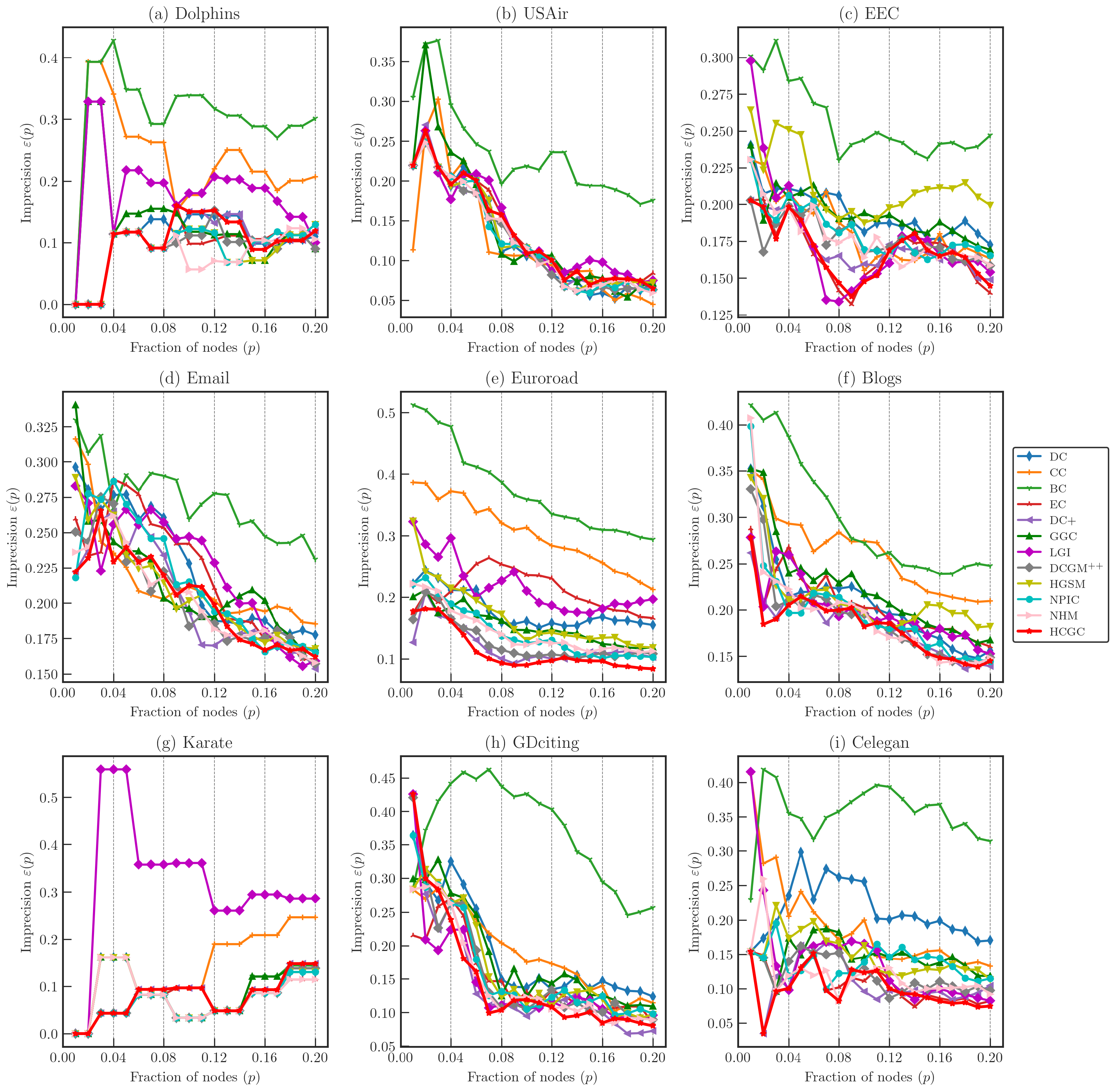
Figure 5.
Comparison of imprecision function of different measures on public real networks dataset with and .
Figure 5.
Comparison of imprecision function of different measures on public real networks dataset with and .
Figure 6.
The nodes in province network with their province labels and communities.
Figure 6.
The nodes in province network with their province labels and communities.
Figure 7.
The nodes of top 20% in province network with their province labels and communities.
Figure 7.
The nodes of top 20% in province network with their province labels and communities.
Figure 8.
The nodes in the district network with their district labels and communities.
Figure 8.
The nodes in the district network with their district labels and communities.
Figure 9.
The nodes in the first community which contains the vital hubs in the network.
Figure 9.
The nodes in the first community which contains the vital hubs in the network.
Table 1.
The name, type, and description for each network in public real networks dataset.
Table 1.
The name, type, and description for each network in public real networks dataset.
| Network | Type | Description |
|---|
| Dolphins | Social | Bottlenose dolphin social interactions in New Zealand waters |
| USAir | Transportation | Undirected transportation network representing the US Air route system from 1997 |
| EEC | Communication | European researchers exchange of emails |
| Email | Communication | Email communication network where users send emails and communicate with each other |
| Euroroad | Transportation | European road network system spanning multiple countries |
| Blogs | Social | A communication network of blogs |
| Karate | Social | Social network of friendships between 34 members of a karate club at a US university in the 1970s. |
| GDciting | Communication | A network of meeting articles that appeared in 1994–2000 |
| Celegan | Biological | Caenorhabditis elegans molecular interaction networks |
Table 2.
Basic properties of public real networks, including number of nodes (N), edges (E), average degree (), shortest path length (), clustering coefficient (), and epidemic threshold ().
Table 2.
Basic properties of public real networks, including number of nodes (N), edges (E), average degree (), shortest path length (), clustering coefficient (), and epidemic threshold ().
| Network | N | E | | | | |
|---|
| Dolphins | 62 | 159 | 5.129 | 3.357 | 0.259 | 0.172 |
| USAir | 332 | 2126 | 12.807 | 2.738 | 0.625 | 0.023 |
| EEC | 986 | 16,064 | 32.584 | 2.587 | 0.407 | 0.014 |
| Email | 1133 | 5451 | 9.622 | 3.606 | 0.220 | 0.057 |
| Euroroad | 1174 | 1417 | 2.414 | 2.418 | 0.017 | 0.500 |
| Blogs | 1222 | 16,714 | 27.355 | 2.738 | 0.320 | 0.012 |
| Karate | 34 | 78 | 4.588 | 2.408 | 0.571 | 0.148 |
| GDciting | 259 | 640 | 4.942 | 1.525 | 0.230 | 0.144 |
| Celegan | 248 | 468 | 3.774 | 1.580 | 0.071 | 0.208 |
Table 3.
List of 77 provinces with corresponding coordinates of their central location.
Table 3.
List of 77 provinces with corresponding coordinates of their central location.
| Order | Province | Latitude | Longitude |
|---|
| 0 | Bangkok | 13.765171 | 100.539168 |
| 1 | Samut Prakan | 13.600400 | 100.597082 |
| ⋮ | ⋮ | ⋮ | ⋮ |
| 76 | Narathiwat | 6.425175 | 101.823515 |
Table 4.
List of 357 adjacent province pairs.
Table 4.
List of 357 adjacent province pairs.
| Order | Origin | Destination |
|---|
| 0 | Bangkok | Samut Prakan |
| 1 | Bangkok | Nonthaburi |
| ⋮ | ⋮ | ⋮ |
| 357 | Narathiwat | Yala |
Table 5.
Adjacency matrix illustrating the connectivity between provinces such as Bangkok, Samut Prakan, and Narathiwat.
Table 5.
Adjacency matrix illustrating the connectivity between provinces such as Bangkok, Samut Prakan, and Narathiwat.
| | Bangkok | Samut Prakan | … | Narathiwat |
|---|
| Bangkok | 0 | 1 | … | 0 |
| Samut Prakan | 1 | 0 | … | 0 |
| ⋮ | ⋮ | ⋮ | ⋮ | ⋮ |
| Narathiwat | 0 | 0 | … | 0 |
Table 6.
List of districts in Thailand along with the geographic coordinates (latitude and longitude) of their central locations.
Table 6.
List of districts in Thailand along with the geographic coordinates (latitude and longitude) of their central locations.
| Order | District Tuple | Latitude | Longitude |
|---|
| 0 | (Phra Nakhon, Bangkok) | 13.765096 | 100.499357 |
| 1 | (Dusit, Bangkok) | 13.777345 | 100.520936 |
| ⋮ | ⋮ | ⋮ | ⋮ |
| 927 | (Cho-airong, Narathiwat) | 6.225381 | 101.811457 |
Table 7.
Lists pairs of adjacent districts, detailing each origin-destination relationship to showcase the direct geographic or administrative connectivity between districts.
Table 7.
Lists pairs of adjacent districts, detailing each origin-destination relationship to showcase the direct geographic or administrative connectivity between districts.
| Order | Origin | Destination |
|---|
| 0 | (Mae Sariang, Mae Hong Son) | (Hot, Chiang Mai) |
| 1 | (Mae Sariang, Mae Hong Son) | (Omkoi, Chiang Mai) |
| ⋮ | ⋮ | ⋮ |
| 6191 | (Wang Sombun, Sa Kaeo) | (Soi Dao, Chanthaburi) |
Table 8.
Adjacency matrix for districts in Thailand, where a 1 indicates direct adjacency between districts and a 0 denotes no adjacency.
Table 8.
Adjacency matrix for districts in Thailand, where a 1 indicates direct adjacency between districts and a 0 denotes no adjacency.
| | (Phra Nakhon, Bangkok) | (Dusit, Bangkok) | … | (Cho-airong, Narathiwat) |
|---|
| (Phra Nakhon, Bangkok) | 0 | 1 | … | 0 |
| (Dusit, Bangkok) | 1 | 0 | … | 0 |
| ⋮ | ⋮ | ⋮ | ⋮ | ⋮ |
| (Cho-airong, Narathiwat) | 0 | 0 | … | 0 |
Table 9.
Basic properties of the province and district networks in the ThaiNet dataset, including number of nodes (N), edges (E), average degree (), shortest path length (), clustering coefficient (), and epidemic threshold ().
Table 9.
Basic properties of the province and district networks in the ThaiNet dataset, including number of nodes (N), edges (E), average degree (), shortest path length (), clustering coefficient (), and epidemic threshold ().
| Network | N | E | | | | |
|---|
| Province | 77 | 179 | 4.649 | 5.586 | 0.505 | 0.230 |
| District | 928 | 3057 | 6.588 | 16.594 | 0.491 | 0.149 |
Table 10.
The Kendall’s correlation coefficient of different measures over public real networks. Where and for a truncation radius. The measure with highest accuracy for each network is highlighted in bold and the measure with the second best is underlined.
Table 10.
The Kendall’s correlation coefficient of different measures over public real networks. Where and for a truncation radius. The measure with highest accuracy for each network is highlighted in bold and the measure with the second best is underlined.
| Network | DC | CC | BC | EC | DC+ | GGC | LGI | DCGM++ | HSGM | NPIC | NHM | HCGC |
|---|
| Dolphins | 0.8274 | 0.6260 | 0.5590 | 0.6587 | 0.8765 | 0.7963 | 0.7984 | 0.9148 | 0.8566 | 0.8661 | 0.8619 | 0.9074 |
| USAir | 0.7679 | 0.8008 | 0.5758 | 0.8803 | 0.8900 | 0.7471 | 0.8517 | 0.8966 | 0.7886 | 0.8068 | 0.8721 | 0.8922 |
| EEC | 0.8524 | 0.8504 | 0.7254 | 0.9042 | 0.9052 | 0.8404 | 0.8577 | 0.9007 | 0.7648 | 0.8699 | 0.8969 | 0.9058 |
| Email | 0.8000 | 0.8079 | 0.6421 | 0.8634 | 0.8937 | 0.8077 | 0.8517 | 0.8873 | 0.8653 | 0.8326 | 0.8955 | 0.9067 |
| Euroroad | 0.6217 | 0.5933 | 0.4173 | 0.5901 | 0.8217 | 0.7799 | 0.7729 | 0.8193 | 0.6967 | 0.7690 | 0.7944 | 0.8662 |
| Blogs | 0.8603 | 0.7814 | 0.6797 | 0.8584 | 0.8889 | 0.8123 | 0.8454 | 0.8979 | 0.7169 | 0.8759 | 0.8893 | 0.9018 |
| Karate | 0.7890 | 0.7505 | 0.6573 | 0.8441 | 0.8146 | 0.7226 | 0.7178 | 0.9198 | 0.8667 | 0.8477 | 0.9064 | 0.8825 |
| GDciting | 0.7686 | 0.7777 | 0.5505 | 0.8263 | 0.9099 | 0.7727 | 0.8453 | 0.9051 | 0.8636 | 0.8410 | 0.9036 | 0.9241 |
| Celegan | 0.7246 | 0.8182 | 0.5462 | 0.8069 | 0.8664 | 0.8022 | 0.7958 | 0.867 | 0.8687 | 0.8225 | 0.8870 | 0.9118 |
Table 11.
The Kendall’s correlation coefficient of different measures over public real networks. Where and for a truncation radius. The measure with highest accuracy for each network is highlighted in bold and the measure with the second best is underlined.
Table 11.
The Kendall’s correlation coefficient of different measures over public real networks. Where and for a truncation radius. The measure with highest accuracy for each network is highlighted in bold and the measure with the second best is underlined.
| Network | DC | CC | BC | EC | DC+ | GGC | LGI | DCGM++ | HSGM | NPIC | NHM | HCGC |
|---|
| Dolphins | 0.8274 | 0.6260 | 0.5590 | 0.6587 | 0.8765 | 0.7709 | 0.7984 | 0.9148 | 0.8566 | 0.8661 | 0.8619 | 0.9000 |
| USAir | 0.7679 | 0.8008 | 0.5758 | 0.8803 | 0.8900 | 0.7077 | 0.8517 | 0.8964 | 0.7886 | 0.8068 | 0.8866 | 0.8956 |
| EEC | 0.8524 | 0.8504 | 0.7254 | 0.9042 | 0.9052 | 0.8226 | 0.8577 | 0.8985 | 0.7648 | 0.8699 | 0.8969 | 0.9038 |
| Email | 0.8000 | 0.8079 | 0.6421 | 0.8634 | 0.8937 | 0.7770 | 0.8517 | 0.8804 | 0.8653 | 0.8326 | 0.8898 | 0.8989 |
| Euroroad | 0.6217 | 0.5933 | 0.4173 | 0.5901 | 0.8217 | 0.8167 | 0.7729 | 0.8389 | 0.6967 | 0.7690 | 0.8060 | 0.8833 |
| Blogs | 0.8603 | 0.7814 | 0.6797 | 0.8584 | 0.8889 | 0.7911 | 0.8454 | 0.8970 | 0.7169 | 0.8759 | 0.8949 | 0.9012 |
| Karate | 0.7890 | 0.7505 | 0.6573 | 0.8441 | 0.8146 | 0.7034 | 0.7178 | 0.9126 | 0.8667 | 0.8477 | 0.8955 | 0.8982 |
| GDciting | 0.7686 | 0.7777 | 0.5505 | 0.8263 | 0.9099 | 0.7593 | 0.8453 | 0.9089 | 0.8636 | 0.8410 | 0.9095 | 0.9226 |
| Celegan | 0.7246 | 0.8182 | 0.5462 | 0.8069 | 0.8664 | 0.8095 | 0.7958 | 0.8776 | 0.8687 | 0.8225 | 0.9038 | 0.9137 |
Table 12.
Imprecision function of different measures over public real networks, where for a truncation radius. The measure with highest accuracy for each network is highlighted in bold and the measure with the second best is underlined.
Table 12.
Imprecision function of different measures over public real networks, where for a truncation radius. The measure with highest accuracy for each network is highlighted in bold and the measure with the second best is underlined.
| Network | DC | CC | BC | EC | DC+ | GGC | LGI | DCGM++ | HSGM | NPIC | NHM | HCGC |
|---|
| Dolphins | 0.1031 | 0.2322 | 0.3082 | 0.0932 | 0.1022 | 0.1326 | 0.1829 | 0.0909 | 0.0863 | 0.0908 | 0.0810 | 0.1007 |
| USAir | 0.1250 | 0.1226 | 0.2358 | 0.1351 | 0.1293 | 0.1385 | 0.1389 | 0.1247 | 0.1286 | 0.1262 | 0.1275 | 0.1340 |
| EEC | 0.1944 | 0.1829 | 0.2567 | 0.1681 | 0.1714 | 0.1931 | 0.1760 | 0.1764 | 0.2132 | 0.1815 | 0.1779 | 0.1683 |
| Email | 0.2254 | 0.2154 | 0.2734 | 0.2208 | 0.2037 | 0.2147 | 0.2240 | 0.2038 | 0.2094 | 0.2151 | 0.2034 | 0.2030 |
| Euroroad | 0.1787 | 0.3034 | 0.3750 | 0.2104 | 0.1208 | 0.1535 | 0.2176 | 0.1272 | 0.1685 | 0.1430 | 0.1437 | 0.1127 |
| Blogs | 0.2093 | 0.2606 | 0.2987 | 0.2044 | 0.1836 | 0.2243 | 0.2002 | 0.1922 | 0.2132 | 0.1970 | 0.1937 | 0.1823 |
| Karate | 0.0812 | 0.1317 | 0.0708 | 0.0883 | 0.0783 | 0.0876 | 0.3177 | 0.0646 | 0.0812 | 0.0635 | 0.0635 | 0.0783 |
| GDciting | 0.1911 | 0.1897 | 0.3679 | 0.1512 | 0.1458 | 0.1812 | 0.1455 | 0.1600 | 0.1656 | 0.1626 | 0.1476 | 0.1484 |
| Celegan | 0.2128 | 0.1915 | 0.3551 | 0.1058 | 0.1095 | 0.1471 | 0.1433 | 0.1206 | 0.1487 | 0.1374 | 0.1193 | 0.0991 |
Table 13.
Imprecision function of different measures over public real networks, where for a truncation radius. The measure with highest accuracy for each network is highlighted in bold and the measure with the second best is underlined.
Table 13.
Imprecision function of different measures over public real networks, where for a truncation radius. The measure with highest accuracy for each network is highlighted in bold and the measure with the second best is underlined.
| Network | DC | CC | BC | EC | DC+ | GGC | LGI | DCGM++ | HSGM | NPIC | NHM | HCGC |
|---|
| Dolphins | 0.1031 | 0.2322 | 0.3082 | 0.0932 | 0.1022 | 0.1381 | 0.1829 | 0.0863 | 0.0863 | 0.0908 | 0.0810 | 0.0977 |
| USAir | 0.1250 | 0.1226 | 0.2358 | 0.1351 | 0.1293 | 0.1372 | 0.1389 | 0.1247 | 0.1286 | 0.1262 | 0.1282 | 0.1340 |
| EEC | 0.1944 | 0.1829 | 0.2567 | 0.1681 | 0.1714 | 0.1932 | 0.1760 | 0.1764 | 0.2132 | 0.1815 | 0.1770 | 0.1683 |
| Email | 0.2254 | 0.2154 | 0.2734 | 0.2208 | 0.2037 | 0.2177 | 0.2240 | 0.2072 | 0.2094 | 0.2151 | 0.2061 | 0.2058 |
| Euroroad | 0.1787 | 0.3034 | 0.3750 | 0.2104 | 0.1208 | 0.1444 | 0.2176 | 0.1238 | 0.1685 | 0.1430 | 0.1399 | 0.1091 |
| Blogs | 0.2093 | 0.2606 | 0.2987 | 0.2044 | 0.1836 | 0.2249 | 0.2002 | 0.1939 | 0.2132 | 0.1970 | 0.1917 | 0.1831 |
| Karate | 0.0812 | 0.1317 | 0.0708 | 0.0883 | 0.0783 | 0.0876 | 0.3177 | 0.0646 | 0.0812 | 0.0635 | 0.0788 | 0.0766 |
| GDciting | 0.1911 | 0.1897 | 0.3679 | 0.1512 | 0.1458 | 0.1903 | 0.1455 | 0.1588 | 0.1656 | 0.1626 | 0.1492 | 0.1474 |
| Celegan | 0.2128 | 0.1915 | 0.3551 | 0.1058 | 0.1095 | 0.1660 | 0.1433 | 0.1242 | 0.1487 | 0.1374 | 0.1151 | 0.1014 |
Table 14.
Imprecision function average of different measures over public real networks, where and for a truncation radius. The measure with highest accuracy for each network is highlighted in bold and the measure with the second best is underlined.
Table 14.
Imprecision function average of different measures over public real networks, where and for a truncation radius. The measure with highest accuracy for each network is highlighted in bold and the measure with the second best is underlined.
| Measure | DC | CC | BC | EC | DC+ | GGC | LGI | DCGM++ | HSGM | NPIC | NHM | HCGC |
|---|
| R = 2 | 0.1690 | 0.2033 | 0.2824 | 0.1530 | 0.1383 | 0.1636 | 0.1940 | 0.1400 | 0.1572 | 0.1463 | 0.1414 | 0.1363 |
| R = 3 | 0.1690 | 0.2033 | 0.2824 | 0.1530 | 0.1383 | 0.1666 | 0.1940 | 0.1400 | 0.1572 | 0.1463 | 0.1408 | 0.1359 |
Table 15.
Top 10 provinces in the province network ranked by different measures.
Table 15.
Top 10 provinces in the province network ranked by different measures.
| Rank | DC | CC | BC | EC | HCGC |
|---|
| Node | Score | Node | Score | Node | Score | Node | Score | Node | Province | Region | Score |
|---|
| 1 | 14 | 0.1184 | 6 | 0.2533 | 61 | 0.3211 | 6 | 0.2734 | 6 | Lopburi | Central | 217,858.6 |
| 2 | 28 | 0.1184 | 58 | 0.2476 | 55 | 0.3062 | 18 | 0.2454 | 28 | Khon Kaen | North
eastern | 216,276.7 |
| 3 | 50 | 0.1184 | 47 | 0.2460 | 62 | 0.3046 | 47 | 0.2357 | 18 | Nakhon
Ratchasima | North
eastern | 200,406.2 |
| 4 | 18 | 0.1053 | 4 | 0.2452 | 69 | 0.2874 | 28 | 0.2286 | 47 | Nakhon Sawan | Central | 200,112.5 |
| 5 | 6 | 0.1053 | 50 | 0.2452 | 67 | 0.2293 | 54 | 0.2258 | 54 | Phetchabun | Northern | 191,681.5 |
| 6 | 47 | 0.1053 | 56 | 0.2428 | 50 | 0.2164 | 4 | 0.2182 | 50 | Tak | Northern | 172,389.4 |
| 7 | 40 | 0.0921 | 9 | 0.2397 | 28 | 0.1930 | 9 | 0.1897 | 4 | Phra Nakhon
Si Ayutthaya | Central | 152,853.1 |
| 8 | 57 | 0.0921 | 48 | 0.2397 | 56 | 0.1929 | 57 | 0.1883 | 16 | Nakhon Nayok | Central | 133,072.0 |
| 9 | 54 | 0.0921 | 18 | 0.2397 | 58 | 0.1702 | 16 | 0.1863 | 58 | Nakhon Pathom | Central | 130,613.8 |
| 10 | 4 | 0.0921 | 54 | 0.2390 | 18 | 0.1637 | 3 | 0.1822 | 9 | Saraburi | Central | 127,022.9 |
Table 16.
Top 10 districts in the district network ranked by different measures.
Table 16.
Top 10 districts in the district network ranked by different measures.
| Rank | DC | CC | BC | EC | HCGC |
|---|
| Node | Score | Node | Score | Node | Score | Node | Score | Node | District | Province | Score |
|---|
| 1 | 14 | 0.0216 | 127 | 0.0861 | 776 | 0.2728 | 6 | 0.2537 | 6 | Pathum Wan | Bangkok | 1.110 |
| 2 | 1 | 0.0205 | 340 | 0.0854 | 777 | 0.2695 | 14 | 0.2503 | 14 | Thon Buri | Bangkok | 1.093 |
| 3 | 6 | 0.0194 | 101 | 0.0852 | 771 | 0.2681 | 1 | 0.2401 | 1 | Dusit | Bangkok | 1.076 |
| 4 | 0 | 0.0183 | 183 | 0.0851 | 770 | 0.2667 | 0 | 0.2337 | 27 | Sa Thon | Bangkok | 9.467 |
| 5 | 27 | 0.0183 | 705 | 0.0849 | 772 | 0.2653 | 12 | 0.2328 | 3 | Bang Rak | Bangkok | 9.421 |
| 6 | 32 | 0.0173 | 118 | 0.0847 | 773 | 0.2638 | 27 | 0.2317 | 0 | Phra Nakhon | Bangkok | 9.341 |
| 7 | 53 | 0.0173 | 203 | 0.0847 | 774 | 0.2624 | 3 | 0.2299 | 12 | Samphanthawong | Bangkok | 8.930 |
| 8 | 12 | 0.0173 | 709 | 0.0844 | 844 | 0.2567 | 17 | 0.2276 | 17 | Khlong San | Bangkok | 8.745 |
| 9 | 24 | 0.0173 | 215 | 0.0841 | 841 | 0.2531 | 7 | 0.2115 | 24 | Bang Phlat | Bangkok | 7.736 |
| 10 | 38 | 0.0173 | 216 | 0.0840 | 769 | 0.2479 | 30 | 0.1989 | 30 | Bang Kho Laem | Bangkok | 7.590 |


 ,
, 


