Crude Oil and Hot-Rolled Coil Futures Price Prediction Based on Multi-Dimensional Fusion Feature Enhancement

Abstract

To address the challenges in forecasting crude oil and hot-rolled coil futures prices, the aim is to transcend the constraints of conventional approaches. This involves effectively predicting short-term price fluctuations, developing quantitative trading strategies, and modeling time series data. The goal is to enhance prediction accuracy and stability, thereby supporting decision-making and risk management in financial markets. A novel approach, the multi-dimensional fusion feature-enhanced (MDFFE) prediction method has been devised. Additionally, a data augmentation framework leveraging multi-dimensional feature engineering has been established. The technical indicators, volatility indicators, time features, and cross-variety linkage features are integrated to build a prediction system, and the lag feature design is used to prevent data leakage. In addition, a deep fusion model is constructed, which combines the temporal feature extraction ability of the convolution neural network with the nonlinear mapping advantage of an extreme gradient boosting tree. With the help of a three-layer convolution neural network structure and adaptive weight fusion strategy, an end-to-end prediction framework is constructed. Experimental results demonstrate that the MDFFE model excels in various metrics, including mean absolute error, root mean square error, mean absolute percentage error, coefficient of determination, and sum of squared errors. The mean absolute error reaches as low as 0.0068, while the coefficient of determination can be as high as 0.9970. In addition, the significance and stability of the model performance were verified by statistical methods such as a paired t-test and ANOVA analysis of variance. This MDFFE algorithm offers a robust and practical approach for predicting commodity futures prices. It holds significant theoretical and practical value in financial market forecasting, enhancing prediction accuracy and mitigating forecast volatility.

1. Introduction

In today’s global economic landscape, financial markets are showing a complex and volatile situation, and crude oil and hot-rolled coil futures play an extremely important role as key components in the field of commodity derivatives [1]. Their price fluctuations are influenced by many factors, which cover the macroeconomic situation, geopolitical situation, changes in supply and demand relations, and market participants’ expectations [2]. It is worth noting that the crude oil and hot-rolled coil future markets do not exist in isolation, and there is a significant economic logic and empirical correlation between them. For example, as an important energy cost, crude oil price directly affects the transportation cost of steel production and the mining cost of raw materials (such as coking coal and iron ore), thus affecting the production cost and market price of hot-rolled coil. On the contrary, as an important industrial sector, the steel industry‘s prosperity will also indirectly affect crude oil demand [3]. This cross-market linkage provides a theoretical basis for using the signal of one market to predict the price of another market. Therefore, accurate prediction of crude oil and hot-rolled coil futures prices is undoubtedly the key to grasping the course in the financial wave for market participants. For investors, accurate price forecasting [4] is the core cornerstone of building a profitable investment strategy, helping them accurately capture the timing of buying and selling, and achieving asset appreciation and preservation. At the same time, effective price forecasting is also an important tool for risk management, helping investors to assess potential risks in advance and allocate assets reasonably [5]. For financial institutions, accurate futures price forecasting is the key basis for optimizing asset allocation and balancing risks and benefits [6], and it helps them to detect abnormal market fluctuations in time and maintain the smooth operation of financial markets [7].

However, the traditional futures price forecasting method [8] exposed many limitations in dealing with the current complex and changeable financial market environment. Traditional models based on statistical analysis [9], such as the linear regression model [10] and auto-regressive moving average model [11], are often based on linear assumptions when dealing with financial data, and it is difficult to capture complex nonlinear relationships that are common in market data [12]. In addition, most of the traditional methods rely on single-dimensional feature analysis, focusing only on the price series itself or individual influencing factors [13], ignoring the multiple dynamics of financial markets [14]. The financial market is a complex system which is intertwined and influenced by many factors. The analysis of a single dimension cannot fully reflect the whole picture of the market, which leads to the lack of sufficient information support for the prediction model and the difficulty of adapting to the rapid changes in the market.

With the rapid development of financial markets and the rapid progress of information technology, the amount of data exploded, and the market put forward higher requirements for futures price forecasting. Today, with the prevalence of high-frequency trading and quantitative investment, investors and financial institutions urgently need models that can accurately predict short-term price fluctuations [15] in order to respond quickly in a rapidly changing market. At the same time, the refined development of quantitative trading strategies has become the key to improving market competitiveness [16]. It is necessary to dig deeper into the potential laws in the data and build more complex and accurate trading strategies. In addition, effective time series data modeling has become an important basis for accurate prediction [17]. This study aims to verify the following hypothesis: the integration of cross-market and multivariate features should significantly improve the accuracy of short-term futures price forecasts. In order to overcome the challenges of existing methods, this study designs a multi-dimensional fusion feature-enhanced (MDFFE) prediction method. The main contributions are as follows:

(1)

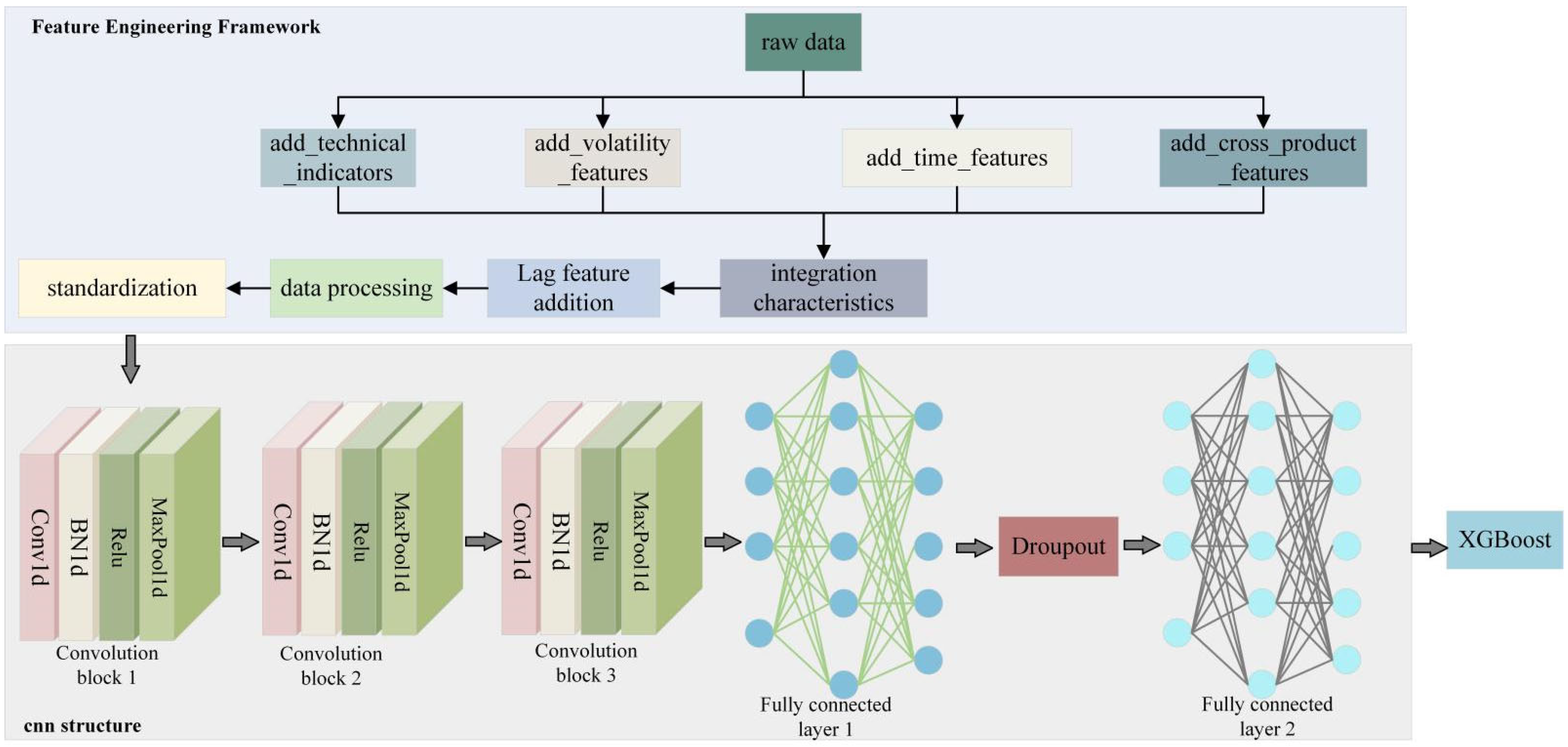
The MDFFE forecasting method is designed to integrate technical indicators, volatility indicators, time characteristics, and cross-species linkage characteristics. This integration aims to uncover hidden information in the data and establish a solid foundation for the futures price forecasting system.

(2)

An innovative lag feature design is implemented, addressing the common issue of data leakage during the model construction phase. This ensures the scientific rigor and dependability of the training process, making it more stringent and standardized. Consequently, it establishes a robust foundation for achieving precise predictions in the future.

(3)

A deep integration of convolutional neural networks (CNN) and extreme gradient boosting (XGBoost) is achieved. By leveraging the strong temporal feature extraction capabilities of CNN and the superior nonlinear mapping of XGBoost, an end-to-end prediction framework is developed. This framework incorporates a meticulously designed three-layer CNN structure and an adaptive weight fusion strategy. It maximizes the strengths of each model while mitigating their weaknesses, significantly enhancing prediction accuracy and reducing variability. This provides a solid basis for the accurate forecasting of futures prices.

2. Related Work

In the domain of predicting crude oil and hot-rolled coil futures prices, numerous researchers conducted comprehensive and detailed studies, yielding various outcomes. However, they still encounter several hurdles and constraints. Early research focused on traditional statistical analysis methods [9]. For example, the linear regression model [10] is widely used to explore the linear relationship between prices and a few macroeconomic variables, trying to predict futures prices by establishing simple linear equations. However, this method oversimplifies the complexity of the market and cannot capture the nonlinear factors behind price changes. The auto-regressive moving average model [11] is designed to forecast future values by leveraging the past data from the price series. Although the characteristics of the time series are considered to a certain extent, it is less adaptable to sudden external shocks and multi-factor interactions in the market.

With the deepening of financial market research, some machine learning methods have been gradually introduced. A support vector machine [18] has certain advantages in dealing with small sample and nonlinear problems and has been used in futures price forecasting. For example, Lang et al. [19] combined fuzzy information granulation with support vector machine to show good results in crude oil futures price forecasting, which effectively improved the prediction accuracy. Zhou et al. [20] used the fusion of Kalman filter and support vector machine to improve the effectiveness of the stock index future investment strategy. Mahmoodi et al. [21] explored the application of a support vector machine in financial time series prediction earlier, which provided a theoretical basis for subsequent research. Kuo et al. [22] optimized the parameters of the support vector machine and improved the accuracy of judging the direction of the stock market. The random forest algorithm [23] predicts by constructing multiple decision trees [24], which can deal with high-dimensional data and have good anti-noise ability. However, it performs poorly in dealing with the long-term dependencies of time series data. Zhao et al. [25] integrated a multi-class classifier and random forest, and the constructed system showed good practicability and effectiveness in financial transaction scenarios. Ping [26] used the random forest regression model to predict the price of treasury bond futures, effectively dealing with high-dimensional data and nonlinear relationships.

In recent years, deep learning methods have begun to emerge in futures price forecasting. Recurrent neural networks (RNN) [27] and their variants of long-short term memory (LSTM) [28] and gated recurrent units (GRU) [29] have been used to deal with the dependency problem of time series data. They can learn the long-term pattern in the price series to a certain extent, but in the face of large-scale and multi-dimensional data, the complexity and computational cost of model training increase sharply, and they are prone to the problem of gradient disappearance or gradient explosion. For example, Pan et al. [30] used the LSTM network to construct a futures price prediction model, which provides a new idea and reference for investors to grasp the futures price trend. Wu et al. [31] integrated multiple factors to predict the futures price of corn and committed to improving the accuracy of prediction. Zhang et al. [32] combined a variational auto-encoder (VAE) with an attention mechanism-improved gated recurrent unit (AMGRU) to construct a more targeted stock index futures price prediction model.

In the feature engineering of financial market forecasting, previous studies often focused on a single type of feature. For example, the research of Wang et al. [33] and Farimani et al. [34] highlighted this limitation, that is, the model’s interpretability is mainly limited to the price behavior itself, and the prediction accuracy is often limited in the face of sudden macroeconomic events or nonlinear market dynamics. Although some studies have begun to consider volatility indicators (such as historical volatility and implied volatility) to reflect market risks and uncertainties, such as the work of Marfatia et al. [35] and Aliu et al. [36]. However, these studies often fail to effectively integrate volatility indicators with the characteristics of other dimensions (such as fundamental data, macroeconomic indicators, cross-market linkage characteristics, or more complex time characteristics), resulting in insufficient information on which the forecasting model is based, and it is difficult to fully reflect the market picture and its inherent complex interactions. In terms of model fusion, although some studies tried to combine different models, the fusion method is relatively simple and fails to give full play to the advantages of each model. For example, Verma et al. [37] used wavelet transform to extract the characteristics of stock market data and input them into a adaptive neuro-fuzzy inference system for prediction. Wang et al. [38] combined the hidden Markov model, artificial neural network, and genetic algorithm to improve the overall performance of the synergy of financial trading systems. Future research can explore more complex fusion strategies in order to make better use of the advantages of different models.

In summary, the existing crude oil and hot-rolled coil futures price forecasting methods have different degrees of limitations in the face of complex and volatile financial markets, whether in the comprehensiveness of feature engineering, the effectiveness of model structures, or the rationality of model fusion. The MDFFE prediction method proposed in this study aims to overcome these limitations and improve the accuracy and stability of futures price prediction through multi-dimensional feature integration, lag feature design, and deep fusion model construction.

3. Multi-Dimensional Fusion Feature-Enhanced Prediction Method

The MDFFE prediction method proposed in this study is shown in Figure 1. Its model architecture consists of two parts: The data enhancement framework of multi-dimensional feature engineering and the deep fusion model. In the data enhancement framework of multi-dimensional feature engineering, starting from the original data, technical indicators, volatility indicators, time characteristics, and cross-variety linkage characteristics are added, respectively. These characteristics can reflect market dynamics, capture market risks, adapt to price volatility cycles, and enrich model information. After adding features, standardization, data processing, and lagging features are added to prevent data leakage and form integrated features. The deep fusion model consists of three parts. The first is a three-layer CNN structure, including convolution blocks 1, 2, and 3. Each layer is composed of convolution, batch normalization, and maximum pooling operations, and gradually extracts multi-scale features from local to global, from short-term to long-term. Then the fully connected layer, including fully connected layers 1 and 2, integrates and maps the features and uses the dropout mechanism to prevent overfitting. Finally, the CNN with strong temporal feature extraction ability and the XGBoost with excellent nonlinear mapping ability are fused by the adaptive weight fusion strategy to achieve efficient prediction.

Table 1. Algorithm model construction process (covering key stages such as data preprocessing, feature engineering, and model construction).

Stages	Step and Method	Description
Data preprocessing and feature engineering	Function: data preprocessing (lookback)
	Extract multi-dimensional features	Includes technical indicators (MA/RSI/MACD/Bollinger Bands), volatility indicators (returns/volatility/amplitude), temporal features (trading session/intra-day minute), and cross-asset linkage features (price ratio/rolling correlation/volume ratio).
	Standardization	Standardize features and target variables to ensure data are on a consistent scale, improving model training efficiency and stability.
	Data splitting	Divide data into training and testing sets based on the given lookback value, ensuring consistent data distribution during model training and testing.
	Returns	Returns training features, training targets, testing features, testing targets, feature scaler, and target scaler.
CNN model construction	Class: CNN model
	Initialize network structure	Define input dimensions, convolutional layers, pooling layers, fully connected layers, and other network structures to build a CNN model for feature extraction and prediction.
	Forward propagation	Input data passes through convolutional layers, activation functions (e.g., ReLU), pooling layers, etc., to extract features and output prediction results.
XGBoost model construction	Class: XGBoost model
	Initialize model	Set hyperparameters, including n_estimators, max_depth, learning_rate, etc., to initialize the XGBoost model for prediction.
	Train	Fit the model using training data to learn the nonlinear mapping relationship between features and target variables.
	Predict	Make predictions on new data and output the prediction results.

lists the construction process of the MDFFE prediction method in detail, covering the key stages of data preprocessing, feature engineering, and model construction, and shows the core steps and methods of each stage and their corresponding descriptions.

3.1. Data Augmentation of Multi-Dimensional Feature Engineering

In the complex and changeable environment of the financial market, it is very important to construct effective feature engineering for futures price prediction. This study proposes an innovative feature engineering framework, as shown in Figure 2, which aims to provide a more accurate and reliable basis for crude oil and hot-rolled coil futures price forecasting through the integration and optimization of multi-dimensional features.

When selecting specific characteristic indicators, we comprehensively consider the theoretical basis, empirical validity of the indicators, and their correlation with the research objectives. For the technical indicators, we selected the classic indicators that have extensive theoretical support in the financial field and have been verified by many empirical studies, such as RSI, which can reflect the state of what is overbought and oversold in the market; the volatility index is selected based on its key role in measuring market uncertainty and risk. For example, yield is an important measure of short-term market volatility, and volatility is the core index in financial risk management. The selection of time characteristics is based on the time periodicity of future market price fluctuation. The determination of cross-variety linkage characteristics stems from the theory that crude oil and hot-rolled coil are related in the macroeconomic environment and industrial chain, and their prices may affect each other. The lag feature design is to prevent data leakage and ensure the reliability and effectiveness of model training.

3.1.1. Technology Index

Technical indicators are statistics calculated based on historical price data. They play an important role in reflecting market trends, trading signals, and price volatility characteristics, and can provide basic market dynamic information for price forecasting.

(1) Relative strength index ($RSI$)

The $RSI$ measures the relative strength of price rises and falls over a period of time. Its calculation formula is as follows:

$$RSI=100-{\displaystyle \frac{100}{1+\frac{AverageGain}{AverageLoss}}}.$$

(1)

Among them, $AverageGain$ is the average value of the increase in the selected time period, and $AverageLoss$ is the average value of the decline in the same period. In the actual calculation, the daily price change value (rise is positive, fall is negative) is usually calculated first, and then the cumulative rise and fall are calculated, respectively, and the average is calculated according to their respective cycles (14 days in this study). Finally, the $RSI$ value is calculated by substituting the above formula. Its value range is usually between 0 and 100. When the $RSI$ value is higher than 70, it indicates that the market is overbought and the price may be called back. When the $RSI$ value is below 30, the market is oversold and the price may rebound. $RSI$ provides investors with a reference to short-term market sentiment by measuring the relative strength of market buying and selling power.

(2) Bollinger bands (BBANDS)

The Bollinger belt is composed of an upper rail, middle rail, and lower rail. The calculation process is as follows:

Middle rail: Typically, this is represented by the moving average; for instance, a 20 day moving average. The computation method aligns with the standard moving average formula mentioned earlier.

$Upper$ rail and $Lower$ rail:

$$UpperBand={MA}_n+k\times \sigma$$

(2)

$$LowerBand={MA}_n-k\times \sigma$$

(3)

where ${MA}_n$ is the daily moving average of $n$ (e.g., $n=20$), $\sigma$ is the standard deviation of the price in the corresponding period, and $k$ is a constant (generally 2).

The fluctuation in the belt’s width can also signal shifts in market volatility. A decrease in the bandwidth might suggest an impending significant price movement. If the price nears the upper boundary, it could indicate that the market is becoming overbought; conversely, if the price approaches the lower boundary, it may suggest that the market is oversold.

3.1.2. Fluctuation Index

Volatility indicators are mainly used to measure the intensity of price fluctuations, which helps to capture market uncertainties and risk factors, thus providing a more comprehensive perspective for price forecasting.

(1) Rate of return

The rate of return evaluates the change in price by determining the percentage shift in the closing value ($Returns$). The formula for this calculation is as follows:

$${Returns}_t={\displaystyle \frac{P_t-P_{t-1}}{P_{t-1}}}.$$

(4)

Here, $P_t$ denotes the closing price for the current period, while $P_{t-1}$ signifies the closing price from the prior period. The return rate effectively captures the extent of price fluctuations and serves as a key metric for assessing short-term market instability. Through examining the dispersion and direction of these returns, we can gain insights into market dynamics and the pace at which prices are shifting.

(2) Volatility

Volatility is determined through the standard deviation of the return rate, employing a sliding window of 20 periods. The formula for this calculation is as follows:

$${Volatility}_t=\sqrt{{\displaystyle \frac{{\sum }_{i=t-19}^t{({Returns}_i-\overline{Returns})}^2}{20}}}.$$

(5)

Among these, ${Returns}_i$ represents the return rate over the $\mathrm{i}$ period, while $Returns$ signifies the mean return rate within a sliding window. Volatility measures the consistency of price movements. Increased volatility implies higher market risk and more drastic price shifts. Conversely, decreased volatility suggests a more stable market. In the realm of financial risk management, volatility serves as a crucial metric for gauging asset risk. For predicting futures prices, variations in volatility can offer insights into the potential range and direction of future price movements.

(3) Amplitude

The amplitude is determined by computing the ratio of the gap between the day’s peak price and its lowest point to the opening value. The formula for this calculation is as follows:

$${Amplitude}_t={\displaystyle \frac{{High}_t-{Low}_t}{{Open}_t}}.$$

(6)

In this context, ${High}_t$ signifies the peak price of the day, ${Low}_t$ denotes the lowest price recorded, and ${Open}_t$ stands for the initial price at the market’s opening. The amplitude serves as a direct indicator of the extent of price variations throughout the day. A more pronounced amplitude suggests significant disparities in prices and heightened trading activity, potentially signaling a shift in the overall market trend or an increase in short-term volatility.

(4) Price interval characteristics

Determine the gap between the maximum and minimum prices (price range) as a feature, with the formula succinctly given by the following:

$${PriceRange}_t={High}_t-{Low}_t.$$

(7)

This aspect resembles amplitude, but zeroes in on the absolute span of price fluctuations, thereby enhancing the volatility measure. It offers a multifaceted view of price variability and supplies additional volatility data for the predictive model.

(5) Trading volume changes

Determine the percentage shift in volume (volume change) using the following formula:

$${VolumeChange}_t={\displaystyle \frac{{Volume}_t-{Volume}_{t-1}}{{Volume}_{t-1}}}.$$

(8)

Here, ${Volume}_t$ signifies the present trading volume, while ${Volume}_{t-1}$ stands for the prior trading volume. Often, a relationship exists between the alteration in trading volume and price movement. For instance, during a price increase, a consistent rise in trading volume might suggest robust bullish momentum, indicating a likely continuation of the upward trend; conversely, if trading volume surges during a price drop, it could signal that bearish forces are in control, potentially leading to a more pronounced downward trend.

3.1.3. Time Characteristics

Given that the price volatility in the future market follows distinct patterns across various time frames, incorporating temporal features can enhance the model’s ability to adjust and grasp these cyclical variations.

(1) Hour and minute characteristics

Retrieve the hour and minute details from the transaction timestamp, which is directly obtained from the transaction time data. It does not involve complex calculations, but only refines the time dimension information to the hour and minute levels. Different trading periods may have different market activity and price fluctuation characteristics. For example, during the period after the opening of the morning session, the market may experience large price fluctuations due to the digestion of overnight information and the influx of new trading orders; at the close of the market, the market trading activity may gradually decrease, and the price fluctuation is relatively small.

(2) Characteristics of the day of the week

The day (day_of_week) is included as a feature, which is also a simple extraction based on transaction time data. It is encoded in the order of the seven days of the week (0 on Monday and 6 on Sunday), because in different trading days of the week, the market may be affected by macroeconomic data releases, industry news, and other factors to show different price movements. For example, some important economic data are usually released on a specific working day, which may lead to large fluctuations in futures prices on that trading day.

(3) Trading period characteristics

Create a binary feature of whether it is morning ($is\_morning$) and whether it is afternoon ($is\_afternoon$), and the calculation formulas are as follows:

$$is\_morning=\left\{\begin{array}{c}1, if 9\le hour<12\\ 0, otherwise\end{array}\right.$$

(9)

$$is\_afternoon=\left\{\begin{array}{c}1, if 13\le hour<15\\ 0, otherwise\end{array}\right..$$

(10)

By differentiating various trading intervals, we can enhance the model’s understanding of market price volatility patterns during distinct time frames. For instance, the composition of market participants, their trading tactics, and the pace of information dissemination might vary between the morning and midday, and these variations will be mirrored in the price movements.

(4) Characteristics of intra-day minute count

To calculate the number of minutes from the opening to the current time ($MinutesfromOpen$), the calculation formula is as follows:

$$MinutesfromOpen=hour\times 60+minute.$$

(11)

This functionality enables the model to grasp the temporal patterns of price variations within a single trading day. For instance, after the market opens, prices might exhibit a distinct rising or falling trajectory, which could shift as the trading session progresses. The intraday minute count serves as a temporal reference point for the model.

3.1.4. Cross-Variety Linkage Characteristics

Crude oil and hot-rolled coil are different types of futures, but they are related to each other in the macroeconomic environment and industrial chain. There may be mutual influence and synergistic change between their prices. Incorporating cross-variety linkage traits can enhance the information input for the predictive model, thereby boosting its flexibility in handling a complex market landscape.

(1) Price ratio characteristics

To calculate the ratio of the closing price of crude oil to hot-rolled coil ($PriceRatio$), the calculation formula is as follows:

$$PriceRatio={\displaystyle \frac{P_{oil}}{P_{rb}}}.$$

(12)

Among them, $P_{oil}$ represents the closing price of crude oil, and $P_{rb}$ represents the closing price of hot-rolled coil. The ratio can reflect the relative strength of the prices of the two varieties. When the price ratio rises, it shows that the price of crude oil rises faster than that of hot-rolled coil. On the contrary, it shows that the price of hot-rolled coil is relatively strong. By monitoring the change in price ratio, we can find the price linkage trend and the change in relative value between the two varieties and provide reference for predicting the price trend.

(2) Rolling correlation characteristics

The rolling window for calculating the yield of crude oil and hot-rolled coil is 20 ($RollingCorr$), and the calculation formula is as follows:

$${RollingCorr}_t=corr\left({Returns}_{oil}\right[t-19:t], {Returns}_{rb}[t-19:t\left]\right).$$

(13)

Among them, ${Returns}_{oil}$ represents the yield sequence of crude oil, ${Returns}_{rb}$ represents the yield sequence of hot-rolled coil, and $corr$ represents the function of calculating the correlation coefficient (such as Pearson correlation coefficient, etc.). The correlation attributes can gauge the level of synchronization in price movements between the two commodities. A high correlation indicates that these commodities exhibit a strong alignment in their price changes, potentially influenced by shared macroeconomic elements or market sentiments. When the correlation is low or changes, it may indicate changes in market structure or influencing factors, which is of great significance for predicting price trends and risk assessment.

(3) Price difference characteristics

To calculate the difference between the closing price of crude oil and hot-rolled coil ($PriceSpread$), the calculation formula is as follows:

$$PriceSpread=P_{oil}-P_{rb}.$$

(14)

The variation in the price gap mirrors the shift in the price discrepancy between the two types. In specific market circumstances, this gap might stay within a defined fluctuation band. Should the gap veer from its typical bounds, it could instigate arbitrage activities, thereby driving the prices back to a balanced state. Consequently, the attributes of this gap are crucial for forecasting price movements and unearthing arbitrage prospects.

(4) Trading volume ratio characteristics

Calculate the $VolumeRatio$ of crude oil to hot-rolled coil. The calculation formula is as follows:

$$VolumeRatio={\displaystyle \frac{{Volume}_{oil}}{{Volume}_{rb}}}.$$

(15)

Among them, ${Volume}_{oil}$ represents the volume of crude oil, and ${Volume}_{rb}$ represents the volume of hot-rolled coil. The trading volume ratio can reflect the relative relationship between the two varieties in the market trading activity. When the volume ratio changes, it may mean that the distribution of market funds between the two varieties changed, which may affect the trend of price fluctuations. For example, if the volume ratio of crude oil rises suddenly, it may indicate that there will be a large price change in the crude oil market.

3.1.5. Lag Feature Design

In order to prevent data leakage and ensure that only historical data are used for calculation and integration in the process of feature construction, this framework adopts lag feature design. Through the lag processing of each feature, the model can only be predicted based on the past information in the training process, so as to avoid misleading the model training due to the early intervention of future information, thus ensuring the timing integrity and reliability of the prediction.

For example, for a certain characteristic $X$ (such as closing price, trading volume, technical indicators and volatility indicators, etc.), the lag characteristic $X_{lag\_i}$ of the $lag\_i$ period ($i$ is a positive integer) is calculated, and the calculation formula is as follows:

$$X_{lag\_i}\left(t\right)=X(t-i).$$

(16)

That is, the value of the feature at time $t-i$ is taken as the lag eigenvalue at time $t$. By setting different lag orders ($lag\_i$, $i$ is the lag order), each feature is lagged. These lag characteristics can offer the evolving trends of past prices and relevant data to the model, aiding it in more effectively grasping the temporal dependencies within price sequences and enhancing the precision of forecasts.

3.2. Deep Fusion Module

In the realm of financial time series prediction, a solitary model frequently struggles to encapsulate the intricate traits and inherent patterns within the data. As depicted in Figure 3, the deep integration component developed here seeks to merge the temporal feature extraction prowess of CNN with the nonlinear modeling strengths of XGBoost, thereby enhancing the precision and reliability of forecasts for crude oil and hot-rolled coil futures prices.

3.2.1. Convolutional Neural Network Structure

This module uses a three-layer CNN structure. In this structure, the convolution layer, batch normalization layer, and pooling layer of each layer work together to gradually extract and optimize feature information. The initial convolutional block employs a one-dimensional convolution with 5 input channels and 64 output channels. The kernel size is set to 3, and the padding is 1. The formula for the convolution operation is as follows:

$$output(n,c_{out}, l)=bias\left(c_{out}\right)+{\sum }_{c_{in}}^{c_{in}}weight(c_{out}, c_{in})\ast input(n, c_{in}, l)$$

(17)

Here, $n$ represents the number of samples, $c_{in}$ and $c_{out}$ represent the number of input and output channels, $l$ represents the length of the sequence, and $\ast$ represents the convolution operation. This configuration enables the convolutional layer to initially extract local feature patterns while preserving the original time series data, such as identifying short-term price fluctuations and the connections between neighboring data points. The formula for the batch normalization layer is as follows:

$${\mu }_B={\displaystyle \frac{1}{m}}{\sum }_{i=1}^m{x}_i , {\sigma }_B^2{\displaystyle \frac{1}{m}}{\sum }_{i=1}^m{{(x}_i-{\mu }_B)}^2, {\widehat{x}}_i={\displaystyle \frac{x_i-{\mu }_B}{\sqrt{{\sigma }_B^2+\epsilon }}}, y_i=\gamma {\widehat{x}}_i+\beta .$$

(18)

Batch normalization is performed on the output of the convolutional layer, where $m$ is the batch size, $x_i$ is the input data, ${\mu }_B$ and ${\sigma }_B^2$ are the batch mean and variance, respectively, $\epsilon$ is a small constant, and $\gamma$ and $\beta$ are learnable parameters. The normalization accelerates training and stabilizes the feature learning process to reduce the impact of changes in data distribution. The pooling layer executes a max pooling operation using a 2 × 2 kernel. It captures the most prominent features within each local region, thereby reducing the data’s dimensionality. This process effectively halves the length of the data sequence, creating a more condensed representation for subsequent feature extraction.

In the second convolutional block, there are 64 input channels and 32 output channels, with a 3 × 3 kernel size and padding of 1. This setup allows for the extraction of more sophisticated and abstract features from the data processed by the preceding layer. As the network deepens, it becomes capable of capturing feature dependencies over longer durations, including medium-term trend shifts in price movements and the interplay between various periodic fluctuations. A batch normalization layer is applied to this convolution’s output to enhance the stability of the training process and boost learning efficiency. Additionally, a max pooling layer with a 2 × 2 kernel is employed, which reduces the dimensionality of the data. Consequently, the length of the data sequence is halved, and the representation of data features becomes increasingly refined.

In the third convolutional block, the input channels for the convolutional layer are 32, while the output channels amount to 16. The convolution kernel is set to a size of 3 with a padding of 1. This configuration continues to refine and integrate the features, extracting more representative and distinctive characteristics. Following the three-layer convolution process, the network can capture multi-scale feature information, ranging from local to global and from short-term to relatively long-term, providing a rich and effective feature input for the subsequent fully connected layer. The batch normalization layer normalizes the convolution output, ensuring stable model training. The pooling layer employs a max pooling approach with a kernel size of 2, halving the data sequence length. After three such pooling operations, the sequence length is reduced to $1/8$, and the final feature map is flattened. The resulting length $16\ast (2101//8)$, where 2101 is a parameter related to the original input data’s sequence length, effectively connects with the fully connected layer, transmitting the extracted multi-scale feature information for further integration and mapping.

The flattened vector is fed into the fully connected layer. As per formula $y=Wx+b$, it is transformed into a 100-dimensional feature space, with $x$ representing the input vector, $W$ the weight matrix, $b$ the bias vector, and $y$ the output vector. Through a combination of global linear and nonlinear transformations, the intricate relationships among features are explored, and deeper insights within the data are extracted, enabling a sophisticated feature representation for the price prediction task. Dropout is applied between the fully connected layers. During training, the outputs of certain neurons are randomly set to zero, which decreases the interdependencies among neurons and mitigates overfitting, allowing the model to learn more robust feature representations and enhancing its predictive performance on unseen data. Finally, formula $y=Wx+b$ is utilized to map the 100-dimensional features to three distinct output channels, corresponding to various prediction goals, such as the price forecast, the classification of price trends, and other objectives, based on the model’s design and application requirements.

3.2.2. Adaptive Weight Fusion Strategy

In order to give full play to the advantages of CNN and XGBoost, an adaptive weight fusion strategy is adopted. Let $y_{CNN}$ be the predictive output of the CNN model and $y_{XGBoost}$ be the predictive output of the XGBoost model. The fused predictive output calculation formula is as follows:

$$y=\alpha y_{CNN}+(1-\alpha )y_{XGBoost}.$$

(19)

Among them, $\alpha$ is the weight of the CNN model, and its value is dynamically adjusted according to the model performance during the training process to meet $0\le \alpha \le 1$. In the early stage of training, CNN quickly extracted basic features, which contributed greatly and relatively high in the process of loss function decline. As the training progresses, XGBoost learns complex nonlinear relationships and increases the impact on prediction accuracy, and the model automatically increases its weight ratio. This strategy avoids the limitation of fixed weight and optimizes the prediction accuracy.

In summary, by constructing a deep fusion module containing a three-layer CNN structure, combining batch normalization and the dropout mechanism, and adopting an adaptive weight fusion strategy, this study successfully combines the temporal feature extraction ability of CNN with the nonlinear mapping advantage of XGBoost to construct an end-to-end prediction framework. The hybrid framework shows excellent performance in the crude oil futures price prediction task. It substantially enhances the precision of forecasts and simultaneously minimizes prediction variability via the integration of multiple models. This approach introduces a novel framework that holds significant theoretical importance and practical relevance for financial market forecasting.

4. Experimental Results and Analysis

4.1. Data Set Introduction

The data set used in this study includes high-frequency trading data of crude oil and hot-rolled coil futures. The time granularity is recorded every 5 min, and the time span is from January 2019 to April 2024. The data set records the core transaction data such as the opening price, the highest price, the lowest price, the closing price, and the trading volume in each 5 min period, which fully reflects the price fluctuation and trading activity of future contracts. The timestamp field accurately records the transaction time of the data, which provides a rich information basis for financial market analysis. The time span of the data set is more than 5 years, covering the price fluctuations of the market under the influence of different economic cycles and events. The characteristics of high-frequency data make the data set particularly suitable for short-term price volatility forecasting tasks, which can capture subtle changes in prices in a short period of time and provide important support for the development of quantitative trading strategies. At the same time, the regular time granularity of data is helpful for constructing an effective time series data model and revealing the inherent law and trend characteristics of price data over time. In order to evaluate the performance of the model, we divide the data set into training set and test set. The training set accounts for 80% of the total data and is used for model training. The test set accounts for 20% of the total data volume and is used to evaluate the generalization ability of the model. This division method ensures the continuity of the training set and the test set in time and simulates the prediction ability of the model for new data in the actual transaction scenario.

4.2. Introduction of Evaluation Index

In this study, the evaluation of the proposed MDFFE model’s effectiveness in forecasting crude oil and hot-rolled coil futures prices is based on several key metrics: mean absolute error (MAE), root mean square error (RMSE), mean absolute percentage error (MAPE), coefficient of determination (R-Squared), and sum of squared errors (SSE). These metrics provide a multidimensional perspective on the accuracy and fit of the model’s predictions compared to actual values, which is crucial for a thorough and detailed performance analysis.

MAE serves to quantify the average absolute difference between the predicted and actual prices. It offers a straightforward measure of the typical deviation in the predictions from the true values. The formula for MAE is as follows:

$$MAE={\displaystyle \frac{1}{n}}{\sum }_{i=1}^n\left|y_i-{\widehat{y}}_i\right|$$

(20)

Among them, $y_i$ represents the real observation value of the $i$ sample, ${\widehat{y}}_i$ represents the model prediction value of the $i$ sample, and $n$ is the number of samples. The smaller the value of MAE is, the smaller the average deviation between the predicted value and the real value of the model is, and the higher the prediction accuracy of the model is.

RMSE serves to quantify the sample standard deviation of the differences between the forecasted and actual values for crude oil and hot-rolled coil futures prices. The formula is as follows:

$$RMSE=\sqrt{{\displaystyle \frac{1}{n}}{\sum }_{i=1}^n{(y_i-{\widehat{y}}_i)}^2}.$$

(21)

RMSE is closely tied to mean squared error (MSE), as it is derived by taking the square root of MSE. This square root operation brings the error back to the same scale as the original data, making it more interpretable in practical contexts. For instance, if futures price data are denominated in a specific currency, the RMSE value indicates the average prediction error per sample in that currency. RMSE takes into account the error across all samples and provides a clear picture of the average deviation between predicted and actual values, complementing MAE to offer a more comprehensive assessment of model accuracy.

MAPE, on the other hand, measures the average percentage error of predictions relative to the actual values, and its formula is as follows:

$$MAPE={\displaystyle \frac{1}{n}}{\sum }_{i=1}^n{\displaystyle \frac{\left|y_i-{\widehat{y}}_i\right|}{y_i}}\times 100\%.$$

(22)

The key benefit of MAPE lies in its ability to neutralize dimensional effects and express prediction errors as percentages. This feature allows for a consistent and straightforward assessment criterion, which is particularly useful when dealing with crude oil and hot-rolled coil futures prices of varying scales or when comparing multiple forecasting models. No matter the scale of the futures prices, MAPE enables a clear comparison of the relative errors from model predictions.

The coefficient of determination, known as R-Squared, is utilized to gauge how well the model fits the data. Its formula is as follows:

$$R-Squared=1-{\displaystyle \frac{{\sum }_{i=1}^n{(y_i-{\widehat{y}}_i)}^2}{{\sum }_{i=1}^n{(y_i-\overline{y})}^2}}$$

(23)

where $\overline{y}$ represents the average of the actual observations. The value of $\mathrm{R}-\mathrm{S}\mathrm{q}\mathrm{u}\mathrm{a}\mathrm{r}\mathrm{e}\mathrm{d}$, when closer to 1, indicates a superior fit of the model to the data, suggesting that the model effectively captures the majority of the data’s variability. Conversely, if B is near 0, the model’s fit is inadequate, potentially due to issues such as an illogical model structure or imprecise parameter estimates, which can lead to unreliable predictions for crude oil and hot-rolled coil futures prices.

SSE quantifies the total squared discrepancy between the predicted and actual values. The formula is as follows:

$$SSE={\sum }_{i=1}^n{y_i-{\widehat{y}}_i}^2.$$

(24)

SSE is centered on the summation of the squared discrepancies between all sample predictions and their actual values. A higher SSE value signifies a greater accumulation of overall prediction errors, indicating that the model’s forecasts significantly diverge from the true values. Conversely, a lower SSE value suggests that the model’s overall prediction deviations are minimal, providing an alternative view of the model’s predictive accuracy.

By thoroughly examining these assessment metrics, the MDFFE model’s effectiveness in forecasting crude oil and hot-rolled coil futures prices can be precisely gauged. This provides a robust foundation for refining and adapting the model, as well as for its practical use in scenarios such as financial market transactions and investment strategies. For instance, investors, financial institutions, and other related entities can leverage these metrics to assess the dependability of the model’s predictions, enabling them to make more informed decisions in futures trading, asset allocation, and risk management, thereby enhancing operational efficiency and performance in financial markets.

4.3. Model Configuration and Theory

To better understand the performance differences among various models, we introduce the models used and their key parameter configurations. These models include BiLSTMModel, CNN, CNNLSTM, LSTM, CNNBiLSTMGRU, TransformerModel, LSTMTransformer, CNNLSTMGRU, and MDFFE. The specific details are shown in

Table 2. Models and their key parameter configurations (detailing each model’s architecture, key parameters, and training methods for comparison and reproducibility).

Model	Description	Key Parameters	Training Method
BiLSTMModel	Bidirectional long short-term memory network, used to capture both forward and backward dependencies.	Input dimension: 2100, hidden layer dimension: 64, output dimension: 1, and number of layers: 1.	Optimizer: Adam, learning rate: 0.001, epochs: 50, batch size: 128, and seed: 666.
CNN	Convolutional neural network, used for feature extraction.	Input channels: 1, output channels: 16, kernel size: 3, and pooling window: 2. Output dimension: 1.	Optimizer: Adam, learning rate: 0.001, epochs: 50, batch size: 128, and seed: 666.
CNNLSTM	A hybrid model combining CNN for feature extraction and LSTM for sequence modeling.	Input dimension: 2100, LSTM hidden layer dimension: 64, output dimension: 1, CNN layers: 2, and LSTM layers: 1.	Optimizer: Adam, learning rate: 0.001, epochs: 50, batch size: 128, and seed: 666.
LSTM	Long short-term memory network, used for processing sequential data.	Input dimension: 2100, hidden layer dimension: 100, number of layers: 5, and output dimension: 1.	Optimizer: Adam, learning rate: 0.001, epochs: 50, batch size: 128, and seed: 666.
CNNBiLSTMGRU	A hybrid model combining CNN, bidirectional LSTM, and GRU layers.	Input dimension: 2100, CNN layers: 2, bidirectional LSTM hidden layer dimension: 64, GRU hidden layer dimension: 64, and output dimension: 1.	Optimizer: Adam, learning rate: 0.001, epochs: 50, batch size: 128, and seed: 666.
TransformerModel	A Transformer-based sequence model.	Input dimension: 2100, embedding dimension: 32, number of layers: 4, attention heads: 8, feed-forward dimension: 128, dropout: 0.1, and output dimension: 1.	Optimizer: Adam, learning rate: 0.001, epochs: 50, batch size: 128, and seed: 666.
LSTMTransformer	A hybrid model combining LSTM and Transformer layers.	Input dimension: 2100, LSTM layers: 4, Transformer layers: 4, embedding dimension: 32, and output dimension: 1.	Optimizer: Adam, learning rate: 0.001, epochs: 50, batch size: 128, and seed: 666.
CNNLSTMGRU	A hybrid model combining CNN, LSTM, and GRU layers.	Input dimension: 2100, CNN layers: 2, LSTM hidden layer dimension: 64, GRU hidden layer dimension: 64, and output dimension: 1.	Optimizer: Adam, learning rate: 0.001, epochs: 50, batch size: 128, and seed: 666.
MDFFE	A hybrid model combining CNN for feature extraction and XGBoost.	CNN output dimension: 128, XGBoost parameters: number of trees: 200, max depth: 10, learning rate: 0.1, weight distribution: CNN 0.2, and XGBoost 0.8.	Optimizer: Adam, learning rate: 0.001, epochs: 50, batch size: 128, and seed: 666.

.

4.4. Quantitative Analyses

Figure 4 shows the comparative experimental results of multiple evaluation indicators through the dot line diagram. In the (a) part, MAE, RMSE, and MAPE indicators show that the MDFFE model performs well, and its corresponding line trend and relative position are significantly lower than other models. This intuitively shows that the MDFFE model has significant advantages in MAE, RMSE, and MAPE. On the contrary, the LSTM model and the LSTMTransformer model perform poorly in these three indicators, and the lines are located at a higher position, indicating that the prediction error is large. The lines of other models, such as BiLSTMModel, CNN, CNNLSTM, CNNBiLSTMGRU, and TransformerModel, are between the two, showing certain predictive ability, but not as good as the MDFFE model. In the R-Squared index of part (b), the lines corresponding to the MDFFE model show that it has an excellent fitting effect on the data and is located at the highest position, which indicates that the model can highly explain the variability of the data. However, the LSTM model and the LSTMTransformer model have a poor fitting effect, and the lines are at a low position. In the SSE index of part (c), the lines of the MDFFE model show that its cumulative error is the smallest and at the lowest position, which again confirms the accuracy and stability of the MDFFE model prediction.

Table 3. Quantitative analysis of comparative experiments (quantitative results of each model on key evaluation indicators are listed for evaluating prediction performance).

Model	MAE↓	RMSE↓	MAPE↓	R-Squared	SSE↓
BiLSTMModel	0.0806	0.0980	0.0842	0.5916	206.7034
CNN	0.0720	0.0838	0.0720	0.7019	150.8885
CNNLSTM	0.1403	0.1957	0.1475	−0.6273	823.6530
LSTM	0.2427	0.3332	0.2592	−3.7164	2387.2202
CNNBiLSTMGRU	0.1314	0.1665	0.1464	−0.1782	596.3677
TransformerModel	0.1395	0.1689	0.1519	−0.2123	613.5961
LSTMTransformer	0.2504	0.2831	0.2813	−2.4046	1723.2487
CNNLSTMGRU	0.1298	0.1751	0.1288	−0.3020	659.0109
MDFFE	0.0068	0.0084	0.0071	0.9970	1.5090

shows the quantitative analysis results of comparative experiments of various models in the crude oil and hot-rolled coil futures price prediction task. These models include BiLSTMModel, CNN, CNNLSTM, LSTM, CNNBiLSTMGRU, TransformerModel, LSTMTransformer, CNNLSTMGRU, and the MDFFE model proposed in this study. The evaluation indicators cover MAE↓, RMSE↓, MAPE↓, R-Squared, and SSE↓. The best results are highlighted in bold.

In the task of crude oil and hot-rolled coil futures price prediction, the MDFFE model shows comprehensive and significant advantages in MAE, RMSE, MAPE, R-Squared, and SSE. The MAE value of the MDFFE model is 0.0068, which is much lower than all other comparison models (e.g., CNN is 0.0720, LSTM is as high as 0.2427), indicating that the MDFFE model has a significant advantage in mean absolute error and high prediction accuracy. In terms of RMSE, the MDFFE model’s 0.0084 is also much lower than other models (e.g., CNN’s 0.0838, LSTM’s 0.3332), reflecting its strong stability. On the MAPE index, the MDFFE model is only 0.0071. After eliminating the influence of dimension, the relative error is very small and the control ability is outstanding. The R-Squared of the MDFFE model is as high as 0.9970, which indicates that the fitting effect of the model on the data is almost perfect. In contrast, the R-Squared value of other models is much lower than that of the MDFFE model, and even negative (such as −0.6273 of CNNLSTM and −3.7164 of LSTM), which indicates that they have a large deficiency in data fitting. From the perspective of error square sum SSE, the MDFFE model is only 1.5090, which is much lower than other models (such as 206.7034 of BiLSTMModel and 150.8885 of CNN), which once again confirms the excellent prediction performance of the MDFFE model.

Figure 5 shows the point-line diagram of the ablation experiment, including the performance of MAE, RMSE, MAPE, R-Squared, and SSE on different model configurations (CNN, CNN-FE, and MDFFE). On the MAE, RMSE, and MAPE indicators, we observed a significant downward trend in the corresponding points from CNN to CNN-FE to MDFFE. This intuitively shows that with the addition of FE and XGBoost-integrated components, the prediction error of the model is gradually reduced, and the prediction accuracy is continuously improved. On the R-Squared index, CNN has the lowest corresponding point, CNN-FE increased, and MDFFE has the highest, which indicates that R-Squared increases significantly with model optimization, confirming the great contribution of feature engineering and model fusion to model fitting ability. In terms of SSE index, CNN has the highest point, CNN-FE decreases, and MDFFE is the lowest, indicating that SSE continues to decrease with the improvement of the model, further verifying the effective reduction in the cumulative error of the model.

Table 4. Quantitative analysis of ablation. The table illustrates the performance variations of different model configurations on key evaluation metrics and validates the effects of feature engineering and model fusion.

CNN	FE	XGBoost	MAE↓	RMSE↓	MAPE↓	R-Squared	SSE↓
√	×	×	0.0720	0.0838	0.0720	0.7019	150.8885
√	√	×	0.0250	0.0376	0.0254	0.9353	44.6601
√	√	√	0.0068	0.0084	0.0071	0.9970	1.5090

shows the quantitative analysis results of ablation under different model settings. The key elements involved include the use of CNN, FE, and XGBoost, and the important evaluation index data of MAE↓, RMSE↓, MAPE↓, R-Squared, and SSE ↓ are presented. The best results are highlighted in bold.

Table 4 clearly shows that as the model components are gradually added, the performance indicators are significantly improved. When CNN is only enabled, MAE is 0.0720, RMSE is 0.0838, MAPE is 0.0720, R-Squared is 0.7019, and SSE is 150.8885. When CNN was enabled and FE was added, the indicators were greatly improved: MAE decreased to 0.0250, RMSE decreased to 0.0376, MAPE was 0.0254, R-Squared increased to 0.9353, and SSE decreased to 44.6601. This fully demonstrates that feature engineering plays a key role in extracting effective information and improving model performance. When the complete MDFFE model (including CNN, FE, and XGBoost) is enabled, the indicators reach the best, MAE is as low as 0.0068, RMSE is 0.0084, MAPE is 0.0071, R-Squared is as high as 0.9970, and SSE is only 1.5090. This shows that XGBoost, as an integrated learning component, further enhances the prediction ability and fitting effect of the model in the MDFFE model. From the perspective of feature engineering and model fusion, MAE, RMSE, and MAPE continue to decrease with the addition of FE and XGBoost, R-Squared continues to increase, and SSE continues to decrease, which clearly shows the gradual optimization of model performance.

4.5. Qualitative Analyses

Figure 6 shows the qualitative analysis results of crude-oil futures prices by multiple models, including BiLSTMModel, CNNModel, CNNLSTMModel, LSTMModel, TransformerModel, and MDFFEModel. Each subgraph clearly presents two curves of ‘real‘ (real value) and ‘pred‘ (predicted value), and intuitively compares the accuracy and stability of each model in predicting crude oil futures prices. Through observation, it is found that although the predicted value of BiLSTMModel has a certain follow-up with the actual value, there are obvious deviations in some areas, indicating that it lacks in capturing details. Compared with the BiLSTMModel, the fit of the CNNModel is improved, but there are still deviations. The fluctuation frequency of CNNLSTMModel is high, showing a certain follow-up, but the deviation phenomenon is still obvious. The predicted value of the LSTMModel deviates significantly from the actual value, and the fluctuation range and frequency are large, indicating that it is difficult to effectively capture the complex fluctuations of futures prices. The fit of TransformerModel is better than that of LSTMModel, but there are still fluctuations in capturing long-term dependence and complex nonlinear relationships. The most noteworthy is that the MDFFE model has the highest degree of fit, its prediction curve almost coincides with the actual value, and the fluctuation amplitude and frequency are the smallest, which intuitively proves that the MDFFE model reached the best level in the accuracy and stability of crude oil futures price prediction.

4.6. Statistical Tests

The mean absolute error of the target model (MDFFE) is 0.002753. This shows that the prediction error of the MDFFE model is very small and the prediction accuracy is very high. Paired t-tests were performed on the MDFFE model and each of the other models to assess whether the difference in error was significant. Mean error difference: The average error difference between the target model and the comparison model. The negative value indicates that the error of the MDFFE model is smaller than that of the comparison model. For example, compared with the BiLSTMModel, the average error difference of the MDFFE model is−0.077870, indicating that the error of the MDFFE model is significantly lower than that of the BiLSTMModel. T-statistic: T-test statistics, the greater the absolute value, the more significant the difference. For example, the t statistic with the BiLSTMModel is −205.316403, indicating a very significant difference. T-test p-value: The p value is 0, indicating that the difference is significant at the significance level of 0.05. The smaller the p value, the more significant the difference. T-test significance (α = 0.05): the significance of all comparison models is ‘Significant’, indicating that the performance of the MDFFE model is significantly better than all other models. The paired t-test results of the models are shown in

Table 5. Paired t-test results of MDFFE model and other models.

Model	Target Model Mean Error	Comparison Model Mean Error	Mean Error Difference	T-Statistic	T-Test p-Value	Wilcoxon Statistic	Wilcoxon p-Value	Cohen d	T-Test Significance (α = 0.05)	Wilcoxon Significance (α = 0.05)
BiLSTMModel	0.002752569	0.08062279	−0.07787022	−205.3164029	0	231,432	0	−2.788792657	Significant	Significant
CNN	0.002752569	0.072012575	−0.069260006	−239.5481362	0	105,285	0	−3.229293133	Significant	Significant
CNNLSTM	0.002752569	0.148733619	−0.145981049	−142.4923388	0	94,251	0	−1.93765241	Significant	Significant
LSTM	0.002752569	0.230479288	−0.227726718	−164.3823637	0	23,563	0	−2.239282064	Significant	Significant
CNNBiLSTMGRU	0.002752569	0.138434251	−0.135681681	−191.5883282	0	26,907	0	−2.586981754	Significant	Significant
TransformerModel	0.002752569	0.127368013	−0.124615444	−226.0726834	0	70,486	0	−3.069560968	Significant	Significant
LSTMTransformer	0.002752569	0.136183782	−0.133431213	−186.1417067	0	65,410	0	−2.513974888	Significant	Significant
CNNLSTMGRU	0.002752569	0.111576971	−0.108824401	−166.9906497	0	116,873	0	−2.252380018	Significant	Significant

.

Figure 7 shows the absolute error distribution of different models by box plot and reveals the difference of prediction accuracy of each model. The box plot comprehensively shows the concentration trend, dispersion degree, and abnormal situation of the data through the box, median line, whisker line, and outliers. The box position of the MDFFE model is the lowest, indicating that the prediction error is the smallest and the data are concentrated. The median line is at the lowest position, which further highlights its prediction accuracy advantage; the number of outliers is small, and the distribution is concentrated, indicating that the prediction stability is high. The models in the figure are arranged in ascending order of average error. The MDFFE model is located on the far left side, with the smallest average error and the highest prediction accuracy. In general, the MDFFE model is significantly superior to other models in terms of prediction accuracy and stability, showing excellent prediction performance.

The results of analysis of variance (ANOVA) in

Table 6. ANOVA analysis of variance results.

Source	sum_sq	df	F	PR (>F)
C (model)	671.944528	8.0	7053.753944	0.0
Residual	2304.543389	193,536.0	NaN	NaN

show that there are significant differences in the mean absolute error between different models. The sum of squares of C (model) is 671.944528, the degree of freedom is 8, the F value is as high as 7053.753944, and the corresponding p value is 0.0. This shows that at the significant level of 0.05, the difference between the models is extremely significant, and the greater the F value, the more significant the difference between the models. The sum of squares of residuals is 2304.543389, and the degree of freedom is 193,536. The residual represents the error inside the model, that is, the difference between the predicted value and the actual value of the model. Although the sum of squares of residuals is large, the difference between models is more significant than the error within the model, which further confirms that there are significant differences in prediction accuracy between different models.

5. Discussions

The MDFFE model proposed in this study achieved excellent performance in the crude oil futures price prediction task, which is manifested in extremely low prediction error (MAE = 0.0068) and an R-Squared value of 0.9970. These results significantly exceed a variety of benchmark models, including BiLSTM, CNN, LSTM, and Transformer variants. We understand that such a high R-Squared value may cause concerns about overfitting in the field of time series prediction, as well as questions about information leakage. In this regard, we ensure the robustness and generalization ability of the model through a number of strategies: First, the model is fully trained on massive historical data, aiming to learn universal laws rather than noise; secondly, the data are strictly and randomly divided into training and test sets, and the consistency and robustness of the performance of the model on different data subsets are verified by experiments with multiple rounds of random seeds. This method effectively simulates the effect of cross-validation. Finally, we strictly eliminate the leakage of any future information in the whole data processing process and ensure the authenticity of the prediction. The excellent performance of the MDFFE model is mainly attributed to its innovative methodology: it comprehensively integrates market dynamic information through fine multi-dimensional feature engineering, especially in that the model can effectively use the feature relationship between crude oil and hot-rolled coil futures data sets to enhance the prediction of crude oil prices. More importantly, it skillfully combines the local pattern capture ability of CNN with the nonlinear modeling and integrated learning advantages of XGBoost. This hybrid architecture forms a strong complementary effect, which significantly improves the prediction accuracy and stability.

Although this study mainly demonstrates the excellent performance of the MDFFE model in crude oil futures price forecasting, we believe that its core design concept and methodology have good universality and scalability, and are expected to show similar excellent performance in other types of futures or asset price forecasting. The reasons are as follows:

The versatility of multi-source data fusion: Our model design can effectively fuse data from different assets to enrich the feature set. Even if the prediction target is a single asset, it can also capture more complex market dynamics by introducing information on related assets. This method can be easily extended to other financial products. For example, when predicting a stock, data such as its industry index and related company’s stock can be included at the same time.

Universality of feature engineering: The multi-dimensional feature engineering methods used in the model (e.g., time series features, technical indicators, and cross-market correlation analysis) have universal predictive value in various financial markets. Whether it is stocks, foreign exchange, bonds, or other commodity futures, their price movements are often affected by similar time, technology, and interrelated factors.

Advantages of the hybrid model: CNN performs well in capturing local features and short-term patterns in a time series, while XGBoost, as a powerful ensemble learning model, is good at dealing with complex nonlinear relationships and high-dimensional data. This combination can effectively extract and learn the deep rules of price changes from different levels. The advantages of this hybrid structure are not limited to the crude oil market. In other financial assets, such as intraday fluctuations in stock prices and trend reversals in the foreign exchange market, there are similar local patterns and complex nonlinear relationships.

The ability to adapt to market fluctuations: Financial markets are generally characterized by high noise, non-linearity, and non-stationarity. The MDFFE model can better cope with these challenges through its robust architecture and feature engineering. As long as the model can extract effective features that reflect its market characteristics, the model has the potential to make effective predictions on different financial products.

In this study, the excellent performance of the MDFFE model was further verified by statistical methods such as a paired t-test and ANOVA analysis of variance. The results of the paired t-test showed that the error difference between the MDFFE model and other comparison models was significant, reaching the significant standard at the significant level (α = 0.05), which proved that its performance was significantly better. ANOVA analysis of variance also showed that there were significant differences in the mean absolute error between different models, which further highlighted the excellent performance of the MDFFE model. Although the MDFFE model performs well in existing tasks, we still recognize its limitations, including the ability to extrapolate on other financial products to be verified and the dependence on artificial engineering features. Future research will focus on quantifying model performance differences through statistical significance tests, conducting more detailed performance analysis under different market conditions, and exploring ways to enhance model interpretability.

6. Conclusions

In summary, this study successfully developed and validated the MDFFE model, an innovative solution for accurate prediction of commodity futures prices. The performance of the model on the data set of crude oil and hot-rolled coil futures proves its extremely high prediction accuracy and fitting ability, which is reflected in the indicators such as the MAE as low as 0.0068 and R-Squared as high as 0.9970. Its comprehensive performance is significantly better than the existing mainstream deep learning prediction model. The success of the MDFFE model is mainly due to its core innovation—the deep fusion of multi-dimensional features and the organic combination of CNN and XGBoost-integrated learning, which enables it to efficiently capture nonlinear patterns and multi-dimensional dependencies in a complex financial time series. Through large-scale data training, strict random data partitioning, and multiple rounds of experiments, we ensure the robustness and generalization ability of the model results and effectively deal with the potential risk of overfitting and information leakage. The MDFFE model provides an efficient and reliable futures price forecasting tool for financial markets, which has important theoretical and practical value. Although the current research still has limitations, such as cross-product extrapolation ability and dependence on engineering characteristics, we are confident in its future development potential and clarified the follow-up research direction, aiming to further improve the universality, interpretability, and adaptability of the model in complex market environments.

References

1. Liu, Y.; Li, H.; Ren, H.; Jiang, H.; Ren, B.; Ma, N.; Chen, Z.; Zhong, W.; Ulgiati, S. Shared responsibility for carbon emission reduction in worldwide “steel-electric vehicle” trade within a sustainable industrial chain perspective. Ecol. Econ. 2025, 227, 108393. [Google Scholar] [CrossRef]
2. Chen, X.; Tongurai, J. Revisiting the interdependences across global base metal futures markets: Evidence during the main waves of the COVID-19 pandemic. Res. Int. Bus. Financ. 2024, 70, 102391. [Google Scholar] [CrossRef]
3. Krekel, G.; Suer, J.; Traverso, M. Identifying the social hotspots of German steelmaking and its value chain. Sustain. Prod. Consum. 2024, 51, 222–235. [Google Scholar] [CrossRef]
4. Derakhshani, R.; GhasemiNejad, A.; Amani Zarin, N.; Amani Zarin, M.M.; Jalaee, M.S. Forecasting copper prices using deep learning: Implications for energy sector economies. Mathematics 2024, 12, 2316. [Google Scholar] [CrossRef]
5. Mensi, W.; Aslan, A.; Vo, X.V.; Kang, S.H. Time-frequency spillovers and connectedness between precious metals, oil futures and financial markets: Hedge and safe haven implications. Int. Rev. Econ. Financ. 2023, 83, 219–232. [Google Scholar] [CrossRef]
6. Kumar, S.; Kumar, A.; Singh, G. Causal relationship among international crude oil, gold, exchange rate, and stock market: Fresh evidence from NARDL testing approach. Int. J. Financ. Econ. 2023, 28, 47–57. [Google Scholar] [CrossRef]
7. Fiszeder, P.; Fałdziński, M.; Molnár, P. Attention to oil prices and its impact on the oil, gold and stock markets and their covariance. Energy Econ. 2023, 120, 106643. [Google Scholar] [CrossRef]
8. Ben Ameur, H.; Boubaker, S.; Ftiti, Z.; Louhichi, W.; Tissaoui, K. Forecasting commodity prices: Empirical evidence using deep learning tools. Ann. Oper. Res. 2024, 339, 349–367. [Google Scholar] [CrossRef]
9. Zurakowski, D.; Staffa, S.J. Statistical power and sample size calculations for time-to-event analysis. J. Thorac. Cardiovasc. Surg. 2023, 166, 1542–1547.e1. [Google Scholar] [CrossRef]
10. Rios-Avila, F.; Maroto, M.L. Moving beyond linear regression: Implementing and interpreting quantile regression models with fixed effects. Sociol. Methods Res. 2024, 53, 639–682. [Google Scholar] [CrossRef]
11. Xu, L.; Xu, H.; Ding, F. Adaptive multi-innovation gradient identification algorithms for a controlled autoregressive autoregressive moving average model. Circuits Syst. Signal Process. 2024, 43, 3718–3747. [Google Scholar] [CrossRef]
12. Shyu, Y.W.; Chang, C.C. A hybrid model of memd and pso-lssvr for steel price forecasting. Int. J. Eng. Manag. Res. 2022, 12, 30–40. [Google Scholar] [CrossRef]
13. Wu, S.; Wang, W.; Song, Y.; Liu, S. An EEMD-LSTM, SVR, and BP decomposition ensemble model for steel future prices forecasting. Expert Syst. 2024, 41, e13672. [Google Scholar] [CrossRef]
14. Li, C.; Wu, C.; Zhou, C. Forecasting equity returns: The role of commodity futures along the supply chain. J. Futures Mark. 2021, 41, 46–71. [Google Scholar] [CrossRef]
15. Khattak, B.H.A.; Shafi, I.; Khan, A.S.; Flores, E.S.; Lara, R.G.; Samad, M.A.; Ashraf, I. A systematic survey of AI models in financial market forecasting for profitability analysis. IEEE Access 2023, 11, 125359–125380. [Google Scholar] [CrossRef]
16. Wang, J.; Zhuang, Z.; Feng, L. Intelligent optimization based multi-factor deep learning stock selection model and quantitative trading strategy. Mathematics 2022, 10, 566. [Google Scholar] [CrossRef]
17. Kontopoulou, V.I.; Panagopoulos, A.D.; Kakkos, I.; Matsopoulos, G.K. A review of ARIMA vs. machine learning approaches for time series forecasting in data driven networks. Future Internet 2023, 15, 255. [Google Scholar] [CrossRef]
18. Roy, A.; Chakraborty, S. Support vector machine in structural reliability analysis: A review. Reliab. Eng. Syst. Saf. 2023, 233, 109126. [Google Scholar] [CrossRef]
19. Lang, G.; Zhao, L.; Miao, D.; Ding, W. Granular-Ball Computing Based Fuzzy Twin Support Vector Machine for Pattern Classification. IEEE Trans. Fuzzy Syst. 2025, 99, 1–13. [Google Scholar] [CrossRef]
20. Zhou, Y.; Wang, S.; Xie, Y.; Zhu, T.; Fernandez, C. An improved particle swarm optimization-least squares support vector machine-unscented Kalman filtering algorithm on SOC estimation of lithium-ion battery. Int. J. Green Energy 2024, 21, 376–386. [Google Scholar] [CrossRef]
21. Mahmoodi, A.; Hashemi, L.; Jasemi, M.; Mehraban, S.; Laliberté, J.; Millar, R.C. A developed stock price forecasting model using support vector machine combined with metaheuristic algorithms. Opsearch 2023, 60, 59–86. [Google Scholar] [CrossRef]
22. Kuo, R.J.; Chiu, T.H. Hybrid of jellyfish and particle swarm optimization algorithm-based support vector machine for stock market trend prediction. Appl. Soft Comput. 2024, 154, 111394. [Google Scholar] [CrossRef]
23. Yin, L.; Li, B.; Li, P.; Zhang, R. Research on stock trend prediction method based on optimized random forest. CAAI Trans. Intell. Technol. 2023, 8, 274–284. [Google Scholar] [CrossRef]
24. Chou, J.S.; Chen, K.E. Optimizing investment portfolios with a sequential ensemble of decision tree-based models and the FBI algorithm for efficient financial analysis. Appl. Soft Comput. 2024, 158, 111550. [Google Scholar] [CrossRef]
25. Zhao, J.; Lee, C.D.; Chen, G.; Zhang, J. Research on the Prediction Application of Multiple Classification Datasets Based on Random Forest Model. In Proceedings of the 2024 IEEE 6th International Conference on Power, Intelligent Computing and Systems (ICPICS), Shenyang, China, 26–28 July 2024; IEEE: New York, NY, USA, 2024; pp. 156–161. [Google Scholar]
26. Ping, W.; Hu, Y.; Luo, L. Price Forecast of Treasury Bond Market Yield: Optimize Method Based on Deep Learning Model. IEEE Access 2024, 12, 194521–194539. [Google Scholar] [CrossRef]
27. Mienye, I.D.; Swart, T.G.; Obaido, G. Recurrent neural networks: A comprehensive review of architectures, variants, and applications. Information 2024, 15, 517. [Google Scholar] [CrossRef]
28. Pathak, D.; Kashyap, R. Neural Correlate-Based E-Learning Validation and Classification Using Convolutional and Long Short-Term Memory Networks. Trait. Du Signal 2023, 40, 1457. [Google Scholar] [CrossRef]
29. Wan, W.D.; Bai, Y.; Lu, Y.N.; Ding, L. A hybrid model combining a gated recurrent unit network based on variational mode decomposition with error correction for stock price prediction. Cybern. Syst. 2024, 55, 1205–1229. [Google Scholar] [CrossRef]
30. Pan, H.; Tang, Y.; Wang, G. A Stock Index Futures Price Prediction Approach Based on the MULTI-GARCH-LSTM Mixed Model. Mathematics 2024, 12, 1677. [Google Scholar] [CrossRef]
31. Wu, B.; Wang, Z.; Wang, L. Interpretable corn future price forecasting with multivariate time series. J. Forecast. 2024, 43, 1575–1594. [Google Scholar] [CrossRef]
32. Zhang, Y.T.; Jin, C.T.; Li, Y. Stock Index Futures Price Prediction Based on VAE-ATTGRU Model. Comput. Eng. Appl. 2024, 60, 293–301. [Google Scholar]
33. Wang, H.C.; Hsiao, W.C.; Liou, R.S. Integrating technical indicators, chip factors and stock news for enhanced stock price predictions: A multi-kernel approach. Asia Pac. Manag. Rev. 2024, 29, 292–305. [Google Scholar] [CrossRef]
34. Farimani, S.A.; Jahan, M.V.; Fard, A.M.; Tabbakh, S.R.K. Investigating the informativeness of technical indicators and news sentiment in financial market price prediction. Knowl.-Based Syst. 2022, 247, 108742. [Google Scholar] [CrossRef]
35. Marfatia, H.A.; Ji, Q.; Luo, J. Forecasting the volatility of agricultural commodity futures: The role of co-volatility and oil volatility. J. Forecast. 2022, 41, 383–404. [Google Scholar] [CrossRef]
36. Aliu, F.; Asllani, A.; Hašková, S. The impact of bitcoin on gold, the volatility index (VIX), and dollar index (USDX): Analysis based on VAR, SVAR, and wavelet coherence. Stud. Econ. Financ. 2024, 41, 64–87. [Google Scholar] [CrossRef]
37. Verma, S.; Sahu, S.P.; Sahu, T.P. Discrete wavelet transform-based feature engineering for stock market prediction. Int. J. Inf. Technol. 2023, 15, 1179–1188. [Google Scholar] [CrossRef]
38. Wang, B. A research on resistance spot welding quality judgment of stainless steel sheets based on revised quantum genetic algorithm and hidden markov model. Mech. Syst. Signal Process. 2025, 223, 111881. [Google Scholar] [CrossRef]
Figure 1. MDFFE model architecture diagram (the construction process of MDFFE method is listed in detail, covering the key stages of data preprocessing, feature engineering, and model construction).
Algorithms 18 00357 g001
Figure 2. Multi-dimensional feature engineering diagram (shows the multi-dimensional feature engineering framework, covering the design and integration of technical indicators, volatility indicators, time characteristics, cross-variety linkage characteristics, and lag characteristics).
Algorithms 18 00357 g002
Figure 3. Deep fusion module diagram (shows the architecture of CNN and XGBoost fusion, highlighting its synergistic advantages in time series feature extraction and nonlinear mapping).
Algorithms 18 00357 g003
Figure 4. The experimental point line diagram (shows the performance comparison of different models on multiple evaluation indicators, including MAE, RMSE, MAPE, R-Squared, and SSE).
Algorithms 18 00357 g004
Figure 5. The ablation experiment point line diagram (shows the performance changes of different model configurations on key evaluation indicators and verifies the effect of feature engineering and model fusion).
Algorithms 18 00357 g005
Figure 6. Comparison of Fitting Performance. Figure Show the fitting of the actual and predicted values of crude oil futures prices by different models and intuitively compares the prediction accuracy and stability of each model.
Algorithms 18 00357 g006aAlgorithms 18 00357 g006b
Figure 7. Box line diagram.
Algorithms 18 00357 g007