4.1. Dataset Preparation
We collected 38,387 and 7993 malicious URL samples from two independent cloud platforms, PhishTank and Any.Run, respectively, along with 205,628 legitimate URLs from DMOZ. Since the number of malicious samples is smaller than the number of legitimate samples, we merged additional data from Any.Run to enhance the malicious dataset. After collecting the datasets, we performed preprocessing steps including removing duplicate links, missing values, null values, and control characters, trimming leading/trailing slashes and whitespace, normalizing URLs to lowercase, and decoding encoded URLs into ASCII characters. Following preprocessing, the legitimate dataset contained 205,628 samples, and the malicious dataset contained 46,380 samples. This imbalance between the two classes could bias the model during training and testing. To address this, we shuffled the datasets by label and performed class balancing through under-sampling, selecting the minimum number of samples from each class to achieve balance. Before proceeding to tokenization and downstream tasks, we validated the dataset using transformation techniques and the interquartile range (IQR) to ensure quality and consistency.
4.2. Dataset Validation
To ensure the quality and appropriateness of our dataset, we implemented the preprocessing techniques and visualized the skewness levels [
23,
24].
Figure 5 shows the distribution of URL lengths in the dataset. The tallest bar falls within the 0–50 character range, indicating a significant concentration of shorter URLs. This suggests that the majority of URLs in the sample are relatively short. Only a small number of URLs exceed 200 characters, and very long URLs (over 400 characters) are rare, with the frequency declining sharply as URL length increases. These longer URLs likely originate from specific types of web pages, such as those generated by content management systems or containing complex query parameters. Investigating these outliers could reveal distinctive patterns or behaviors. Overall, the distribution demonstrates that the dataset is predominantly composed of short URLs, displaying a right-skewed pattern. This skewness could adversely affect the model’s detection performance. To mitigate this, we applied the Box-Cox transformation, a technique effective for outlier detection and skewness reduction, helping to normalize the dataset and improve model training.
4.2.1. Log Transformation
In data analysis, log transformation is a powerful technique used to stabilize variance, normalize distributions, and enhance linearity. In our case, as observed, the dataset exhibits right skewness with a skewness value of 0.338. As shown in
Figure 6, we present the implementation of the log transformation to address this skewness. The left plot displays the original URL length distribution (right-skewed) and the right plot displays the log-transformed URL length distribution (more normalized). This shows how log transformation helps in stabilizing variance and reducing skewness.
4.2.2. Box-Cox Transformation
Figure 7 demonstrates the Box-Cox transformation, a statistical method in machine learning that stabilizes variance and makes the data more closely approximate a normal distribution compared to the log transformation. The implementation results in a lower level of skewness, approximately 0.012, bringing the data closer to symmetry, with the mean, median, and mode aligning more closely in terms of URL length.
4.2.3. Removal of Outlier from Box-Cox URL Length
All of the transformation methods discussed above can reduce the impact of the skewness of the dataset, and the skewed data negatively affect the detection performance of our model.
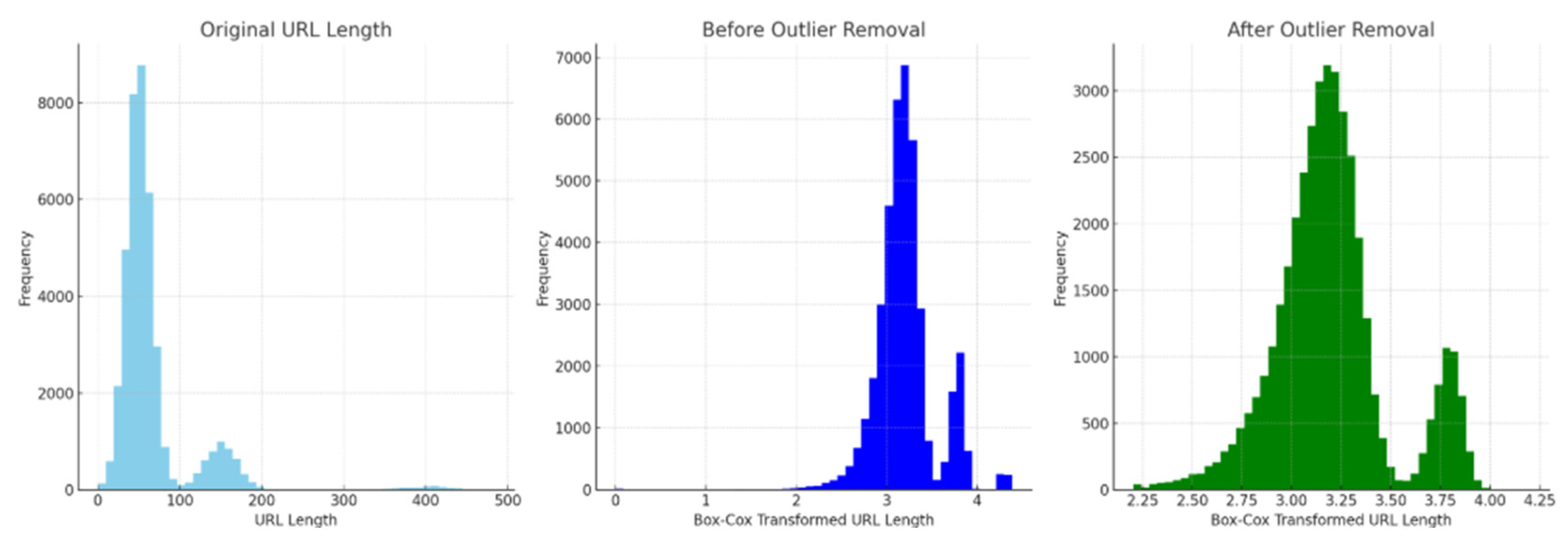
Therefore, we need to remove such outliers in our dataset. To remove such outliers, we used interquartile range techniques. The skewness level of the Box-Cox transformation technique has 0.01186 outliers and the frequency of lengthy URL occurrences is reduced to 8000. This indicates that the outliers in our custom dataset removed and achieves effective detection accuracy. Moreover, with the original URL length, the distribution is heavily right-skewed with most URLs being short and with few very long URLs. After applying the Box-Cox transformation, the data become more symmetric, but some outliers remain. Finally, after outlier removal, the distribution looks much more normal (bell-shaped), which is ideal for model training as shown in
Figure 8.
4.2.4. Performance Evaluation Metrics
For this study, evaluation metrics used to measure the performance of our models included the confusion matrix, accuracy, precision, recall, and F1-scores.
- ▪
Accuracy: Accuracy measures the overall correctness of the model by calculating the ratio of correctly predicted instances (both true positives and true negatives) to the total number of predictions.
where TP (true positive): the model correctly predicted the positive class, TN (true negative): the model correctly predicted the negative class, FP (false positive): the model incorrectly predicted the positive class, and FN (false negative): the model incorrectly predicted the negative class.
- ▪
Precision: Precision measures the accuracy of the positive predictions. It indicates how many of the predicted positive results were correct. High precision means that when the model predicts a positive, it is usually correct.
- ▪
Recall: Recall measures the ability of the model to identify all relevant instances (positives). It indicates how many actual positive cases were correctly predicted. High recall means the model captures most of the actual positives.
- ▪
F1-score: The F1-score is the harmonic mean of precision and recall. It provides a single metric that balances both precision and recall, which is especially useful when the class distribution is imbalanced. A high F1-score indicates a good balance between precision and recall.
Moreover, the Matthews correlation coefficient (MCC), which provides a comprehensive measure of classification performance considering all categories in the confusion matrix, and the area under the ROC curve (AUC-ROC), summarizing model performance across various thresholds also used. Each of these metrics plays a vital role in evaluating and interpreting the effectiveness of classification.
4.5. Experimental Results and Discussions
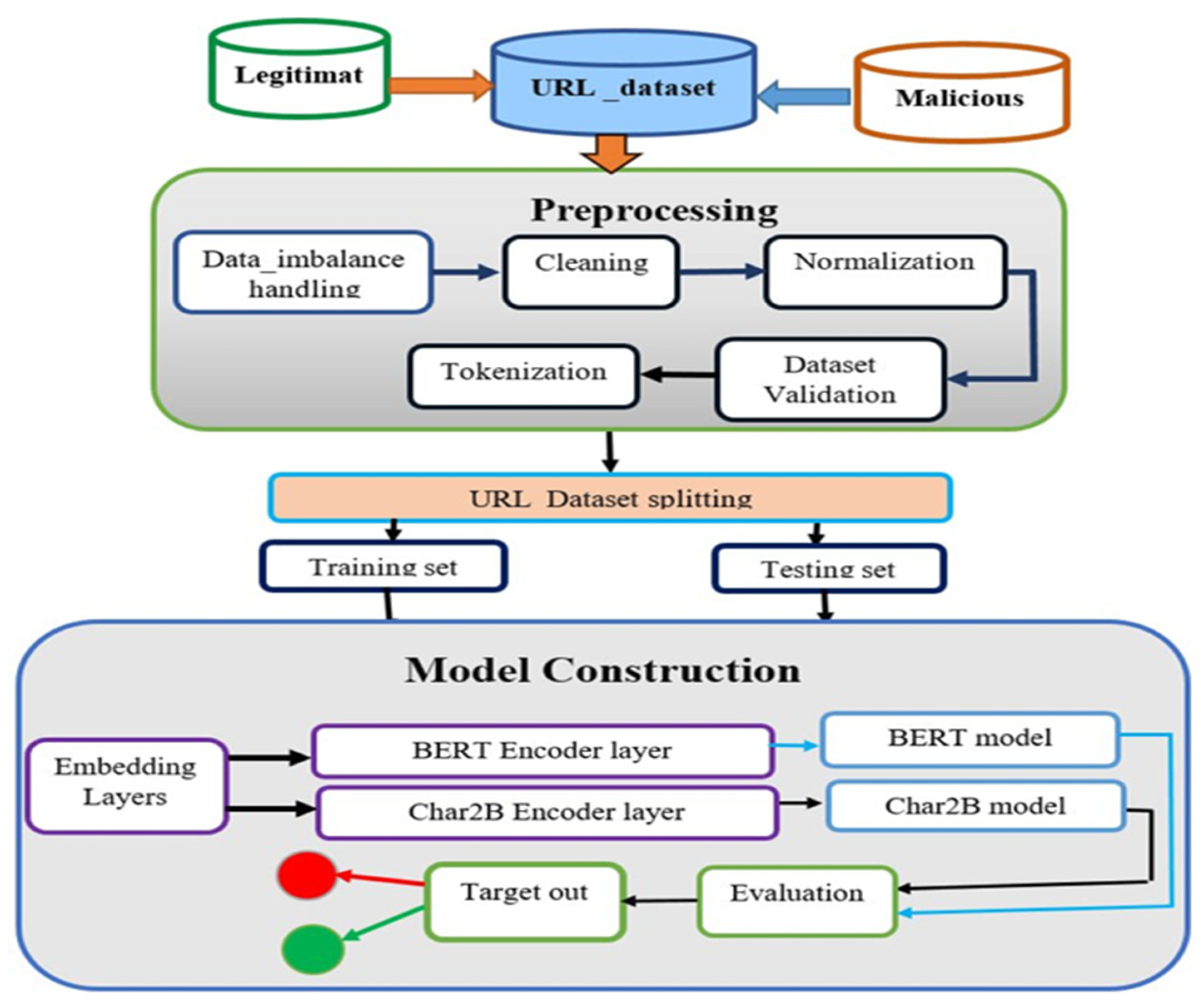
Our proposed model used the training and testing datasets to assess its performance. The processed dataset split in an 80/20% splitting ratio for training and testing sets, respectively. We used the BERT model as the base model that used to drive the Char2B model.
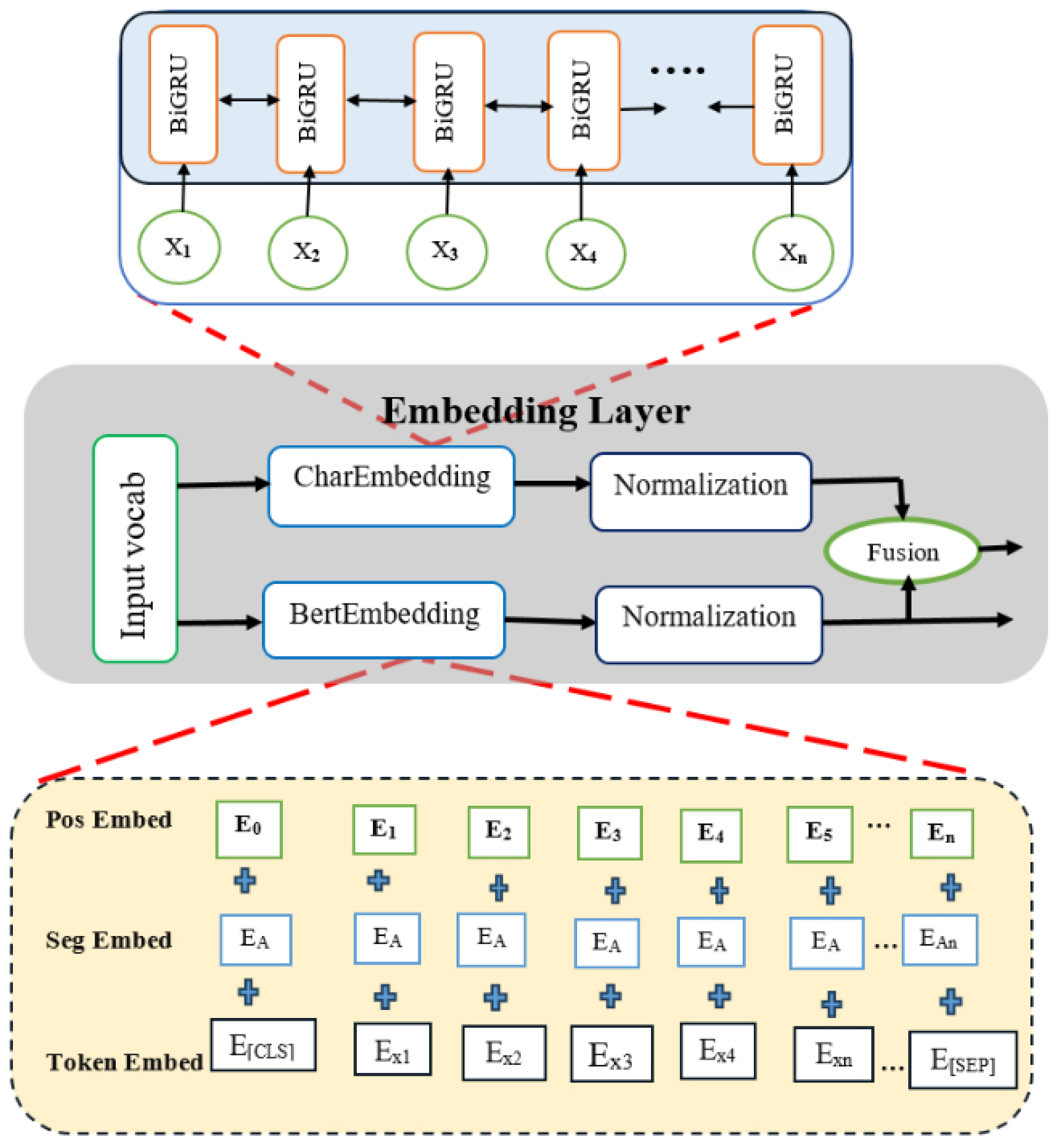
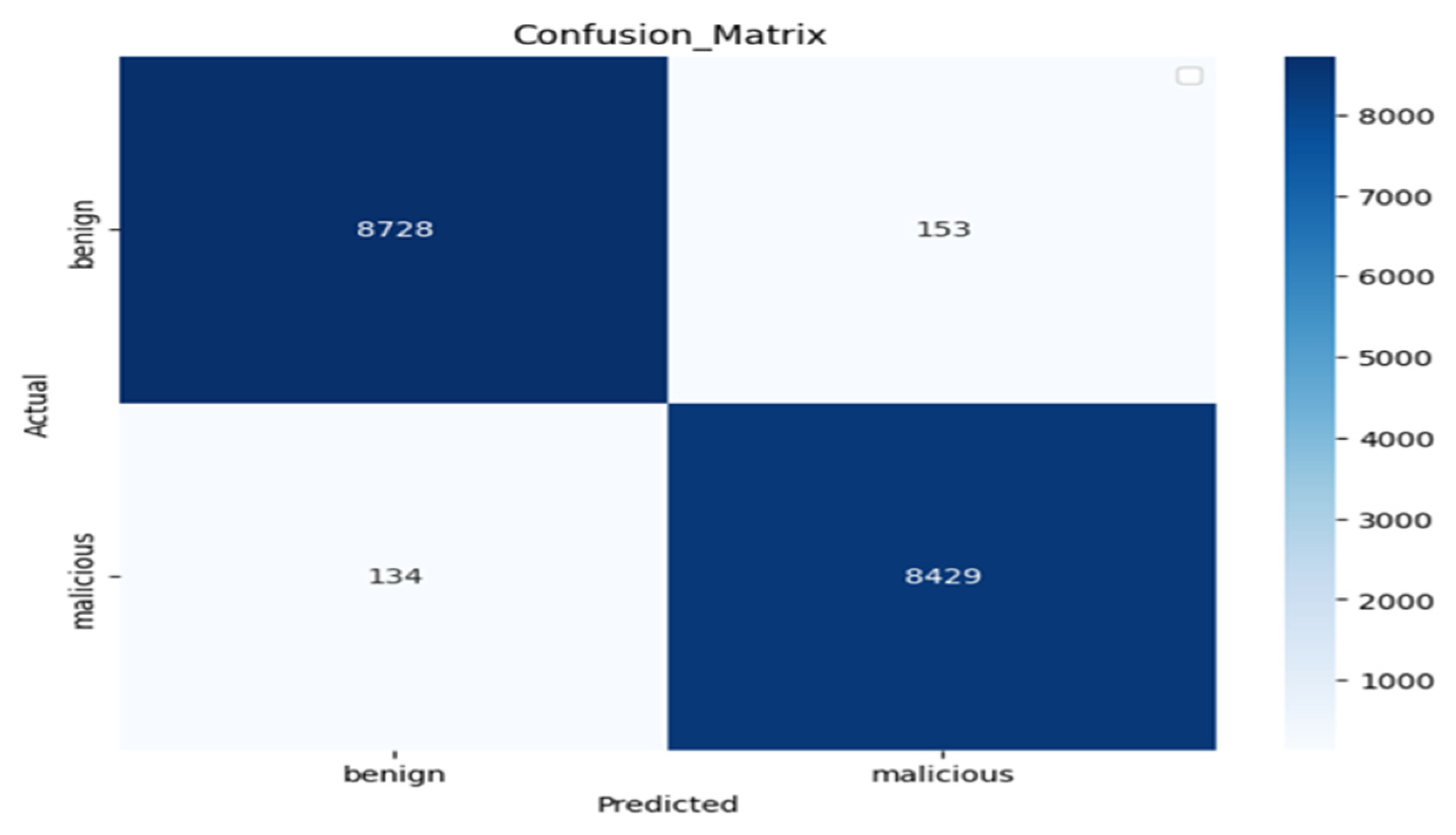
Experiment 1: We used the BERT model as the base model to construct the fusion of BERT embedding with CharBiGRU to obtain the Char2B model. The BERT model’s performance was rigorously evaluated on the test dataset using multiple metrics: a confusion matrix, classification report, and ROC curve analysis. These evaluations were conducted using consistent epoch settings across both training and testing phases, while employing different batch sizes for optimization. Therefore, as shown in
Figure 9, the number of correctly predicted negative (benign) samples out of all negative samples is 8728 with 153 samples misclassified as positive samples and the number of correctly predicted positive (malicious) samples out of the total positive samples is 8429 with 134 misclassified as negative samples.
Table 3 illustrates the training and testing performance of the base model using our dataset.
Figure 10 depicts the trade-off between the TPR and the FPR across different threshold settings, which is an essential tool for evaluating a binary classifier’s performance. In
Figure 10, the Y-axis shows the true positive rate, which is the percentage of actual positive instances that are correctly detected, while the X-axis shows the false positive rate, which is the percentage of actual negative cases that are mistakenly categorized as positive. The curve displays the classifier’s performance at various thresholds; an ideal model is represented by a TPR of one and an FPR of zero in the upper left corner of the graph.
The diagonal dashed line in the ROC graph represents a random classifier where the TPR and FPR are equal; any model along this line performs no better than chance. The model performs well in this particular curve, as seen by its placement close to the upper left corner. The classifier has a reported AUC of 0.9898, which indicates that it is quite good at differentiating between the two classes with little overlap. This high AUC value, which shows a high probability of ranking a randomly selected positive case higher than a randomly selected negative instance, supports the finding that the model is excellent at accurately recognizing positive examples while limiting false positives, with a result of 0.018. Overall, the ROC curve and its AUC offer a thorough assessment of the model’s capacity to distinguish between benign and malicious events.
Moreover,
Table 4 shows the classification report precision, recall, and F1-score: All values are 0.98 for both classes (zero and one), indicating a strong balance between correctly identifying positives and negatives. The accuracy of the overall model accuracy is 98%, meaning it correctly classified 17,444 out of 17,444 samples.
The macro and weighted averages are also both 0.98, suggesting consistent performance across classes, even with slight class imbalance (8881 vs. 8563 samples). Therefore, the classification report shows high and consistent performance and the model performs reliably and robustly, with excellent predictive ability and no sign of bias toward either class.
Figure 11 illustrates the classification report of our performance evaluation result. Out of 8881 benign test dataset samples, 98% of the dataset is correctly predicted as actually negative (benign) samples, and out of 8563 malicious test, dataset samples, 98% of samples are correctly predicted as actually positive (malicious) samples. The vertical axis displays the actual labels of the data, while the horizontal axis shows the model’s predictions, which are either benign or malicious.
The number of cases correctly predicted as benign (true negatives) is 8732, and these are located in the top left quadrant. This high number indicates that the model can accurately identify benign situations. There are 149 false positives in the upper right quadrant, which represent innocuous cases that were mistakenly labeled as malicious. Since it indicates fewer incorrect classifications of benign cases, a lower value is better in this case. The 112 false negatives that were mistakenly classed as benign are found in the bottom left quadrant. In this instance, a lower number is also preferable since it shows that harmful situations were successfully detected. The final quadrant, the bottom right one, displays 8451 true positives, or the cases that accurately classified as malicious. This high number indicates that the model can accurately detect harmful cases. We summarize the performance of the proposed model on the custom dataset using the classification report as shown in
Table 5.
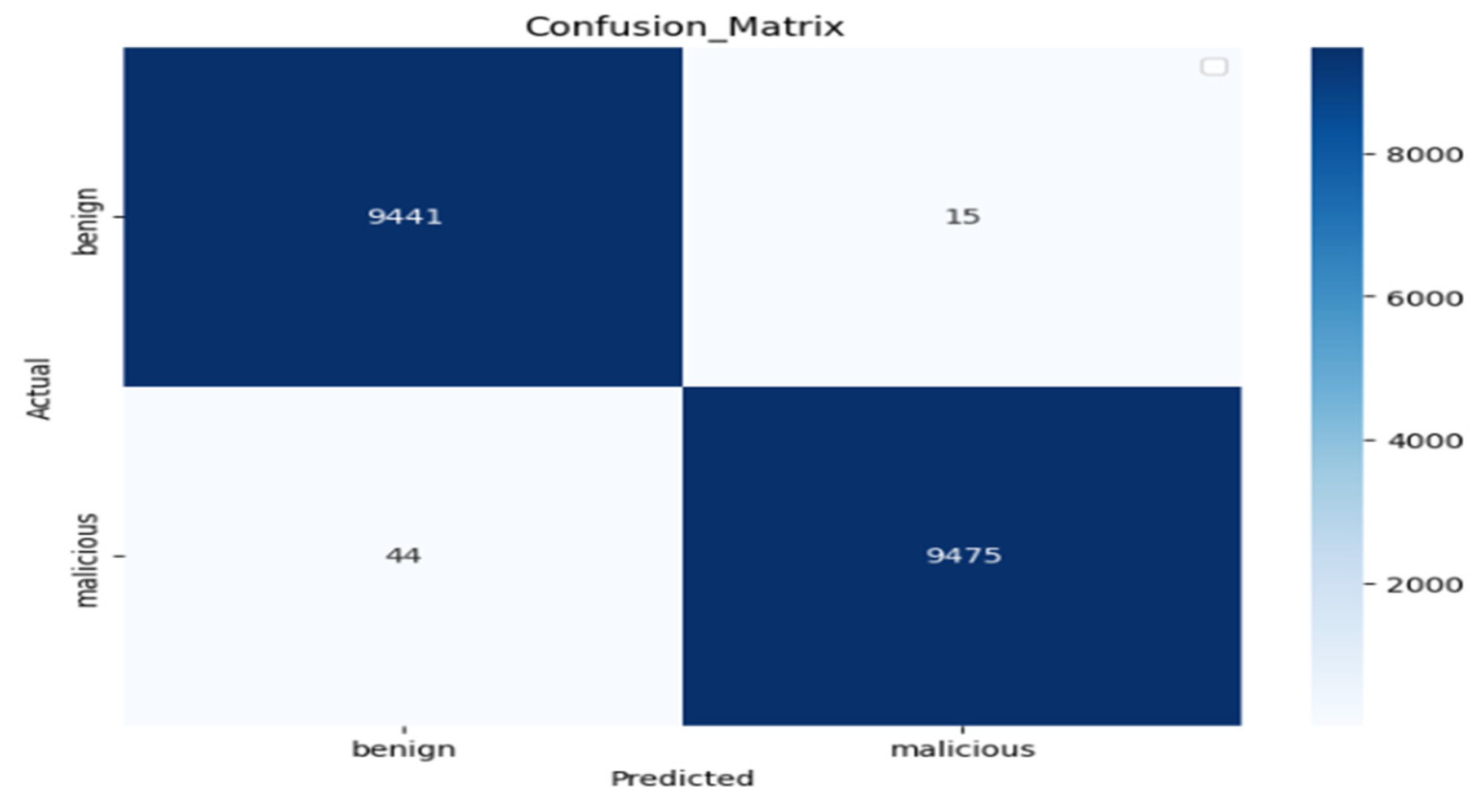
Experiment 2: We obtained our proposed Char2B model using our training dataset as well as by testing the dataset and visualizing the confusion matrix result. The confusion matrix offers a comprehensive perspective on how well a classification model performs, particularly when it comes to differentiating between benign and malicious classifications.
Next to the visualization of the performance metrics of the Char2B model using the classification report and confusion matrix, we used the ROC curve to illustrate how the model accurately distinguishes the positive (malicious) and negative (benign) samples using TPR and FPR. The ROC curve is a graphical tool used to evaluate the performance of a binary classifier by illustrating the trade-off between the TPR and the FPR at various threshold levels.
On the graph shown in
Figure 12, the x-axis represents the FPR of 0.017, measuring the proportion of actual negatives that incorrectly classified as positives, while the y-axis indicates the TPR, measuring the proportion of actual positives that were correctly identified. A diagonal dashed line represents a scenario where TPR equals FPR, indicating that a model performing no better than random guessing would lie along this line. The model’s closeness to the upper left corner of this particular ROC curve indicates that it has a high capacity for accurately classifying occurrences. Excellent discrimination between the positive and negative classes indicated by the reported AUC of 0.9965. This high AUC value indicates that there is little overlap between the classes and that the classifier is very good at differentiating between benign and malicious instances. Overall, the ROC curve and its AUC offer a thorough assessment of the model’s performance, emphasizing how well it distinguishes between the two classes while reducing incorrect classifications.
We summarized the performance of proposed model on the custom dataset using the classification report shown in
Table 6. The precision of 0.99 for class 0 and 0.98 for class 1 indicates very few false positives. The recall of 0.98 for class 0 and 0.99 for class 1 indicates very few false negatives. The F1-scores of 0.99 (class 0) and 0.98 (class 1) confirm a strong balance between precision and recall. The overall accuracy is 99%, correctly predicting 17,444 out of 17,444 samples. Finally, macro and weighted averages both are 0.99, demonstrating consistent and unbiased performance across classes. Therefore, this report reflects excellent model performance with near-perfect metrics and the model is highly effective and well generalized, showing minimal error across both classes.
4.7. Performance Comparison with the Recent Related Works
The performance of our proposed model was compared with recent state-of-the-art approaches in the domain of cybersecurity. As shown in
Table 11, we evaluated our model on two public datasets Gram-bedding and Kaggle in addition to our custom dataset. Notably, the Kaggle and Gram-bedding datasets were applied to the Char2B model without any data validation processes. The LogBERT-BiLSTM model demonstrated exceptional performance on the CSIC 2010 dataset, achieving 99.50% accuracy with flawless precision and recall rates of 100%, yielding a perfect F1-score of 100%. These results underscore the efficacy of its integrated architecture. Similarly, the CharBiLSTM-Attention model attained marginally higher performance on a custom dataset, achieving 99.55% accuracy, with 99.64% precision and 99.43% recall, resulting in an F1-score of 99.54%. The model’s attention mechanism likely enhanced its feature extraction capabilities.
In contrast, the BERT model exhibited inconsistent performance across datasets on the GitHub dataset; it achieved 96.71% accuracy, with 96.25% precision and 96.50% recall (F1-score not reported). On the ISX 2016 dataset, it reached 99.98% accuracy, though precision and recall metrics were unavailable.
Our proposed Char2B model delivered robust results on the custom dataset: 98.50% accuracy, 98.27% precision, 98.69% recall, and 98.48% F1-score. On the Kaggle dataset, it had 99.69% accuracy, 99.84% precision, 99.54% recall, and a 99.69% F1-score, demonstrating strong adaptability across diverse contexts.
Collectively, these findings indicate that Char2B competes effectively with state-of-the-art benchmarks like LogBERT-BiLSTM and CharBiLSTM-Attention, particularly in scenarios where its hybrid architecture leverages dataset-specific features.
This study aimed to develop a deep learning model capable of detecting malicious URLs that pose significant cybersecurity threats. The Char2B model developed from the baseline BERT model to evaluate whether a fused architecture could yield superior performance. Using the same dataset, our proposed model outperformed the baseline in terms of detection accuracy and FPR efficiency. For instance, the study in [
15] achieved a detection accuracy of 96.71%. Using this as a baseline, our model achieved 98.35% detection accuracy with a 0.018 FPR and a 98.98% ROC-AUC, effectively distinguishing between malicious and legitimate URLs even when tested on unseen data. Compared to the baseline, our model achieved an improvement of 0.15% on the custom dataset and 2.98% on the Kaggle dataset. Overall, these experiments suggest that fusing deep learning models, as done in Char2B, offers enhanced performance compared to relying on a single model architecture.


 ,
, 


