
Testing the Effectiveness of Voxels for Structural Analysis


Abstract
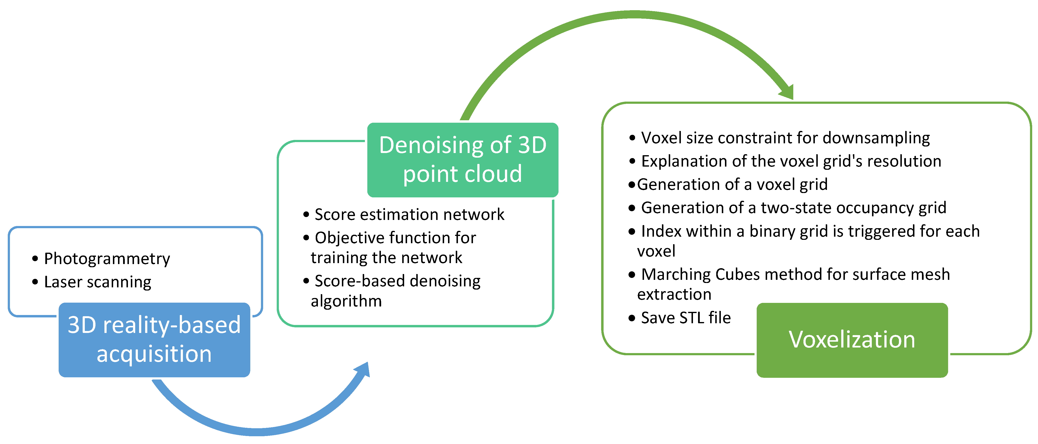
1. Introduction
1.1. Denoising
1.2. Retopology and NURBS
and a set of triangles connecting them
F = {f1,…,fF}, fi ∈ V × V × V
although it is more efficient to define the triangular mesh with the edges of the polygons
ε = {e1, …, eE}, ei ∈ V × V
- Post-processing of the mesh.
- Retopology (smoothing).
- Closing holes and checking the topology.
- NURBS.
1.3. Voxel
2. Material and Methods
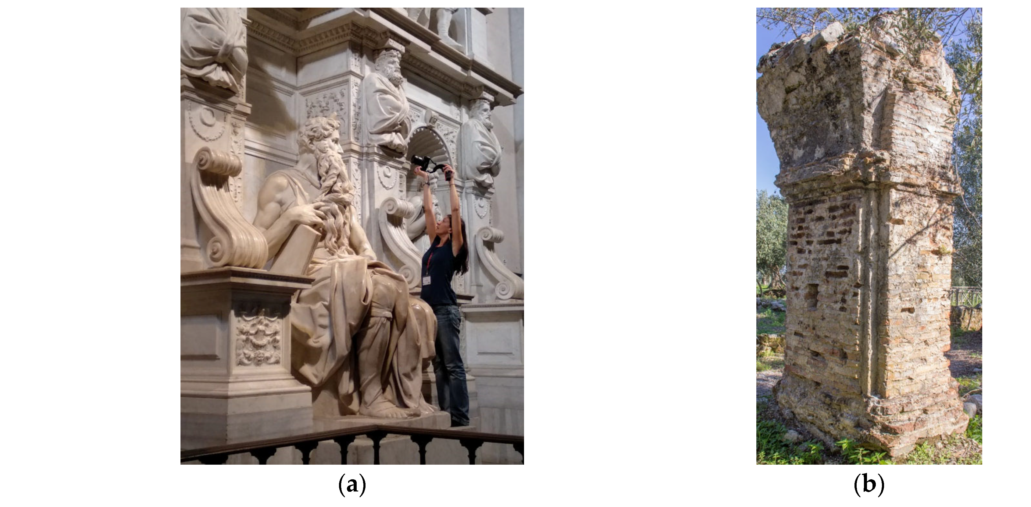
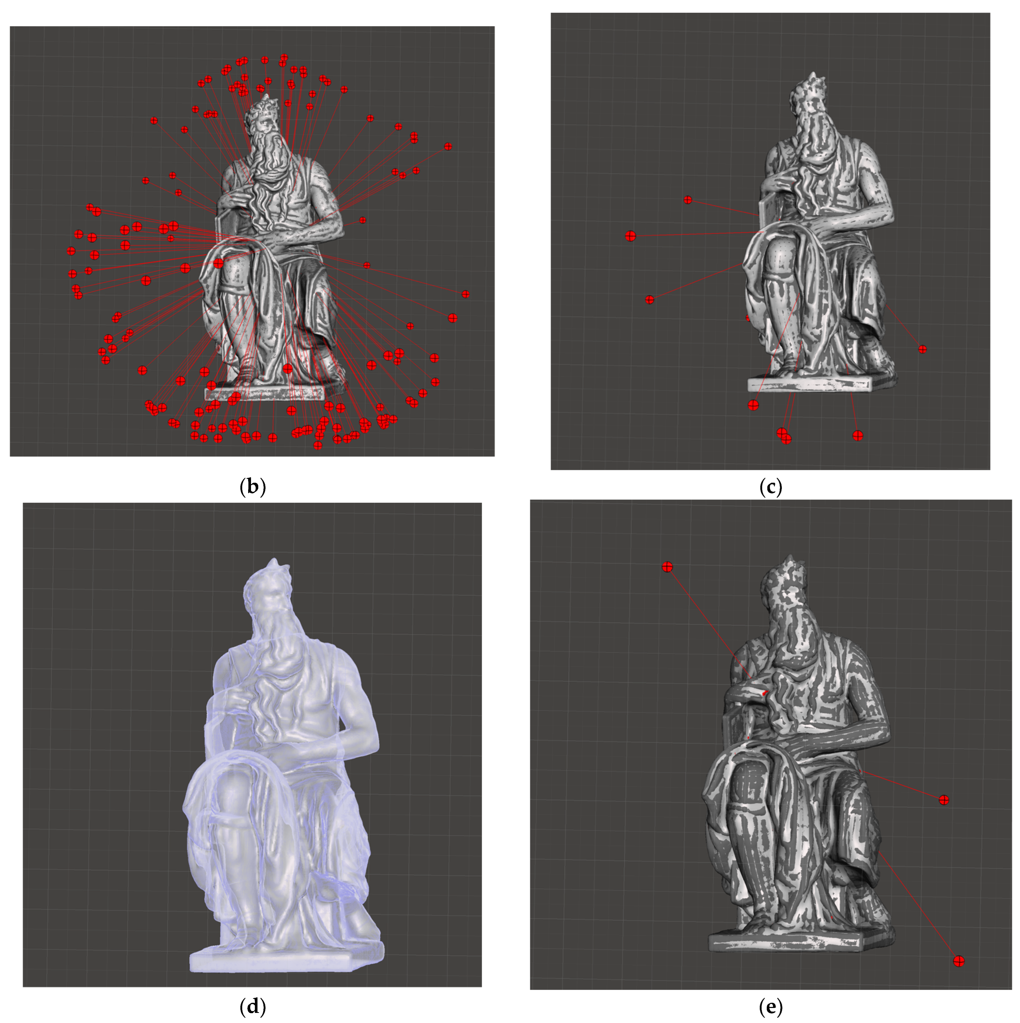
- The statue of Moses from the tomb of Pope Julius II in Rome. The problems were related to the position of the statue, so it was impossible to detect the back (Figure 1a). The problem was overcome by adding more photos of the back using illuminators to better highlight the part and using a wide lens (16 mm) that increased the field of view of the camera.
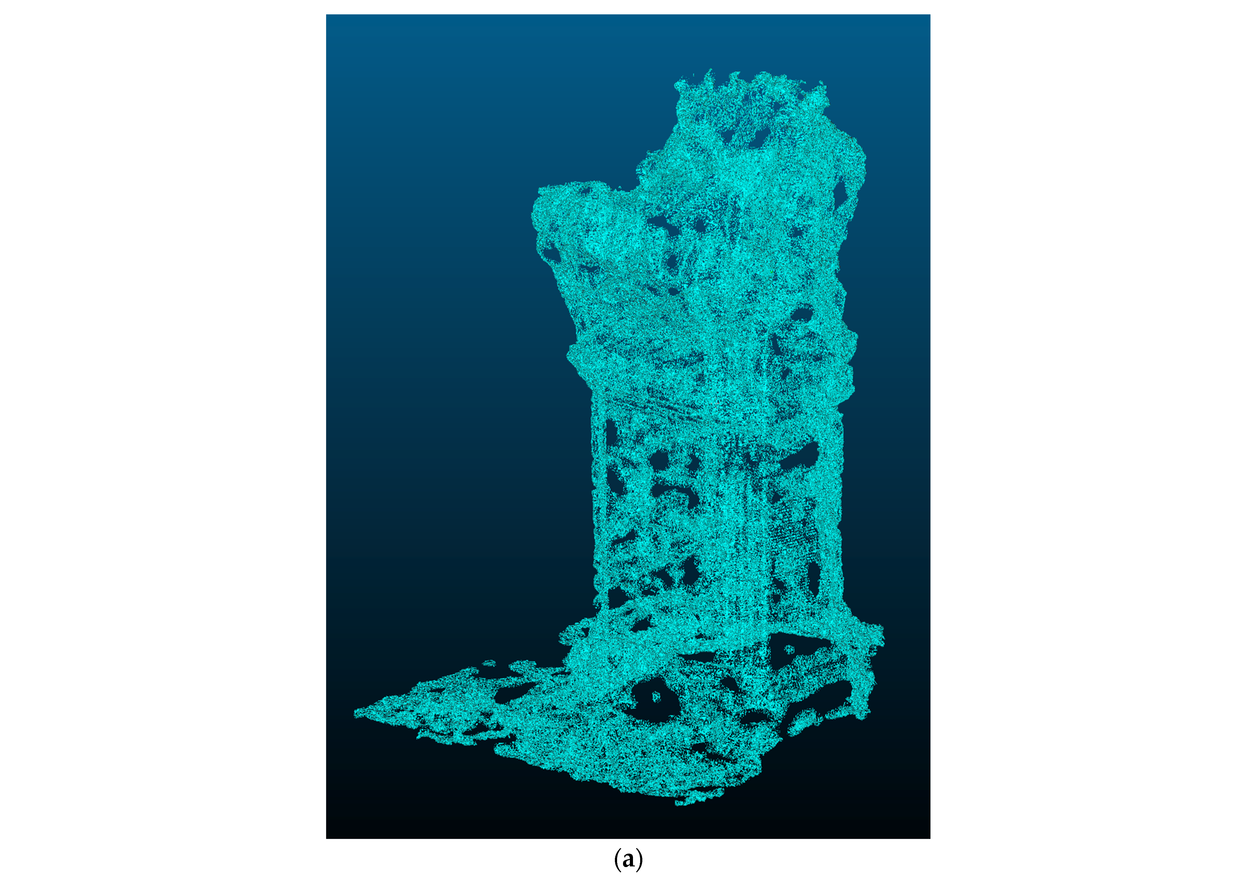
- A masonry pillar from a medieval cloister, Oppido (Italy). The problems were the presence of trees and weeds and the impossibility to detect the top of the structure (Figure 1b). This was addressed by adding images acquired with a drone. Since the cameras used were different, the point clouds were manually aligned with CloudCompare software (2.13.1).
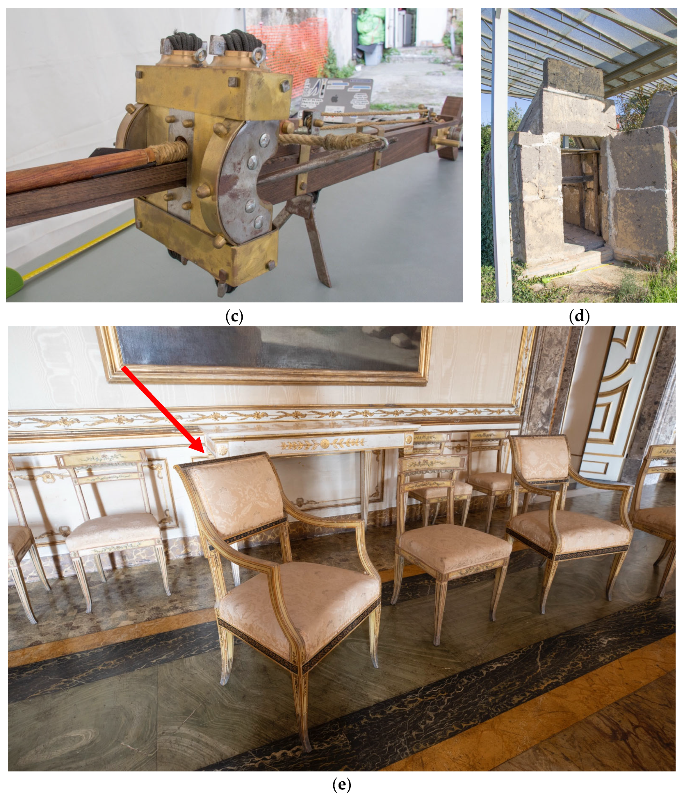
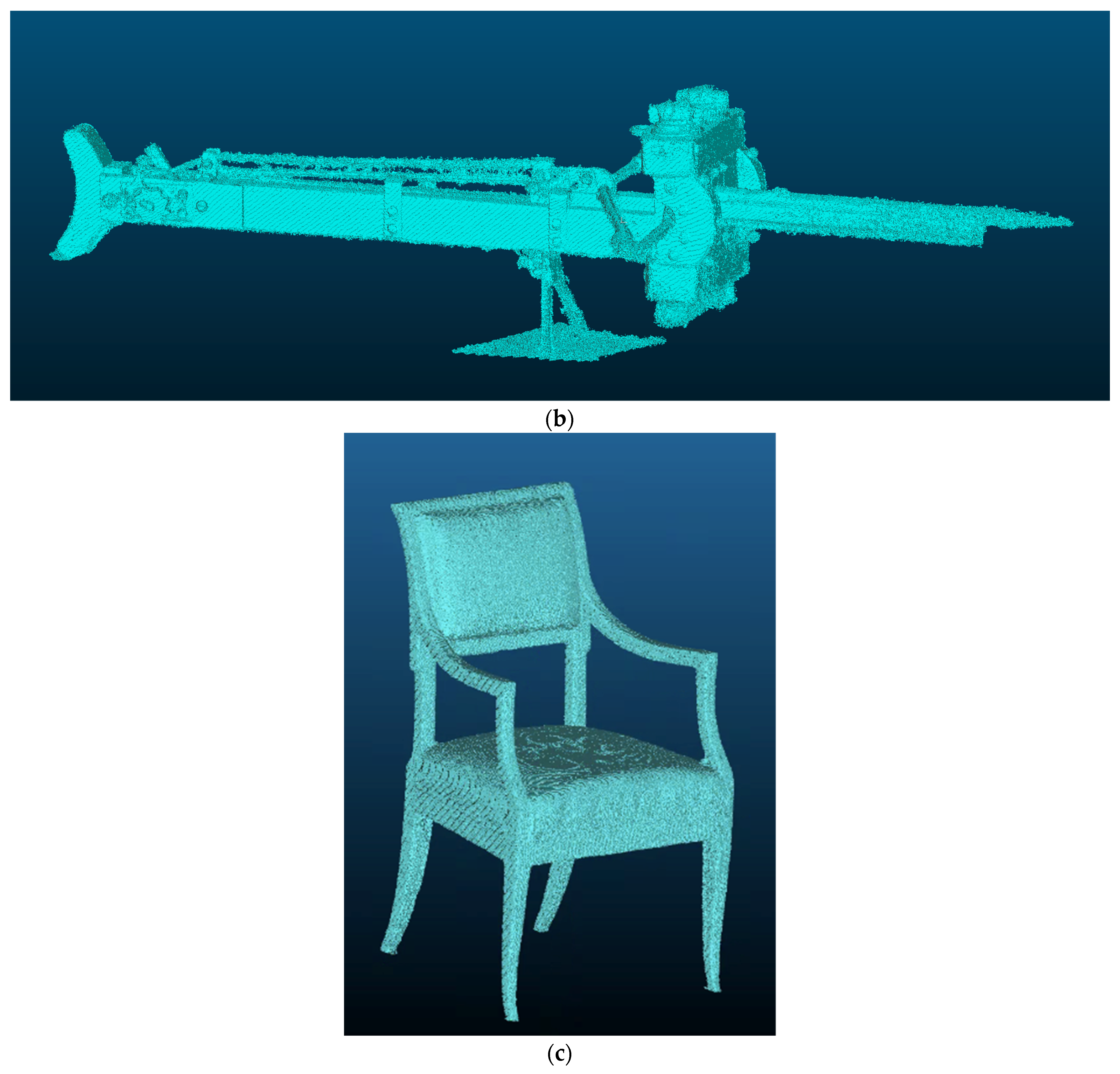
- A wooden reproduction of a Roman throwing weapon (scorpionide), with complex and detailed geometry and small and thin parts (Figure 1c). In this case, the use of a macro lens (60 mm) helped in capturing the small details. The point clouds were aligned manually with CloudCompare.
- A Samnite tomb in the archaeological park of Santa Maria Capuavetere. The structure is located on one side of the park, completely covered with ivy (Figure 1d). The point cloud was intentionally left dirty to specifically analyze the impact of the denoising algorithm on very noisy data.
3. Results
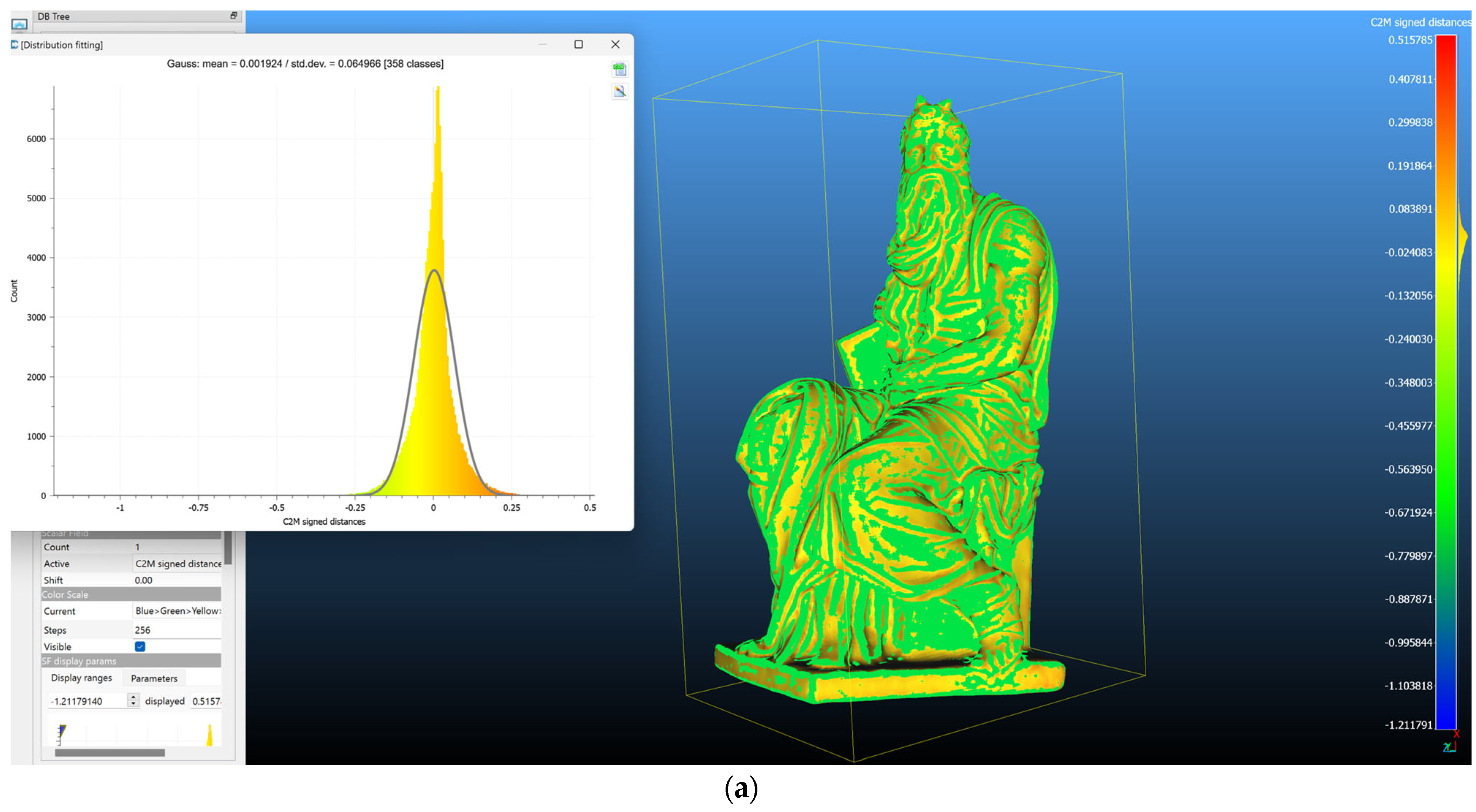
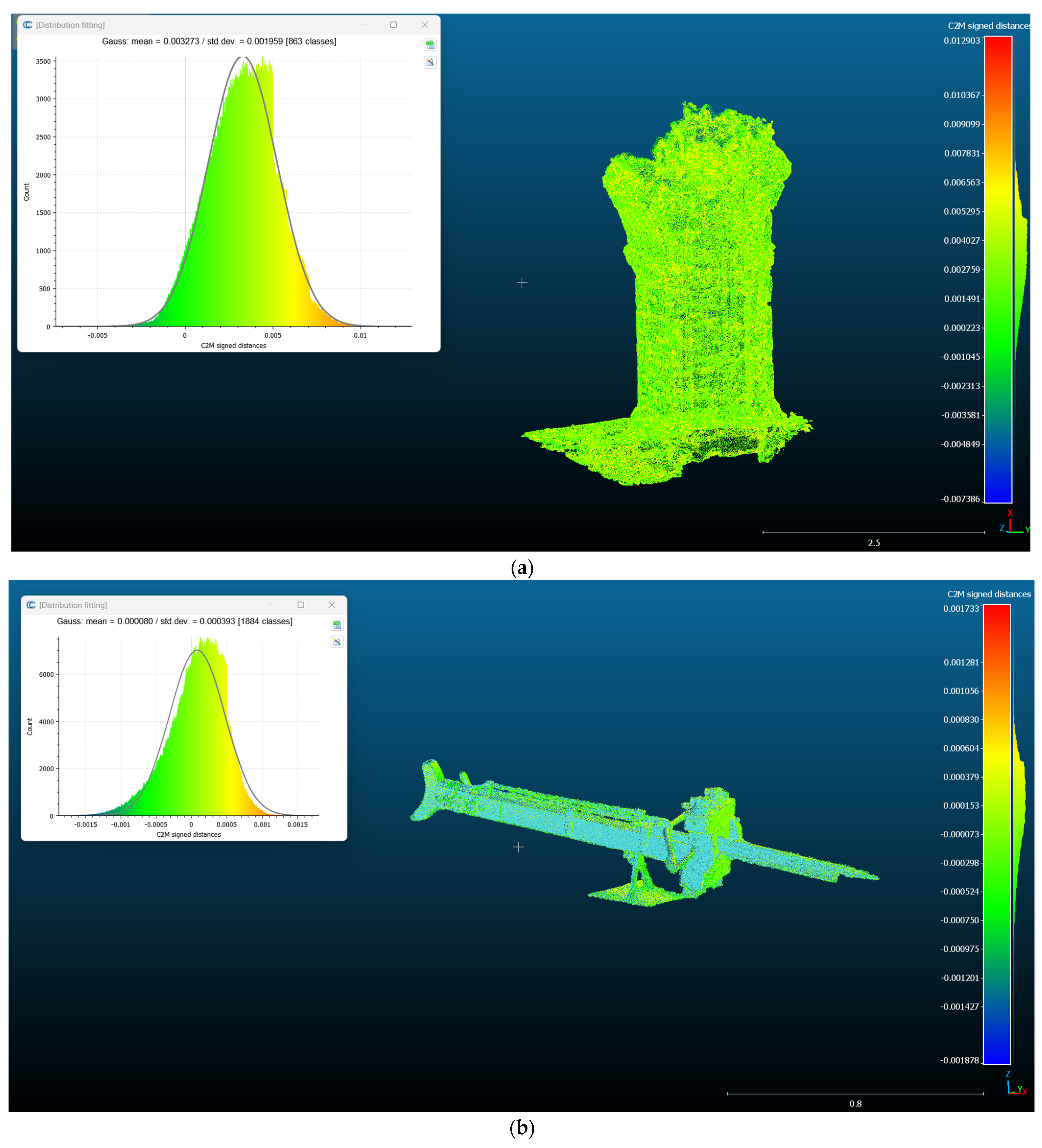
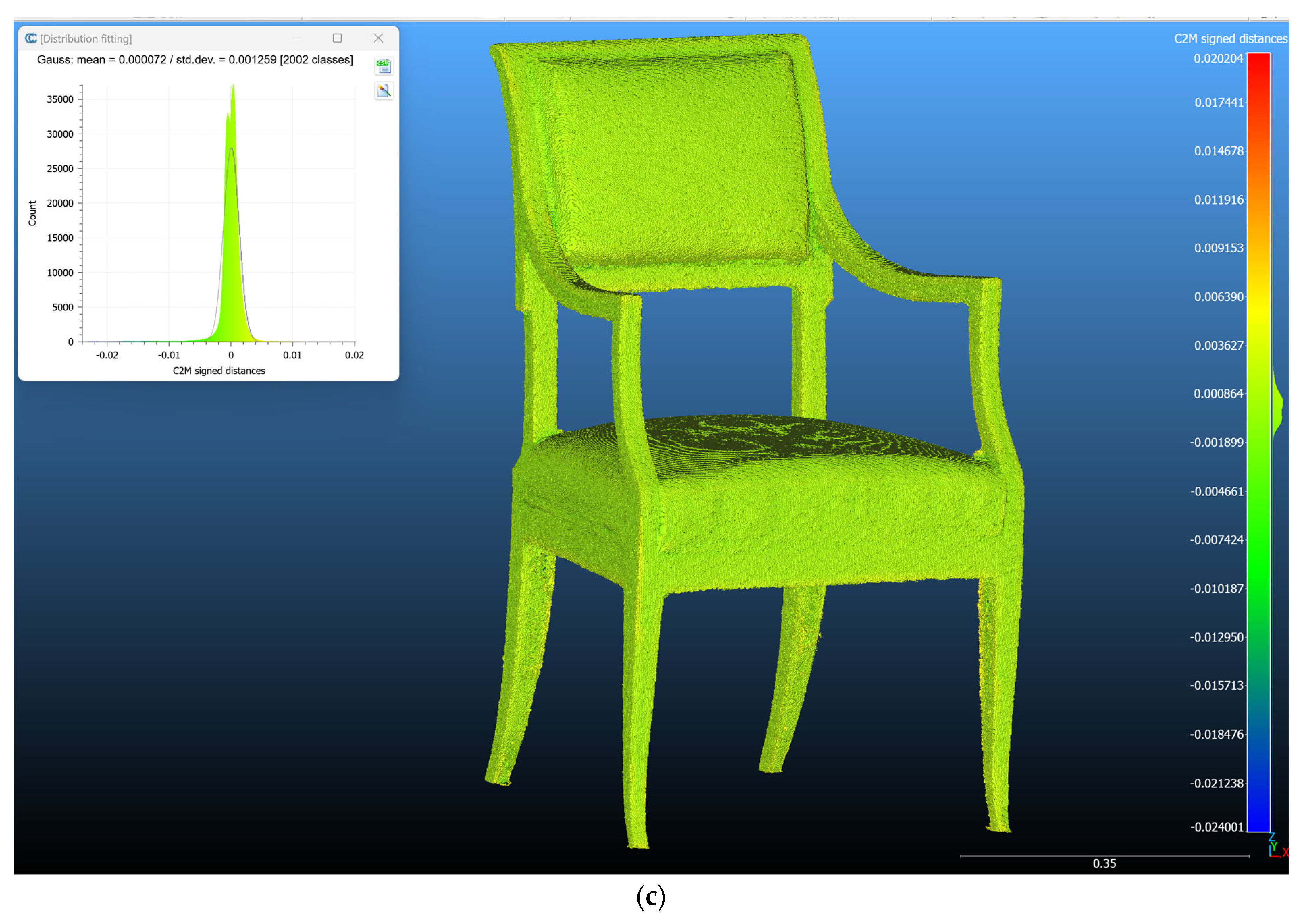
3.1. Denoising
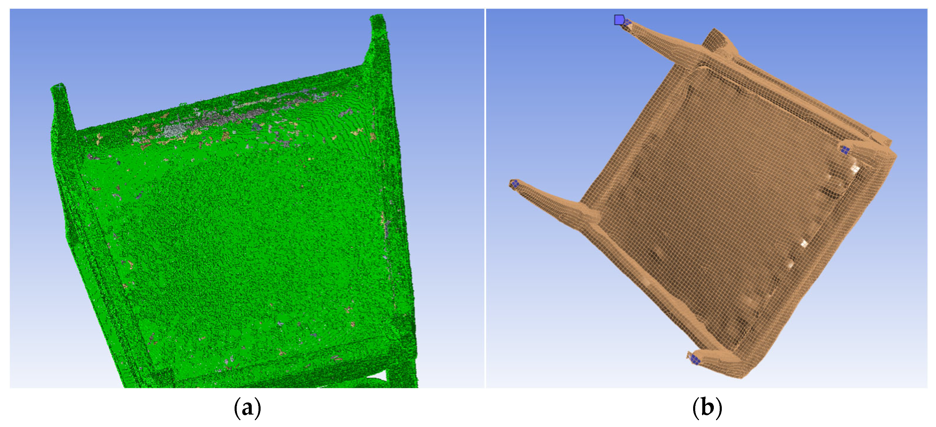
3.2. Voxelization
- Applying a voxel size constraint for downsampling.
- Explanation of the voxel grid’s resolution.
- Generation of a voxel grid.
- Generation of a two-state occupancy grid.
- For each voxel, the corresponding index within a binary grid is triggered.
- Implementation of the Marching Cubes method for surface mesh extraction.
- The STL file is subsequently stored.
- voxel_size = 0.2: Defines the resolution of the voxel grid. A smaller value results in a higher resolution but increases processing time and memory usage. The value set for this project was 0.2 because, after several tries, it was the best compromise between the best result in terms of accuracy of data obtained from the process and the exploitation of memory. The process started with the value of 0.01 and increased it considering the use of resources in terms of memory and CPU of the computer. Of course, the decision was made considering the processing effort and the accuracy of results. After several tries, 0.2 was the best choice considering the models of the object tested. It is probable that it will be possible to decrease the value in the case of smaller objects, while with bigger, more complex objects, the value will need to be increased. The voxel grid is then saved for future use.
- -
- Level = 0.5: Defines the isovalue for surface extraction. A value of 0.5 ensures that the generated mesh follows the midpoint of occupied and unoccupied voxels.
- -
- Spacing = (voxel_size, voxel_size, voxel_size): Ensures correct scaling of the output mesh relative to the original point cloud dimensions.
3.3. Test on FEA
4. Discussion
5. Conclusions
- Voxel Size Tradeoff: A finer voxel size (voxel_size < 0.2) improves surface accuracy but increases memory consumption.
- Marching Cubes Complexity: The algorithm operates on a binary grid rather than the raw point cloud, reducing noise but potentially introducing geometric artifacts.
- Denoising Optimization: Adjusting std_ratio allows for controlling the tradeoff between data retention and outlier removal.
Author Contributions
Funding
Data Availability Statement
Acknowledgments
Conflicts of Interest
References
- Höllig, K. Finite Element Methods with B-Splines; Society for Industrial and Applied Mathematic: Philadelphia, PA, USA, 2003. [Google Scholar]
- Shapiro, V.; Tsukanov, I.; Grishin, A. Geometric Issues in Computer Aided Design/Computer Aided Engineering Integration. J. Comput. Inf. Sci. Eng. 2011, 11, 21005. [Google Scholar] [CrossRef]
- Alfio, V.S.; Costantino, D.; Pepe, M.; Restuccia Garofalo, A. A Geomatics Approach in Scan to FEM Process Applied to Cultural Heritage Structure: The Case Study of the “Colossus of Barletta”. Remote Sens. 2022, 14, 664. [Google Scholar] [CrossRef]
- Brune, P.; Perucchio, R. Roman Concrete Vaulting in the Great Hall of Trajan’s Markets: A Structural Evaluation. J. Archit. Eng. 2012, 18, 332–340. [Google Scholar] [CrossRef]
- Castellazzi, G.; Altri, A.M.D.; Bitelli, G.; Selvaggi, I.; Lambertini, A. From Laser Scanning to Finite Element Analysis of Complex Buildings by Using a Semi-Automatic Procedure. Sensors 2015, 15, 18360–18380. [Google Scholar] [CrossRef]
- Erkal, A.; Ozhan, H.O. Value and vulnerability assessment of a historic tomb for conservation. Sci. World J. 2014, 2014, 357679. [Google Scholar] [CrossRef]
- Milani, G.; Casolo, S.; Naliato, A.; Tralli, A. Seismic assessment of a medieval masonry tower in northern Italy by limit, non-linear static and full dynamic analyses. Int. J. Archit. Herit. 2012, 6, 489–524. [Google Scholar] [CrossRef]
- Zvietcovich, F.; Castaneda, B.; Perucchio, R. 3D solid model updating of complex ancient monumental structures based on local geometrical meshes. Digit. Appl. Archaeol. Cult. Herit. 2014, 2, 12–27. [Google Scholar] [CrossRef]
- Kappos, A.J.; Penelis, G.G.; Drakopoulos, C.G. Evaluation of Simplified Models for Lateral Load Analysis of Unreinforced Masonry Buildings. ASCE J. Struct. Eng. 2002, 128, 890–897. [Google Scholar] [CrossRef]
- Nochebuena-Mora, E.; Mendes, N.; Lourenço, P.B.; Greco, F. Dynamic behavior of a masonry bell tower subjected to actions caused by bell swinging. Structures 2021, 34, 1798–1810. [Google Scholar] [CrossRef]
- Kyratsis, P.; Tzotzis, A.; Davim, J.P. A Comparative Study Between 2D and 3D Finite Element Methods in Machining. In 3D FEA Simulations in Machining; SpringerBriefs in Applied Sciences and Technology; Springer: Cham, Switzerland, 2023. [Google Scholar] [CrossRef]
- Pegon, P.; Pinto, A.V.; Géradin, M. Numerical modelling of stone-block monumental structures. Comput. Struct. 2001, 79, 2165–2181. [Google Scholar] [CrossRef]
- Peña, F.; Meza, M. Seismic Assessment of Bell Towers of Mexican Colonial Churches. Adv. Mater. Res. 2010, 133–134, 585–590. [Google Scholar] [CrossRef]
- Deng, J.; Shi, S.; Li, P.; Zhou, W.; Zhang, Y.; Li, H. Voxel r-cnn: Towards high performance voxel-based 3d object detection. In Proceedings of the AAAI Conference on Artificial Intelligence, Online, 11–15 October 2021; Volume 35, pp. 1201–1209. [Google Scholar]
- Bitelli, G.; Castellazzi, G.; D’Altri, A.M.; De Miranda, S.; Lambertini, A.; Selvaggi, I. Automated Voxel Model from Point Clouds for Structural Analysis of Cultural Heritage. Int. Arch. Photogramm. Remote Sens. Spatial Inf. Sci. 2016, 41, 191–197. [Google Scholar] [CrossRef]
- Doğan, S.; Güllü, H. Multiple methods for voxel modeling and finite element analysis for man-made caves in soft rock of Gaziantep. Bull. Eng. Geol Environ. 2022, 81, 23. [Google Scholar] [CrossRef]
- Karanikoloudis, G.; Lourenço, P.B.; Alejo, L.E.; Mendes, N. Lessons from Structural Analysis of a Great Gothic Cathedral: Canterbury Cathedral as a Case Study. Int. J. Archit. Herit. 2021, 15, 1765–1794. [Google Scholar] [CrossRef]
- Shapiro, V.; Tsukanov, I. Mesh free simulation of deforming domains. CAD Comput. Aided Des. 1999, 31, 459–471. [Google Scholar] [CrossRef]
- Bagnéris, M.; Cherblanc, F.; Bromblet, P.; Gattet, E.; Gügi, L.; Nony, N.; Mercurio, V.; Pamart, A. A complete methodology for the mechanical diagnosis of statue provided by innovative uses of 3D model. Application to the imperial marble statue of Alba-la-Romaine (France). J. Cult. Herit. 2017, 28, 109–116. [Google Scholar] [CrossRef]
- Freytag, M.; Shapiro, V.; Tsukanov, I. Finite element analysis in situ. Finite Elem. Anal. Des. 2011, 47, 957–972. [Google Scholar] [CrossRef]
- Oreni, D.; Brumana, R.; Cuca, B. Towards a methodology for 3D content models: The reconstruction of ancient vaults for maintenance and structural behaviour in the logic of BIM management. In Proceedings of the 18th International Conference on Virtual Systems and Multimedia, Milan, Italy, 2–5 September 2012; pp. 475–482. [Google Scholar] [CrossRef]
- Barazzetti, L.; Banfi, F.; Brumana, R.; Gusmeroli, G.; Previtali, M.; Schiantarelli, G. Cloud-to-BIM-to-FEM: Structural simulation with accurate historic BIM from laser scans. Simul. Model. Pract. Theory 2015, 57, 71–87. [Google Scholar] [CrossRef]
- Bommes, D.; Zimmer, H.; Kobbelt, L. Mixed-integer quadrangulation. ACM Trans. Graph. 2009, 28, 77:1–77:10. [Google Scholar] [CrossRef]
- Gonizzi Barsanti, S.; Guagliano, M.; Rossi, A. 3D Reality-Based Survey and Retopology for Structural Analysis of Cultural Heritage. Sensors 2022, 22, 9593. [Google Scholar] [CrossRef]
- Tomasi, C.; Manduchi, R. Bilateral filtering for gray and color images. In Proceedings of the Sixth International Conference on Computer Vision, Bombay, India, 4–7 January 1998; pp. 839–846. [Google Scholar]
- Chen, H.; Shen, J. Denoising of point cloud data for computer-aided design, engineering, and manufacturing. Eng. Comput. 2018, 34, 523–541. [Google Scholar] [CrossRef]
- Digne, J.; Franchis, C.D. The bilateral filter for point clouds. Image Process. Online 2017, 7, 278–287. [Google Scholar] [CrossRef]
- He, K.; Sun, J.; Tang, X. Guided image filtering. IEEE Trans. Pattern Anal. Mach. Intell. 2013, 35, 1397–1409. [Google Scholar] [CrossRef] [PubMed]
- Han, X.; Jin, J.S.; Wang, M.; Jiang, W. Guided 3D point cloud filtering. Multimed. Tool Appl. 2018, 77, 17397–17411. [Google Scholar] [CrossRef]
- Irfan, M.A.; Magli, E. Exploiting color for graph-based 3d point cloud denoising. J. Vis. Commun. Image Represent. 2021, 75, 103027. [Google Scholar] [CrossRef]
- Dinesh, C.; Cheung, G.; Bajíc, I.V. Point cloud denoising via feature graph Laplacian regularization. IEEE Trans. Image Process. 2020, 29, 4143–4158. [Google Scholar] [CrossRef]
- Xu, Z.; Foi, A. Anisotropic denoising of 3D point clouds by aggregation of multiple surface-adaptive estimates. IEEE Trans. Vis. Comput. Graph. 2021, 276, 2851–2868. [Google Scholar] [CrossRef]
- Rakotosaona, M.J.; La Barbera, V.; Guerrero, P.; Mitra, N.J.; Ovsjanikov, M. Pointcleannet: Learning to denoise and remove outliers from dense point clouds. Comput. Graph. Forum 2021, 39, 185–203. [Google Scholar] [CrossRef]
- Shitong, L.; Hu, W. Score-based point cloud denoising. In Proceedings of the IEEE/CVF International Conference on Computer Vision, Montreal, QC, Canada, 10–17 October 2021; pp. 4563–4572. [Google Scholar]
- Sun, J.; Ji, Y.M.; Wu, F.; Zhang, C.; Sun, Y. Semantic-aware 3D-voxel CenterNet for point cloud object detection. Comput. Electr. Eng. 2022, 98, 107677. [Google Scholar] [CrossRef]
- He, C.; Li, R.; Li, S.; Zhang, L. Voxel set transformer: A set-to-set approach to 3d object detection from point clouds. In Proceedings of the IEEE/CVF Conference on Computer Vision and Pattern Recognition, New Orleans, LA, USA, 18–24 June 2022; pp. 8417–8427. [Google Scholar]
- Mahmoud, A.; Hu, J.S.; Waslander, S.L. Dense voxel fusion for 3D object detection. In Proceedings of the IEEE/CVF Winter Conference on Applications of Computer Vision, Waikoloa, HI, USA, 3–7 January 2023; pp. 663–672. [Google Scholar]
- Shrout, O.; Ben-Shabat, Y.; Tal, A. GraVoS: Voxel Selection for 3D Point-Cloud Detection. In Proceedings of the IEEE/CVF Conference on Computer Vision and Pattern Recognition, Vancouver, BC, Canada, 18–22 June 2023; pp. 21684–21693. [Google Scholar]
- He, C.; Zeng, H.; Huang, J.; Hua, X.S.; Zhang, L. Structure Aware Single-Stage 3D Object Detection from Point Cloud. In Proceedings of the IEEE/CVF Conference on Computer Vision and Pattern Recognition (CVPR), Seattle, WA, USA, 14–19 June 2020; pp. 11870–11879. [Google Scholar]
- Lv, C.; Lin, W.; Zhao, B. Voxel Structure-Based Mesh Reconstruction From a 3D Point Cloud. IEEE Trans. Multimed. 2022, 24, 1815–1829. [Google Scholar] [CrossRef]
- Sas, A.; Ohs, N.; Tanck, E.; van Lenthe, G.H. Nonlinear voxel-based finite element model for strength assessment of healthy and metastatic proximal femurs. Bone Rep. 2020, 12, 100263. [Google Scholar] [CrossRef] [PubMed]
- Lee, T.Y.; Weng, T.L.; Lin, C.H.; Sun, Y.N. Interactive voxel surface rendering in medical applications. Comput. Med. Imaging Graph. 1999, 23, 193–200. [Google Scholar] [CrossRef] [PubMed]
- Han, G.; Li, J.; Wang, S.; Wang, L.; Zhou, Y.; Liu, Y. A comparison of voxel- and surface-based cone-beam computed tomography mandibular superimposition in adult orthodontic patients. J. Int. Med. Res. 2021, 49, 300060520982708. [Google Scholar] [CrossRef] [PubMed]
- Goto, M.; Abe, O.; Hagiwara, A.; Fujita, S.; Kamagata, K.; Hori, M.; Aoki, S.; Osada, T.; Konishi, S.; Masutani, Y.; et al. Advantages of Using Both Voxel- and Surface-based Morphometry in Cortical Morphology Analysis: A Review of Various Applications, Magnetic Resonance. Med. Sci. 2022, 21, 41–57. [Google Scholar] [CrossRef]
- Sapozhnikov, S.B.; Shchurova, E.I. Voxel and Finite Element Analysis Models for Ballistic Impact on Ceramic-polymer Composite Panels. Procedia Eng. 2017, 206, 182–187. [Google Scholar] [CrossRef]
- Cakir, F.; Kucuk, S. A case study on the restoration of a three-story historical structure based on field tests, laboratory tests and finite element analyses. Structures 2022, 44, 1356–1391. [Google Scholar] [CrossRef]
- Gonizzi Barsanti, S.; Marini, M.R.; Malatesta, S.G.; Rossi, A. A Study of Denoising Algorithm on Point Clouds: Geometrical Effectiveness in Cultural Heritage Analysis. In ICGG 2024, Proceedings of the 21st International Conference on Geometry and Graphics. ICGG 2024. Lecture Notes on Data Engineering and Communications Technologies; Takenouchi, K., Ed.; Springer: Cham, Switzerland, 2025; Volume 218. [Google Scholar] [CrossRef]
- Baert, J. Cuda Voxelizer: A Gpu-Accelerated Mesh Voxelizer. 2017. Available online: https://github.com/Forceflow/cuda_voxelizer (accessed on 6 February 2025).
- Zhou, Q.Y.; Park, J.; Koltun, V. Open3D: A modern library for 3D data processing. arXiv 2018, arXiv:1801.09847. [Google Scholar]

| Object | Camera and Lens | Parameters | Point Cloud |
|---|---|---|---|
| Masonry pillar | Canon 60D + 20/16 mm lens | ISO 250, f/10 | 2,872,140 |
| Moses | Canon 60D + 20 mm lens | ISO 250, f/8 | 1,060,629 |
| Scorpionide | Canon 60D + 18/60 mm lens | ISO 500, f/9 | 3,693,711 |
| Samnitic tomb | Canon 60D + 18 mm lens | ISO 250, f/8 | 11,238,209 |
| Chair | Canon 5D + 20 mm lens | ISO 800, f/5.6 | 2,646,151 |
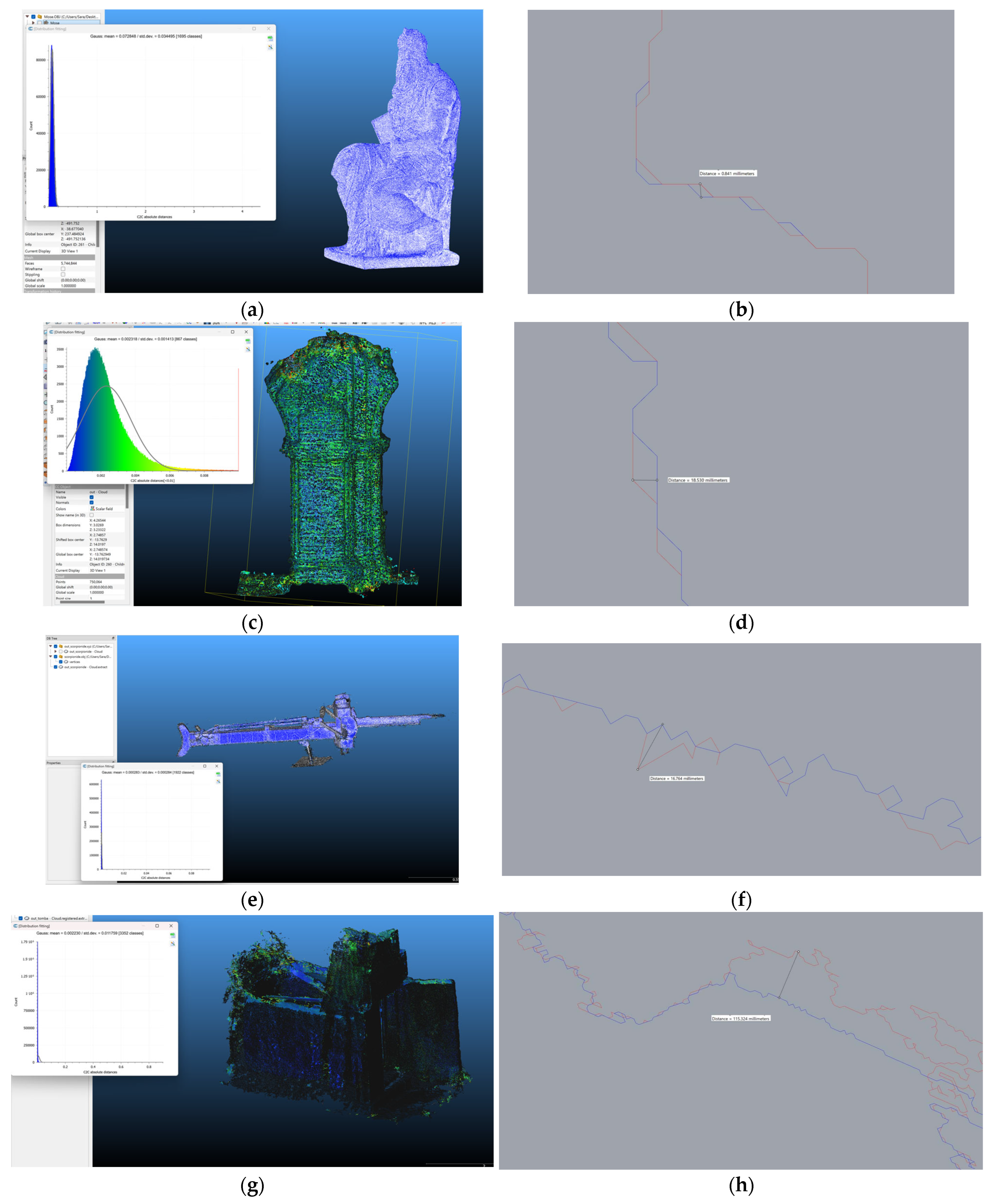
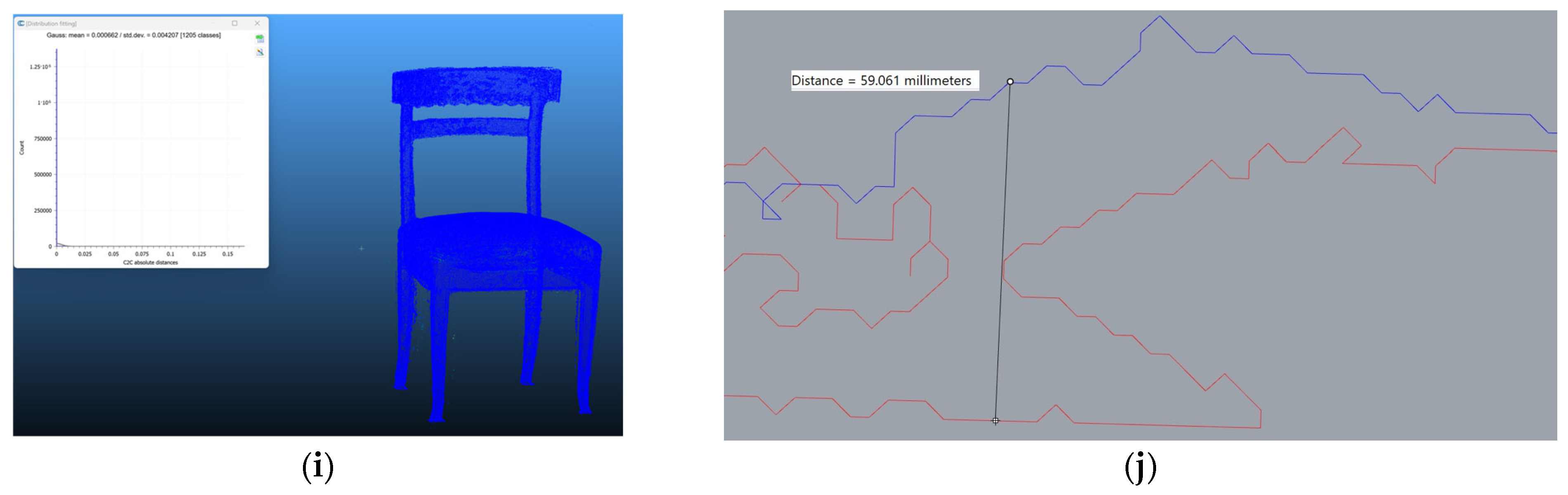
| Object | Mean (mm) | Standard Deviation (mm) | Profiles Max Distance (mm) |
|---|---|---|---|
| Moses | 0.072848 | 0.034495 | 0.841 |
| Masonry pillar | 0.002318 | 0.001413 | 18,530 |
| Scorpionide | 0.0002883 | 0.000284 | 316,764 |
| Samnitic tomb | 0.002230 | 0.011759 | 115,324 |
| Chair | 0.0007 | 0.004 | 59 |
| Object | Mean (m) | Standard Deviation (m) |
|---|---|---|
| Masonry pillar | 0.003 | 0.002 |
| Scorpionide | 0.00008 | 0.000393 |
| Chair | 0.0014 | 0.0009 |
Disclaimer/Publisher’s Note: The statements, opinions and data contained in all publications are solely those of the individual author(s) and contributor(s) and not of MDPI and/or the editor(s). MDPI and/or the editor(s) disclaim responsibility for any injury to people or property resulting from any ideas, methods, instructions or products referred to in the content. |
© 2025 by the authors. Licensee MDPI, Basel, Switzerland. This article is an open access article distributed under the terms and conditions of the Creative Commons Attribution (CC BY) license (https://creativecommons.org/licenses/by/4.0/).
Share and Cite
Gonizzi Barsanti, S.; Nappi, E. Testing the Effectiveness of Voxels for Structural Analysis. Algorithms 2025, 18, 349. https://doi.org/10.3390/a18060349
Gonizzi Barsanti S, Nappi E. Testing the Effectiveness of Voxels for Structural Analysis. Algorithms. 2025; 18(6):349. https://doi.org/10.3390/a18060349
Chicago/Turabian StyleGonizzi Barsanti, Sara, and Ernesto Nappi. 2025. "Testing the Effectiveness of Voxels for Structural Analysis" Algorithms 18, no. 6: 349. https://doi.org/10.3390/a18060349
APA StyleGonizzi Barsanti, S., & Nappi, E. (2025). Testing the Effectiveness of Voxels for Structural Analysis. Algorithms, 18(6), 349. https://doi.org/10.3390/a18060349