Abstract
In this work, the construction of adaptive one-dimensional computational grids is considered using a numerical method and physics-informed neural networks (PINNs). The grid adaptation process is described by the diffusion equation, which allows for the redistribution of nodes based on a control function. The numerical method employs an iterative scheme that adjusts the node positions according to the solution gradients, ensuring local refinement in key regions. In the PINN approach, the governing equation is incorporated into the loss function, enabling the neural network model to generate the grid based on physical constraints. To evaluate the performance of both methods, tests are conducted with different control function parameters, and the influence of diffusion coefficients on grid adaptation is analyzed. The results show that the numerical method leads to sharper variations in node spacing, while PINNs produce a smoother grid distribution. A comparative analysis of the deviations between the methods is performed. The obtained data allow for assessing the characteristics of grid adaptation in both approaches and for identifying possible directions for their further application in numerical modeling tasks.
1. Introduction
In many areas of mathematical physics, solving complex physical problems often requires numerical approaches, especially when analytical solutions are unavailable or impractical. One of the foundational components of these numerical methods is the construction of computational grids, which play a key role in both the accuracy and efficiency of simulations. Fine grids offer more accurate results, particularly in regions where the solution changes rapidly, while coarser grids help reduce the computational cost in smoother regions.
Adaptive mesh generation techniques aim to strike a balance between these two needs by adjusting the grid dynamically, refining it in critical areas and coarsening it where possible. This adaptability is especially valuable in simulations involving sharp gradients or localized phenomena.
Recent advancements in machine learning, particularly physics-informed neural networks (PINNs), have opened new possibilities for solving partial differential equations while incorporating physical laws directly into the learning process. This study explores the application of PINNs to adaptive grid generation for the one-dimensional diffusion equation. By leveraging the equidistribution principle within a neural network framework, we aim to generate grids that respond automatically to the behavior of the solution, providing an efficient and accurate numerical tool for further simulations.
The study in [1] is dedicated to the numerical modeling of two-dimensional gas flows using adaptive curvilinear grids. The method of equidistribution is applied, allowing for automatic node refinement in regions with high flow gradients, thereby improving calculation accuracy. The studies in [2,3] explore the theoretical foundations of grid generation, including solutions to partial differential equations and variational methods. The studies in [4,5] propose methods for generating two- and three-dimensional grids by solving elliptic equations and optimizing node distribution. High-performance computing studies in [6] demonstrate the potential of parallel computations for accelerated grid generation.
Computational grids are generally classified as either structured or unstructured. Structured grids utilize algebraic, differential, and variational methods to maintain a uniform node distribution while adapting to the problem’s physical characteristics [7]. In unstructured grids, Delaunay triangulation and Voronoi diagrams are employed to achieve efficient and uniform grid generation for complex geometries [8,9]. Elliptic methods and adaptive strategies also play a crucial role in optimizing node density based on computational conditions [7]. Both approaches are actively evolving and widely used in numerical modeling. However, the adaptive modification of grid density remains a challenging task that requires careful consideration of the system’s physical properties.
One of the most powerful approaches to generating such meshes is to formulate the problem as a boundary value problem for a system of differential equations. In particular, inverse diffusion equations, Poisson equations, and especially Beltrami equations have found wide application in this regard [10]. The use of differential equations in mesh generation differs from their classical application. In typical problems of mathematical physics, differential equations describe physical processes (such as heat conduction, diffusion, and wave propagation), whereas in mesh generation, they are used to define the transformation of coordinates from the computational domain to the physical domain. In this context, the variables in the equations are interpreted as geometric parameters of the mesh (e.g., coordinate functions), and their derivatives represent mesh distortion measures or node density. Thus, the application of differential equations in adaptive mesh generation is not merely a technical tool but rather a fundamental mathematical framework for creating unified and controllable models of computational meshes adapted to the physics of the problem and the geometry of the domain. These approaches have proven effective in computational fluid dynamics and finite element analysis, ensuring high mesh quality and alignment with the physical features of the solution [11].
One-dimensional computational grids are widely used in various applied problems, such as hydrodynamics, continuum mechanics, and electrodynamics. This study examines the construction of a one-dimensional adaptive computational grid based on the diffusion equation. This equation regulates grid density by refining the node distribution in regions with steep solution gradients. Existing research has employed different approaches to construct adaptive computational grids using the diffusion equation. The study in [12] presented an unstructured grid generation method using differential techniques, achieving adaptation via the inverse Beltrami equation. The authors proposed using Delaunay triangulation for final grid construction, ensuring the smoothness of the geometric characteristics of grid cells. In [13], the application of Beltrami and diffusion equations for numerical grid generation was explored, taking into account the physical properties of the modeled medium. Later, [14] introduced an algorithm for generating three-dimensional adaptive grids, utilizing inverse Beltrami equations to construct grids in multiscale domains. The study in [15] examined variational and elliptic grid generation methods that optimize node distribution while considering boundary conditions. Additionally, [16] proposed a fragmented algorithm for adaptive grids, implementing automated computational fragment management in the LuNA system, which efficiently distributes computing resources for complex simulations.
In recent years, PINNs have gained significant attention for solving differential equations, including the diffusion equation. Numerous studies have demonstrated the successful application of PINNs to problems involving heat conduction, mass transport, and other processes described by diffusion-type models [17,18,19]. By embedding physical laws directly into the loss function, such models can produce stable and interpretable solutions, even when data are limited or noisy. The studies in [20,21,22,23] explore various extensions of PINNs, including hybrid models, variational approaches (VPINN), and Bayesian methods (B-PINN), which improve solution accuracy and stability. In these methods, the network is trained with physical constraints, reducing dependence on large training datasets. The study in [24] investigates the application of PINNs to solve equidistribution equations for constructing two-dimensional adaptive computational grids. PINNs allows for approximate equation solutions without explicit discretization by integrating physical laws into the loss function. Recent research has utilized neural networks for automated grid generation and adaptation. The study in [25] applies graph neural networks (GNNs) to predict and optimize grids in hydrodynamics and mechanics. In [26], a method for generating finite element meshes based on self-organizing Kohonen maps is proposed. The study in [27] explores the use of GNNs for adaptive grid generation in numerical methods. These studies confirm the potential of machine learning in optimizing grid construction, reducing computational costs, and enhancing simulation accuracy.
However, the use of PINNs specifically for adaptive mesh generation through node distribution control based on the diffusion equation has received little attention in the literature. Existing works on PINNs typically focus on the accuracy of the solution but do not examine the structure of the computational mesh implicitly formed during training. At the same time, the distribution of training points—the implicit “mesh” shaped by loss minimization—has a significant impact on the final model quality. While there are studies that apply PINNs to problems involving geometry and spatial adaptation [25,27,28,29], a comprehensive approach that directly employs the diffusion equation as a mechanism for mesh adaptation within the PINN framework is currently lacking.
Additionally, the method of solving the diffusion equation and the inverted Beltrami equation provides a continuous mapping from the sample domain to the physical domain, which can be leveraged to enhance the accuracy of PINNs. The key motivation of this research is to integrate, in future, the curvilinear mapping obtained from these equations into the PINN framework itself rather than using it solely for classical numerical grids. By doing so, the PINN method can better adapt to regions with steep gradients, where its accuracy is often compromised due to an insufficient resolution or inadequate sampling. This hybrid approach combines the flexibility of neural networks with the rigorous control of mesh adaptation, offering a promising solution to improve PINN performance in challenging scenarios. The results of this work may pave the way for more robust and accurate physics-informed machine learning models in computational physics and engineering simulations.
An additional objective addressed in this work is the hard enforcement of boundary conditions during adaptive grid generation. In most existing approaches, boundary conditions are implemented through penalty terms in the loss function, which requires the manual tuning of weighting coefficients and may not guarantee strict enforcement at the boundaries. In the proposed approach, boundary values are explicitly fixed through the network architecture by embedding a smooth mask that suppresses the neural network output at the edges of the interval [30]. This allows for physically consistent results without introducing extra parameters into the loss function.
The proposed method differs from previously published work by combining adaptive grid generation based on the diffusion equation with hard boundary condition enforcement directly within the PINN architecture.
2. Materials and Methods
This section presents methods for constructing one-dimensional adaptive computational grids using the diffusion equation. Two approaches are considered: the traditional numerical solution via the finite difference method and a neural network-based approach utilizing PINNs.
2.1. Algorithm for Constructing a One-Dimensional Structured Computational Grid
One-dimensional structured computational grids play a crucial role in numerical modeling, providing high solution accuracy through a uniform node distribution within the study domain. This section describes an approach to constructing such grids using a one-dimensional diffusion equation, which accounts for the physically significant properties of the medium. To enhance the efficiency and versatility of the method, an algorithm based on PINNs is developed, where the diffusion equation is directly embedded in the loss function. This allows for physical constraints to be taken into account without explicit parametric approximation. The one-dimensional diffusion equation used in the development of structured computational grids is described as follows:
where is an independent parametric variable, is the target function describing the node distribution, and is the weighting function that controls the grid density. The function plays a key role, analogous to the diffusion coefficient in multidimensional problems. This equation is based on balancing the gradients of the function , which describes the spatial arrangement of nodes, while considering the weighting function , which defines the local grid density. From a physical perspective, this equation represents a deformation of the coordinate space: regions requiring a higher resolution receive a denser grid, while areas of lesser significance are allocated fewer nodes. If takes on larger values in certain regions, the grid is refined in these areas, increasing the accuracy of numerical computations. Conversely, when is lower, the grid becomes coarser, reducing computational costs in less critical regions. From a physical perspective, this balance can be seen as a distribution of local forces: determines the local resistance or “weight” of a region, while the derivative describes the variation in the target function in this space. This equilibrium results in a grid that optimally accounts for the specific features of the problem.
Boundary conditions play a crucial role in constructing adaptive computational grids, as they define the shape and distribution of nodes within the modeling domain. In the standard formulation, the boundary conditions are defined as follows:
where and denote the initial and final coordinates of the computational domain. These conditions ensure a strict fixation of the grid’s boundary points to the specified limits.
Boundary conditions also influence the distribution of nodes within the computational domain. For example, in problems with sharp solution gradients, boundary conditions can be combined with the weighting function to refine the grid near regions with high parameter variability. The numerical solution is implemented by discretizing the space and applying approaches such as the finite difference method. The result of the solution is the function , which defines the adaptive distribution of computational grid nodes optimized for the given problem. This approach ensures high accuracy in critical regions while minimizing computational costs. In the general case of three-dimensional space, the parametric coordinate is represented as , and the corresponding mapping of the computational grid is defined by the function .
This equation forms the foundation of the developed method, which is integrated with neural networks to efficiently solve one-dimensional grid generation problems. This approach combines solving the diffusion equation with automatic differentiation to create a grid with adaptive node density.
2.2. Implementation Using PINNs
2.2.1. Fundamental Principles of PINNs
The PINN is a method that combines the capabilities of neural network modeling with physical laws. Unlike traditional neural networks, which rely solely on data, the PINN incorporates differential equations as additional constraints, allowing the model to account for physically justified dependencies during training. This approach is particularly useful in numerical modeling problems, where obtaining accurate and stable solutions requires integrating the knowledge of fundamental natural laws.
One of the key advantages of the PINN is its ability to approximate solutions to differential equations without explicit domain discretization. This mitigates common numerical method challenges, including accuracy dependence on grid resolution and the need for explicit iterative schemes. Specifically, to construct an adaptive one-dimensional computational grid, the diffusion equation is incorporated into the neural network’s loss function, ensuring a physically meaningful result.
However, despite these advantages, the PINN method may exhibit a lower solution accuracy than traditional numerical methods. This is because minimizing the loss function does not always guarantee strict adherence to the original differential equation, especially in the presence of complex control functions with sharp variations. Additionally, the choice of hyperparameters, such as network architecture, learning rate, and loss function parameters, significantly impacts the final solution accuracy. In some cases, the PINN method may smooth out local grid features, leading to discrepancies compared to numerical methods.
In the presented implementation, a PINN is applied to solve the one-dimensional diffusion equation, where the network is trained to ensure that its output values satisfy both the equation and the given boundary conditions. This is achieved by using automatic differentiation in PyTorch https://pytorch.org/ (accessed on 11 April 2025), which allows for the direct computation of the derivatives of the network’s output values and the minimization of the physics-informed loss function. This approach provides high flexibility in constructing computational grids and enables the generation of optimal node distributions.
One possible way to improve the accuracy of the PINN method is to introduce an additional mapping of the reference domain, which allows for better control over the node distribution in the adaptive grid. Applying parametric transformations to input data or adjusting the weighting function can provide a more precise correspondence between the analytical solution and the predictions of the neural network model.
To evaluate the effectiveness of different strategies for enforcing boundary conditions in PINNs, two neural network architectures are implemented in this study. The first architecture imposes Dirichlet boundary conditions via a penalty term in the loss function, while the second applies a hard constraint using a smooth mask function embedded into the output layer.
2.2.2. Neural Network Architecture
The developed neural network model for constructing a one-dimensional computational grid based on the diffusion equation is a multilayer fully connected network implemented in PyTorch. The main goal of this architecture is to approximate the function , which is the function governing adaptive grid node distribution, while ensuring compliance with the diffusion equation. The architecture of the neural network used in this study is shown in Figure 1. The model consists of an input layer, several hidden layers with sigmoid activation functions, and an output layer that approximates the target function. The diffusion equation is incorporated into the loss function, enabling the model to learn in a physically consistent manner.
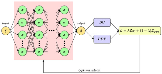
Figure 1.
Architecture of the PINN used to generate the adaptive grid.
The total loss function is defined as
where is a weighting coefficient that controls the contribution of the boundary conditions and the differential equation to the total error. This formulation ensures the normalization of the total loss and provides an intuitive interpretation of the relative importance of each component.
Neural Network Structure
The network architecture consists of 10 hidden layers, each containing 5 neurons. The input to the network is the one-dimensional coordinate x, while the output is the value s(x), which defines the position of the computational grid nodes. The network layers are structured as follows:
- -
- Input layer: Accepts the one-dimensional value x and passes it to the first hidden layer.
- -
- Ten hidden layers: Each layer contains five neurons, fully connected. A sigmoid activation function is used to introduce nonlinearity into the model.
- -
- Output layer: Transforms the output values of the last hidden layer into a one-dimensional value s(x) without applying an activation function, as this is a regression task.
Weight Initialization Methods and Input Data Normalization
The network weights are initialized randomly following a standard distribution. The input data x are normalized before being processed by the network, which improves convergence during training.
Optimal Hyperparameters
The model’s hyperparameters include the following:
- Number of hidden layers: 10;
- Activation function: Sigmoid;
- Optimizer: Adam;
- Learning rate: 0.01;
- Number of training iterations: 40,000.
The selected parameters ensure a balance between prediction accuracy and computational efficiency.
Implementation of the Diffusion Equation as Part of the Loss Function
In this implementation, the diffusion equation is incorporated into the loss function, allowing the neural network model to satisfy physical constraints without explicitly constructing the grid. This is achieved by automatically differentiating the network’s output data and minimizing deviations from the equation.
The loss function consists of two components:
1. Constraint on the diffusion equation. Using automatic differentiation in PyTorch, the first derivative is computed and weighted by the function . Then, the second derivative is calculated, where , which should be equal to zero. This condition is incorporated into the loss function as follows:
Here, represents the loss function associated with the diffusion equation. The value of quantifies the deviation of the neural network’s output from the equation. A lower indicates a better approximation of the solution.
2. Boundary Conditions. To ensure a physically meaningful result, an additional error term is introduced at the edges of the computational domain:
Here, enforces the boundary conditions by minimizing the difference between the predicted and true values at the domain boundaries.
In this implementation, the chosen hyperparameters ensure a balance between solution quality and computational efficiency. One of the key hyperparameters is the learning rate. The model uses the adaptive Adam optimizer with an initial learning rate of . This optimization method dynamically adjusts the gradient step size based on parameter update magnitudes. A learning rate that is too high can cause instability, while a rate that is too low may result in prolonged training with little improvement in the results.
Input values x are randomly sampled within , defining the parametric space for computational grid construction. Boundary conditions are fixed at the domain edges to ensure proper grid formation and solution stability. All data are processed in tensor format for efficient computation, with CUDA parallelism accelerating GPU-based calculations [31].
2.2.3. PINN Architecture with Hard Enforcement of Boundary Conditions
To construct a one-dimensional adaptive computational grid, a PINN architecture is implemented in which the diffusion equation is directly embedded into the loss function. A key feature of the model is the hard enforcement of Dirichlet boundary conditions—without introducing additional penalty terms in the loss. The boundary conditions are enforced by embedding a special smooth mask into the architecture, which vanishes at the boundaries and and remains positive inside the interval. The model output is defined as follows:
where is the neural network output responsible for the internal adaptation of the grid, and suppresses this output at the domain boundaries. The mask is defined as the product of two approximate distance functions to the ends of the interval:
where each function is constructed as follows:
with being the normalized distance to the boundary, and
defining a truncated influence region centered in the middle of the interval. This mask construction is smooth and differentiable, which is crucial for stable training with automatic differentiation in PINNs.
This approach guarantees the strict satisfaction of boundary conditions during prediction, avoiding the need for the manual tuning of boundary weights in the loss function and ensuring the physical consistency of the results.
A schematic of the implemented architecture is shown in Figure 2, illustrating the computational flow from input , through the modified output block with the mask , to the evaluation of the loss based on the diffusion equation.
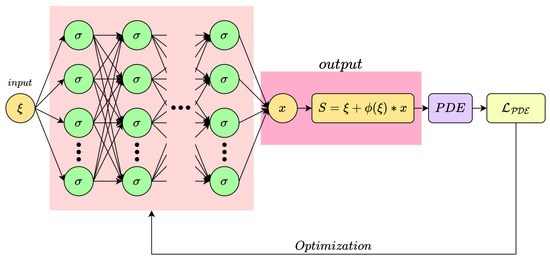
Figure 2.
PINN architecture with embedded mask for hard enforcement of boundary conditions in adaptive grid generation.
Since the boundary conditions in this architecture are enforced directly at the output level, the final loss function contains only the component associated with satisfying the differential equation, that is, without any coefficient.
The proposed approach of the hard enforcement of boundary conditions using a built-in mask function is especially promising for extension to two-dimensional adaptive mesh generation. In 2D settings, local refinement often leads to distortion near boundaries, causing grid lines along the domain edges to bend or deviate from their intended positions. This is particularly problematic when boundary shapes must remain fixed or aligned with the physical geometry. The architecture presented in this work, which guarantees the strict satisfaction of boundary conditions at the neural network output level, offers a robust solution to this issue. By construction, the boundary nodes remain fixed, regardless of internal adaptation, making this method well suited for accurate and geometry-preserving adaptive meshing in higher-dimensional problems.
2.3. Implementation of the Sequential Method
2.3.1. Numerical Solution of the Diffusion Equation
For the numerical solution of the one-dimensional diffusion equation, the finite difference method is used. The core idea of this approach is to discretize the differential equation and replace derivatives with finite difference approximations. In this implementation, the equation is solved using an iterative relaxation method, which enables the determination of the grid node distribution that corresponds to the given weighting function.
Discretization of the Diffusion Equation
The one-dimensional diffusion equation is expressed in the form of Equation (1). For the numerical solution, the domain is divided into uniformly spaced nodes with step size , leading to a system of finite difference equations. The derivatives are approximated using central differences:
which results in a finite difference scheme for determining . This scheme accounts for the influence of the weighting function , which defines the grid density in different regions of the computational domain.
2.3.2. Iterative Solution Algorithm
An iterative relaxation method is used for the numerical solution of the diffusion equation, sequentially adjusting the grid node values until a stable distribution is achieved. The method is based on updating the values at each node while considering information from neighboring nodes. At each step, new values are computed using the following approximation:
where J represents the coefficients that depend on the weighting function and the spatial step.
A crucial aspect of the method is its stability. Iterations incorporate value smoothing to prevent abrupt changes in grid density and to facilitate gradual node adaptation.
To monitor convergence, a stopping criterion is used: the process continues until the difference between the node values at two consecutive steps becomes smaller than a specified accuracy threshold .
The numerical method for solving the equation is based on the iterative adjustment of computational grid nodes until a stable distribution is achieved. During each iteration, node positions are recalculated considering the weighting function, which defines the grid density in different regions.
Boundary conditions are fixed at the beginning of the computation and remain unchanged throughout the entire process. The algorithm’s convergence is monitored by evaluating the changes in node values, allowing for automatic termination once the desired accuracy is achieved. After completing the iterations, the final node distribution is saved for further analysis and visualization.
3. Results
This section presents numerical experiments conducted to solve the one-dimensional diffusion equation given in the form (1). The control function plays a key role in forming the adaptive grid, allowing for node clustering in selected regions of the computational domain. In the numerical tests, the following form of the control function is used:
where are the coordinates of the points near which an increased node density is required, is the coefficient controlling the intensity of local refinement, and is a smoothing parameter that prevents singularities and abrupt changes in density. During testing, the positions of , as well as the values of and , are varied to examine how different characteristics of the control function influence grid generation using both the numerical method and the PINN approach.
To evaluate the characteristics of one-dimensional computational grid generation using both the numerical method and the PINN method, tests are conducted with various control function parameters. During the experiments, the parameters (which determines the intensity of node clustering) and (which controls the degree of smoothing of the control function) are varied. A fixed control point at x = 0.5 is used, and the grid coordinates are distributed within the interval .
The tests utilize the following parameter combinations: and . This allows for an evaluation of the impact of each parameter on grid adaptation and differences in node distribution.
The test results are presented as graphs analyzing the node distributions for both methods, spacing between points, coordinate differences between nodes, cumulative curves, and convergence rate of the loss function. Below is a detailed analysis of each of these aspects. Figure 3 illustrates the impact of parameter on the node distribution in both the numerical method and the PINN method.
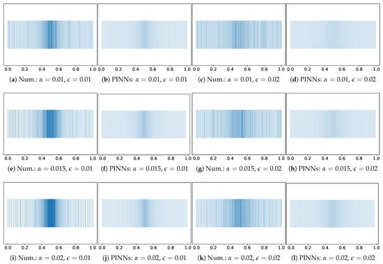
Figure 3.
Node distribution graphs.
As increases, local node clustering intensifies, which is more pronounced in the numerical method, where the node density near the control points increases significantly. In the PINN method, increasing also affects grid adaptation; however, clustering occurs more smoothly, without abrupt jumps in the distribution. Parameter determines the degree of smoothing of the control function, and its increase leads to a more uniform node distribution in both methods. In the numerical method, this results in reduced sharp step variations, while in the PINNs, smoothing causes less pronounced node density adaptation around the control point, making the distribution more uniform.
Figure 4 presents graphs of the step size between neighboring nodes, illustrating the differences in grid adaptation between the numerical method and PINNs.
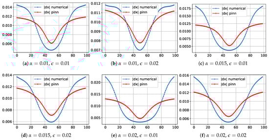
Figure 4.
Graphs of step size variation between neighboring nodes.
In the numerical method, more pronounced step size minima are observed near the control points, corresponding to the given function . In the PINN method, step size variations occur more smoothly, without abrupt minima, which may be related to the optimization characteristics of the model. The shapes of the graphs in both methods maintain the general trend of step size reduction in the regions of node clustering and increase near the boundaries of the computational domain. However, in the numerical method, the step changes are more abrupt, whereas in the PINNs, the transitions are smoother. Figure 5 shows a graph of the absolute difference between the node coordinates in the two methods.
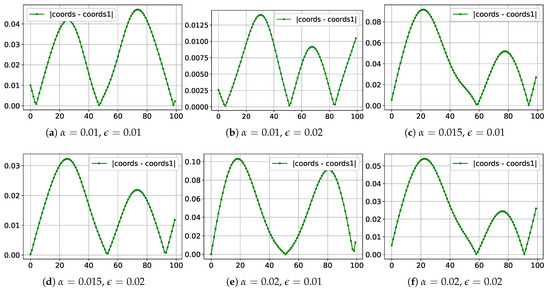
Figure 5.
Graphs of the difference between node coordinates.
It can be seen that the largest discrepancies occur near the region of node clustering. For small values of , the difference between the methods remains insignificant. However, as increases, the numerical method exhibits a sharper change in grid density, leading to greater coordinate deviations. Parameter also affects the nature of the differences between the methods: as increases, the discrepancies decrease since both methods exhibit less pronounced grid clustering. The maximum deviation, depending on the parameters of the control function, ranges from 0.01 to 0.1, and most tests show a difference within 0.03–0.05.
Figure 6 presents a cumulative node curve, which illustrates the overall trend of the node distribution across the computational domain and shows how uniformly the node coordinate changes with respect to its index.
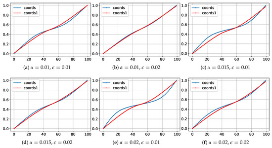
Figure 6.
Graphs of cumulative node curves.
In the numerical method, small segments with changes in the curve’s slope are observed near the control points, corresponding to local grid refinement. In the PINN method, the cumulative curve changes more uniformly, without sharp bends, indicating a smoother variation in the node density. The overall shape of the curves in both methods remains similar; however, the numerical method exhibits more pronounced slope changes, while in the PINNs, the transitions are less abrupt.
Figure 7 presents loss function graphs, illustrating the convergence dynamics of the PINN method depending on the control function parameters.
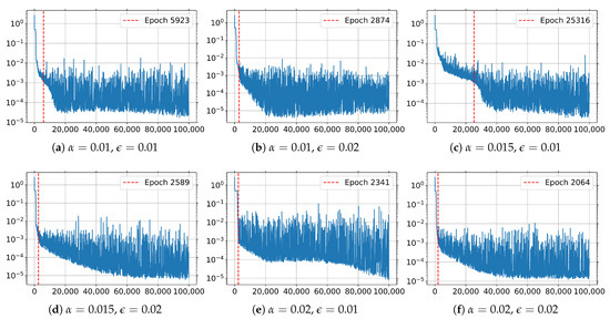
Figure 7.
Loss function graphs for the PINN method.
In all tests, the loss function decreases to 0.001; however, the convergence rate varies. Increasing and decreasing require more iterations to reach the specified error threshold, which may be due to the model’s more complex adaptation to sharp changes in the control function. In tests with and , the error threshold is reached more quickly, whereas for and , significantly more epochs are required for convergence. The results indicate that smoothing the control function positively affects the convergence speed of the PINN method, while increasing the intensity of grid clustering leads to longer training times.
To analyze the adaptation of the computational grid to multiple control points, tests are conducted with parameters and . In this case, node clustering is considered near two control points, and , within the interval . This allows for an evaluation of how effectively the numerical method and the PINN method reproduce the specified grid density distribution when multiple regions with high node concentrations are present. As part of the testing, graphs are generated for the node distribution, step sizes between neighboring points, coordinate differences between the methods, cumulative curves, and convergence rate of the loss function in the PINN method.
Below is a detailed analysis of the obtained results, including a comparison of both methods based on key indicators such as the degree of grid clustering, uniformity of the node distribution, deviations between the numerical method and PINNs, and specific features of neural network model convergence. Figure 8 shows the node distribution in the numerical method and the PINN method for control points and .
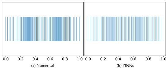
Figure 8.
Graphs of node distribution at coordinates 0.3 and 0.7.
In both methods, an increase in the node density is observed near the control points. In the numerical method, node clustering occurs more abruptly, whereas the PINN method exhibits a smoother grid density distribution without sharp jumps. Despite differences in approach, both methods successfully adapt the grid to the given parameters. However, the numerical method produces more pronounced gradients in the node distribution, while the PINN method shows some smoothing in high-density regions. Figure 9 presents the key grid characteristics, including the step size variation between neighboring nodes, coordinate differences between the methods, cumulative node curves, and loss function.
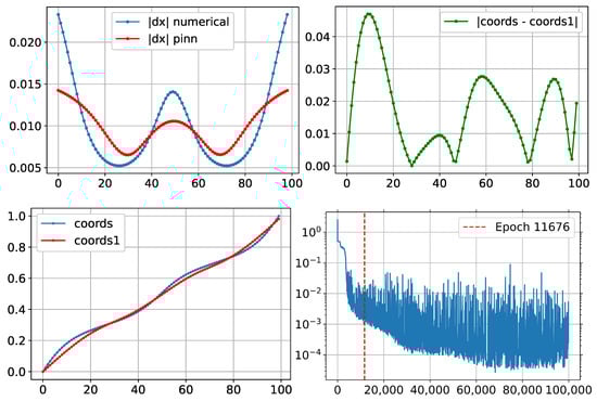
Figure 9.
Graphs of node distribution at coordinates 0.3 and 0.7.
Both approaches demonstrate the expected node clustering near the control points; however, the numerical method results in more abrupt density variations, whereas the PINN method produces a smoother distribution. The coordinate differences between the nodes indicate that the maximum discrepancy is 0.05, which can be attributed to the smoothing effect of neural network optimization. The cumulative curves of both methods confirm the overall grid adaptation trend, though the numerical method exhibits more pronounced slope changes. The loss function graph shows that the PINN method requires more iterations to achieve an accurate result but ultimately reaches high precision, minimizing the error to 0.000026. These results highlight the characteristics of each method and provide insights into their applicability for adaptive computational grid generation.
Hard Enforcement of Boundary Conditions: Comparison of Approaches
To evaluate the effectiveness of the hard enforcement of boundary conditions using the mask , a series of numerical experiments are conducted comparing two approaches: implementing boundary conditions through an additional penalty term in the loss function and enforcing them explicitly by modifying the neural network output. Figure 10a shows the node distribution obtained using the mask , while Figure 10b presents the distribution resulting from the loss-based boundary implementation.
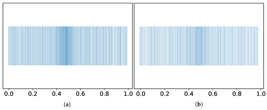
Figure 10.
Node distribution with (a) hard enforcement of boundary conditions and (b) loss-based enforcement.
Visually, the overall structure of the mesh in both cases is similar, with the node density adapted in the central region of the domain according to the control function. However, the exact boundary values reveal a key difference between the methods. When using the mask, the coordinates at the interval boundaries match the target values precisely: , . In contrast, when boundary conditions are enforced via the loss function, noticeable deviations are observed: , .
These results demonstrate that the use of the mask enables the strict enforcement of Dirichlet boundary conditions with machine precision, without the need to manually tune the penalty weights in the loss function. This is particularly important in problems requiring the exact placement of boundary nodes, such as in simulations with a prescribed geometry or fixed boundary values.
In the future, additional metrics will be used for a more detailed analysis of the differences between the numerical method and the PINN method. Specifically, quantitative grid deviation measures will be considered, such as the root mean square error between node coordinates, a smoothness measure of the node distribution, and PINN convergence indicators depending on various loss function parameters. This will allow for a more objective assessment of the accuracy and efficiency of each approach and help identify potential improvements in adaptive computational grid generation.
This section presents an analysis of the results for constructing a one-dimensional computational grid using both the numerical solution method and the PINN method. Cases with different numbers of control points defining node clustering zones are examined. An analysis of the node distribution, step size between neighboring points, coordinate differences, cumulative curves, and loss function shows that the PINN method produces smoother grids than the numerical method. As the number of control points increases, the differences between the methods become more pronounced. It is also observed that the convergence rate of the PINN method varies depending on the complexity of the problem, but the model successfully adapts to parameter changes. The obtained results provide insights into the applicability of PINNs for adaptive computational grid generation in numerical modeling tasks.
However, it should be noted that the numerical results used for comparison are not an absolute benchmark. The numerical method also contains approximation and discretization errors, which can influence the final node distribution. Therefore, a simple comparison with the numerical method cannot definitively determine the accuracy of the PINN approach but rather provides insight into the differences between the grid generation methods.
4. Conclusions
This study explored the problem of constructing one-dimensional computational grids using two approaches: the traditional numerical method and PINNs. The primary goal was to compare the accuracy, adaptability, and efficiency of these methods in solving the diffusion equation, which is used for adaptive grid generation. Testing was conducted with various control function parameters, allowing for a detailed analysis of the influence of and on the node distribution and the quality of the resulting computational grids.
The results of the numerical method demonstrated high accuracy in defining the grid structure, especially for small values of the parameter , which promoted more pronounced node clustering in regions requiring a detailed analysis. However, this method necessitated an explicit discrete solution of the equation, leading to increased computational costs, particularly as problem complexity grew. Additionally, the grid generated by the numerical method exhibited significant variations in the step size between nodes, which may require additional smoothing.
Conversely, the PINN method demonstrated a smoother node distribution, minimizing abrupt changes in the step size between neighboring points. The use of automatic differentiation in PyTorch enabled the seamless integration of the diffusion equation into the loss function, allowing the neural network model to learn while respecting physical constraints. Testing revealed that the PINN model was capable of adapting to different control function parameters; however, in some cases, deviations from the numerical solution were observed, particularly in regions with sharp gradients.
The convergence speed of the PINN model depends on optimization parameters and problem complexity. In some tests, a significantly higher number of iterations was required to achieve the desired accuracy, highlighting the need for the careful selection of optimal network hyperparameters. Additionally, an analysis of loss function graphs indicated that, as the number of control points increased, the training process became more complex, and the improvement in approximation accuracy was not uniform.
Additionally, this work investigated the implementation of hard boundary condition enforcement within the PINN framework using an embedded smooth mask function . Unlike traditional penalty-based approaches, this method ensures exact boundary values through architectural constraints, eliminating the need for loss weight tuning. Numerical tests confirmed that the use of this masking technique resulted in machine-precision boundary satisfaction, while the conventional loss-based approach led to notable deviations at the interval ends. This architectural enhancement improves physical consistency and can be especially beneficial for problems requiring strict boundary alignment.
Thus, the results of this study demonstrate that the PINN method can be used for adaptive computational grid generation, providing a smooth node distribution and flexible grid density adjustment. However, achieving high accuracy requires the careful selection of model parameters and the loss function. The numerical method remains a reliable tool for precise adaptive grid construction, especially in problems with sharp density variations. In the future, a hybrid approach combining the accuracy of the numerical method with the adaptability and generalization capabilities of neural network models could be developed.
Author Contributions
Conceptualization, O.T. and M.M.; methodology, M.M. and O.T.; software, M.M. and O.T.; validation, O.T., M.M. and D.A.-Z.; formal analysis, O.T.; investigation, M.M. and O.T.; resources, O.T.; data curation, M.M.; writing—original draft preparation, M.M.; writing—review and editing, O.T. and D.A.-Z.; visualization, M.M.; supervision, O.T. and D.A.-Z.; project administration, O.T.; funding acquisition, D.A.-Z. All authors have read and agreed to the published version of the manuscript.
Funding
This research was funded by the Committee of Science of the Ministry of Science and Higher Education of the Republic of Kazakhstan under grant funding for 2024–2026, number AP22688191.
Data Availability Statement
No new data were created or analyzed in this study.
Conflicts of Interest
The authors declare no conflicts of interest.
References
- Shokina, N.Y. Numerical simulation on adaptive grids of two-dimensional steady-state flows of liquid and gas. Comput. Technol. 1998, 3, 85–93. (In Russian) [Google Scholar]
- Thompson, J.F.; Soni, B.K.; Weatherill, N.P. (Eds.) Handbook of Grid Generation; CRC Press: Boca Raton, FL, USA, 1998. [Google Scholar] [CrossRef]
- Knupp, P.; Steinberg, S. Fundamentals of Grid Generation; CRC Press: Boca Raton, FL, USA, 1993. [Google Scholar] [CrossRef]
- Hsu, K.; Lee, S. A numerical technique for two-dimensional grid generation with grid control at all of the boundaries. J. Comput. Phys. 1991, 96, 451–469. [Google Scholar] [CrossRef]
- Thompson, J.F. Grid generation techniques in computational fluid dynamics. AIAA J. 1984, 22, 1505–1523. [Google Scholar] [CrossRef]
- Foster, I.; Kesselman, C. Computational grids. In Lecture Notes in Computer Science; Springer: Berlin/Heidelberg, Germany, 2001; pp. 3–37. [Google Scholar] [CrossRef]
- Liseikin, V.D. Review of structured adaptive grid generation methods. Comput. Math. Math. Phys. 1996, 36, 1–32. (In Russian) [Google Scholar]
- Skvortsov, A.V. Review of Delaunay triangulation algorithms. Comput. Methods Program. 2002, 3, 14–39. (In Russian) [Google Scholar]
- Skvortsov, A.V. Algorithms for constrained triangulation. Comput. Methods Program. 2002, 3, 82–92. (In Russian) [Google Scholar]
- Lebedev, A.S.; Liseikin, V.D.; Khakimzyanov, G.S. Development of adaptive mesh generation methods. Comput. Technol. 2002, 7, 29–43. [Google Scholar]
- Knupp, P.M. Algebraic mesh quality metrics. SIAM J. Sci. Comput. 2001, 23, 193–218. [Google Scholar] [CrossRef]
- Turar, O.N.; Akhmed-Zaki, D.Z. Design of adaptive unstructured grids using differential methods. J. Math. Mech. Comput. Sci. 2018, 98, 88–97. [Google Scholar] [CrossRef]
- Glasser, G.; Liseikin, V.; Shokin, Y.; Vaseva, I.; Likhanova, Y. Generation of Numerical Grids Through Beltrami and Diffusion Equations; Nauka: Novosibirsk, Russia, 2006. (In Russian) [Google Scholar]
- Liseikin, V.D.; Rychkov, A.D.; Kofanov, A.V. Applications of a comprehensive grid method to solution of three-dimensional boundary value problems. J. Comput. Phys. 2011, 230, 7755–7774. [Google Scholar] [CrossRef]
- Liseikin, V.D.; Kharitonchik, A.M.; Kofanov, A.V.; Likhanova, Y.V.; Vaseva, I.A. Application of Beltrami equations to generation of spatial adaptive grids. Russ. J. Numer. Anal. Math. Model. 2010, 25, 79–92. [Google Scholar] [CrossRef]
- Akhmed-Zaki, D.Z.; Turar, O.; Lebedev, D.V. Fragmented algorithm for adapted grid construction. Bull. Ser. Phys. Math. Sci. 2020, 71, 37–44. [Google Scholar] [CrossRef]
- Raissi, M.; Perdikaris, P.; Karniadakis, G.E. Physics-informed neural networks: A deep learning framework for solving forward and inverse problems involving nonlinear partial differential equations. J. Comput. Phys. 2019, 378, 686–707. [Google Scholar] [CrossRef]
- Lin, Q.; Zhang, C.; Meng, X.; Guo, Z. Monte Carlo Physics-informed neural networks for multiscale heat conduction via phonon Boltzmann transport equation. arXiv 2024, arXiv:2408.10965. [Google Scholar]
- Madir, B.-E.; Luddens, F.; Lothodé, C.; Danaila, I. Physics Informed Neural Networks for heat conduction with phase change. arXiv 2024, arXiv:2410.14216. [Google Scholar]
- Lawal, Z.K.; Yassin, H.; Lai, D.T.C.; Che Idris, A. Physics-informed neural network (PINN) evolution and beyond: A systematic literature review and bibliometric analysis. Big Data Cogn. Comput. 2022, 6, 140. [Google Scholar] [CrossRef]
- Haoteng, H.; Qi, L.; Chao, X. Physics-informed neural networks (PINN) for computational solid mechanics: Numerical frameworks and applications. Thin-Walled Struct. 2024, 205, 112495. [Google Scholar] [CrossRef]
- Meng, Z.; Qian, Q.; Xu, M.; Yu, B.; Yıldız, A.R.; Mirjalili, S. PINN-FORM: A new physics-informed neural network for reliability analysis with partial differential equation. Comput. Methods Appl. Mech. Eng. 2023, 414, 116172. [Google Scholar] [CrossRef]
- Kenzhebek, Y.; Amangeldiyev, A. Physics-informed neural networks for predicting pressure distribution in porous media. J. Probl. Comput. Sci. Inf. Technol. 2023, 1, 25–30. [Google Scholar] [CrossRef]
- Turar, O. Using PINN to solve equations of equidistributional method for constructing 2D structured adapted numerical grids. J. Probl. Comput. Sci. Inf. Technol. 2023, 1, 28–33. [Google Scholar] [CrossRef]
- Pelissier, U.; Parret-Fréaud, A.; Bordeu, F.; Mesri, Y. Graph neural networks for mesh generation and adaptation in structural and fluid mechanics. Mathematics 2024, 12, 2933. [Google Scholar] [CrossRef]
- Bohn, C.-A. A neural network-based finite element grid generation algorithm for the simulation of light propagation. Appl. Numer. Math. 2003, 46, 263–277. [Google Scholar] [CrossRef]
- Chen, X.; Liu, J.; Zhang, Q.; Liu, J.; Wang, Q.; Liang, D.; Pang, Y. Developing a novel structured mesh generation method based on deep neural networks. Phys. Fluids 2023, 35, 097137. [Google Scholar] [CrossRef]
- Zhou, Y.; Wang, Y.; Liu, Y. PINN-MG: A physics-informed neural network for mesh generation. arXiv 2025, arXiv:2503.00814. [Google Scholar]
- Chen, X.; Liu, J.; Yan, J.; Wang, Z.; Gong, C. An Improved Structured Mesh Generation Method Based on Physics-informed Neural Networks. arXiv 2022, arXiv:2210.09546. [Google Scholar] [CrossRef]
- Sukumar, N.; Srivastava, A. Exact imposition of boundary conditions with distance functions in physics-informed deep neural networks. Comput. Methods Appl. Mech. Eng. 2022, 389, 114333. [Google Scholar] [CrossRef]
- Sokolovskyy, Y.; Manokhin, D.; Kaplunsky, Y.; Mokrytska, O. Development of software and algorithms of parallel learning of artificial neural networks using CUDA technologies. Technol. Audit Prod. Reserves 2021, 5, 21–25. [Google Scholar] [CrossRef]
Disclaimer/Publisher’s Note: The statements, opinions and data contained in all publications are solely those of the individual author(s) and contributor(s) and not of MDPI and/or the editor(s). MDPI and/or the editor(s) disclaim responsibility for any injury to people or property resulting from any ideas, methods, instructions or products referred to in the content. |
© 2025 by the authors. Licensee MDPI, Basel, Switzerland. This article is an open access article distributed under the terms and conditions of the Creative Commons Attribution (CC BY) license (https://creativecommons.org/licenses/by/4.0/).