Abstract
We address the challenge of efficiently approximating piecewise smooth functions, particularly those with jump discontinuities. Given function values on a uniform grid over a domain in , we present a novel B-spline-based approximation framework, using new adaptable quasi-interpolation operators. This approach integrates discontinuity detection techniques, allowing the quasi-interpolation operator to selectively use points from only one side of a discontinuity in both one- and two-dimensional cases. Among a range of candidate operators, the most suitable quasi-interpolation scheme is chosen to ensure high approximation accuracy and efficiency, while effectively suppressing spurious oscillations in the vicinity of discontinuities.
1. Introduction
The development of approximation methods for piecewise smooth functions was originally motivated by the need to solve hyperbolic partial differential equations with discontinuous solutions [1,2]. In more recent years, these methods have found applications in areas such as image processing and non-smooth optimization.
The Weighted Essentially Non-Oscillatory (WENO) method builds upon the Essentially Non-Oscillatory (ENO) scheme [3], aiming to achieve high-order accuracy in smooth regions while preventing spurious oscillations near discontinuities in the solution of conservation laws.
The WENO method is founded on the principle that, to approximate a discontinuous function accurately, one should use data only from one side of the discontinuity. This approach ensures that, when approximating the function at a given point, the function data are drawn exclusively from the smooth region surrounding that point, without incorporating values from both sides of the discontinuity. Various techniques are employed to assess the function’s smoothness and prevent the use of data across discontinuities.
The WENO method was first introduced in [3,4]. Later, Ref. [2] refined the approach by incorporating a local nonlinear convex combination of multiple interpolants spanning different stencils. In this method, the weights are computed based on smoothness indicators within each stencil. Ref. [1] further improved the smoothness indicators by incorporating a measure derived from total variation, leading to enhanced accuracy. The WENO algorithm has since been widely studied and applied in various works, including [5,6,7].
More recent advancements and algorithms based on the WENO framework can be found in [8,9,10,11,12,13] and many other studies.
This paper introduces an approximation method for discontinuous functions based on their values sampled on a uniform grid over a domain . The proposed approach is a WENO-like algorithm that utilizes B-spline quasi-interpolation operators. A key advantage of this method is its computational efficiency, as it is both fast and local.
The resulting approximation inherits the smoothness of B-splines, achieving a high order of accuracy in smooth regions. For example, when using cubic B-splines, the approximation achieves overall smoothness and an approximation order in smooth regions. Moreover, it remains non-oscillatory near function discontinuities, providing stability and accuracy, which are essential for applications in non-smooth optimization.
Another notable advantage of the method is its natural extension to higher dimensions. We begin by presenting the algorithm in one dimension and subsequently generalize it to two dimensions, introducing an automatic stencil selection strategy to handle quasi-interpolation near singularity curves.
This paper is structured as follows. Section 2 outlines the theoretical foundations of quasi-interpolation. Section 3 describes the construction and application of an adapted cubic spline quasi-interpolation scheme for non-smooth univariate functions. In Section 4, we extend the approach to the bivariate setting, incorporating a mechanism for handling discontinuities across unknown curves, and demonstrate its effectiveness through theoretical results and numerical experiments.
2. Preliminaries
In this paper, we present an approximation method for a non-smooth function , defined on a domain , based on its known values at a uniform grid , where . The proposed approximation is constructed using a quasi-interpolation approach, expressed as
where denotes the basis functions of the quasi-interpolation operator. In [14], we introduced a method for constructing basis functions for quasi-interpolation approximation based on Box-Splines in . In [14], we outlined two key properties that the basis functions for quasi-interpolation should satisfy:
- 1.
- Polynomial reproduction:
- 2.
- Compact support:
Here, denotes the open ball of radius r centered at a, and h is the fill-distance of the point-set A, that is, the radius of the largest open ball centered in that does not contain any point from A. R is independent of and h.
In [14], we presented the following proposition.
Proposition 1.
In the one-dimensional setting, Speleers in [15] presented a comprehensive analysis of spline quasi-interpolation operators on uniform grids. The simplest quasi-interpolation operator is the Schoenberg operator defined by
where denotes the centered B-spline of degree , supported on the interval with nodes . The Schoenberg operator achieves an approximation order of for smooth functions. When applied to functions with jump discontinuities, it produces a smooth transition between the continuous regions without introducing overshoots or oscillations, thereby avoiding Gibbs-like phenomena.
An improved approximation order of , can be achieved using the following quasi-interpolation operator based on cubic B-splines on a uniform grid:
This operator can also be expressed in form (1) using the basis functions
Thanks to its locality and its exact reproduction of polynomials of a degree up to three, the operator achieves an approximation order of for functions that are -smooth. However, when applied to functions with jump discontinuities, it tends to introduce oscillations and Gibbs-like overshoots near the discontinuity. The term Gibbs-like overshoot refers to spurious oscillations in the approximation near a jump, characterized by the persistence of their magnitude even as ; see [16].
This paper aims to identify quasi-interpolation operators that achieve high-order accuracy in smooth regions while remaining free of overshoots near jump discontinuities.
3. Constructing Quasi-Interpolation Operators for Approximating Non-Smooth Functions in
Let the domain and let X be the set of grid points uniformly spaced in : . . After rearranging the indices, the quasi-interpolation operator (7) can be expressed as follows:
We refer to this operator as the symmetric quasi-interpolation operator.
The central idea of this paper is to define a quasi-interpolation operator that utilizes alternative combinations of function values, distinct from those in (9), while still preserving the ability to reproduce cubic polynomials and achieving an approximation order. The goal is to construct a quasi-interpolation operator that uses only function values from one side of a discontinuity, ensuring both accuracy and the avoidance of spurious oscillations.
We begin by formulating a forward quasi-interpolation operator in a non-symmetric form:
To ensure the desired property of reproducing cubic polynomials, we derive a system of equations for unknowns , and D:
for . Since the space of polynomials is shift-invariant, it is sufficient to consider the equation for . Solving this system of equations, we obtain the quasi-interpolation operator :
Similarly, we can construct a backward quasi-interpolation operator that relies only on function values to the left of . This leads to the formulation of :
After establishing quasi-interpolation operators (9), (12), and (13), we introduce a general mixed quasi-interpolation operator, expressed as
where the weights are selected from the following three options:
Proposition 2.
Let , . Consider the operator defined in (14), where the weights are chosen arbitrarily from the three available options: , , or . Then, the approximation error satisfies
Proof.
From relation (11), it follows that reproduces , the space of cubic polynomials. This reproduction property, together with the compact support property of , directly implies the stated result. □
3.1. Using the Smoothness Indicator to Define a New Adapted Approximation
Returning to the problem of approximating a piecewise smooth function, we now describe the method for selecting the appropriate weight at each location .
The first step is to identify the interval containing the discontinuity. This is achieved using the following approach, assuming a uniform grid:
For each point , we compute a smoothness indicator :
where is the central second difference, defined as
The value of is of size at smooth regions of f, and O(1) if contains a discontinuity of f. Consequently, large values of indicate regions of significant variation and are useful for detecting discontinuous intervals. We use second-order differences, rather than first-order, to also capture singularities such as jumps in the first derivative.
If exceeds a predetermined threshold, we conclude that a discontinuity exists within the interval . Once the interval of discontinuity is identified, we apply quasi-interpolation operator (14) while ensuring that the discontinuous region is excluded.
We select the weights in quasi-interpolation operator (14) from the three available options (15)–(17), so that the resulting operator depends only on function values from one side of a discontinuity. The selection is carried out as follows:
For each , we compute the three values,
Let be the index for which is minimal. We then set in (14). Notably, the procedure naturally selects in smooth regions.
The resulting modified operator is referred to as the adapted quasi-interpolation operator, denoted by .
3.2. Theoretical Considerations of the Adapted Approximation
The following propositions quantify the overshoots produced by the symmetric quasi-interpolation operator and establish that the adapted quasi-interpolation operator eliminates such overshoots.
Let f be a non-smooth function defined by
where , . Let D denote the size of the jump discontinuity at , defined by . Consider the quasi-interpolation approximations and , constructed using the sampled data .
Proposition 3.
For any , there exist points and such that
Proof.
Since is a linear operator, it suffices to prove the result for the function
which corresponds to the case and , and yields .
Proposition 4.
Proof.
First, assume , and h to be sufficiently small. Then, by construction, each of the weights selected for the adapted quasi-interpolation operator uses only function values from one side of the jump discontinuity at . Error estimate (21) follows by considering the support of and the reproduction of cubic polynomials by for .
Next, we observe that each of the candidate weights, , , and , satisfies the approximation property
provided that the corresponding weights are constructed using only function values from one side of the jump discontinuity. This is readily verified in the case of , as it is symmetric and centered and reproduces linear polynomials. For , the approximation property in (22) also holds, as a direct consequence of the defining relation (11). Thus, in particular in , we have
3.3. Numerical Results in One Dimension
We applied the adapted quasi-interpolation method to two distinct non-smooth test functions.
The first test function is
The second test function is
The available data consist of sampled values of the non-smooth test functions at uniformly spaced points , . Figure 1 and Figure 2 illustrate the two test functions.
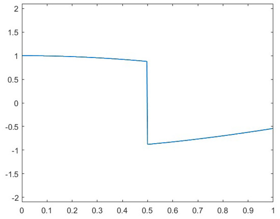
Figure 1.
Test function .
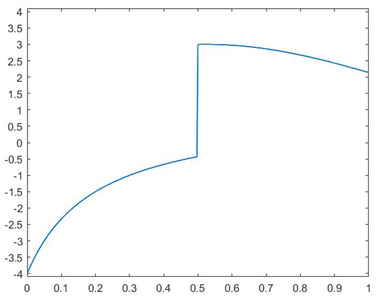
Figure 2.
Test function .
Representative numerical results, which support the theoretical claims established in the preceding propositions, are shown in Figure 3 and Figure 4 for the first test function and Figure 5 and Figure 6 for the second test function .
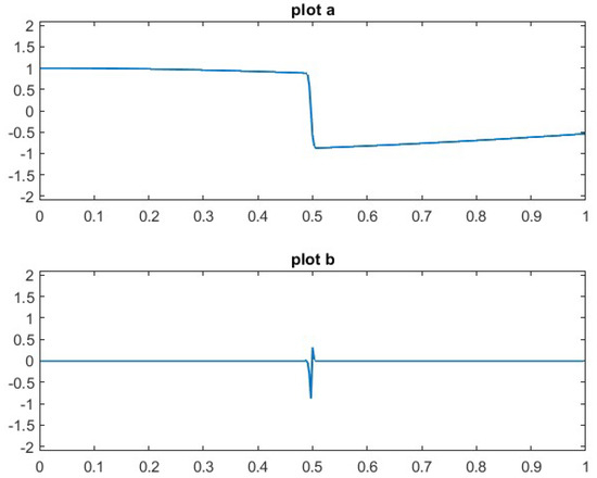
Figure 3.
Plot a: The adapted quasi-interpolation approximation of . Plot b: The error in the approximation.
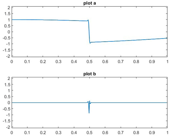
Figure 4.
Plot a: Symmetric quasi-interpolation approximation of . Plot b: Approximation error of the symmetric quasi-interpolation.
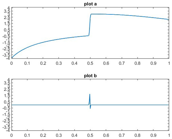
Figure 5.
Plot a: The adapted quasi-interpolation approximation of . Plot b: The approximation error.
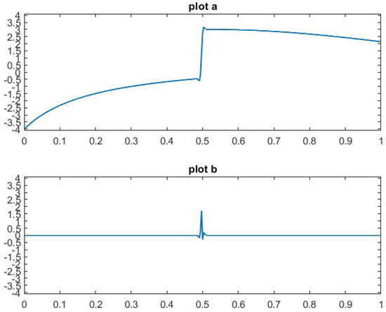
Figure 6.
Plot a: Symmetric quasi-interpolation approximation of . Plot b: Approximation error of the symmetric quasi-interpolation.
A comparison between the graphs in Figure 3, which display the results of the adapted quasi-interpolation method, and those in Figure 4, obtained using the symmetric quasi-interpolation, reveals a significant difference. The Gibbs-like oscillations and overshoots near the discontinuity, clearly present in Figure 4, are entirely eliminated in the adapted approach shown in Figure 3. This qualitative improvement is further corroborated by the behavior of the approximation error, as illustrated in the lower panels of Figure 3 and Figure 4. The corresponding results for the second test function are presented in Figure 5 and Figure 6.
4. Adapted Quasi Interpolation Operators for Non-Smooth Functions in R2
Consider a discontinuous piecewise smooth function f defined in . Let be a smooth curve that separates into two domains and , and suppose that
with and . Assume that is given on the grid points in , , , and define .
We wish to approximate the function using a quasi-interpolation operator of the form
Similarly to the one-dimensional case, the weights are defined as linear combinations of the given function values, ensuring that the operator Q reproduces cubic polynomials. There are several options for defining the weights . For a smooth function f, the optimal choice is to use the cross product of the one-dimensional symmetric quasi-interpolation operator (9). However, in the case of non-smooth function approximation, we must ensure that does not depend on function values from both sides of the singularity curve .
In the following, we describe the method for computing the weights in (27). This is achieved by taking the tensor product of the one-dimensional quasi-interpolation operators , , and as defined in (15)–(17), respectively. This construction yields a total of nine two-dimensional quasi-interpolation operators:
where and denote the symmetric one-dimensional quasi-interpolation operators in the and directions, respectively; and represent the forward operators; and and , the backward ones. If we denote the identity operator by I, by , the forward operator in the x direction is , and by , the forward operator in the y direction is . We obtain nine cross products of the three quasi-interpolation operators in one dimension. For example,
which gives
Similarly, we define the remaining eight quasi-interpolation operators in two dimensions. To compute the weights in (27), we consider the nine quasi-interpolation operators outlined in (28). Each operator uses a distinct stencil of data values from the grid for its calculations. For example, the operator in (29) incorporates 16 points:
4.1. Smoothness Indicator and the New Adapted Approximation in 2D
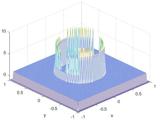
In the two-dimensional case, the smoothness indicator is based upon the absolute value of the discrete four-direction Laplacian:
We note that if all the values involved in (31) lie within a smooth region of f, then as . However, if incorporates values of f from both sides of the singularity curve , then . Figure 7 presents the values of the smoothness indicator corresponding to the non-smooth test function defined in Equation (39).
For each of the nine quasi-interpolation operators in (28), we attach a smoothness indicator by summing Laplacian values as follows:
Each of the nine quasi-interpolation operators is computed using the values of f on a rectangular stencil of indices:
The corresponding smoothness indicator is defined as
Thus, for each grid point , we compute nine values, , corresponding to the above nine quasi-interpolation operators , applied using their respective stencils. From these, we select the minimum value, denoted as
and assign the associated weight to the point .
Once the weights are computed, they are inserted into the quasi-interpolation scheme defined in (27). The resulting approximation operator is referred to as the adapted quasi-interpolation operator, and is denoted as .
4.2. Theoretical Results for the 2D Adapted Approximation
Similarly to one-dimensional Proposition 2, we obtain the following proposition for the two-dimensional case.
Proposition 5.
Proposition 6.
Let f be a piecewise function defined as in (26), with a singularity curve Γ. Then, the symmetric quasi-interpolation approximation defined above is globally , and it satisfies the error estimate
where C is a constant independent of h. Near the discontinuity at Γ, the approximation exhibits some Gibbs-like overshoots.
Proof.
Observe that the support of the basis function is the Cartesian product of the supports of and , each of which spans an interval of length 4. Consequently, the diameter of the two-dimensional support is . Moreover, the weights in the symmetric scheme involve function values located at a distance up to from the grid point . Depending on the local orientation of the singularity curve , it follows that at points satisfying the condition in (35), the symmetric approximation accesses only values from one side of . Thus, the error estimate given in (35) follows as a direct consequence of the support structure and the localized nature of the approximation. The occurrence of Gibbs-like overshoots can be demonstrated using arguments analogous to those in the univariate case, as outlined in Proposition 3. In particular, near portions of that are aligned with one of the coordinate axes, the overshoots are identical to those observed in the univariate setting. □
The following proposition shows that the adapted quasi-interpolation operator extends the region over which optimal approximation accuracy is attained, while eliminating Gibbs-like overshoots near discontinuities.
Proposition 7.
Let f be a piecewise function defined as in (26), with a smooth singularity curve Γ. Then, the adapted quasi-interpolation approximation defined above is globally , and, for sufficiently small h, it satisfies the error estimate
where C is a constant independent of h. Moreover, the approximation does not exhibit any Gibbs-like overshoots near the discontinuity at Γ.
Proof.
First, assume a non-zero jump across , and h is sufficiently small. Then, by construction, each of the weights selected for the adapted quasi-interpolation operator uses only function values from one side of the jump discontinuity at . Error estimate (36) follows by considering the support of and the reproduction of cubic polynomials by .
Next, we observe that each of the nine candidate weights, , satisfies the approximation property
This follows directly from the fact that each weight is constructed as a tensor product of two univariate weights, each of which satisfies the one-dimensional approximation property given in (22).
Thus, we have
4.3. Numerical Results for Non-Smooth Functions in Two Dimensions
We applied both the symmetric and the newly adapted quasi-interpolation methods, as described in Section 4, to discontinuous functions of the form given in Equation (26).
The results for a representative test function, illustrated in Figure 8, are presented below. This function is defined as follows:
We refer the reader to Figure 7, which presents the values of the smoothness indicator corresponding to this test function. The numerical results presented in Figure 9 and Figure 10 provide strong support for the theoretical findings established in Propositions 6 and 7. Specifically, Figure 10 illustrates the shortcomings of the symmetric quasi-interpolation approach, exhibiting noticeable Gibbs-like overshoots and spurious oscillations near the discontinuity. In contrast, these artifacts are effectively eliminated by the newly adapted quasi-interpolation operator, as demonstrated in Figure 9. All results were obtained using a grid spacing of .
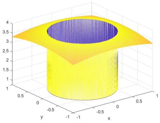
Figure 8.
The test function defined by (39).
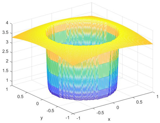
Figure 9.
The adapted quasi-interpolation approximation.
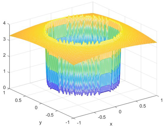
Figure 10.
The approximation using symmetric quasi-interpolation.
5. Conclusions
Quasi-interpolation algorithms are powerful tools for generating smooth and intricate curves and surfaces, making them highly valuable in computer graphics and geometric modeling. These methods are direct, yielding high-order smooth approximations without requiring the solution of linear systems or iterative procedures. However, standard quasi-interpolation schemes are generally ineffective when approximating non-smooth functions, particularly those with discontinuities.
In this work, we propose a novel adapted quasi-interpolation operator designed for the approximation of univariate and bivariate functions exhibiting jump singularities. We provide theoretical justification and support our claims with numerical experiments, demonstrating that the new method produces smooth approximations that avoid Gibbs-like oscillations near discontinuities.
Moreover, the construction of the proposed operator naturally extends to higher dimensions. For instance, it can be applied to approximate three-dimensional functions with discontinuities across unknown surfaces, while maintaining high approximation quality.
Author Contributions
Methodology, D.L.; software, N.G. All authors have read and agreed to the published version of the manuscript.
Funding
This research received no external funding.
Data Availability Statement
The original contributions presented in this study are included in the article. Further inquiries can be directed to the corresponding author.
Conflicts of Interest
The authors declare no conflict of interest.
References
- Jiang, G.; Shu, C.-W. Efficient Implementation of Weighted ENO Schemes. J. Comput. Phys. 1996, 126, 202–228. [Google Scholar] [CrossRef]
- Liu, X.D.; Osher, S.; Chan, T. Weighted essentially nonoscillatory schemes. J. Comput. Phys. 1994, 115, 200–212. [Google Scholar] [CrossRef]
- Harten, A.; Engquist, B.; Osher, S.; Chakravarthy, S.R. Uniformly high order accurate essentially non-oscillatory schemes, III. J. Comput. Phys. 1987, 71, 231–303. [Google Scholar] [CrossRef]
- Harten, A.; Osher, S. Uniformly high order accurate nonoscillatory schemes, I. SIAM J. Numer. Anal. 1987, 24, 279–309. [Google Scholar] [CrossRef]
- Shu, C.W. High Order ENO and WENO Schemes for Computational Fluid Dynamics; Springer: Berlin/Heidelberg, Germany, 1999; pp. 439–582. [Google Scholar]
- Arandiga, F.; Baeza, A.; Belda, M.; Mulet, P. Analysis of WENO schemes for full and global accuracy. SIAM J. Numer. Anal. 2011, 49, 893–915. [Google Scholar] [CrossRef]
- Henrick, A.K.; Aslam, T.D.; Powers, J.M. Mapped weighted essentially non-oscillatory schemes: Achieving optimal order near critical points. J. Comput. Phys. 2005, 207, 542–567. [Google Scholar] [CrossRef]
- Amat, S.; Levin, D.; Ruiz, J.; Yanez, F. A new B-Spline type approximation method for non-smooth functions. App. Math. Lett. 2023, 141, 108628. [Google Scholar] [CrossRef]
- Amat, S.; Levin, D.; Ruiz, J.; Yanez, D.F. Explicit multivariate approximations from cell-average data. Adv. Comput. Math. 2022, 48, 85. [Google Scholar] [CrossRef]
- Amat, S.; Ruiz, J. New WENO smoothness indicators computationally efficient in presence of corner discontinuities. J. Sci. Comput. 2017, 71, 1265–1302. [Google Scholar] [CrossRef]
- Arandiga, F.; Belda, A.M.; Mulet, P. Point-Value WENO Multiresolution Applications to Stable Image Compression. J. Sci. Comput. 2010, 43, 158–182. [Google Scholar] [CrossRef]
- Arandiga, F.; Donat, R.; Lopez-Urena, S. Nonlineaer inprovements of quasi-interpolating splines to approximate piecewise smooth functions. Appl. Math. and Comput. 2023, 448, 127946. [Google Scholar]
- Amat, S.; Levin, D.; Ruiz-Álvarez, J.; Yanez, D.F. Non-linear WENO B-spline based approximation method. Numer. Algorithms 2025, 98, 1141–1169. [Google Scholar] [CrossRef]
- Gruberger, N.; Levin, D. Basis functions for Scattered Data Quasi-Interpolation. In Proceedings of the Curves and Surfaces: 8th International Conference, Paris, France, 12–18 June 2014; Springer International Publishing: Berlin/Heidelberg, Germany, 2015; pp. 263–271. [Google Scholar]
- Speleers, H. Hierarchical spline spaces: Quasi-interpolants and local approximation estimates. Adv. Comput. Math. 2017, 43, 235–255. [Google Scholar] [CrossRef]
- Gibbs, J.W. Fourier’s Series. Nature 1899, 59, 1522. [Google Scholar] [CrossRef]
Disclaimer/Publisher’s Note: The statements, opinions and data contained in all publications are solely those of the individual author(s) and contributor(s) and not of MDPI and/or the editor(s). MDPI and/or the editor(s) disclaim responsibility for any injury to people or property resulting from any ideas, methods, instructions or products referred to in the content. |
© 2025 by the authors. Licensee MDPI, Basel, Switzerland. This article is an open access article distributed under the terms and conditions of the Creative Commons Attribution (CC BY) license (https://creativecommons.org/licenses/by/4.0/).