Article

Improved Asynchronous Federated Learning for Data Injection Pollution

1
School of Information Engineering, Minxi Vocational & Technical College, Longyan 364000, China
2
School of Mathematics and Information Engineering, Longyan University, Longyan 364000, China
3
Department of Automation, Xiamen University, Xiamen 361000, China
*
Author to whom correspondence should be addressed.
Algorithms 2025, 18(6), 313; https://doi.org/10.3390/a18060313
Submission received: 23 March 2025 / Revised: 30 April 2025 / Accepted: 20 May 2025 / Published: 26 May 2025
(This article belongs to the Section Evolutionary Algorithms and Machine Learning)

Abstract

:
In view of the problems of data pollution, incomplete feature extraction, and poor multi-network parameter sharing and transmission under the federated learning framework of deep learning, this article proposes an improved asynchronous federated learning algorithm of multi-model fusion based on data injection pollution. Through data augmentation, the existing dataset is preprocessed to enhance the algorithm’s ability to identify the noise data. In our approach, the residual network is used to extract the static information of the image, the capsule network is used to extract the spatial dependence among the internal structures of the image, several layers of convolution are used to reduce the dimensions of both features, and the two extracted features are fused. In order to reduce the transmission overhead of parameters shared between the residual network and capsule network, we adopt an asynchronous parameter transmission between the global trainer and the local trainer. When the global trainer broadcasts the parameters to each local trainer, several trainers are randomly selected to avoid communication link blockage. Finally, through conducting various experiments, the results show that our alogrithm can effectively extract the pathological features in the image and achieve higher accuracy, outperforming the current mainstream algorithms.

1. Introduction

In recent years, the rapid development of distributed machine learning has increased the attention paid to Federated Learning (FL), which is a collaborative learning framework for privacy protection. Unlike traditional centralized learning models, federated learning allows for multiple participants to train the model locally and update the global model parameters without sharing the raw data. However, in practice, synchronous federated learning often faces problems such as differences in computing power, network latency, and device availability, which require all participants to participate in each iteration simultaneously. To meet these challenges, Asynchronous Federated Learning (AFL) has gradually become a research focus.
Aynchronous federated learning allows for different clients to update the global model parameters at different frequencies at different times, thus improving the flexibility and efficiency of the system. Compared with synchronization methods, asynchronous methods can better adapt to computational power and network conditions of different devices, while reducing the impact of clients with a longer waiting time on the overall training schedule. In recent years, the research has mainly focused on the following aspects:
(1) Optimization of the algorithm design using an adaptive aggregation strategy: We proposed a variety of adaptive aggregation methods, such as FedAvg based on a weighted average [1], and its improved version, to improve the speed and robustness of model convergence by dynamically adjusting the weight of the client’s contribution. Asynchronous gradient descent methods and asynchronous optimization algorithms based on SGD (stochastic gradient descent), such as Async-SGD [2] and its variants, have been widely studied. These algorithms significantly improve the training efficiency by parallelizing the training tasks of the client and the parameter-updating process of the server.
(2) Privacy protection mechanism: In AFL, communication latency can lead to data from some clients being used multiple times, increasing the risk of privacy leakages. For this problem, the researchers proposed a method based on differential privacy [3] and homomorphism encryption [4] to ensure the privacy of client data. In response to model theft attacks and intermediate results leakage, some work combines federated learning and federated enhanced learning [5] to further improve security in an asynchronous environment.
(3) Model heterogeneity treatment: Clients in AFL often have different computational powers and data distribution rates, leading to inconsistencies in model updates. To this end, the researchers proposed [6], a method based on federated meta-learning, to balance the contributions of different clients by introducing a meta-optimizer to the server side. In addition, for the data heterogeneity problem, some work uses task-decomposition-based methods, such as FedMD [7] and Task-Aware FL [8], to decompose global tasks into multiple subtasks and assign them to different clients.
(4) Scalability and fault tolerance: To improve the scalability of AFL, researchers proposed the hierarchical federated learning framework [9], which effectively reduces communication latency and reduces bandwidth consumption by adding intermediate server nodes. In terms of fault tolerance, some work explores how to handle client drops or long unresponsive cases, such as the retransmission mechanism based on timeout detection [10] and the redundant backup policy [11].
(5) Practical application and exploration: AFL has been widely used in multiple fields, such as Medical Data Collaboration [12], recommended system [13], and edge computing [14]. The heterogeneity of the devices and the complexity of the network environment in these application scenarios further promote research on and the development of asynchronous methods. In recent years, federated learning has emerged as a revolutionary approach, addressing challenges related to data privacy, security, and distributed data silos across various domains. In the realm of traffic control, the advent of intelligent transportation systems has brought about a new era of traffic management [15]. Traffic signal control (TSC) is a crucial aspect of this, aiming to mitigate congestion, reduce travel time, and cut down on emissions and energy consumption. Reinforcement learning (RL) has been a primary technique for TSC. However, traditional centralized learning models face significant communication and computing bottlenecks, while distributed learning struggles to adapt across different intersections. As proposed by Bao et al. [16], federated learning provides a novel solution. It integrates the knowledge of local agents into a global model, overcoming the variations among intersections through a unified agent state structure. The model aggregates a segment of the RL neural network to the cloud, and the remaining layers undergo fine-tuning during the convergence of the training process. Experiments have demonstrated a reduction in queuing and waiting times globally, and the model’s scalability has been validated on a real-world traffic network in Monaco. In the field of image processing, federated learning has also shown great potential. With the increasing generation of image data from diverse sources, such as surveillance cameras, medical imaging devices, and mobile applications, data privacy becomes a major concern. Federated learning allows for edge devices or local servers to train models on their local data without sharing the raw data, thus safeguarding privacy. As elaborated in the review paper “A review on federated learning towards image processing” by Khokhar et al. [17], federated learning in image processing can be applied to various tasks like image recognition, segmentation, and classification. For example, in medical image segmentation across multiple healthcare centers, each center can train a model on its local patient data, and then the model parameters are aggregated to build a global model that can be beneficial for all participating centers while protecting patient privacy [18]. The applications of federated learning in traffic control and image processing are still in the process of continuous exploration and development. As technology advances, more innovative applications and optimized algorithms are expected to emerge, further enhancing the efficiency and effectiveness of these two important fields.
Although asynchronous federal learning has made remarkable progress in recent years, there are still some challenges, as follows [19,20,21]:
(1) Communication efficiency: The asynchronous method can lead to conflicts between parameter updates on the server side. Recent studies such as [22] have explored dynamic communication scheduling to mitigate such conflicts. However, how to effectively and orderly coordinate communication between the client and the server in heterogeneous environments remains an open problem that must urgently be solved.
(2) Convergence guarantee: Most existing studies are based on experimental verification and lack rigorous theoretical analysis and proof of convergence.
(3) Robustness: Malicious attacks in the asynchronous environment (such as model poisoning) may have a serious impact on the global model. Recent work [23] proposed the use of gradient anomaly detection frameworks to filter poison updates, but the integration of such methods into AFL requires further investigation. How to effectively improve the anti-attack ability of the system remains an important direction of future research.
In general, AFL, a flexible and efficient distributed learning method, shows great potential in the protection of privacy and in scenarios with limited computing resources. With the development of theoretical research and technical practice, its performance in practical applications will improve. In the massive data-driven machine learning method, the data pollution problem inevitably affects the robustness of the model, leading to learning shock and an insufficient prediction ability. However, through establishing a complete data cleaning process, adopting an anomaly detection algorithm, and establishing a data-quality evaluation system, the model can improve its tolerance of data pollution faults, thus improving its robustness. Under the federated learning framework, there are two main sources of data pollution:
(1) Incontamination of raw data: This kind of pollution is relatively common. For classification and regression models, the cause of data pollution may be the change in sample distribution or disordered sample labeling. When the original data are contaminated, the detection and filtering of contaminated samples become the focus of research. Whether abnormal samples can be detected quickly and effectively is crucial to the training of machine learning models.
(2) Contamination generated during data transmission: In the federal learning framework, there is frequent data transfer between global trainers and the local trainers, which can easily produce pollution in the process of data transmission. When the trainer uploads gradient pollution, the upload gradient security aggregation from the global trainer to the local trainers is prone to improper aggregation and algorithm training shock, and may even fail to converge. In this case, the parameters are broadcast to the local trainers, leading to the pollution of the model parameters under the federal framework.
In conclusion, this article studies an important AFL issue:how to detect gradient anomalies in a data pollution environment—and proposes an improved algorithm named Asynchronous Federated Learning Improving (AFLI), which focuses on the impact of data injection contamination on gradient information.
The main work and contributions of this article are as follows:
(1) When the original data are contaminated, it is difficult for the local trainer to accurately identify and filter the data, which transfers the parameter gradient of the abnormal data to the global trainer and then causes the systematic parameter pollution problem. In this article, we preprocess existing datasets to improve the ability of the algorithm to identify noise data.
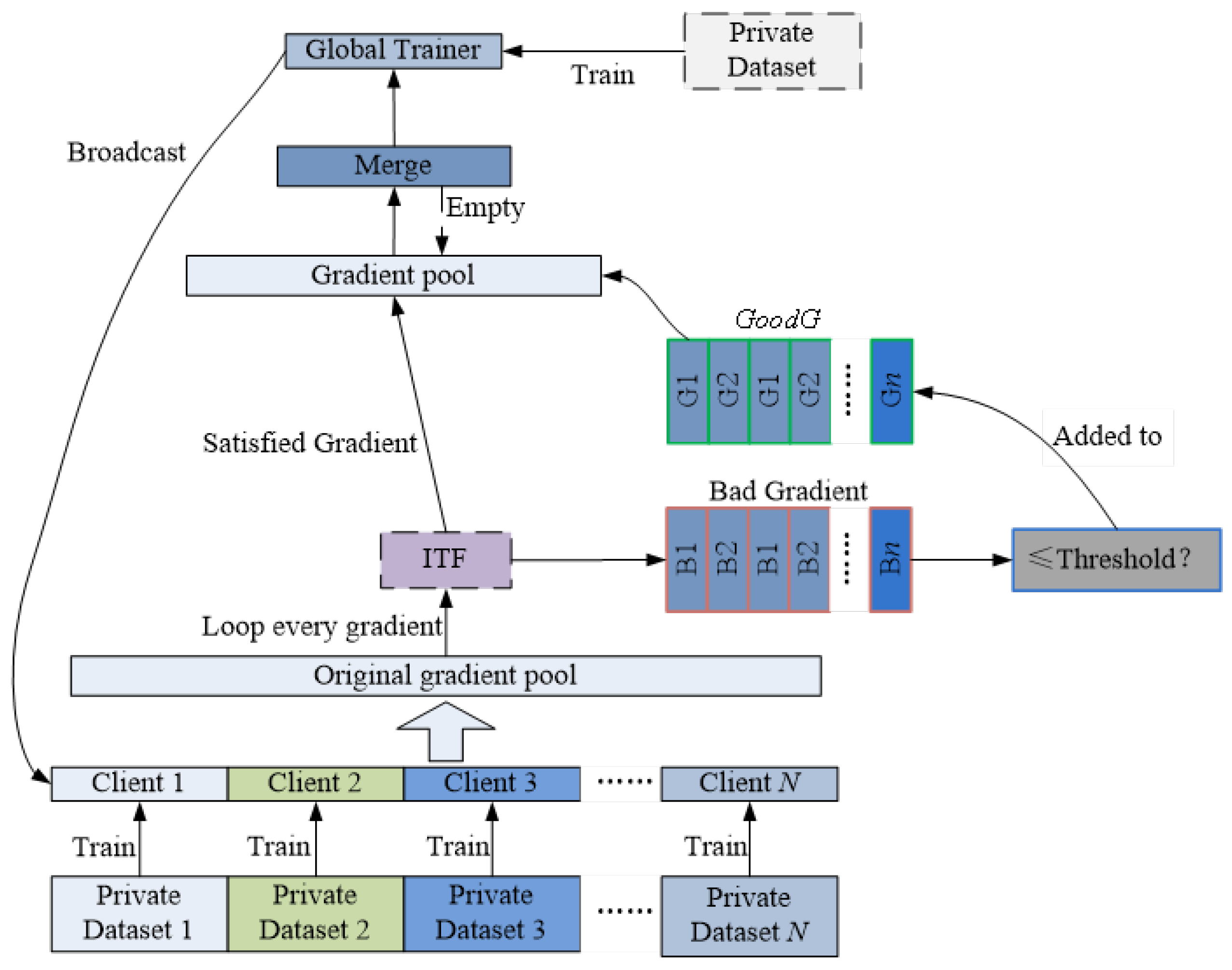
(2) An anomaly detection algorithm is used during the gradient transmission process. There is frequent transmission of parameters between the local trainer and the global trainer. When the local trainer transfers its own gradient to the global trainer, severe gradient contamination will cause the global trainer to effectively update the parameters. In order to solve this problem, this article mainly adopts two methods: first, the gradient is uploaded by each local trainer through the experience pool technology; second, the ITF (Isolation Forest) algorithm is used to detect and eliminate the abnormal gradient, and only the normal gradients are used to update the parameters of the global trainer to effectively alleviate the influence of the abnormal gradient on the parameter update.
(3) Based on previous work, this article achieved relatively high accuracy in two data sets, including two CLS and ZXSFL. Various experiments demonstrate that the algorithm can effectively detect contaminated data sets and achieve high accuracy.

2. Explanation of the Meanings of the Symbols

This article will provide an overview of the parameters of the mathematical formulas involved and provide the corresponding explanations. The parameters calculated using each formula will be explained in the formula interpretation section and will not be repeated in this section. The definitions of each variable are detailed in Table 1.
k = 0 , Global Trainer k , k > 0 , Client Trainer
where k greater than 0 represents the number of the local trainer and k less than or equal to 0 represents the global trainer.
In Table 1, the RSA encryption algorithm encrypted the parameters. Whenever a parameter transfer occurs between trainers, the RSA algorithm is triggered to perform encryption operations. RSA encryption algorithms vary in different dimensions, resulting in differences in encryption speed and the results. In this study, the lowest-dimensional RSA encryption algorithm was selected to encrypt the data; parameter En represents the RSA encryption process.
The parameters are the concept of training cycles. Training is terminated once the number of iterations of the private dataset is reached. It should be noted that private data sets vary in size, so the time needed to reach the established training cycle will vary. Training stops when the number of iterations of trainer k reaches a predetermined threshold, but the trainer can still continue to receive parameter updates from the global trainer provided that the conditions of Equation (2) are satisfied.
recept k = True , if loss or accuracy satisfy threshold False , otherwise
In Equation (2), the data exchange with other trainers in the federated framework stops if and only if the test’s precision or the loss of trainer k reaches the specified threshold. T e k is the number of iterations of trainer k in each cycle T e k . E x k is the frequency of communication between the local trainer and the global trainer. An excessive communication frequency may lead to oscillation during the training of model parameters, which is difficult to converge. A communication frequency that is too low may lead to the convergence of the parameters of the local trainer model. Based on this, in this article, the model training value was 64, and the number of samples in a single batch was 32. The parameters are the network representations of each trainer. The parameter G L , as a global gradient aggregator, is responsible for summarizing the gradient information uploaded by each local training node. This study implemented the screening of gradient information using two strategies, ensuring that only gradients that met specific conditions were included in the G L . The relevant algorithmic details will be detailed in subsequent sections.

3. Design of the AFLI Algorithm

3.1. Basic Composition of AFLI

In this study, the AFLI algorithm consists of three core parts. The first is data contamination. In order to explore the influence of data pollution on the convergence of training parameters, this study divides data pollution into two categories: (1) build noise samples, where the data set is expanded by adding λ , 0 < λ 3 salt and salt noise μ , 0 μ < 1 ; (2) label pollution, which replaces the real labels of some samples with wrong labels. In order to avoid excessive noise samples that interfere with the study results, the study strictly controlled the proportion of noise samples to within three times the upper limit. Secondly, for abnormal gradient detection, the ITF algorithm was used to identify and exclude abnormal gradients. Finally, in the federated learning framework, participants implemented secure parameter transmission using RSA encryption technology. In this study, the initial dataset was extended several times to uniformly name the newly generated dataset, as detailed in Table 2.
In federated learning, the number of labels in the dataset plays a crucial role in the aggregation process. For datasets with different label distributions, especially in the presence of label contamination (as seen in Cdata2 and Zdata2), the aggregation process may be skewed due to inconsistent or erroneous label assignments across local trainers. This can affect the model’s ability to converge efficiently. To mitigate this, our approach pre-processes datasets to reduce label contamination and uses anomaly detection techniques to filter out corrupted gradients during parameter updates.
Data Injection Pollution, such as salt-and-pepper noise and label contamination, poses significant challenges in federated learning by introducing erroneous or misleading data during model training. In our experiments, datasets like Cdata2 and Zdata2 were deliberately polluted with noise and mislabeling to simulate real-world scenarios, where data are not always clean. The AFLI algorithm combats these issues by using anomaly detection during gradient transmission, effectively identifying and filtering out abnormal gradients that could disrupt the aggregation process. This method can improve the robustness of the model, as demonstrated by its increased accuracy and reduced performance degradation under polluted conditions.
In this study, the process of generating salt-and-pepper noise samples was relatively simple and is therefore not detailed. Next, we will present some examples of noisy images and present the mathematical formula used to construct the sample pseudo-labels, as detailed in Equation (3). The basic information of the datasets used in this study is detailed in Table 3.
I i , l k , 0 k L , k I i , l II i , l k , 0 k L , k II i , l
where I i , l and II i , l are the labels of I and these two classes of datasets, i is the sample number and j is the sample label. Construct noise samples based on the salt and salt noise of the pepper and pepper function and randomly shuffled labels 3.
By adding the noise subset and the random label subset to the original datasets ZXSFL and 2CLS, we successfully achieved a great expansion of the dataset and plan to conduct comparative experiments based on these two types of expanded sample sets.

3.2. Framework of AFLI Algorithm

Figure 1 illustrates the core architecture of the AFLI algorithm. Based on this federated learning framework, the detection of anomalous gradients is realized to promote the optimization of a safe aggregation process. Subsequent subsections of this study will provide an in-depth introduction to G i , the B i unique network structure design adopted by each trainer. The core innovation of this research algorithm lies in its implementation of a secondary filtering mechanism for the anomalous gradient. The parameters represent the set of abnormal versus normal points identified using the abnormal point detection algorithm ITF. The primary goal of the ITF algorithm is to detect anomalies in the gradients of the same batch of samples. If the abnormal gradient identified by the ITF algorithm is directly excluded, a large number of normal samples may be wrongly judged abnormal. Therefore, this study adopted a strategy against a preset threshold (Threshold) to assess abnormal gradients identified by the ITF algorithm. If the abnormal gradient value identified by the ITF algorithm does not exceed the threshold value, it is judged as a normal gradient; otherwise, it is excluded. We calculated the threshold using Equation (4).
Given the independence of the trainers, the judgment of the abnormal gradient needs to be made at a global scale. Thus, for each trainer, the judgment of the anomalous gradient was made following Equation (4). The algorithm in the present study further enables the secondary fine detection of anomalous gradients.
Good G g i if sig ITF g i γ , threshold , for i in B sig = true , ITF g i γ threshold , false , otherwise threshold = t B is the Batchsize
Good G is the normal gradient sequence corrected by the ITF algorithm. This sequence is used for the direct aggregation of global trainers after being combined with normal gradients. g i is the gradient, ITF g i γ are the abnormal points detected by the ITF algorithm, and the symbol “←” represents appending; that is, the normal gradients misjudged by the ITF algorithm are added to GoodG. γ is the parameter of the ITF algorithm. The function sig ( x ) is the sign function, which takes the values of true and false. It takes the value of true when the specified condition is met and the value of false otherwise. The container GL is used to store the gradients filtered in Figure 1, as shown in Equation (5).
G L Good G S F , S F g i if sig ITF g i γ , for i in B sig = true , ITF g i γ is not bad gradient , false , otherwise B is the Batchsize
Here, the symbol “ ” indicates the merging of the two cohorts. The parameter SF collection is detected as a normal gradient by ITF. The function sig ( x ) has the same effect as Equation (4). The difference is that the discrimination conditions of true and false are different, and will not be described here.

3.3. Network Structure of the AFLI Algorithm Trainer

The main symbols, nouns, and variables used in this section are shown in Table 4.
In the framework of AFLI algorithm, the network structure of all participants is exactly the same; that is, the network structure is isomorphic. The network structure of each participant is shown in Figure 2. This article uses the residual network and the capsule network to extract the spatial features of the trainer’s static images and their feature maps. The combination of the capsule network and the residual network in the extraction of features is achieved through the fusion strategy presented in Equation (6).
merged b 1 b 2 , d m = 3 , b 1 = B R f θ R , η θ 1 , χ , b 2 = B Cap f θ C , ϑ θ 2 , χ
The parameters in Equation (6) are the further reduced dimensionality feature matrix of the extracted features of the residual network and the capsule network. Since the sample sizes of the datasets used by this algorithm are all high, the dimension of the feature maps extracted by this algorithm is still high. The feature graph further learns from an additional convolution structure, and private network parameters that are two parallel convolutional modules are the shared network parameters. It can be seen from Equation (5) that the algorithm superimposed the features extracted by the different models onto the other in the third dimension. For a single trainer, the ultimate goal is to perform image classification, and this article adopts the loss of cross-entropy for the loss function of the classification of the data set in the image classification task, as shown in Equation (7). This loss function can effectively measure the difference between the model-predicted probability distribution and the true probability distribution, and is especially suitable for dealing with unbalanced sample problems.
loss = k = 0 B l = 0 L 1 × p k , l × log p k , l , 0 p k , l 1 , p k , l
Here, B represents the number of samples used for the current training batch, L represents the number of labels, and the parameter is the probability that sample k is classified as l in the soft-max layer.
In order to better independently update and transfer the parameters between the trainers following an independent parameter update, as shown in Figure 2, for every fixed step, the local trainers will communicate with the global trainer and upload a gradient. At the same time, the global-trainer-to-local-trainer parameters will be broadcast to local trainers so they can obtain and upload parameters. The specific process is shown in Equation (8).
k = k , θ R k , θ c k , χ , 0 < k T k , θ R = d loss d k , R 0 × × d k , left d k , R × d k , R d k , θ R k , θ c = d loss d k , C 0 × × d k , cleft d k , C × d k , c d k , θ c k , χ = d loss d k , χ 0 × × d k , χ lef d k , χ × d k , χ d k , θ χ
Here, k , θ R , k , θ c , k , χ are using gradient backpropagation chain conduction rules to share parameters, combining three class gradients to obtain all of the shared gradient set, as shown in Equation (8), in the intermediate parameters introduced through the chain process. This is achieved following the classical chain rules of the parameter requirements, based on the gradient, and can be used to update the global trainer parameters.

4. Algorithmic Experiments

4.1. The Experimental Environment

The tongue diagnosis dataset used in this study is an expanded set, including the four data subsets of Cdata1, Zdata1, Cdata2, and Zdata2. The construction process and basic characteristics of these subsets are detailed in Table 2 and Table 3, so they will not be repeated in this section. In this study, the introduction of salt-and-pepper noise into the original image did not change the overall distribution of the data set, but did increase the number of images, as well as the time and difficulty of algorithm training. Moreover, confusion regarding sample labels can lead to abnormal neural network parameter updates, making it difficult for the algorithm to accurately predict the true sample labels. This study focuses on the robustness of the algorithm at four different accuracy levels following the introduction of noise to samples and the randomization of some sample labels. Specifically, we studied the influence of noise type, noise level, and background complexity on object recognition accuracy, and the influence of noise on the positioning accuracy of wireless networks. In addition, the study also analyzes the influence of data quality, algorithm selection, and hyperparameter setting on the accuracy of machine learning algorithm, and discusses the application of a randomization algorithm in data mining and machine learning, as well as providing a performance analysis of the randomization algorithm. The definitions of the the parameter values applied in this section are detailed in Table 5.
The AFLI algorithm proposed in this study was compared in the graph processing unit (GPU). The experimental configurations are detailed in Table 6.

4.2. Experimental Dataset

In this study, the AFLI algorithm was systematically compared with several comparative algorithms in several datasets. The dataset configurations used in the experiments are detailed in Table 7. The two main datasets used in this experiment were constructed by integrating the four subdatasets in Table 3. Comparative algorithms, such as ResNet + BILSTM and Caps Net + LSTM, were tested in a non-federated environment where all data reside on a single device. Unlike the federated learning approach we proposed, these models do not aggregate parameters across distributed datasets, which limits their ability to simulate the privacy-preserving and data-distributed nature of real-world applications. Therefore, the comparison primarily focuses on performance metrics, but the aggregation advantage of our federated method is not directly applicable to these baselines.
The data in Table 7 show that the data processing algorithm in this study successfully expanded the initial data set a maximum of 1.3 times and ultimately increased by 2.3 times as large as data size. The basic framework and algorithm process of the AFLI algorithm in this study are elaborated in the previous sections, and the comparative algorithms used in this experiment are listed in Table 8. Given that this study significantly expanded the initial dataset and thus generated a large amount of data, we selected partially expanded samples for each category, as detailed in Figure 3.
The algorithm assessments used in this study included accuracy, precision, recall, and F1 score. Python 3.13.3 integrated these evaluation functions, directly using the functions encapsulated in the sklearn.metrics library to calculate these four index values by entering a list of target categories and a list of predicted categories. To verify the practical efficacy of the algorithm used in this study, we randomly selected samples from local trainers for experimental validation. Subsequently, the test results were summarized and analyzed.

4.3. Experiments and Analysis

The algorithm and the comparative algorithm in this study were tested using Cdata1, Cdata2, Zdata1 and Zdata2. In order to simplify the experimental procedure, in this study, one global trainer and three local trainers were established. The assignments of the local and global trainers are shown in Table 9. The experimental results of the AFLI algorithm proposed in this study when using Cdata1 and Cdata2 are presented in Figure 4, while the experimental results for Zdata1 and Zdata2 are shown in Figure 5, as summarized in Table 10.
The average increase rate was determined using the Ae calculation shown in Equation (9).
A e = 100 × F 1 A F L I F 1 avg F 1 avg F 1 avg = 1 3 k = 0 3 F 1 k
Here, F 1 k is the comparison algorithm and its numbered k.
By analyzing the data in Figure 4 and Figure 5 and Table 10, the experimental results of the algorithm proposed in this study when using Cdata1, Cdata2, Zdata1, and Zdata2 show that the image-prediction accuracy of the algorithm can reach a high level under different parameter configurations. However, with increasing amounts of noise data and random label samples, the accuracy index (accuracy) shows a downward trend. In addition, the F1 score was consistently lower than the recall, precision, and precision metrics. Based on the data in Table 10, the four accuracy metrics were quantified in this study and the results are shown in Table 11 and Table 12.
According to the data in Table 11, the AFLI algorithm achieved a significant performance improvement on the accuracy indexes Accuracy and Recall compared to the average accuracy under three experimental conditions with different noise levels and different random proportions of labels. Specifically, the accuracy increased between 2.489% and 5.487% and the recall increased between 0.496% and 3.517%. Although the average accuracy remained stable, there was a decrease in the F1 values, indicating that the model reduced the balance between precision and recall, with decreases ranging from 4% to 10.12%. This indicates that the accuracy of the algorithm in this study when using Cdata1 and Cdata2 is slightly lower compared to the other metrics, but overall performance remains high.
Compared with other algorithms, the effect of the algorithm improvement for Zdata1 and Zdata2 is shown in Table 12.
According to the data in Table 12, the algorithm proposed in this study achieved a significant improvement in accuracy compared to the average accuracy of the three different noise levels in Zdata1 and Zdata2 under a random proportion of different labels. Specifically, the AFLI algorithm increased the accuracy index by 3.150% to 4.223%, and the increase in the precision index increased by 0.396% to 1.483%. However, in terms of F1 values, the AFLI algorithm decreased by between 4.947% and 5.610% compared to the average accuracy. Combining the analysis results in Table 11 and Table 12, the algorithm of this study was able to achieve high accuracy with a low noise level and low proportion of labeled random samples. In the dataset with a small number of categories, the training process showed good stability and high overall accuracy. However, in a dataset with a large number of classes, the training process was more difficult and the identification of contaminated samples was not good. However, in general, a high accuracy rate can still be achieved. Based on the experimental results obtained in this study using the AFLI algorithm under different noise and data pollution ratios, a comparative test was performed, as shown in Table 8. In view of the relatively low performance of the study algorithm in the F1 index, F1 was selected as the evaluation criterion and the study algorithm was compared with other algorithms. The results of the comparison experiments are detailed in Table 13 and Table 14.
According to the results of the analysis in Table 13, the algorithm proposed in this study achieved a performance improvement in the F1 index compared to the three different types of noise and different proportions of random labels. The value of F1 is the harmonic mean of precision and recall, which considers the precision and recall of the algorithm, and is an important standard for evaluating model performance. Specifically, the maximum average increase reached 8. 681% and the minimum increase was 5.818%. With a sharp increase in the number of random label samples, the ability of the comparative algorithm to identify contaminated samples decreased significantly faster than the algorithm in this study. Therefore, it can be concluded that the algorithm in the present study demonstrated superior performance for Cdata1 and Cdata2 when a large amount of random label contamination was present.
According to Table 14, the algorithm proposed in this study showed a significant improvement in the F1 index compared to the three different noise levels in Zdata1 and Zdata2 with different proportions of random labels. The F1 metric, a key measure of model performance, provides a more comprehensive performance assessment, considering precision and recall. The average maximum increase reached 4.511%, and the minimum increase was 1.387%. The comparative algorithm shows a significant decrease in accuracy when the number of random label samples increases dramatically, especially when the amount of contaminated data increase. In comparison, the advantages of this algorithm are particularly obvious. Therefore, it can be concluded that the algorithm still shows excellent performance when used for Zdata1 and Zdata2 contaminated by a large number of random labels.

5. Conclusions

We focused on the application of AFLI to distributed machine learning, especially for model training in the case of data contamination. Aynchronous federated learning, as a privacy-preserving collaborative learning framework, allows multiple participants to perform model training locally and update global model parameters without sharing the raw data. We first present the background and advantages of AFL and several main directions of the current research, including the optimization of algorithm design, privacy protection mechanisms, model heterogeneity processing, scalability and fault tolerance, and explorations of practical applications. Next, this article detailed how to detect and deal with data pollution problems through a deep learning federation algorithm in an environment with data pollution, and proposes the use of an AFLI when polluted injected data are used. We also detail the environment, datasets, algorithm design, and results of experiments.

Author Contributions

Experiment design, methodology and writing—original draft were developed by A.L.; software development and validation were developed by H.L.; Y.L. conducted the conceptualization and review; G.J. provided supervision. All authors have read and agreed to the published version of the manuscript.

Funding

This work is supported by the Fujian Provincial Natural Science Foundation Project (2023J01978, 2023J01979).

Data Availability Statement

Data can be accessed upon reasonable request from the corresponding author.

Conflicts of Interest

The authors declare no conflict of interest.

References

  1. Li, T.; Sahu, A.K.; Talwalkar, A.; Smith, V. Federated Learning: Challenges, Methods, and Future Directions. IEEE Signal Process. Mag. 2020, 37, 50–60. [Google Scholar] [CrossRef]
  2. Cox, B.; Mălan, A.; Chen, L.Y.; Decouchant, J. Asynchronous Byzantine Federated Learning. arXiv 2024, arXiv:2406.01438. [Google Scholar]
  3. Xing, T.; Zhang, M. Differentially Private Asynchronous Federated Learning with Buffered Aggregation for Face Recognition. In Proceedings of the 2024 IEEE 6th International Conference on Civil Aviation Safety and Information Technology (ICCASIT), Hangzhou, China, 23–25 October 2024; pp. 1649–1655. [Google Scholar]
  4. Zhang, L.; Xu, J.; Vijayakumar, P.; Sharma, K.; Ghosh, U. Homomorphic Encryption-Based Privacy-Preserving Federated Learning in IoT-Enabled Healthcare System. IEEE Trans. Netw. Sci. Eng. 2022, 10, 2864–2880. [Google Scholar] [CrossRef]
  5. Jiang, K.; Cao, Y.; Song, Y.; Zhou, H.; Wan, S.; Zhang, X. Asynchronous Federated and Reinforcement Learning for Mobility-Aware Edge Caching in IoV. IEEE Internet Things J. 2024, 11, 15334–15347. [Google Scholar] [CrossRef]
  6. Liu, X.; Deng, Y.; Nallanathan, A.; Bennis, M. Federated Learning and Meta Learning: Approaches, Applications, and Directions. IEEE Commun. Surv. Tutor. 2023, 26, 571–618. [Google Scholar] [CrossRef]
  7. Yao, Z.; Nguyen, H.; Srivastava, A.; Ambite, J.L. Task-Agnostic Federated Learning. arXiv 2025, arXiv:2406.17235. [Google Scholar]
  8. Wang, P.; Li, H.; Chen, B. FL-Task-Aware Routing and Resource Reservation Over Satellite Networks. In Proceedings of the GLOBECOM 2022—2022 IEEE Global Communications Conference, Rio de Janeiro, Brazil, 4–8 December 2022; pp. 2382–2387. [Google Scholar]
  9. Wu, Q.; Chen, X.; Ouyang, T.; Zhou, Z.; Zhang, X.; Yang, S.; Zhang, J. HiFlash: Communication-Efficient Hierarchical Federated Learning with Adaptive Staleness Control and Heterogeneity-Aware Client-Edge Association. IEEE Trans. Parallel Distrib. Syst. 2023, 34, 1560–1579. [Google Scholar] [CrossRef]
  10. Liu, Z.; Guo, C.; Liu, D.; Yin, X. Asynchronous Federated Learning Arbitration Model for the Detection of Low-Rate DDoS Attacks. IEEE Access 2023, 11, 18448–18460. [Google Scholar] [CrossRef]
  11. Singh, N.; Adhikari, M. A Hybrid Semi-Asynchronous Federated Learning and Split Learning Strategy in Edge Networks. IEEE Trans. Netw. Sci. Eng. 2025, 12, 1429–1439. [Google Scholar] [CrossRef]
  12. Lu, F.; Li, W.; Gu, L.; Liu, S.; Wang, R.; Ren, Y.; Dai, X.; Liao, X.; Jin, H. Retable Medical Participant Selection Based on the Iterative Collaborative Learning Framework. Comput. Res. Dev. 2024, 61, 2347–2363. [Google Scholar]
  13. Li, B.; Li, S.; Jiang, L.; Yang, E.; Guo, G. FedKRec: A Federated Learning Recommendation Algorithm for Anonymized Privacy Protection. Chin. Inform. J. 2024, 38, 135–145. [Google Scholar]
  14. Zhu, H.; Wei, M.; Liu, F.; He, G.; Zhang, L. DDoS Attack Detection and Mitigation Based on Asynchronous Personalized Federated Learning. J. Comput. Sci. 2025, 48, 809–827. Available online: http://kns.cnki.net/kcms/detail/11.1826.TP.20250213.1722.002.html (accessed on 18 May 2025).
  15. Zhang, R.; Mao, J.; Wang, H.; Li, B.; Cheng, X.; Yang, L. A survey on federated learning in intelligent transportation systems. IEEE Trans. Intell. Veh. 2024, 1–17, early access. [Google Scholar] [CrossRef]
  16. Bao, J.; Wu, C.; Lin, Y.; Zhong, L.; Chen, X.; Yin, R. A scalable approach to optimize traffic signal control with federated reinforcement learning. Sci. Rep. 2023, 13, 19184. [Google Scholar] [CrossRef]
  17. KhoKhar, F.A.; Shah, J.H.; Khan, M.A.; Sharif, M.; Tariq, U.; Kadry, S. A review on federated learning towards image processing. Comput. Electr. Eng. 2022, 99, 107818. [Google Scholar] [CrossRef]
  18. Zhu, F.; Tian, Y.; Han, C.; Li, Y.; Nan, J.; Yao, N.; Zhou, W. Model-level attention and batch-instance style normalization for federated learning on medical image segmentation. Inf. Fusion 2024, 107, 102348. [Google Scholar] [CrossRef]
  19. Guendouzi, B.S.; Ouchani, S.; Assaad, H.E.L.; Zaher, M.E.L. A Systematic Review of Federated Learning: Challenges, Aggregation Methods, and Development Tools. J. Netw. Comput. Appl. 2023, 220, 103714. [Google Scholar] [CrossRef]
  20. Sharma, S.; Guleria, K. A Comprehensive Review on Federated Learning Based Models for Healthcare Applications. Artif. Intell. Med. 2023, 146, 102691. [Google Scholar] [CrossRef]
  21. Pei, J.; Liu, W.; Li, J.; Wang, L.; Liu, C. A Review of Federated Learning Methods in Heterogeneous Scenarios. IEEE Trans. Consum. Electron. 2024, 70, 5983–5999. [Google Scholar] [CrossRef]
  22. Zhao, Y.; Zhang, H.; Wang, S. The Federal Studies Review. Comput. Program. Ski. Maint. 2022, 117–119. [Google Scholar]
  23. Neo, E.X.; Hasikin, K.; Mokhtar, M.I.; Lai, K.W.; Azizan, M.M.; Razak, S.A.; Hizaddin, H.F. Towards Integrated Air Pollution Monitoring and Health Impact Assessment Using Federated Learning: A Systematic Review. Front. Public Health 2022, 10, 851553. [Google Scholar] [CrossRef] [PubMed]
Figure 1. Basic framework of AFLI algorithm.
Algorithms 18 00313 g001
Figure 2. Network structure of each participant.
Algorithms 18 00313 g002
Figure 3. Example sample in dataset.
Algorithms 18 00313 g003
Figure 4. Experimental results for Cdata1 and Cdata2.
Algorithms 18 00313 g004
Figure 5. Experimental results for Zdata1 and Zdata2.
Algorithms 18 00313 g005
Table 1. Variables define the symbols.
Mathematical NotationDefinition
E n Parameter encrypting
DData encryption dimension
E p k The training period of the trainer
T e k The number of training steps at each cycle
TNumber of trainers
E x k Communication step size between the local and global trainers
G k , α , β The trainer network structure formal representation
LNumber of categories
G L Global gradient collection container
Note: The trainer is a general term for the global trainer and the local trainer. Parameter k represents the number of the trainer and satisfies Equation (1).
Table 2. Definitions of datasets.
GroupData SubsetMeaning
02CLSThe original dataset
ZXSFLThe original dataset
ICdata1An extended set with added salt-and-pepper noise based on the 2CLS dataset
Zdata1An extended set with added salt-and-pepper noise based on the ZXSFL dataset
IICdata2An extended set with sample label contamination in the 2CLS dataset
Zdata2An extended set with sample label contamination in the ZXSFL dataset
Note: The experimental chapter conducts experiments with parameters λ and μ based on Group I and Group II, respectively, and the parameters are valued in the two groups of experiments.
Table 3. Basic information of the data set.
Data SubsetScaleNumber of ChannelsPicture SizeNumber of Categories
Cdata13324 × (1 + λ )3400 × 4002
Zdata17112 × (1 + λ )3400 × 4004
Cdata23324 × (1 + μ )3400 × 4002
Zdata27112 × (1 + μ )3400 × 4004
Table 4. Meanings of parameters and symbols.
Parameters/SymbolsMeaning
disciplinarianIn this article, all participants who participated in the training were referred to under the framework of the AFLI algorithm
fInput to both the capsule network and the residual network
θ R Shared parameters of the residual network module for each trainer
θ C Shared parameters of the capsule network module of each trainer
η , ϑ Private parameters of the residual network module and the capsule network module, respectively
R ( f | θ R , η ) Formal representation of the residual network
C a p ( f | θ C , ϑ ) Formal representation of the capsule network
Table 5. The meanings of the parameters, symbols, etc.
Parameters/SymbolsMeaningValue
λ The proportion of noise samples1
μ Proportion of sample label randomly shuffled samples10%, 20%, 30%
D128
E p k 800
T e k 60
E x k 20
L2.4
G L 10
Note: The contents of the “—” notation are detailed in Table 1.
Table 6. Experimental environment configuration.
Hardware EnvironmentTraining Parameters
Parameter Value Parameter Value
ServerRTX 2070Batch size32
Operating SystemUbuntu 18.04Learning rate0.001
Video Memory16 GBEarly stopping50
GPU Cores1OptimizerAdam
TPU Cores0MetricsPrecision, Recall, F1, Accuracy
Table 7. Settings of the dataset.
Data SetScale ( λ = 1 )Number of Categories
μ = 10 % μ = 20 % μ = 30 %
Cdata1 ∪ Cdata26980731376452
Zdata1 ∪ Zdata214,93515,64616,3584
Note: Cdata1 and Cdata2 size: 3324 × (1 + λ + μ ); Zdata1 and Zdata2 scale calculation follows the same formula.
Table 8. Comparison of algorithms and evaluation metrics.
Algorithm TypeAlgorithmAlgorithm Evaluation Metrics
Our algorithmAFLIAccuracy, Precision, F1, Recall
Comparative algorithmCaps Net + LSTM
ResNet + BILSTM
ResNetblock + Caps Net
Table 9. Data allocation for individual trainers in the federated learning framework.
TrainerDataset SizeTraining SetTest Set
Global trainer15%70%30%
Local Trainer 125%70%30%
Local Trainer 230%70%30%
Local Trainer 330%70%30%
Note: The subdatasets of each trainer do not intersect, and all the datasets meet the independent and identical distribution.
Table 10. Experimental results of AFLI algorithm in Table 7.
Data SetParameter SettingF1AccuracyPrecisionRecall
Cdata1 ∪ Cdata2 λ = 1 , μ = 10 % 0.86210.92040.90720.9025
λ = 1 , μ = 20 % 0.77620.83700.81240.8361
λ = 1 , μ = 30 % 0.66630.78200.74960.7674
Zdata1 ∪ Zdata2 λ = 1 , μ = 10 % 0.82910.90660.89140.8864
λ = 1 , μ = 20 % 0.77020.83910.81670.8279
λ = 1 , μ = 30 % 0.70900.77740.75260.7446
Table 11. Experimental results of the AFLI algorithm using Cdata1 and Cdata2 datasets with different parameter settings.
Parameter SettingF1 (%)Accuracy (%)Precision (%)Recall (%)Avg (%)
λ = 1 , μ = 10 % 4.000 ↓2.489 ↑1.019 ↑0.496 ↑0.898
λ = 1 , μ = 20 % 4.810 ↓2.646 ↑0.371 ↓2.535 ↑0.815
λ = 1 , μ = 30 % 10.120 ↓5.487 ↑1.116 ↑3.517 ↑0.741
Note: Avg is calculated as Avg = 1 4 × ( F 1 + Accuracy + Precision + Recall ) . ↑ and ↓ represent the upward and downward trends of the algorithm performance indicators when λ = 0 , μ = 0 % . Ones in Table 12 are the same.
Table 12. Experimental results of AFLI algorithm for Zdata1 and Zdata2 with different parameter settings.
Parameter SettingF1 (%)Accuracy (%)Precision (%)Recall (%)Avg (%)
λ = 1 , μ = 10 % 5.610 ↓3.213 ↑1.483 ↑0.914 ↑0.878
λ = 1 , μ = 20 % 5.320 ↓3.150 ↑0.396 ↑1.773 ↑0.813
λ = 1 , μ = 30 % 4.947 ↓4.223 ↑0.898 ↑0.174 ↓0.746
Note: The Avg calculation is the same as that shown in Table 11.
Table 13. Experimental comparison of CLSIM and Cdata2.
Algorithm μ = 10 % μ = 20 % μ = 30 % Avg Increase Rate
AFME0.86210.77620.6663
ResNetblock + Caps Net0.82090.72320.6214↑ 5.818%
ResNet + BILSTM0.81110.71060.6215↑ 8.681%
Caps Net + LSTM0.81210.70880.6265↑ 6.927%
Note: Ae (Average increase rate) was calculated as shown in Equation (9): A e = 1 3 i = 1 3 V μ i V b a s e l i n e V b a s e l i n e × 100 % .
Table 14. Experimental comparison of Zdata1 and Zdata2.
AlgorithmParameter Settings λ = 1 (F1)Average Increase Rate
μ = 10 % μ = 20 % μ = 30 %
AFME0.82910.77020.7090
ResNetblock + Caps Net0.80990.76000.6803 2.845 μ = 10 %
ResNet + BILSTM0.80530.75890.6789 1.387 μ = 20 %
Caps Net + LSTM0.80330.76010.6760 4.511 μ = 30 %
Disclaimer/Publisher’s Note: The statements, opinions and data contained in all publications are solely those of the individual author(s) and contributor(s) and not of MDPI and/or the editor(s). MDPI and/or the editor(s) disclaim responsibility for any injury to people or property resulting from any ideas, methods, instructions or products referred to in the content.

