Dual-Priority Delayed Deep Double Q-Network (DPD3QN): A Dueling Double Deep Q-Network with Dual-Priority Experience Replay for Autonomous Driving Behavior Decision-Making

Abstract

The behavior decision control of autonomous vehicles is a critical aspect of advancing autonomous driving technology. However, current behavior decision algorithms based on deep reinforcement learning still face several challenges, such as insufficient safety and sparse reward mechanisms. To solve these problems, this paper proposes a dueling double deep Q-network based on dual-priority experience replay—DPD3QN. Initially, the dueling network is integrated with the double deep Q-network, and the original network’s output layer is restructured to enhance the precision of action value estimation. Subsequently, dual-priority experience replay is incorporated to facilitate the model’s ability to swiftly recognize and leverage critical experiences. Ultimately, the training and evaluation are conducted on the OpenAI Gym simulation platform. The test results show that DPD3QN helps to improve the convergence speed of driverless vehicle behavior decision-making. Compared with the currently popular DQN and DDQN algorithms, this algorithm achieves higher success rates in challenging scenarios. Test scenario I increases by 11.8 and 25.8 percentage points, respectively, while the success rates in test scenarios I and II rise by 8.8 and 22.2 percentage points, respectively, indicating a more secure and efficient autonomous driving decision-making capability.

1. Introduction

With the swift advancement of artificial intelligence technology, reinforcement learning, a significant subset of machine learning, has exhibited remarkable applicability in numerous domains, including automotive systems categorization [1], object detection [2], and scene parsing [3].

Presently, the approaches to behavioral decision-making in autonomous driving are primarily categorized into two types: rule-based decision-making and decision-making based on reinforcement learning [4]. The finite state machine approach, introduced by Talebpour et al. [5], is a typical rule-based decision-making method with high stability. Numerous teams participating in the US DARPA Urban Challenge utilized it as the decision-making control system for autonomous vehicles. The rule-based method relies on preset conditions and logic, which can achieve rapid response to specific traffic conditions, but this method has limited flexibility and adaptability when dealing with unknown or complex environments. Bojarski et al. [6] proposed a decision-making algorithm based on deep learning, which simplifies the complexity of traditional autonomous driving systems by directly predicting control commands from input images and realizes end-to-end control of autonomous vehicles. Conversely, methods grounded in reinforcement learning, particularly those utilizing deep reinforcement learning, can enhance decision-making strategies through continuous environmental learning, demonstrating superior generalization and the capacity to handle intricate driving scenarios.

Among various reinforcement learning algorithms, the Q-learning algorithm [7] is frequently employed to address a wide range of sequential decision-making problems because of its straightforwardness and efficacy. Nevertheless, issues such as its slow convergence and poor sample efficiency pose limitations on its applicability in real-world complex environments. In recent years, to enhance the efficiency and effectiveness of the algorithm, scholars have introduced the deep Q-network (DQN) [8], which builds upon the Q-learning framework. By incorporating deep neural networks, DQN markedly improves performance and generalization. However, issues such as inadequate sample utilization and suboptimal training stability persist in the DQN algorithm. Drawing from this, scholars have suggested several enhancement techniques, such as the double deep Q-network (DDQN) [9], dueling deep Q-network (Dueling DQN) [10], and Noisy Deep Q-Network (Noisy DQN) [11]. These improvement methods have made some progress in improving sample efficiency and algorithm stability, but they are still not safe and stable enough in complex scenarios and have not shown a higher upper limit of decision efficiency. Therefore, improving learning efficiency and decision-making quality remains a key focus of the current research. To address issues such as slow convergence and unstable training, this paper utilizes the dueling double deep Q-network (D3QN) [12], which integrates DDQN and Dueling DQN, as the foundational model for enhancement to achieve an algorithm that converges more rapidly and with greater stability.

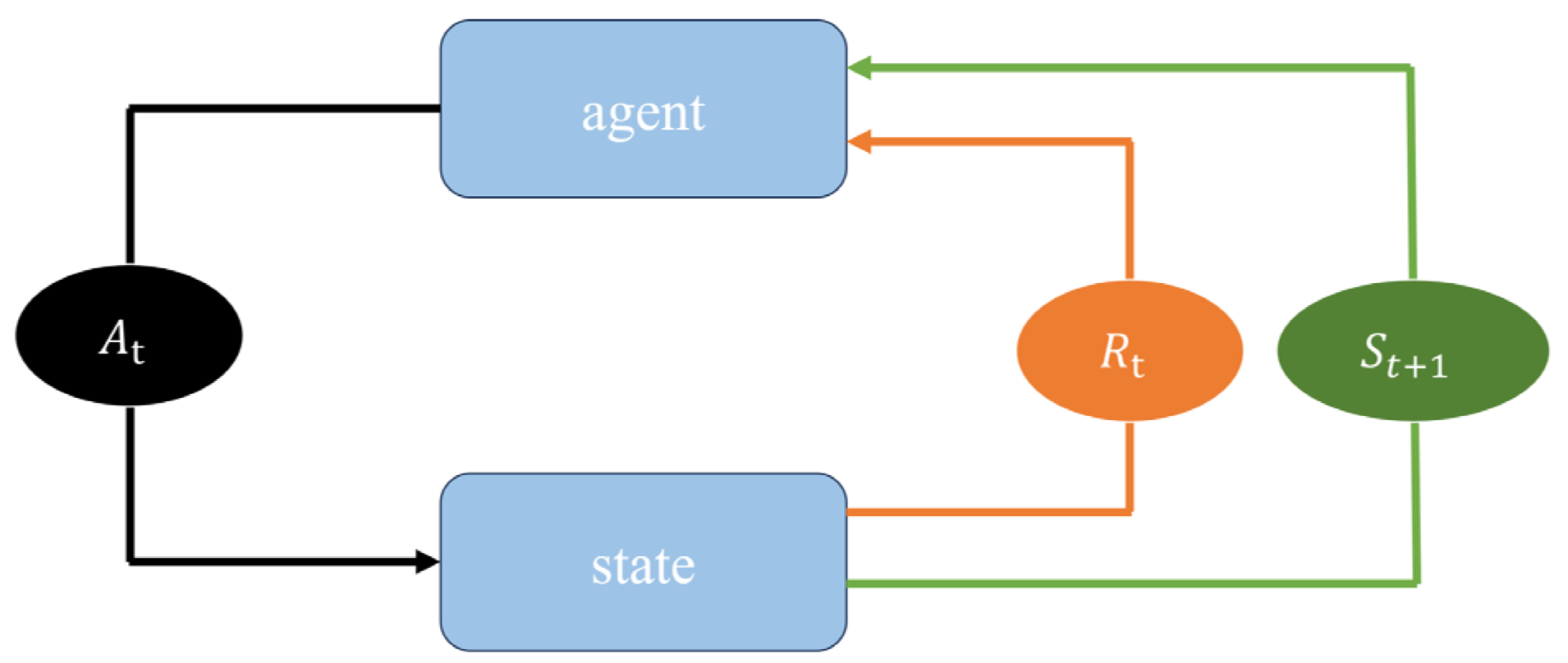
Prioritized experience replay (PER) [13] is a method employed in reinforcement learning (RL) to enhance the efficiency of experience replay [14]. Experience replay involves accumulating the agent’s experiences—comprising states, actions, rewards, and subsequent states—from its interaction with the environment and subsequently sampling these experiences randomly for training purposes during the training process.

Although algorithms such as DQN, DDQN, and Dueling DQN use uniform random sampling for experience replay, the importance of experience samples can vary significantly. Since the samples in the experience replay unit are continuously updated, if uniform random sampling is used to extract a small number of samples from the experience replay unit as model input, some highly important experience samples may not be fully utilized, thereby reducing the training efficiency of the model. In response to the problems of low data quality and low sample utilization in the experience replay mechanism of previous algorithms, and in combination with the needs of autonomous driving, this paper designs dual prioritized experience replay, DPER, and uses it as the basis for sample classification. It gives different priorities to each experience through dual-layer selection, and based on this, proposes a method based on priority experience replay, DPER.

The main contributions of this paper include the following:

This study presents a streamlined decision-making framework for autonomous vehicles, utilizing a dual-network architecture that separates ego-vehicle and environmental vehicle state processing. The design decouples action selection from evaluation through distinct parameter updating protocols, achieving precise motion control while enhancing system stability. Experimental results confirm its effectiveness in reducing Q-value overestimation and maintaining operational consistency in dynamic traffic scenarios.

The dueling network is incorporated into the double deep Q-network, merging their respective benefits and reconfiguring the original network’s output layer. This integration enhances the driverless car’s capacity to comprehend the current state and refines the precision of action value estimation. By separately assessing the state value and action advantage, the dueling network boosts the accuracy of these estimations. The double deep Q-network further reduces the overestimation bias, making the decision more robust. This structure improves the performance of traditional algorithms at multiple levels.

A new dual-priority experience replay mechanism is proposed. This paper introduces an innovative dual-priority experience replay mechanism that combines TD error priority and segmented sampling priority. The mechanism significantly improves the learning frequency and quality of key states by giving higher priority to recent experience on TD error and dynamically adjusting the state importance on segmented sampling. A comprehensive priority—that is, dual priority—is calculated based on TD error and segmented sampling. Dual-priority experience replay effectively solves the problems of low sample utilization and sparse rewards in traditional experience replay and can more effectively utilize experience replay data in unmanned highway scenarios, especially when dealing with rare but important scenarios (such as high-speed lane changes and emergency braking), which can help the DPD3QN better learn these key decisions.

The remainder of this paper is organized as follows. Section 2 introduces related work in the field of deep reinforcement learning and autonomous driving. Section 3 presents the proposed DPD3QN method, including the network structure and dual-priority experience replay mechanism. Section 4 describes the simulation environment and experimental setup. Section 5 provides the simulation results and comparative performance analysis. Finally, Section 6 concludes this study and outlines future research directions.

2. Related Works

This section outlines the approach to deep reinforcement learning. Initially, it elucidates the principles and architecture of reinforcement learning. Subsequently, it introduces the deep Q-network following Q-learning enhancements and other networks that have undergone evolutionary optimization. Ultimately, by merging the dueling Q-network with the double deep Q-network and reconfiguring the output layer of the initial network, a novel dueling double deep Q-network is formulated.

2.1. Reinforcement Learning

Reinforcement learning stands out as a highly effective approach to addressing the decision-making challenges in autonomous driving. Its objective is to identify the optimal policy that maximizes cumulative rewards. Through interaction with the environment, the intelligent agent independently explores, executes actions based on its policy to impact the environment, receives feedback in the form of rewards, and gathers data samples for learning. Through continuous learning, the agent acquires the optimal strategy. The reinforcement learning process is formulated through the Markov Decision Process (MDP) [15], with its fundamental concept illustrated in Figure 1. During each discrete time step t (where t = 1, 2, 3, …), the agent engages with the environment. At these intervals, the agent acquires a depiction of the environmental state $S_t$ ∈ S, where S denotes the collection of all potential states, and chooses an action from $A_t$ ∈ A ($S_t$), where A ($S_t$) represents the set of feasible actions in state $S_t$.

In the reinforcement learning paradigm, agents iteratively transition through state–action–reward sequences: executing action $A_t$ in state $S_t$ yields immediate reward Rt + 1 ∈ R and subsequent state St + 1. This progression forms episodic trajectories (S1, A1, S1, R1, ···, St − 1, At − 1, St, Rt − 1), terminating at St. The cumulative discounted reward Rt Equation (1) quantifies long-term performance by exponentially weighting future rewards:

$$R_t={\displaystyle \sum _{t^{\prime }=t}^T{\gamma }^{t^{\prime }-t}}{R}_{t^{\prime }-t}$$

(1)

The discount factor adjusts the weight distribution of future rewards through an exponential decay mechanism, giving higher priority to immediate rewards. The core objective of reinforcement learning is to find the optimal policy π that maximizes the cumulative discounted reward Rt. Based on this reward mechanism, the state value function $V^{\pi }$ and the action value function $Q^{\pi }$ are constructed, as shown in Equations (2) and (3). The former evaluates the long-term return of a specific state, while the latter measures the expected return of a state–action pair, as shown in Equation (3). As expressed in Equation (4), the state value function is recursively represented using the Bellman equation, and the optimal control policy π∗ is determined by maximizing the state value function, as mathematically formulated in Equation (5).

$$V^{\pi }(s_t)=E_{\pi }[R_t|s_t,\pi ]$$

(2)

$$Q^{\pi }(s_t,a_t)=E_{\pi }[R_t|s_t,a_t,\pi ]$$

(3)

$$Q^{\pi }(s_t,a_t)=E_{\pi }[r_t+\gamma \underset{a_{t+1}}{\max }{Q}^{\pi }(s_{t+1},a_{t+1})]$$

(4)

$$\pi (s_t)=\arg \underset{a_t}{\max }Q(s_t,a_t)$$

(5)

Q-learning [7] is an algorithm that employs value iteration updates to directly approximate the optimal action value function Q^∗. The Q-learning algorithm uses the update rule in Equation (6) to revise the projected value of the current action value function:

$$Q^{\ast }(s,a)\leftarrow Q(s,a)+\alpha (r+\gamma \underset{a^{\prime }}{\max }Q(s^{\prime },a^{\prime })-Q(s,a))$$

(6)

The anticipated reward for an agent when executing action $a$ in state $s$ is denoted as $Q(s,a)$. The instantaneous reward for choosing action $a$ in state $s$ is represented by $r$. The learning rate is denoted by $\alpha$, while $\underset{a^{\prime }}{\max }Q(s^{\prime },a^{\prime })$ signifies the anticipated reward for selecting alternative actions $a^{\prime }$ in the same state $s^{\prime }$. $Q(s,a)$ using Equation (6). The process will eventually converge to $Q^{\ast }(s,a)$, representing the optimal action value function [16]. This iterative method for determining the optimal action value function is known as Q-learning. To improve its generalization ability and expand its applicability, Q-learning can be integrated with deep neural networks, forming what is known as a deep Q-network.

2.2. Q-Learning Network

As the state space of the environment expands, Q-learning may face difficulties, including high memory consumption, extended search and storage durations, and challenges arising from the curse of dimensionality. To address these challenges, neural networks utilize function approximation to estimate the action value function. These networks undergo training via gradient descent to optimize a meticulously crafted loss function, thereby facilitating efficient approximation of the target values. This approach significantly reduces the storage demands associated with managing a vast number of states while enhancing the algorithm’s efficiency and scalability. Therefore, integrating deep learning architectures into reinforcement learning has become an increasingly popular trend [17].

2.2.1. Deep Q-Network

Deep Q-network (DQN) [8] overcomes the limitations of traditional Q-learning in handling large or continuous state spaces by integrating neural networks into the Q-learning framework. While conventional Q-learning relies on a Q-table to iteratively update action–state values, this tabular method becomes computationally impractical for complex environments due to storage and scalability constraints. DQN addresses this by replacing the Q-table with a parameterized neural network that approximates the action value function, where θ denotes the network weights. The target Q-value is calculated using a separate update rule, and the discrepancy between the network’s predicted Q-values and these target values is quantified through a loss function L(θ). This relationship between the estimated Q-values and the target function is formalized in Equation (7), with the true action value defined by Equation (8), enabling efficient learning through gradient-based optimization rather than explicit table maintenance.

$$L(\theta )=E[{\displaystyle \sum _{t=1}^N(}{y}_t-Q(s,a;\theta ){)}^2]$$

(7)

$$y_t=r_t+\gamma \max \underset{a^{\prime }}{\max }Q(s^{\prime },a^{\prime };{\theta }^{\prime })$$

(8)

where s′ and a′ denote the subsequent state and action after executing action a in state s. The Q-network approximates the action value function $Q(s,a;\theta )$, where θ and θ′ in Equations (7) and (8) correspond to the dual parameter sets in the DQN architecture. The primary network, parameterized by θ, determines the current policy by estimating Q-values for action selection, while the target network, with parameters θ′, computes the target Q-value. This target is derived from the immediate reward $r_t$ and discounted future reward component $\gamma \max \underset{a^{\prime }}{\max }Q(s^{\prime },a^{\prime };{\theta }^{\prime })$, reflecting the trade-off between present and anticipated returns. The interplay between these networks stabilizes training by decoupling value estimation and target generation.

2.2.2. Double Deep Q-Network

The integration of neural networks with reinforcement learning introduces the issue of overestimation. Overestimation occurs when there is a discrepancy between the estimated value function and the true value function. As a result of inaccuracies in the neural network’s evaluation model, the predicted values fail to precisely represent the true values, thereby causing consistent discrepancies. In scenarios where the action values of different actions in the same state are similar, the model might opt for a suboptimal action, preventing it from learning the optimal policy. In turn, this can reduce the overall performance of the agent.

At time t, the estimated value of the action $a$ under the selected state $s$ is represented as $Q^{estimation}\left(s,a\right)$, the target value is $Q^{target}\left(s,a\right)$, and the evaluation error caused by the function evaluation model is denoted by $Y_s^a$. Moreover, the evaluation error $Y_s^a$ is uniformly distributed in the range of [−e, e], and we can obtain Equation (9):

$$Q^{estimation}\left(s,a\right)=Q^{target}\left(s,a\right)+Y_s^a$$

(9)

DDQN [9] addresses the overestimation issue present in DQN by decoupling action selection from evaluation. First, the primary network, with parameters $\theta$, determines the action with the highest Q-value. Then, the target network, with parameters ${\theta }^{\prime }$, calculates the target value for the chosen action. The loss function $L(\theta )$ is computed based on the evaluation value, and the parameters $\theta$ of the main network are updated through backward error propagation, as outlined in Equations (10) and (11):

$$Y^{DDQN}=r_s^a+\gamma *Q(s^{\prime },\arg max Q(s^{\prime },a^{\prime },\theta ),{\theta }^{\prime })$$

(10)

$$L(\theta )=E[(Y^{DDQN}-Q(s,a,\theta ){)}^2]$$

(11)

where $\gamma$ is the discount factor and $r_s^a$ is the reward value. The loss function $L(\theta )$ is determined by the mean square error between the predicted value and the actual value.

2.2.3. Dueling Double Deep Q-Network

In reinforcement learning, estimating state values is essential, though evaluating every action in each state is not always required. The dueling double deep Q-network (D3QN) [12] extends the DDQN framework by integrating Wang’s [10] dueling architecture into both the primary and target networks. This approach decouples the Q-value estimation into two components: the state value function, which quantifies the expected return under policy π for a given state, and the action advantage function, which measures the relative benefit of selecting a specific action. By separating these elements, the D3QN enhances Q-value precision and mitigates local optima risks inherent in single-network dueling structures. The state–action value function [18], representing the anticipated reward when executing action a under policy π in state s, contrasts with the state value function that captures the policy’s overall performance in s. Their difference reflects the incremental advantage of choosing a in s, as formulated in Equation (12).

$$A^{\pi }(s,a)=Q^{\pi }(s,a)-V^{\pi }(s)$$

(12)

In the dueling network architecture, two distinct data streams are utilized: one stream generates the state value $V(s;\theta ,\beta )$, whereas the other stream outputs the action advantage value $A(s,a ;\theta ,\alpha )$ [18]. Here, θ denotes the parameters responsible for processing features in the input layer, while $\alpha$ and $\beta$ correspond to the parameters for the state value and advantage streams, respectively. The output of DDQN utilizing the dueling network structure is given by Equation (13):

$$Q(s,a ;\theta ,\alpha ,\beta )=V(s;\theta ,\beta )+A(s,a ;\theta ,\alpha )$$

(13)

Given that the network directly produces the Q-value, the state value V and action A remain unidentified. To improve identifiability, central processing of action A is employed, which enhances optimization stability while preserving performance. Here, $a^{\prime }$ represents all possible actions, and $avgA\left(s,a^{\prime };\theta ,\alpha \right)$ represents the average advantage function value across all actions. The corrected Q-value is given in Equation (14):

$$Q(s,a ;\theta ,\alpha ,\beta )=V(s;\theta ,\beta )+\left(A(s,a ;\theta ,\alpha )-avgA\left(s,a^{\prime };\theta ,\alpha \right)\right)$$

(14)

The objective function is formulated as presented in Equation (15), and the loss function utilized to adjust the network parameters is given by Equation (16):

$$y^{D3QN}=E_{(s,a,r,s^{\prime })}[r+\gamma \cdot Q_T(s^{\prime },\arg \max Q_M(s^{\prime },a^{\prime };\theta ,\alpha ,\beta );{\theta }^{\prime },\alpha ,\beta )]$$

(15)

$$L(\theta ,\alpha ,\beta )=E_{(s,a,r,s^{\prime })}[y^{D3QN}-Q_M{(s^{\prime },a^{\prime };\theta ,\alpha ,\beta )}^2]$$

(16)

where $\theta$ and ${\theta }^{\prime }$ correspond to the parameters of the primary and target networks, respectively. Additionally, $\alpha$ and $\beta$ denote the parameters of the action advantage function A and the state value function V within the dueling network framework. $Q_T$ is the action value function of the target network, while $Q_M$ is the action value function of the main network. Finally, $\arg \max Q_M(s^{\prime },a^{\prime };\theta ,\alpha ,\beta )$ represents the action $a^{\prime }$ that optimizes the Q-value of the primary network in state $s^{\prime }$.

3. DPD3QN

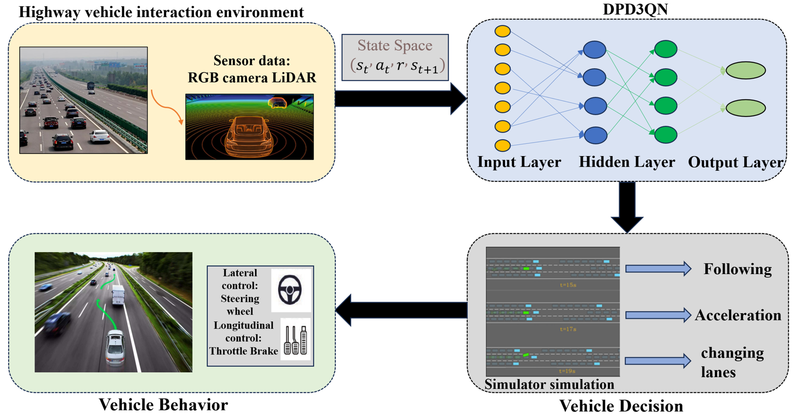
To enhance decision-making efficiency and address the limitations of uniform experience replay in the existing algorithms, this section proposes a dueling double deep Q-network (D3QN) integrated with a dual-priority experience replay mechanism (illustrated in Figure 2), which is then trained and tested in a highway scenario. Specifically, a four-lane highway simulation environment is created, and a hierarchical structure is used to control the movement of surrounding vehicles. In this structure, high-level modules determine general driving intentions—such as lane keeping, lane changing, or overtaking—while low-level modules handle specific motion control tasks, like acceleration, deceleration, and steering. This layered design improves modularity and enables more realistic and flexible traffic behavior modeling. The autonomous driving vehicle’s sensors capture real-time environmental information from the current scene and input the state data into the experience replay pool. This state is then passed to the dueling double deep Q-network. The input layer of the neural network processes the state information through intermediate layers, and the output layer translates the computed values into potential actions within the specified context. The bottom-level controller then selects and executes the optimal action based on this output.

3.1. Network Structure

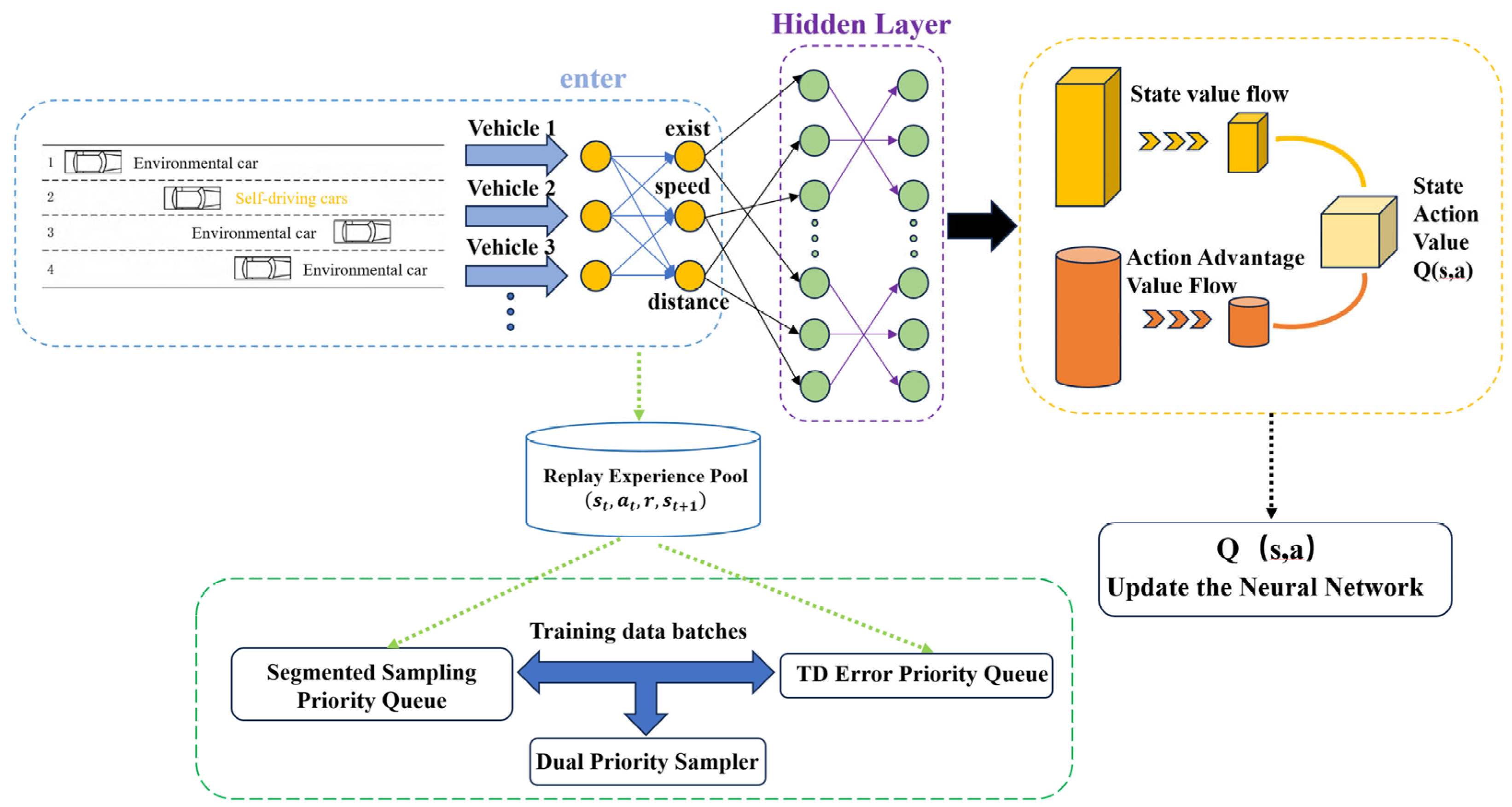
DPD3QN is a dueling double deep Q-network that integrates dual-priority experience replay; its structure is shown in Figure 3. The primary objective is to enhance the accuracy of state and action estimations via the dueling network architecture, and to improve sample efficiency and expedite the training process through a dual-priority experience replay mechanism. This approach is especially well-suited for sequential decision-making tasks, such as autonomous driving.

Figure 2 shows a reinforcement learning architecture of a dueling double deep Q-network based on dual-priority experience replay, aimed at enhancing learning efficiency and decision-making precision. The entire procedure can be segmented into the subsequent components:

In the input module, this paper employs the state information from multiple vehicles, encompassing attributes like vehicle presence, speed, and distance. Each vehicle’s characteristics are vectorized to create a state representation, which is then fed into the neural network’s hidden layer.

The experience replay buffer stores the experience tuples $\left(s_t,a_t,r,s_{t+1}\right)$ generated by the agent as it interacts with the environment. Utilizing this replay buffer efficiently disrupts the temporal correlation among data samples, enhances sample utilization, and mitigates overfitting. This module ensures the stability of the training process by storing past experience data.

Priority sampling method: To enhance learning efficiency even more, the replay pool adopts a dual-priority sampling mechanism. First, the TD error is used to measure the importance of the sample, and the empirical samples are sorted through the priority queue, giving priority to samples with larger errors for training. At the same time, a segmented sampling mechanism is used to extract samples from different priority queues to ensure the diversity of the training samples. This method can accelerate model convergence and improve sample utilization.

Neural network structure: As shown in Figure 3, the hidden layer of the network is responsible for extracting high-dimensional features of the input state. Following the hidden layer, the network bifurcates into two streams: one for state value and another for action advantage. The state value stream V assesses the worth of the current state $s_t$, whereas the action advantage stream A evaluates the relative benefits of each action $a_t$ within this state. This design is based on the dueling network structure, which enables the model to better distinguish action choices under different states, thereby improving decision quality. Ultimately, the two streams are combined to produce the Q-value, denoted as $Q(s,a)$, which the agent utilizes to determine the optimal action.

Q-network update: The network parameters are adjusted by computing the discrepancy between the predicted Q-value and the target Q-value. Specifically, the TD error is determined using the Bellman equation to inform the modification of the network weights. This procedure is iterated numerous times, enabling the model to progressively converge and allowing the agent to learn the optimal strategy in a dynamic environment.

3.2. Priority Experience Replay

3.2.1. Prioritization Based on TD Error

Experience replay was first proposed by Schual [13] and applied to DQN. This method determines the importance of each sample based on temporal difference (TD). Samples with higher priority are more likely to be selected for training. This priority can be calculated based on TD error. TD error signifies the discrepancy between the anticipated value and the actual reward value. Its calculation formula is shown in Equation (17):

$$\delta =|r+\gamma {\max }_{a^{\prime }}Q(s^{\prime },a^{\prime };{\theta }^{-})-Q(s,a;\theta )|$$

(17)

where $r$ is the immediate reward, $\gamma$ is the discount factor, $Q(s^{\prime },a^{\prime };{\theta }^{-})$ is the target network output, and $Q(s,a;\theta )$ is the output of the current network. The sum of the two TD errors generated by the dual networks and the immediate reward is used as the basis for dividing the importance. The empirical priority value $p(i)$ can be defined as Equation (18):

$$p(i)={({\delta }_i+ϵ)}^a$$

(18)

where $ϵ$ is a small constant that prevents the priority of the data from being zero. The hyperparameter $a$ determines the degree of influence of the TD error ${\delta }_i$ on the sample selection and controls the sensitivity to the error during sampling. Experience with high priority will have a greater chance of being sampled. The larger the TD error, the higher the priority. In the early training process, the TD error may be inaccurate. In light of the aforementioned factors, it is necessary to decrease the priority weight when selecting training data during the initial phase of the training process. At the same time, in order to ensure that even samples with extremely low priority can be selected, we add a bias to the priority compared to the traditional priority approximate distribution $b$ [13]. In our experiments, the value of the bias term b is set to 0.01, which helps avoid zero probability and ensures sufficient sample diversity. The approximate distribution of an experience sample being taken is improved to Equation (19):

$$P(i)={\displaystyle \frac{p_i^{\alpha }}{{\displaystyle \sum _{i=1}^k{p}_i^{\alpha }}}}+b$$

(19)

The sampling probability for the i-th experience is determined by the parameter α through the priority mechanism, where α serves as a balancing coefficient between prioritized and uniform sampling. Specifically, α ∈ [0,1] controls the degree of priority emphasis in the probability distribution $p_i$, which represents the priority of the i-th transition—typically defined based on the magnitude of its temporal difference (TD) error, such as p_i = ∣δi∣ + ε, where δi is the TD error and ε is a small positive constant to ensure a non-zero probability. When α approaches 1, the selection process predominantly follows the temporal difference error ranking, while values near 0 implement conventional random sampling. To mitigate potential overfitting caused by repeatedly selecting similar high-priority transitions, the algorithm incorporates a baseline probability adjustment through hyperparameter ε. This safeguard prevents the sampling distribution from becoming excessively skewed toward historically high-priority experiences, thereby maintaining the diversity of training samples and improving generalization capability. The parameter α essentially operates as a continuous interpolation regulator between two sampling paradigms: complete priority dominance (α = 1) and pure stochastic selection (α = 0).

Since the agent tends to replay experiences with higher TD errors more frequently, it will undoubtedly change the frequency of state visits. This change may cause the training process of the neural network to oscillate or even diverge [19]. To solve this problem, this paper uses importance sampling weights, as shown in Equation (20), when calculating weight changes:

$$w(i)={\left({\displaystyle \frac{1}{N}}\cdot {\displaystyle \frac{1}{P(i)}}\right)}^{\beta }$$

(20)

where β represents the parameter governing bias correction in prioritized sampling, and N denotes the total capacity of the experience replay buffer. During agent–environment interactions, β is progressively annealed from its initial value to 1. To counteract sampling bias, the loss function integrates importance sampling weights (β-adjusted), and gradients are optimized to minimize distortions caused by prioritized experience selection.

3.2.2. Prioritization Based on Segment Sampling

Based on the TD error-based priority, this paper further introduces Stochastic Prioritization [20], which is inspired by the mini-batch gradient descent [21] in the Deep Deterministic Policy Gradient (DDPG) deep reinforcement learning algorithm. By dividing the data into multiple small batches, segmented sampling can achieve efficient learning and stability in complex environments. This method effectively improves the utilization of data in the experience pool and enables samples of different priorities to be effectively extracted, thereby accelerating the convergence of the model and avoiding overfitting or insufficient data utilization in a high-dimensional continuous action space.

The specific steps of segmented sampling priority are as follows: First, the features are divided into two main segments: the position segment, including the distance to the preceding vehicle or the relative lane position, and the speed segment, covering the vehicle speed range. The data of the entire experience replay buffer are divided into different segments according to these features. Then, the segment to which each sample $i$ belongs is defined as $s(i)$ and a weight is set for each segment.

For the position segment, the priority can be set according to the scarcity and importance of the preceding vehicle distance. In certain specific distance ranges (such as close or far distances), the number of samples is small, and a higher weight should be given to ensure that the scenes of these critical distances are fully paid attention to. This diversity can be captured by measuring the standard deviation of samples within a position segment. The specific weight setting can be expressed as Equation (21):

$$w_{\mathrm{position}}(s(i))=g(n(s(i)),{\sigma }_{\mathrm{pos}}(s(i)))$$

(21)

where $w_{\mathrm{position}}(s(i))$ is the weight of the position segment $s(i)$, $n(s(i))$ is the number of samples in segment $s(i)$, and ${\sigma }_{\mathrm{pos}}(s(i))$ is the standard deviation of the distance to the preceding vehicle in segment $s(i)$. A higher standard deviation indicates that the scene changes more within the segment, so more attention is needed. The function g(⋅) is a mapping function that combines the number of samples and the variability in position to determine the importance of the position segment. It typically increases with larger ${\sigma }_{\mathrm{pos}}$ and may decrease or normalize based on $n(s(i))$, thereby balancing between data abundance and scene dynamics.

Meanwhile, the weight of the speed segment can be expressed as Equation (22):

$$w_{\mathrm{speed}}(s(i))=h(n(s(i)),{\sigma }_{\mathrm{speed}}(s(i)))$$

(22)

where $w_{\mathrm{speed}}(s(i))$ is the weight of speed segment $s(i)$ and ${\sigma }_{\mathrm{speed}}(s(i))$ variability is determined by the standard deviation of the speed measurements within segment $s(i)$. In addition, emergency situations on highways (such as emergency braking or avoidance) are more important than ordinary driving scenarios, so these segments are artificially given higher weights. The function h(⋅) is similar to g(⋅), serving as a mapping from the speed variability and the segment size to a scalar importance value, emphasizing segments with abrupt speed changes or rare events.

The weight of ordinary driving can be set to $w_{\mathrm{normal}}=1$, the weight of emergency braking to $w_{\mathrm{emergency}}=3$, the weight of lane change operation to $w_{\mathrm{lane} \mathrm{change}}=3$, and the weight of close driving to $w_{\mathrm{close}}=2$. By setting priorities in this way, we ensure that important scenarios are fully paid attention to during training, thereby improving the overall performance and adaptability of the model.

3.2.3. Dual Priority Calculation

Based on the TD error priority and the segment sampling priority, a comprehensive priority is calculated—that is, a dual priority. For each sample $i$, its comprehensive priority $P_i$ can be calculated by combining the TD error priority and the segment weight. The comprehensive priority can be expressed as Equation (23):

$$P(i)=\delta \cdot P_{\mathrm{TD}}(i)+\eta \cdot (w_{\mathrm{position}}(s(i))+w_{\mathrm{speed}}(s(i)))$$

(23)

where $P_{\mathrm{TD}}(i)$ is the TD error priority of sample $i$, $w_{\mathrm{position}}(s(i)$ and $w_{\mathrm{speed}}(s(i))$ are the weights of the position information and velocity information segments to which the sample belongs, respectively, and $\delta$ and $\eta$ are hyperparameters that control the influence of their respective weights. Based on the dual priority $P(i)$, we then perform weighted sampling to ensure that the model can pay more attention to important samples. Specifically, the sampling probability of sample $i$ can be determined by the following Equation (24):

$$P(s(i)=k)={\displaystyle \frac{P_i}{{\displaystyle \sum _j{P}_j}}}$$

(24)

where the numerator $P_i$ is the comprehensive priority of sample $i$ and the denominator ${\displaystyle \sum _j{P}_j}$ is the sum of the comprehensive priorities of all samples. Thus, the likelihood of sample $i$ being selected is proportional to its overall priority.

It is important to note that α + β is not strictly constrained to equal 1. This design provides greater flexibility, allowing the relative importance of TD error and segment-based priority to be dynamically adjusted during different training stages. For example, in the early stages of training, when the model has not yet learned an effective policy and the TD error tends to fluctuate significantly, a higher α can be used to emphasize learning from large-value errors and accelerate policy correction. In contrast, during the later stages—when the policy becomes more stable—β can be increased to direct the model’s attention to rare but critical driving scenarios, such as high-speed lane changes or emergency braking. This helps improve the generalization and real-world adaptability of the learned policy.

Moreover, since both the TD error and the segment weights are not inherently bounded, the combined priority value $P_i$ may theoretically exceed 1. To address this, we apply a normalization process during the sampling stage by dividing each priority by the total priority sum ${\displaystyle \sum _j{P}_j}$, resulting in the normalized sampling probability. This ensures that each sample is selected according to its relative importance, regardless of the absolute value. At the same time, it prevents high-priority samples from dominating the training process, thereby reducing the risk of overfitting or biased learning.

This approach not only maintains training efficiency but also enhances the model’s ability to learn from diverse types of scenarios with increased robustness. By adjusting α and β, researchers and developers can fine-tune the training process based on specific task demands and environmental complexities. In future versions, we also plan to include a schematic illustration and a numerical example to further improve the transparency and interpretability of the dual-priority formula. A simple calculation example is added in this section to enhance the understanding of the formula, as shown in

Table 1. Example calculation.

Example: Dual-Priority Calculation
Consider a sample with the following attributes:
TD error: $p_i^{TD}$ = 0.75;
Position segment weight: $w_i^{pos}$ = 0.20;
Velocity segment weight: $w_i^{vel}$ = 0.15;
Given hyperparameters: α = 0.6, β = 0.4.
Then, the comprehensive priority is as follows:
$P_i$ = 0.6 × 0.75 + 0.4 × (0.20 + 0.15) = 0.45 + 0.14 = 0.59.
If the sum of priorities in the current batch is ${\sum }_j{P}_j$ = 5.9,
then, the normalized sampling probability is as follows:
$P_i^{sample}$ = 5.9/0.59 = 0.10.

.

This example clearly demonstrates how to combine the TD error and semantic segment weights to compute the comprehensive priority and normalize it into a sampling probability.

This priority sampling method, which combines TD error and segment weights, namely, dual-priority sampling, can more effectively utilize experience playback data in unmanned highway scenarios, especially when dealing with rare but important scenarios (such as high-speed lane changes and emergency braking), which can help the DPD3QN better learn these key decisions and ensure the stability and convergence speed of the training process.

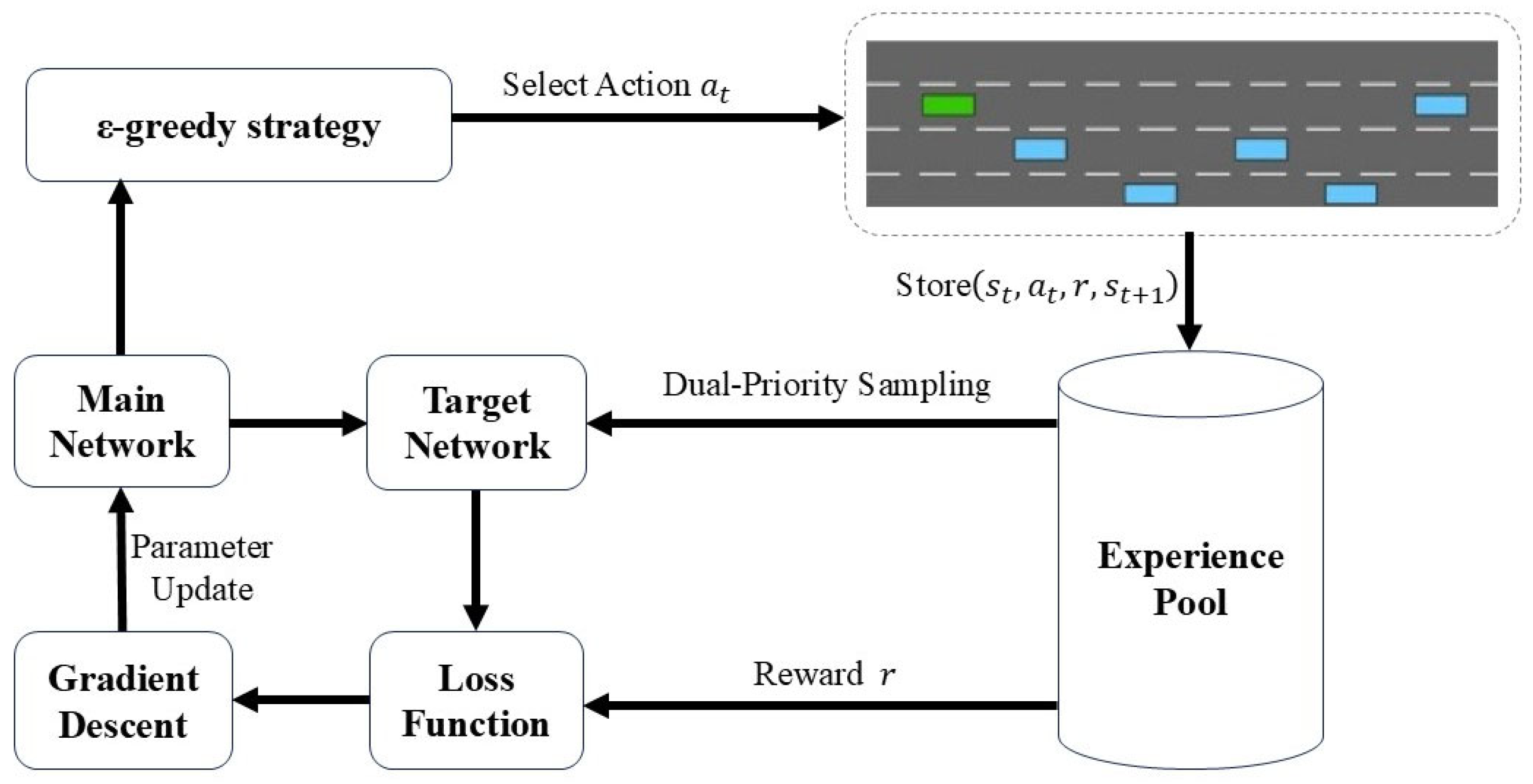
Based on the integration of the dueling network and the DDQN structure, this paper uses dual-priority experience replay to update the experience pool and update the parameters of the neural network, as shown in Figure 4.

During the autonomous driving process, the system first selects the current action $a_t$ from the main network using the ϵ-greedy strategy [22]. This strategy strikes a balance between exploration (selecting random actions) and exploitation (selecting the best action), exploring new strategies by randomly selecting actions with a small probability and selecting the best action evaluated by the main network at other times. Once the action has been chosen, the system executes $a_t$ and then engages with the simulated driving scenario and interacts within it to generate the next state $s_{t+1}$ and reward value $r$. This information (current state $s_t$, action $a_t$, reward $r$, and next state $s_{t+1}$) is stored in the experience pool. The experience pool is used to record multiple historical data for experience playback during training. The system extracts samples from the experience pool and calculates the TD error of these samples through the target network to calculate the loss function. The TD error reflects the gap between the prediction and the actual reward and is the core optimization target of training. The main network’s parameters are refined via the gradient descent method, employing the backpropagation algorithm to reduce the loss function, thereby enhancing the network’s predictive performance progressively. To ensure stability, the target network’s parameters are not adjusted in real time but are periodically updated to match those of the main network. This structure helps prevent the target value from fluctuating too much, thereby improving the stability of training. The system repeats the above process continuously, gradually updating the network parameters and improving the strategy, thereby achieving more intelligent decision-making in unmanned driving scenarios.

The ϵ-greedy [22] strategy facilitates the equilibrium between exploration and exploitation throughout the reinforcement learning training phase, ensuring that the agent both investigates novel states and actions and leverages accumulated knowledge to choose the most advantageous action. The implementation proceeds as follows: at each time step, an action is chosen randomly with probability ϵ, while the action deemed optimal by the current Q-network is selected with probability 1 − ϵ. Following a set number of training iterations, the approach is assessed, and adjustments are made to the exploration strategy or algorithm parameters in accordance with the evaluation outcomes. The exploration process usually gradually reduces the value of ϵ so that the agent explores more in the early stage of training and exploits more in the later stage of training. The algorithm is shown in Equation (25):

$${ϵ}_t=\max ({ϵ}_{\min },{ϵ}_{\mathrm{decay}}\cdot {ϵ}_{t-1})$$

(25)

where ${ϵ}_t$ is the exploration rate at time step t, ${ϵ}_{\min }$ is the minimum value of the exploration rate, ${ϵ}_{\mathrm{decay}}$ is the decay factor of the exploration rate, and ${ϵ}_{t-1}$ is the exploration rate at time step t − 1. Equation (25) indicates that at each time step t, the exploration rate ϵ will decay with a fixed decay factor ${ϵ}_{\mathrm{decay}}$ but will not fall below the preset minimum value ${ϵ}_{\min }$.

4. Experiment and Its Simulation Environment

This section analyzes the operational framework for multi-lane highway environments and the hierarchical control architecture regulating vehicle motion across lateral (steering) and longitudinal (acceleration/braking) axes. At the actuation level, proportional-derivative (PD) controllers enable accurate trajectory tracking and speed adjustment. The experimental setup leverages the Highway-env platform [23], a simulation tool integrated with OpenAI Gym, to model a four-lane highway environment. This platform emulates real-world traffic dynamics, facilitating structured testing of autonomous driving algorithms under diverse yet controlled highway scenarios. Parameters such as traffic flow variability and control precision are systematically configured to validate strategy robustness.

4.1. Highway Environment

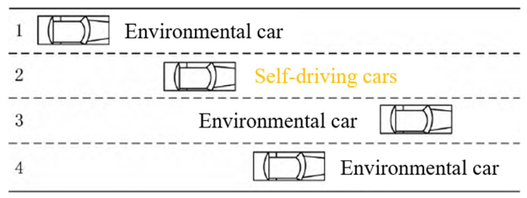
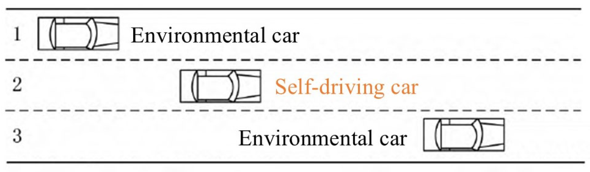
This section analyzes operational decision-making frameworks for autonomous navigation, focusing on achieving specific navigational goals through strategic action sequences. Within the controlled expressway environment, these core operational modalities manifest as propulsion adjustments (speed modulation), lateral maneuvers (lane transitions), and velocity maintenance. The simulation environment is shown in Figure 5. The experimental setup adopts a dual-agent system, consisting of a self-driving vehicle and several environment vehicles that mimic human driving behavior. All vehicles operate based on the previously mentioned motion model and environmental configuration, aiming to study the interactive dynamics under standardized highway conditions. The investigation employs a parametric analysis approach, quantifying control responses through measurable kinematic variables including relative velocities, inter-vehicle spacing, and trajectory deviation metrics.

To enhance the realism and unpredictability of the driving scenario, this paper randomly determines the initial speed and starting position of the environmental vehicle. This practice helps to simulate the actual driving situation more realistically and enhance the adaptability of the autonomous vehicle in complex environments. In addition, in order to better imitate human driving habits, we set the autonomous vehicle to drive as far to the right as possible when there is no need to overtake. These settings are designed to improve the realism of the driving scene.

Prior to initiating the driving task, 60 environmental vehicles are randomly positioned on a four-lane highway ahead of the autonomous vehicle. Each simulation cycle, termed a round, commences with the autonomous vehicle’s activation and concludes upon either its successful completion of the journey within a 30 s timeframe or collision with surrounding vehicles. Vehicle configurations follow standardized parameters: all units measure 5 m in length and 2 m in width. Environmental vehicles are assigned randomized initial speeds between 20 and 30 m·s⁻¹, while the autonomous vehicle starts at 25 m·s⁻¹. Operating at a 10 Hz simulation frequency [24], rounds are automatically reset upon meeting termination criteria, ensuring iterative scenario testing under controlled temporal constraints. For the specific settings of vehicle parameters, see

Table 2. Vehicle parameter settings.

Parameter	Numeric
Number of lanes	4
Vehicle length/m	5
Vehicle width/m	2
Initial speed of environmental vehicle/(m·s−1)	20–30
Initial speed of autonomous vehicle/(m·s−1)	25
Simulation frequency/hz	10
Round time limit/s	30

.

4.2. Vehicle Behavior Control

In this research, the environmental vehicles are governed by the intelligent driving model (IDM) [25] and the overall braking model (MOBIL) [26]. In addition, this paper uses deep reinforcement learning methods to control the behavior of the autonomous driving vehicle.

The IDM is a common microscopic model used to control the longitudinal behavior of the vehicle. The model accomplishes vehicle following and collision prevention by assessing the spacing and relative velocity between vehicles. Generally, the longitudinal acceleration in the IDM can be described by Equations (26) and (27).

$$\stackrel{-}{v}=a_{\max }\left[1-{\left({\displaystyle \frac{{\nu }_c}{{\nu }_t}}\right)}^{\delta }-{\left({\displaystyle \frac{d^{*}}{d_c}}\right)}^2\right]$$

(26)

$$d^{*}=d_{\min }+T{\nu }_c+{\displaystyle \frac{{\nu }_c\Delta {\nu }_c}{2\sqrt{a_{\max }{a}_{\min }}}}$$

(27)

The IDM defines vehicle dynamics through the following critical variables: $\stackrel{-}{v}$ denotes the current velocity of the subject vehicle, while $a_{\max }$ specifies the peak acceleration capability. The parameter $d^{*}$ quantifies the gap distance to the leading vehicle, and ${\nu }_t$ indicates the desired cruising speed. A nonlinear velocity regulation coefficient, denoted as δ, governs speed adaptation responsiveness. Safety constraints are enforced via T, a temporal safety buffer defining the minimum acceptable time-to-collision threshold, and $\Delta {\nu }_c$ captures the relative velocity differential between vehicles. The model further incorporates $d_{\min }$ as the mandatory minimum inter-vehicle spacing and $a_{\min }$ as the maximum emergency braking capacity. The parameters are configured as follows: the maximum acceleration is 6 m·s⁻², the speed index parameter is 5, the required time interval T is 1.5 s, the maximum deceleration is −5 m·s⁻², and the minimum distance is 12 m.

By contrast, the MOBIL model governs the vehicle’s decision to change lanes laterally. This model takes into account the safety and incentive criteria between vehicles to ensure that when changing lanes, the new following vehicle does not cause a collision risk due to sudden deceleration. Within the mobility-oriented lane-changing decision framework, the kinematic response of the target lane’s following vehicle is quantitatively evaluated through Equation (28), where the critical parameter $b_{safe}$ characterizes the maximum emergency braking intensity imposed on the following vehicle during lane changes. To ensure operational safety, the system employs a dual-layer constraint mechanism: Equation (29) rigorously defines the acceleration threshold $a_{th}$ for safety criteria, which holistically integrates vehicular dynamic constraints and traffic flow stability requirements. This threshold enables optimal decision-making by dynamically balancing traffic throughput efficiency and risk mitigation requirements.

$${\tilde{a}}_n\ge -b_{safe}$$

(28)

$$\underset{egovehicle}{\underbrace{{\tilde{a}}_e-a_e}}+p\cdot \left(\underset{newfollower}{\underbrace{a_n-a_n}}+\underset{oldfollower}{\underbrace{a_0-a_0}}\right)\ge a_{th}$$

(29)

The coordinated velocity optimization mechanism, governed by Equations (28) and (29), ensures systematic speed improvements for the ego vehicle, its immediate follower, and downstream traffic participants in both original and target lanes. Within the MOBIL decision framework, critical operational parameters are calibrated as follows: the social compliance coefficient (p = 2 × 10⁻⁴) modulates cooperative interaction intensity between vehicles, while the safety-critical deceleration boundary ($b_{safe}$ = 2.5 m·s⁻²) establishes emergency braking limits to prevent collision risks. Concurrently, the maneuver benefit threshold ($a_{th}$ = 0.25 m·s⁻²) enforces a minimum acceleration advantage requirement for lane-change authorization.

4.3. Vehicle Motion Control

Upon completion of the vehicle motion decision process, the lower control layer primarily governs the vehicle’s longitudinal and lateral movements via proportional and proportional-differential controllers [27]. The longitudinal motion is managed by the proportional controller with acceleration, which is mathematically defined as Equation (30), where $\dot{\nu }$ denotes the vehicle’s present longitudinal acceleration, $\nu$ signifies the vehicle’s current speed, ${\nu }_r$ is the set speed, and $K_p$ represents the controller’s proportional gain:

$$\dot{\nu }=K_p\left({\nu }_r-\nu \right)$$

(30)

In the context of lateral movement, the proportional-derivative controller governs the vehicle’s lateral position. Its expression is characterized as presented in Equations (31) and (32), where $v_{lat,r}$ is the lateral velocity command, $K_{p,lat}$ is the position gain, and ${\Delta }_{lat}$ is the lateral position of the vehicle relative to the centerline of the lane:

$$v_{lat,r}=-K_{p,lat}{\Delta }_{lat}$$

(31)

$$\Delta {\psi }_r=\arcsin ({\displaystyle \frac{{\nu }_{lat,r}}{\nu }})$$

(32)

In this scenario, all environmental vehicles realize their behavior and motion management through the above two-layer control framework.

4.4. Experimental Parameter Settings

This experiment assumes that the autonomous vehicle can sense the 10 nearest environmental vehicles within 250 m before and after its position and accurately obtain the distance and speed information of these vehicles relative to the autonomous vehicle, which is used as an important part of the environmental state. The definition of its environmental state is Equations (33) and (34):

$$\Delta s_{\mathrm{t}}=\mid s_t-s_t^{enviroment}|$$

(33)

$$\Delta v_t=\mid v_t-{\nu }_t^{environment}|$$

(34)

The policy update frequency is set to 1 Hz. The road in the experiment is divided into four lanes, and the surrounding environment contains 50 other vehicles. The discount factor γ is set to 0.95, indicating that future rewards decay exponentially, and the learning rate α is 0.0002, which controls the step size of the state change in each update. Both the value network and the advantage network feature layers with 64 neurons each, defining the network’s width. The training process lasts for 5000 rounds, during which ϵ is gradually reduced from 1 to 0.05. As the training progresses, exploration is reduced, and action selection is based more on the currently learned strategy.

The reward function $r_t$ consists of the optimal control goal, which is to avoid collisions during driving and drive in the right lane as fast as possible. To achieve this control goal, the round reward function is set as shown in Equation (35):

$$r_t=1-collision+0.4\times r_{\nu }+0.1\times (L-1)$$

(35)

where $collision$ ∈ [0,1] (0 means no collision, 1 means collision), $r_v$ is the speed reward, $r_v$ ∈ [24,30], and L is the lane position.

5. Simulation Results Analysis

5.1. Training Analysis

This subsection conducts a comparative analysis of three representative deep reinforcement learning algorithms—Deep Q-Network (DQN) [8], double deep Q-network (DDQN) [9], and the proposed dual-priority delayed deep double Q-network (DPD3QN)—through a multi-dimensional performance evaluation framework. Under identical initialization parameters, the experimental design specifically examines four critical performance dimensions: (1) policy convergence characteristics and training stability, (2) cumulative reward acquisition efficiency, (3) state space exploration capability, and (4) overestimation error suppression effectiveness.

Figure 6 illustrates the round rewards achieved by the three algorithms. A greater reward signifies that the self-driving vehicle is navigating the highway with increased efficiency. As shown in Figure 6, the learning speed of DPD3QN is noticeably faster than the other two methods. By approximately the 1200th iteration, the mean reward of DPD3QN exceeds that of the other two approaches and sustains this lead until training concludes. By the conclusion of 5000 rounds, the average rewards for DQN, DDQN, and DPD3QN are 12.48, 12.92, and 13.35, respectively. This improvement can be attributed to the dueling network architecture in DPD3QN, which accurately assesses the value of the selected action at each step, enabling the autonomous vehicle to identify better decision-making strategies more efficiently.

Figure 7 illustrates the driving distance for each round throughout the training phase for the three decision-making approaches. The driving distance is mainly affected by collision conditions and vehicle speed. A greater driving range allows autonomous vehicles to maintain high speeds for extended durations without incidents. During the training process, the driving distance of the autonomous vehicle will vary due to the unpredictable initial speeds and positions of nearby vehicles. In the first 800 rounds, the driving distances of the three decision-making methods are similar, and the difference is not obvious. After 800 rounds, the driving distance achieved by the DPD3QN decision-making approach progressively exceeded that of the other two methods, and this pattern persisted until the conclusion of training. At the end of 5000 rounds, the driving distances of DQN, DDQN, and DPD3QN were 551 m, 622 m, and 694 m, respectively. Although the performance of the three methods in the exploration phase is similar, DPD3QN’s dual-priority experience replay can identify and utilize key experiences faster, thereby accelerating the learning process and making better choices. This mechanism significantly improves the response ability of autonomous vehicles to environmental changes and verifies the superiority of this method.

Figure 8 evaluates the safety performance of the three algorithms through episode duration analysis, where longer operational periods reflect enhanced driving stability. DPD3QN recorded the highest average step count at 27.34 per episode, surpassing DDQN (24.66) and DQN (22.79). Notably, episodes exceeding 25 steps signify robust long-distance safety, with DPD3QN achieving 2945 instances beyond 27 steps—substantially higher than DDQN (1709) and DQN (474). This demonstrates DPD3QN’s superior collision avoidance capability, highlighting its safety advantages over baseline methods. Given the critical role of operational reliability in autonomous systems, the DPD3QN-based decision model exhibits stronger practical viability for real-world deployment.

5.2. Adaptability Test

5.2.1. Test Scenario I

Following highway environment training, two enhanced evaluation scenarios were developed to test the autonomous vehicle’s adaptive performance. The first test configuration maintained the training phase’s surrounding vehicle count and core parameters but reduced the highway to three lanes and extended trial iterations to 1000. The simulation environment is shown in Figure 9. Pretrained neural network models were deployed without adjustments to evaluate generalization in altered conditions. The performance metrics for this modified scenario are detailed in the following analysis.

Figure 10 illustrates the success rates of the three models in the testing scenario. As the number of test rounds increases, the selection of control actions enables the autonomous vehicle to continuously reach the specified time limit, so the success rate shows an upward trend. At the end of the test round, the success rate of the DPD3QN model reached 72.6%. This shows that DPD3QN can effectively quantify the potential value of the current control action and update the target network parameters, thereby improving the control performance. The specific test results are shown in

Table 3. Test results I.

Algorithm Model	Success Rate (%)	Average Reward	Average Speed (m·s−1)
DPD3QN	70.6	13.78	27.78
DDQN	58.8	12.56	26.54
DQN	44.8	11.19	26.31

. In two driving scenarios depicted in Figure 10, the autonomous vehicle showed different results.

Figure 11a shows a common driving scenario in real life. Three environmental vehicles occupy three lanes, which makes it impossible for the autonomous vehicle behind to drive at a higher speed. The autonomous vehicle has to wait, make a decision to accelerate and change lanes two seconds after following the environmental vehicle, and successfully completes the lane change. Figure 11b shows another lane change result. Due to the autonomous vehicle’s failure to accurately assess the speed of the adjacent vehicle in a timely manner while following the preceding vehicle, it could not change lanes in time and collided with the other vehicles.

In Figure 11, the green square represents the self-driving vehicle, and the blue square represents the environment vehicle. When the self-driving vehicle collides with the environment vehicle, both vehicles are shown in red in the simulation environment.

5.2.2. Test Scenario II

Based on test scenario I, a more complex driving scenario was constructed, with the six environmental vehicles within the 200 m range before and after the autonomous driving vehicle being sensed increased to 10. At the same time, the policy update frequency was set to 0.5 Hz so that the model could adapt to environmental changes more slowly. Other parameters remained the same as scenario I.

Figure 12 shows the collision of the three decision algorithms during the test, where collision is defined as two values: collision = 0 means that the autonomous vehicle has not collided with other vehicles; collision = 1 means that the autonomous vehicle has collided with other vehicles. The results show that DPD3QN and DDQN successfully avoided collisions after 733 and 827 rounds, respectively. This shows that the DPD3QN method performs particularly well when dealing with complex scenarios. This advantage is attributed to the introduction of dual-priority experience replay, which helps autonomous vehicles identify and utilize key experiences more quickly, thereby accelerating the learning process and making better choices. In addition, the existence of the dueling network structure enables the algorithm to take into account the state value when updating the action value, thereby more accurately obtaining the Q-value corresponding to each action. The specific test results are shown in

Table 4. Test results II.

Algorithm Model	Success Rate (%)	Average Reward	Average Speed (m·s−1)
DPD3QN	65.7	12.65	26.95
DDQN	56.9	11.01	26.11
DQN	43.5	9.79	25.89

:

This result is due to the increase in the complexity of the test scenarios, which leads to a decrease in the success rate and average speed of autonomous vehicles in the decision-making process. At the same time, the number of collisions increases, which, in turn, leads to a decrease in the reward obtained per round and, ultimately, a decrease in the average reward.

As demonstrated in Table 4, the DPD3QN algorithm achieves a success rate surpassing DDQN and DQN by 8.8% and 22.2%, respectively, in scenario II testing. It also exhibits superior performance in both average reward and speed metrics. Upon test completion, DPD3QN yielded an average reward of 12.65 and maintained a speed of 26.95 m·s⁻¹, outperforming DDQN (11.01 reward, 26.11 m·s⁻¹) and DQN (9.75 reward, 25.89 m·s⁻¹). These results validate the enhanced learning efficiency, decision-making precision, and operational stability of the proposed method compared to conventional reinforcement learning frameworks.

6. Conclusions

This study employs deep reinforcement learning techniques to examine the decision-making processes of autonomous vehicles in highway settings and introduces a dueling double deep Q-network utilizing dual-priority experience replay (DPD3QN). Through theoretical comparison with the traditional DQN and DDQN methods, it is proved that the proposed adaptive optimal autonomous driving behavior decision-making method has significant advantages in decision-making performance and applicability.

(1) An efficient and safe decision network framework is constructed. By combining the dueling network with the double deep Q-network, this paper reconstructs the output layer of the original network, enhances the autonomous driving system’s ability to understand the current state, and improves the accuracy of the estimation of action value.

(2) A dual-priority experience playback mechanism is introduced, allowing the system to identify and utilize key experiences faster. When updating network parameters, the weight distribution of old and new experiences can be better balanced, thereby significantly improving the update efficiency and convergence speed of the network.

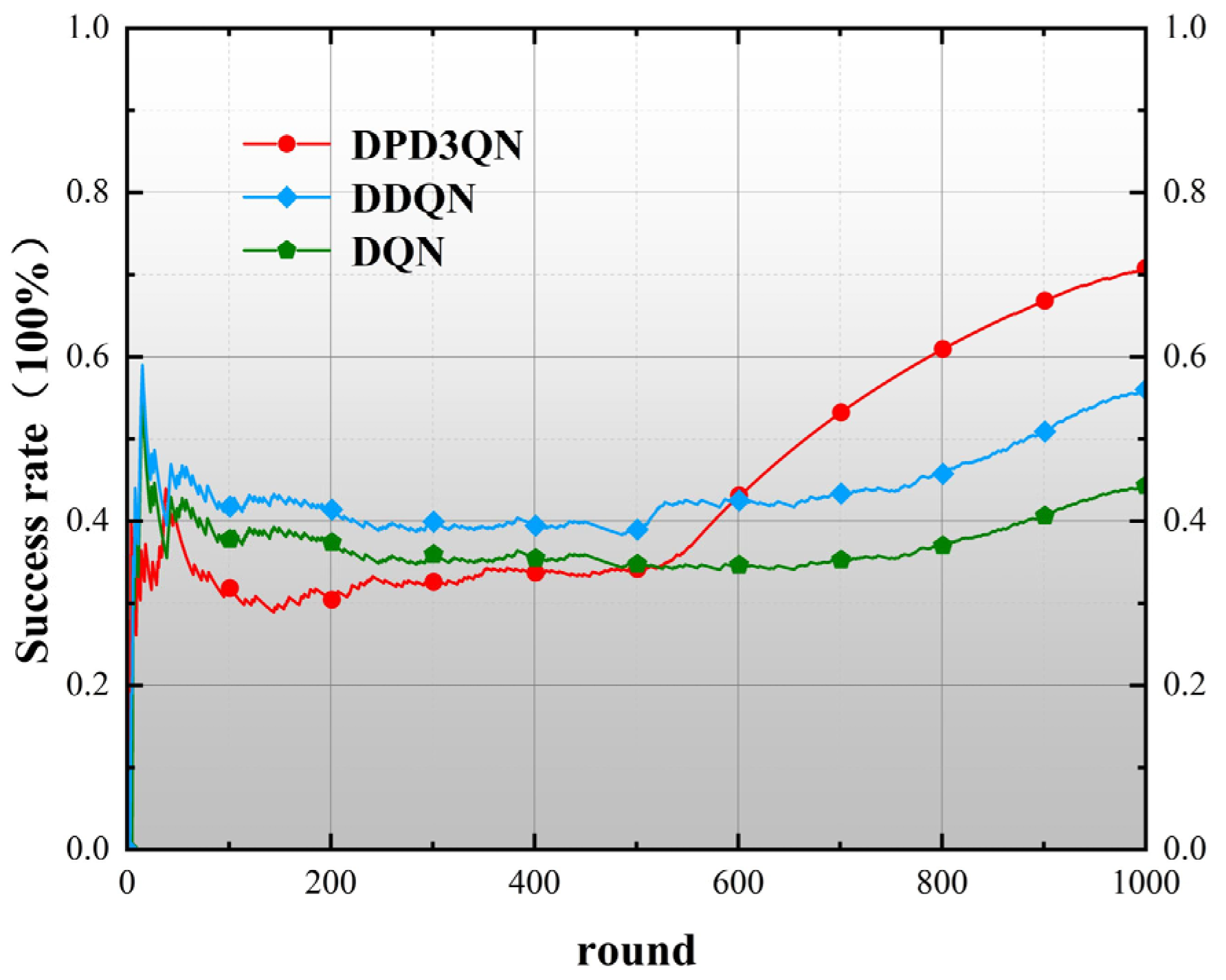
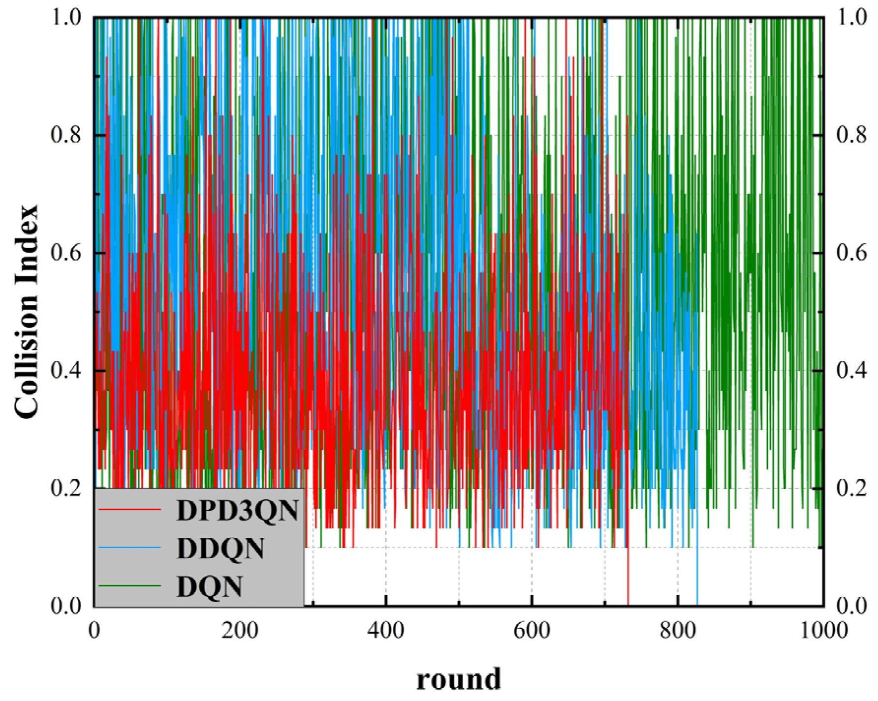
(3) After detailed training and testing experiments, it is verified that this method is superior to traditional deep reinforcement learning methods in terms of convergence speed and security. Through extensive experiments in multiple standardized environments, it is proven that DPD3QN significantly improves learning efficiency, decision-making quality, and stability compared with the existing technologies and can effectively cope with complex and challenging scenarios in autonomous driving.

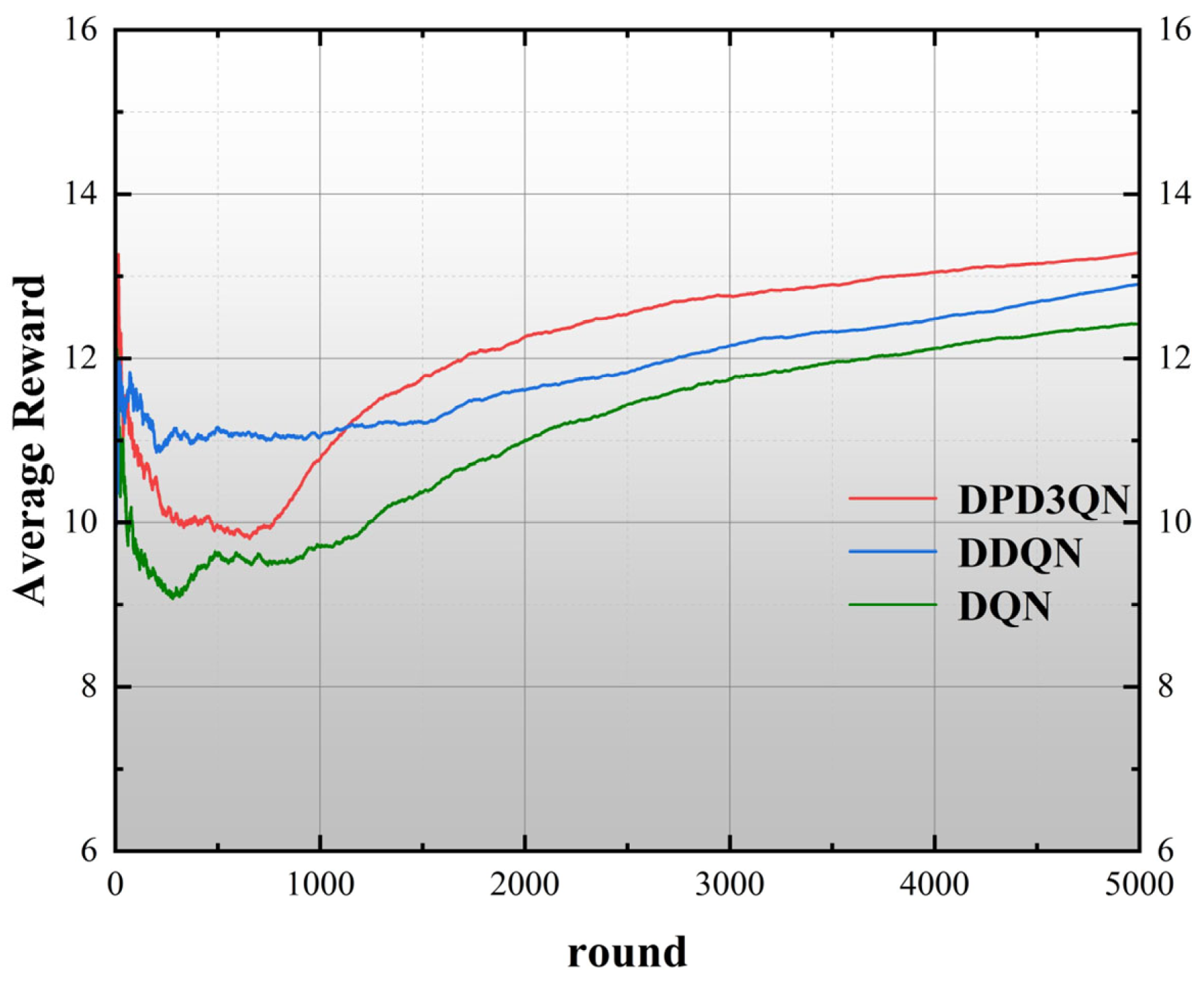
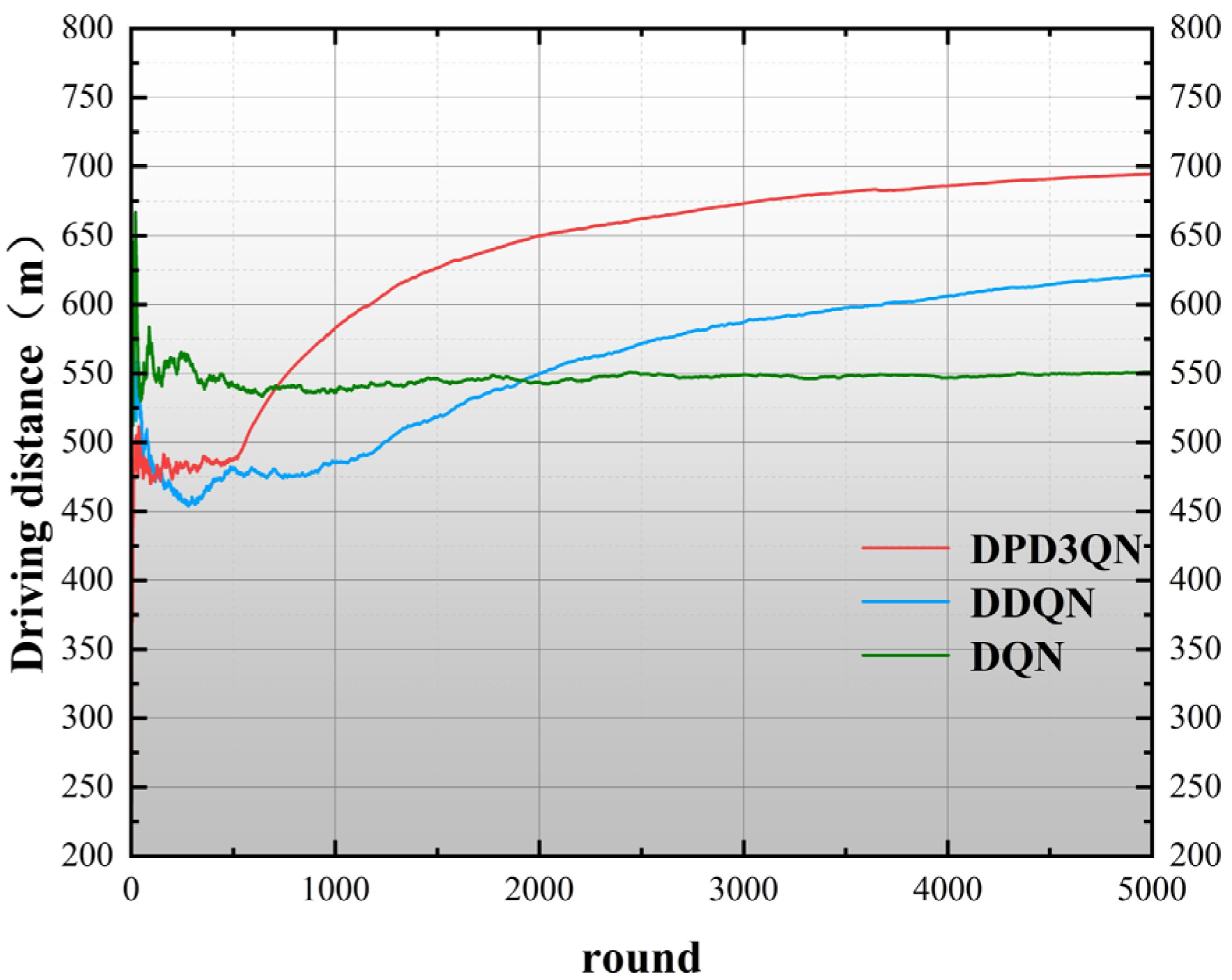
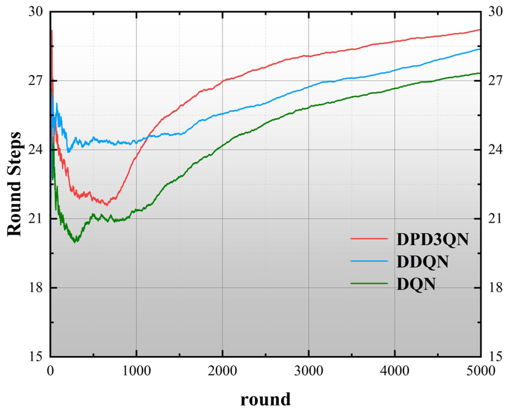
The experimental results show that compared with DDQN and DQN algorithms, DPD3QN improves the decision success rate by 11.8 and 25.8 percentage points in scenario I and by 8.8 and 22.2 percentage points in scenario II, respectively. In addition, DPD3QN also outperforms the comparison algorithms in terms of average reward and average driving speed, further demonstrating its advantages in complex driving tasks.

The realism of the simulation environment is limited, and the generalization capability to real-world scenarios still needs to be validated. Gaps remain compared to real road environments in terms of perception errors, behavioral uncertainty, and the complexity of traffic rules. Future research could incorporate higher-fidelity simulation platforms (such as CARLA or LGSVL) or real-world driving data for further validation. The modeling capability for multi-agent interactions needs to be improved. The current method primarily focuses on single-vehicle decision-making tasks and does not fully account for the dynamic impact of complex games and collaborative behaviors among multiple vehicles.