Quantifying Intra- and Inter-Observer Variabilities in Manual Contours for Radiotherapy: Evaluation of an MR Tumor Autocontouring Algorithm for Liver, Prostate, and Lung Cancer Patients

Abstract

Real-time tumor-tracked radiotherapy with a linear accelerator-magnetic resonance (linac-MR) hybrid system requires accurate tumor delineation at a fast MR imaging rate. Various autocontouring methods have been previously evaluated against “gold standard” manual contours by experts. However, manually drawn contours have inherent intra- and inter-observer variations. We aim to quantify these variations and evaluate our tumor-autocontouring algorithm against the manual contours. Ten liver, ten prostate, and ten lung cancer patients were scanned using a 3 tesla (T) magnetic resonance imaging (MRI) scanner with a 2D balanced steady-state free precession (bSSFP) sequence at 4 frames/s. Three experts manually contoured the tumor in two sessions. For autocontouring, an in-house built U-Net-based autocontouring algorithm was used, whose hyperparameters were optimized for each patient, expert, and session (PES). For evaluation, (A) Automatic vs. Manual and (B) Manual vs. Manual contour comparisons were performed. For (A) and (B), three types of comparisons were performed: (a) same expert same session, (b) same expert different session, and (c) different experts, using Dice coefficient (DC), centroid displacement (CD), and the Hausdorff distance (HD). For (A), the algorithm was trained using one expert’s contours and its autocontours were compared to contours from (a)–(c). For Automatic vs. Manual evaluations (Aa–Ac), DC = 0.91, 0.86, 0.78, CD = 1.3, 1.8, 2.7 mm, and HD = 3.1, 4.6, 7.0 mm averaged over 30 patients were achieved, respectively. For Manual vs. Manual evaluations (Ba–Bc), DC = 1.00, 0.85, 0.77, CD = 0.0, 2.1, 2.8 mm, and HD = 0.0, 4.9, 7.2 mm were achieved, respectively. We have quantified the intra- and inter-observer variations in manual contouring of liver, prostate, and lung patients. Our PES-specific optimized algorithm generated autocontours with agreement levels comparable to these manual variations, but with high efficiency (54 ms/autocontour vs. 9 s/manual contour).

1. Introduction

In radiation therapy, continuous tumor motion presents a major challenge in accurately targeting the tumor while minimizing exposure of surrounding healthy tissues. This issue is further compounded when the tumor experiences substantial movement and shape deformation (e.g., up to 40 mm in superior–inferior, 15 mm in anterior–posterior, and 10 mm in left–right directions [1,2,3], with volume changes up to 20% and rotations up to 50 degrees with respect to each axis during normal breathing for lung tumors [4]). Recently, real-time magnetic resonance (MR)-guided radiotherapy has become feasible through the development of novel hybrid systems known as linac-MR [5,6,7,8], which combine a radiotherapy device called a linear accelerator and the imaging capability of MRI. These systems enable real-time MR imaging of the tumor region with high soft-tissue contrast during irradiation, offering the potential to achieve non-invasive intrafractional tumor-tracked radiotherapy (nifteRT) [9,10,11,12]. nifteRT is a novel radiotherapy approach under development in which the therapeutic radiation beam dynamically tracks the motion of the tumor in real time, guided by intrafractional MR imaging. This is achieved by continuously adjusting the beam’s shape and position using multi-leaf collimator (MLC) control. The feasibility of nifteRT was first demonstrated in a phantom study by Yun et al. [9]. Further details on the development and validation of nifteRT can be found in Reference [9].

For nifteRT using a linac-MR, the initial step is to identify the tumor’s shape and position in each MR image. According to the American Association of Physicists in Medicine (AAPM) Task Group 76 report [13], a maximum delay of 500 ms is recommended between detecting the tumor’s position and delivering the beam once the MLC aligns with the tumor. This delay includes the time for image acquisition, reconstruction, contouring, and MLC repositioning. For image acquisition and reconstruction, ideally, a 3D image volume is acquired to capture any 3D motion of the tumor. However, techniques used for 3D imaging have long acquisition and reconstruction times (>400 ms) [14,15], which are not suitable for real-time tracking. Hence, we have chosen to use fast 2D MR imaging at ~4 frames/s for nifteRT.

For contouring, the clinical gold standard for tumor detection is manual contouring by experts. Since it is not feasible for a human expert to contour images at the fast imaging rate of linac-MR for the duration of treatment, various real-time autocontouring methods have been previously developed [9,16,17,18,19,20]. These methods are based on template matching, deformable image registration (DIR), and neural networks. Template-matching methods use a pre-defined template and a comparison metric (e.g., cross-correlation) to determine the best possible location of the template within the search image [21]. Thus, these methods assume the same tumor shape from the dynamic images. The DIR methods include B-splines [22] and demons [23,24]. Compared to template-matching and neural network-based methods, DIR methods may perform worse for tracking a tumor with large motion, as they typically assume small motion in the sequence of dynamic images [23]. More recently, neural network-based methods have been used, which include pulse-coupled neural network [16] and U-Net [25]. In contrast to the template matching methods, these methods contour the tumor within each dynamic image, detecting any real-time changes in tumor shape. Also, they have shown superior performance compared to the DIR with B-splines, which generally require only one reference image [18]. With these advantages of neural networks, this study used an in-house U-Net-based autocontouring algorithm.

Once an autocontouring algorithm is developed, proper assessment of the algorithm must follow. Currently, prior to radiotherapy planning, autocontours generated by commercially available algorithms (e.g., Limbus [26], MIM [27]) are generally used as a starting point for subsequent manual edits by experts. However, these algorithms cannot be used for nifteRT, during which real-time manual edits are not possible. For algorithms with higher contouring accuracy and speed (i.e., greater potential to be used for nifteRT), proper assessment of their contouring accuracy can still be difficult, as there is currently no set value for a clinically acceptable contouring accuracy. For instance, the autocontouring algorithm by Yun et al. [16] achieved mean Dice coefficients (DCs) of 0.87–0.92 between manual and autocontours for lung cancer patients. However, we are not able to determine whether the algorithm can be utilized in clinics. Since manual contours by human experts are the current clinical standard for tumor contouring, one way of determining this is to compare contouring performance against experts’ inherent uncertainties (i.e., intra- and inter-observer variations). In the literature, studies have investigated intra- and inter-observer variations in manual contours for 3D imaging of various sites within patients [28,29,30]. Molière et al. [28] estimated inter-observer variation in manual contours for 3D prostate MR images, which was found to be 0.919 in terms of DC. In the study by Cunha et al. [29], intra- and inter-observer variations for 3D MRI of tumor vasculature were reported with Jaccard Index values of 0.870 and 0.630, respectively. Also, intra- and inter-observer variations using 2D cine MR images have been previously investigated for some tumor sites [31,32]. In the study by Palacios et al. [31], inter-observer variation in manual contours for cine MR images of patients with lung, pancreatic, renal, and adrenal tumors was found to be 0.89 in terms of DC, averaged over all patients. However, intra- and inter-observer variations have not yet been quantified for 2D cine MR images of liver and prostate cancer patients. Those variations for lung patients have also not been quantified using numerous patient datasets. In addition, these three tumor sites have the potential for a large range of intrafractional tumor motion (up to 40 mm for lung [1] and liver [33], and 18 mm for prostate [34]) maximizing the clinical impact of nifteRT, while they also constitute a great portion of the radiotherapy patient population (~43% of all patients at our institution). Therefore, the primary aim of this study is to quantify intra- and inter-observer variations in manual contours for each of these tumor sites, and the secondary aim is to evaluate our tumor-autocontouring algorithm against the manual contours from multiple experts.

In this work, three experts (radiation oncologists) performed manual contouring of the tumor in dynamic MR images of 10 liver, 10 prostate, and 10 lung patients in two different sessions (300 images per patient, ~1-h tumor contouring per patient, and >20 weeks between sessions). An in-house-built tumor-autocontouring algorithm was optimized and trained for each patient, expert, and session (PES) to generate autocontours. The contours were subsequently evaluated by performing Automatic vs. Manual and Manual vs. Manual contour comparisons. With the tumors being patient-specific and the contours being PES-specific, customization of the autocontouring algorithm through the PES-specific optimization can largely improve the performance of the algorithm compared to using a single, general algorithm across all PESs. We hypothesize that our algorithm can generate tumor autocontours in each MR image within a range of tens of milliseconds, whose evaluation metrics against the manual contours are comparable to the manual intra- and inter-observer variation metrics.

2. Materials and Methods

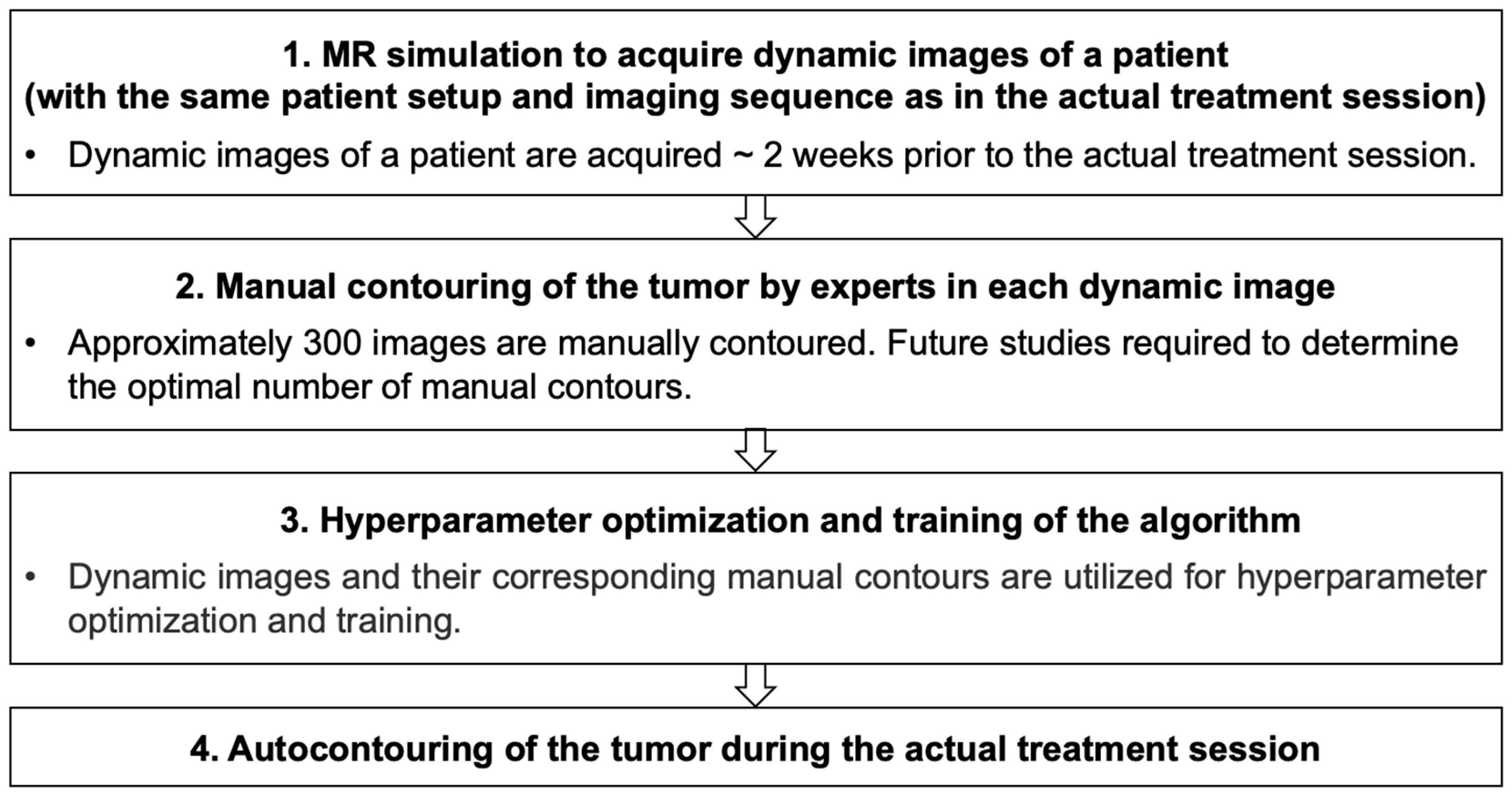
2.1. Patient Imaging and Manual Contouring

In this ethics-approved study, 30 cancer patients (10 liver, 10 prostate, and 10 lung) were recruited and scanned between 17 April 2013 and 15 June 2022 using a 3 tesla (T) magnetic resonance imaging (MRI) scanner (Philips Achieva, Eindhoven, the Netherlands) with a 2D balanced steady-state free precession (bSSFP) sequence (field of view = 30 $\times$ 40 to 40 $\times$ 40 cm², acquisition matrix size = 128 $\times$ 128, reconstructed matrix size = 256 $\times$ 256, voxel size = 2.3 $\times$ 3.1 $\times$ 10 − 3.1 $\times$ 3.1 $\times$ 15 mm³, echo time = 1.1 ms, repetition time = 2.2 ms, and imaging time per frame = 275 ms) to acquire ~ 500 dynamic images per patient (with an approximately 2 min imaging time). Only patients who were undergoing radiotherapy treatment, had no contraindication to MRI nor hip prostheses, and provided signed informed consent were included. Patients with liver, prostate, or lung cancer were included as they have the potential for significant intrafractional tumor motion and represent a large portion of the radiotherapy patient population (~43% of all patients at our institution). Patient characteristics can be found in

Table 1. Characteristics of the liver, prostate (sagittal: Patient (P) 11–16, axial: P17–18, coronal: P19–20), and lung cancer patients included in the study. If primary cancer site is different from site, it means it metastasized to site, which was imaged. F: female; M: male; N/A: not available; HCC: hepatocellular carcinoma; NSCLC: non-small cell lung cancer; SCLC: small cell lung cancer; SD: standard deviation.

Site	Patient	Gender	Age	Tumor Area (cm2)	Overall Stage	TNM Stage	Primary Cancer
Liver	1	F	65	36.2	III	TXNXM1	Rectal adenocarcinoma
	2	M	56	0.9	II	N/A	HCC
	3	M	70	24.2	IV	pT4pN2MX	Sigmoid colon adenocarcinoma
	4	M	57	2.8	I	N/A	HCC
	5	M	64	2.0	II	N/A	HCC
	6	M	63	3.7	IVB	T2N1M1	Nasopharyngeal carcinoma
	7	M	65	3.1	IVA	T3N2M1	Colorectal carcinoma
	8	M	59	2.4	IV	T3N0M1	Rectal adenocarcinoma
	9	M	68	1.5	IIB	TXNXM1	Rectal adenocarcinoma
	10	F	82	6.0	IV	T3N2M1	Colorectal cancer
Prostate	11	M	69	25.0	IIA	T1c	Prostatic adenocarcinoma
	12	M	69	24.4	IIA	T1c	Prostatic adenocarcinoma
	13	M	69	8.4	IIIC	T3aN0M0	Prostatic adenocarcinoma
	14	M	69	8.4	IIIC	T3aN0M0	Prostatic adenocarcinoma
	15	M	73	14.8	IIB	N/A	Prostatic adenocarcinoma
	16	M	73	12.8	IIB	N/A	Prostatic adenocarcinoma
	17	M	69	33.1	IIA	T1c	Prostatic adenocarcinoma
	18	M	75	26.4	IIB	T1c	Prostatic adenocarcinoma
	19	M	68	15.0	IIB	T1c	Prostatic adenocarcinoma
	20	M	77	18.9	IIIA	T1c	Prostatic adenocarcinoma
Lung	21	M	81	1.3	I	T1N0M0	NSCLC
	22	M	79	3.8	I	pT2pN1pMX	NSCLC
	23	F	73	6.4	II	T2N0M0	NSCLC
	24	M	72	4.8	IVA	T1NXM1a	NSCLC
	25	F	78	7.4	I	T1N0M0	Lung cancer unspecified
	26	M	65	1.4	IA	T1N0M0	NSCLC
	27	M	65	5.1	I	cT1cN0M0	NSCLC
	28	M	70	1.7	IB	N0M0	SCLC
	29	M	75	3.0	IIA	T2bN0M0	NSCLC
	30	M	65	3.8	IA	T1bN0M0	NSCLC
Mean (SD)				10.3 (10.4)

. Patients were imaged for research purposes without the use of gadolinium contrast agents.

In this retrospective study, each of the three radiation oncology experts manually contoured the gross tumor volume (GTV) in 300 dynamic images per patient (Session 1). To ensure independence, each expert was blinded to the contours drawn by the other two experts. Subsequently, they recontoured the same images (Session 2) approximately 20 weeks after Session 1 to prevent contouring from memory. All manual contouring was performed using the freely available 3D Slicer software (version 4.11) [35]. This software has the capability of importing 2D time series images and offers a variety of contouring tools. Since 3D Slicer is not the standard contouring software used in the clinic, the experts were given training to familiarize them with the software for the given tasks. In summary, a total of 54,000 images (30 patients $\times$ 3 experts $\times$ 2 sessions $\times$ 300 images) were manually contoured and used for this study.

2.2. Autocontouring Algorithm

A tumor-autocontouring algorithm [36] has been developed in-house using a U-Net architecture [25], whose hyperparameters are optimized with Covariance Matrix Adaptation Evolution Strategy (CMA-ES) [37]. Compared to the previous version of the algorithm based on pulse-coupled neural networks [32], this algorithm, originally developed by Yun et al. [38] and further improved by Han et al. [36], is more robust, having the capability of autocontouring challenging tumor sites such as the liver and prostate. As shown by Han et al. [36], the algorithm also outperformed the standardized segmentation algorithms, including non-optimized U-Net [25] and nnU-Net [39].

CMA-ES is a stochastic, population-based optimization technique designed for the real-parameter optimization of non-linear, non-convex functions. The optimization process begins by generating a population of candidate solutions sampled randomly from a normal distribution. After evaluating the objective function of each solution, the best portion of the population is chosen, and the corresponding covariance matrix is computed to modify the shape of the next sampling distribution. This allows the search to move in the directions of the previously successful steps, potentially leading to rapid convergence to the global minimum.

As the clinical standard for tumor segmentation is manual contouring by experts, the algorithm design accounts for the contouring tendencies of each expert in each session for a patient. This is achieved through PES-specific hyperparameter optimization (HPO) and training of the algorithm. The set of six hyperparameters—the number of consecutive convolutions before or after each pooling or up-convolution, filter size for convolutions, the number of feature maps, the number of poolings, the initial learning rate of the Adam optimizer, and the number of training images—was independently optimized for each PES within specified search ranges to obtain a PES-specific U-Net model. With 30 patients, 3 experts, and 2 sessions involved in this study, a total of 180 different PES-specific U-Net models were obtained.

A potential clinical workflow for implementing the algorithm is shown in Figure 1. The overall aim of HPO and training (step #3 in Figure 1) was to achieve ≥ 0.9 contouring accuracy from the testing images, measured by DC (∊[0, 1], where 1 represents complete agreement) between manual contours and autocontours. Since the mean (standard deviation (SD)) of intra- and inter-observer variations in experts’ manual contouring for lung cancer patients were previously found to be 0.88 (0.04) and 0.87 (0.04), respectively [32], a comparable number of 0.9 was set as a goal to determine reasonable autocontouring accuracy. The HPO and training process starts with the first iteration, in which 10 hyperparameter sets (solutions) are sampled using CMA-ES. The size of the solution population for CMA-ES was maintained at 10 for faster execution time for all PES cases. Each solution is then used to construct a modified U-Net, which is subsequently trained using the Dice loss function. The number of epochs for the training process of each solution is determined by an early-stopping method. This method was implemented to prevent the networks from overfitting to the training images, rather than generalizing to all imaging data (training, validation, and testing images). The early-stopping point (optimal number of epochs) below 15,000 is found for each solution by monitoring the validation accuracy. This process was terminated after 10 iterations for the entire solution population, which resulted in a validation accuracy of ~0.9 for all PES cases. The empirically determined training–validation–testing ratio of 160–70–70 was used in this study (with a search range of [10, 160] for the number of training images) for each PES-specific HPO and training, with the last 70 testing images unseen by the algorithm before testing. Although 300 dynamic images were manually contoured in this study, the optimal number of manual contours will be determined via further studies. More details on the algorithm can be found in Reference [36].

The algorithm was coded in Pytorch version 2.0.1 using the Python package, cma 2.7.0 on Google Colab (Ubuntu 22.04, Intel Xeon central processing unit (CPU), and 13 GB random access memory (RAM)). HPO and the training of the algorithm were run on an NVIDIA A100 graphics processing unit (GPU). The code will be available upon request for academic purposes.

2.3. Evaluation of Contours

For our evaluation of contours, we performed Automatic vs. Manual and Manual vs. Manual contour comparisons. For each of these comparisons, 3 distinct types of comparisons were performed: same-expert same-session (SESS) match, same-expert different-session (SEDS) match, and different-experts (DE) match. For Automatic vs. Manual comparisons, the autocontours generated by our algorithm (PES-specific optimized and trained) were compared against manual contours from each of the SESS, SEDS, and DE.

As previously mentioned, each PES dataset consisted of 300 images, which were divided into 160 for training, 70 for validation, and 70 for testing. For the Automatic vs. Manual SESS match, the algorithm was trained using manual contours drawn by an expert from a single session (utilizing 160 training and 70 validation images). The trained algorithm then generated autocontours for the 70 unseen testing images. For evaluation, these autocontours were compared against the expert’s manual contours from the same session. Therefore, the training, testing, and evaluation of the algorithm were all based on contours drawn during one session by an expert.

On the other hand, for the Automatic vs. Manual SEDS match, the algorithm was similarly trained on manual contours from a single session (160 training and 70 validation images) and generated autocontours on 70 testing images. However, for evaluation, the resulting autocontours were compared against the expert’s manual contours drawn during a different session. Thus, while training and testing were based on contours drawn during one session by an expert, the evaluation was performed using contours drawn in a different session. This setup enabled the assessment of the algorithm’s performance in the context of intra-observer variability.

For the Automatic vs. Manual DE match, the algorithm was trained using an expert’s manual contours and the autocontours were compared to a different expert’s contours. For both Automatic vs. Manual and Manual vs. Manual comparisons, the SEDS match represents intra-observer variabilities, while the DE match represents inter-observer variabilities.

For quantitative comparisons, three evaluation metrics were chosen based on the metric selection guidelines by Taha et al. [40]. First, DC [41] was used, defined as:

$$DC=2{\displaystyle \frac{Area\left(RO{I}_A\cap RO{I}_B\right)}{Area\left(RO{I}_A\right)+Area\left(RO{I}_B\right)}}$$

(1)

where $RO{I}_A$ and $RO{I}_B$ are contours A and B, respectively. DC measures the agreement between two contours based on their overlap. This makes DC robust to outlier contours, such as small islands that are irrelevant to the tumor contour [40]. However, DC has a limitation: when comparing small contours, even a slight change in the intersecting area (e.g., a few pixels) can cause a significant change in the overall DC value. Conversely, for larger contours, the same slight change in the intersecting area results in a relatively smaller change in the DC value. Therefore, for evaluating small contours, which are those with at least one dimension being significantly smaller (e.g., <5%) than the corresponding image dimension, distance-based metrics are recommended over overlap-based metrics [40]. As indicated in Table 1, tumors of varying sizes were contoured in this study, and tumors with sizes of <5.1 cm² (i.e., tumors with one dimension < 5% of the image dimension 40 cm) were classified as small contours based on the study by Taha et al. [40]. Hence, centroid displacement (CD) and the Hausdorff distance (HD) [42] were also employed to address the limitations of DC. CD measures the distance between the centroid of one contour and that of the other contour, with the centroid defined as:

$$centroid=\left({\displaystyle \frac{{{\displaystyle \sum }}_{i=1}^n{x}_i}{n}}, {\displaystyle \frac{{{\displaystyle \sum }}_{i=1}^n{y}_i}{n}}\right)$$

(2)

where $x_i$ and $y_i$ are the coordinates of pixel $i$ in the contour, and $n$ is the total number of pixels in the contour. To compute the HD between contours A and B, the following steps were taken. For every point on contour A, the minimum distance to any point on contour B was determined. The maximum of these distances was denoted as $d\left(A,B\right)$. Similarly, for every point on contour B, the minimum distance to any point on contour A was determined. The maximum of these distances was denoted as $d\left(B,A\right)$. HD was then defined as:

$$HD=\max \left(d\left(A,B\right),d\left(B,A\right)\right)$$

(3)

Each of these metrics was calculated for 70 testing images per patient.

3. Results

The Automatic vs. Manual and Manual vs. Manual evaluation metrics averaged over 10 patients for each tumor site, as well as each of the SESS, SEDS, or DE matches, are summarized in

Table 2. Automatic vs. Manual and Manual vs. Manual evaluation metrics (Dice coefficient (DC), centroid displacement (CD), and Hausdorff distance (HD) averaged over 10 patients per tumor site, and averaged over each of the SESS, SEDS, or DE matches). SD: standard deviation.

			Same Expert, Same Session (SESS)				Same Expert, Different Session (SEDS)				Different Experts (DE)
			Mean	Median	SD	Worst	Mean	Median	SD	Worst	Mean	Median	SD	Worst
Liver	Automatic vs. Manual	DC	0.90	0.89	0.05	0.87	0.79	0.79	0.04	0.73	0.70	0.68	0.04	0.60
		CD (mm)	1.4	1.4	0.8	1.8	2.3	2.4	0.9	2.7	3.3	3.2	1.0	4.0
		HD (mm)	3.0	2.8	0.9	3.7	5.3	5.6	1.1	5.7	7.7	7.9	1.3	9.3
	Manual vs. Manual	DC	-	-	-	-	0.78	0.79	0.05	0.72	0.69	0.67	0.05	0.60
		CD (mm)	-	-	-	-	2.7	2.6	1.1	2.9	3.5	3.5	1.2	4.1
		HD (mm)	-	-	-	-	5.7	5.8	1.4	6.1	7.8	7.9	1.6	9.3
Prostate	Automatic vs. Manual	DC	0.95	0.95	0.01	0.94	0.93	0.93	0.01	0.92	0.87	0.88	0.02	0.82
		CD (mm)	1.2	1.1	0.6	2.0	1.7	1.7	0.7	2.6	2.8	2.8	0.7	3.4
		HD (mm)	3.6	3.3	0.9	4.9	5.1	5.3	0.9	6.3	7.9	7.6	1.0	10.5
	Manual vs. Manual	DC	-	-	-	-	0.92	0.92	0.02	0.91	0.87	0.87	0.02	0.83
		CD (mm)	-	-	-	-	1.7	1.4	0.8	2.5	2.8	2.9	0.8	3.4
		HD (mm)	-	-	-	-	5.3	5.1	1.1	6.9	7.9	7.5	1.2	10.6
Lung	Automatic vs. Manual	DC	0.89	0.89	0.05	0.87	0.85	0.84	0.05	0.81	0.76	0.76	0.04	0.68
		CD (mm)	1.3	1.3	0.7	1.6	1.5	1.6	0.8	2.0	2.0	2.0	0.9	2.4
		HD (mm)	2.6	2.5	0.9	3.1	3.2	3.4	1.0	4.1	5.4	5.5	1.1	6.4
	Manual vs. Manual	DC	-	-	-	-	0.84	0.81	0.06	0.80	0.75	0.75	0.05	0.66
		CD (mm)	-	-	-	-	1.8	1.9	1.0	2.2	2.2	2.3	1.1	2.6
		HD (mm)	-	-	-	-	3.6	3.7	1.1	4.3	5.8	5.8	1.4	6.6

. For liver patients, Automatic vs. Manual SESS, SEDS, and DE DCs were 0.90, 0.79, and 0.70, respectively, while Manual vs. Manual SEDS and DE DCs were 0.78 and 0.69, respectively. For prostate patients, Automatic vs. Manual SESS, SEDS, and DE DCs were 0.95, 0.93, and 0.87, respectively, while Manual vs. Manual SEDS and DE DCs were 0.92 and 0.87, respectively. Lastly, for lung patients, Automatic vs. Manual SESS, SEDS, and DE DCs were 0.89, 0.85, and 0.76, respectively, while Manual vs. Manual SEDS and DE DCs were 0.84 and 0.75, respectively. The best overall agreement was observed for prostate patients, whereas the worst agreement was observed for liver patients for most of the comparisons. Additionally, the Manual vs. Manual SEDS metrics were found to be better than the Manual vs. Manual DE metrics consistently for all tumor sites.

Averaged over all 30 patients, Automatic vs. Manual evaluation metrics for SESS, SEDS, and DE were DC = 0.91, 0.86, 0.78, CD = 1.3, 1.8, 2.7 mm, and HD = 3.1, 4.6, 7.0 mm, respectively. In terms of intra-observer variability, the Automatic vs. Manual SEDS metrics are DC = 0.86, CD = 1.8 mm, and HD = 4.6 mm, whereas the Manual vs. Manual SEDS metrics are DC = 0.85, CD = 2.1 mm, and HD = 4.9 mm. This indicates that the agreement between auto- and manual contours is similar to the agreement between manual contours from different sessions by an expert. In terms of inter-observer variability, the Automatic vs. Manual DE metrics are DC = 0.78, CD = 2.7 mm, and HD = 7.0 mm, whereas the Manual vs. Manual DE metrics are DC = 0.77, CD = 2.8 mm, and HD = 7.2 mm. This suggests that the agreement between auto- and manual contours is comparable to the agreement between manual and manual contours from different experts.

The detailed evaluation metrics are shown in

Table A1. Dice coefficient (DC), centroid displacement (CD; mm), and Hausdorff distance (HD; mm) (mean (standard deviation) of 10 liver patients) for comparing Automatic vs. Manual contours and Manual vs. Manual contours. Shaded elements represent SESS comparisons. Bolded elements represent SEDS comparisons. Underlined elements represent DE comparisons.

Liver, Automatic vs. Manual
	M11			M12			M21			M22			M31			M32
	DC	CD	HD	DC	CD	HD	DC	CD	HD	DC	CD	HD	DC	CD	HD	DC	CD	HD
A11	0.92 (0.04)	1.2 (0.7)	2.6 (0.8)	0.80 (0.03)	2.4 (0.7)	5.6 (0.9)	0.76 (0.06)	3.2 (1.3)	7.1 (1.7)	0.73 (0.05)	3.6 (1.1)	6.9 (1.4)	0.67 (0.04)	2.9 (0.9)	7.6 (1.1)	0.65 (0.04)	3.6 (0.9)	7.9 (1.1)
A12	0.78 (0.03)	2.3 (0.7)	5.6 (0.9)	0.93 (0.03)	1.2 (0.6)	2.7 (0.8)	0.79 (0.05)	3.0 (1.2)	6.3 (1.5)	0.78 (0.05)	3.1 (1.0)	6.6 (1.3)	0.60 (0.03)	3.5 (1.0)	9.0 (1.3)	0.66 (0.03)	3.2 (0.8)	9.3 (1.1)
A21	0.75 (0.04)	3.0 (0.8)	7.1 (1.1)	0.80 (0.04)	2.9 (0.8)	5.9 (1.1)	0.89 (0.04)	1.6 (1.0)	3.5 (1.2)	0.85 (0.05)	2.1 (1.0)	4.8 (1.5)	0.64 (0.04)	3.7 (1.0)	8.5 (1.1)	0.68 (0.04)	3.4 (0.9)	9.1 (1.1)
A22	0.75 (0.04)	2.9 (0.8)	6.5 (1.1)	0.80 (0.04)	2.5 (0.8)	5.8 (1.2)	0.86 (0.05)	2.1 (1.1)	4.4 (1.4)	0.89 (0.05)	1.8 (0.9)	3.7 (1.2)	0.63 (0.04)	4.0 (1.0)	8.3 (1.3)	0.71 (0.04)	3.2 (0.9)	8.1 (1.2)
A31	0.66 (0.05)	2.8 (0.8)	7.4 (1.1)	0.61 (0.03)	3.5 (0.8)	8.8 (1.2)	0.65 (0.05)	3.7 (1.2)	8.2 (1.7)	0.64 (0.05)	3.8 (1.1)	7.9 (1.4)	0.87 (0.06)	1.4 (0.8)	2.8 (0.9)	0.73 (0.05)	2.4 (0.8)	5.7 (1.0)
A32	0.66 (0.04)	3.3 (0.8)	7.8 (1.1)	0.67 (0.04)	2.9 (0.8)	9.2 (1.1)	0.70 (0.05)	3.6 (1.2)	8.9 (1.7)	0.72 (0.05)	3.2 (1.1)	7.6 (1.6)	0.74 (0.05)	2.7 (1.0)	5.6 (1.1)	0.87 (0.05)	1.4 (0.7)	2.7 (0.7)
Liver, Manual vs. Manual
	M11			M12			M21			M22			M31			M32
	DC	CD	HD	DC	CD	HD	DC	CD	HD	DC	CD	HD	DC	CD	HD	DC	CD	HD
M11	-	-	-	0.79 (0.04)	2.6 (0.8)	5.8 (1.0)	0.75 (0.06)	3.4 (1.3)	7.4 (1.7)	0.72 (0.05)	3.7 (1.2)	7.0 (1.5)	0.66 (0.05)	3.0 (1.0)	6.7 (1.4)	0.65 (0.05)	3.6 (1.0)	7.9 (1.3)
M12	0.79 (0.04)	2.6 (0.8)	5.8 (1.0)	-	-	-	0.78 (0.06)	3.1 (1.3)	6.4 (1.7)	0.78 (0.06)	3.0 (1.1)	6.6 (1.5)	0.60 (0.04)	3.6 (1.1)	9.0 (1.5)	0.66 (0.04)	3.1 (1.1)	9.3 (1.3)
M21	0.75 (0.06)	3.4 (1.3)	7.4 (1.7)	0.78 (0.06)	3.1 (1.3)	6.4 (1.7)	-	-	-	0.84 (0.06)	2.5 (1.3)	5.2 (1.9)	0.64 (0.06)	3.9 (1.4)	8.5 (1.8)	0.68 (0.05)	3.7 (1.3)	9.1 (1.8)
M22	0.72 (0.05)	3.7 (1.2)	7.0 (1.5)	0.78 (0.06)	3.0 (1.1)	6.6 (1.5)	0.84 (0.06)	2.5 (1.3)	5.2 (1.9)	-	-	-	0.63 (0.05)	4.1 (1.3)	8.2 (1.6)	0.71 (0.05)	3.3 (1.2)	7.8 (1.6)
M31	0.66 (0.05)	3.0 (1.0)	6.7 (1.4)	0.60 (0.04)	3.6 (1.1)	9.0 (1.5)	0.64 (0.06)	3.9 (1.4)	8.5 (1.8)	0.63 (0.05)	4.1 (1.3)	8.2 (1.6)	-	-	-	0.72 (0.06)	2.9 (1.1)	6.1 (1.4)
M32	0.65 (0.05)	3.6 (1.0)	7.9 (1.3)	0.66 (0.04)	3.1 (1.1)	9.3 (1.3)	0.68 (0.05)	3.7 (1.3)	9.1 (1.8)	0.71 (0.05)	3.3 (1.2)	7.8 (1.6)	0.72 (0.06)	2.9 (1.1)	6.1 (1.4)	-	-	-

,

Table A2. Dice coefficient (DC), centroid displacement (CD; mm), and Hausdorff distance (HD; mm) (mean (standard deviation) of 10 prostate patients) for comparing Automatic vs. Manual contours and Manual vs. Manual contours. Shaded elements represent SESS comparisons. Bolded elements represent SEDS comparisons. Underlined elements represent DE comparisons.

Prostate, Automatic vs. Manual
	M11			M12			M21			M22			M31			M32
	DC	CD	HD	DC	CD	HD	DC	CD	HD	DC	CD	HD	DC	CD	HD	DC	CD	HD
A11	0.96 (0.01)	0.7 (0.4)	2.7 (0.7)	0.95 (0.01)	1.2 (0.4)	3.8 (0.6)	0.88 (0.02)	2.4 (0.8)	7.3 (1.3)	0.85 (0.02)	3.2 (0.9)	9.0 (1.3)	0.89 (0.02)	2.5 (0.7)	6.4 (1.1)	0.89 (0.02)	2.9 (0.5)	6.8 (0.8)
A12	0.94 (0.01)	1.5 (0.4)	4.1 (0.7)	0.96 (0.01)	0.8 (0.3)	2.7 (0.7)	0.87 (0.02)	2.4 (0.8)	7.7 (1.3)	0.85 (0.02)	2.9 (1.0)	9.0 (1.3)	0.89 (0.02)	2.9 (0.8)	6.4 (0.9)	0.88 (0.01)	3.1 (0.5)	6.6 (0.9)
A21	0.88 (0.01)	2.2 (0.5)	7.3 (0.7)	0.88 (0.01)	2.1 (0.6)	7.4 (0.8)	0.94 (0.02)	1.7 (0.8)	4.6 (1.3)	0.92 (0.02)	2.6 (1.1)	6.3 (1.4)	0.84 (0.02)	2.7 (0.8)	9.2 (1.3)	0.88 (0.01)	2.9 (0.7)	8.4 (1.2)
A22	0.85 (0.01)	2.2 (0.5)	8.3 (0.7)	0.86 (0.01)	2.0 (0.4)	8.2 (0.7)	0.92 (0.02)	2.1 (0.9)	6.1 (1.4)	0.94 (0.02)	2.0 (0.9)	4.9 (1.4)	0.82 (0.02)	3.1 (0.8)	10.5 (1.3)	0.86 (0.01)	3.3 (0.6)	9.8 (0.9)
A31	0.89 (0.01)	2.5 (0.5)	6.2 (0.7)	0.89 (0.01)	2.8 (0.5)	6.0 (0.7)	0.86 (0.02)	2.4 (0.8)	8.4 (1.4)	0.83 (0.02)	3.3 (0.9)	10.4 (1.4)	0.95 (0.01)	1.1 (0.6)	3.3 (0.8)	0.93 (0.01)	1.3 (0.5)	5.1 (0.7)
A32	0.88 (0.01)	3.2 (0.4)	7.3 (0.6)	0.88 (0.01)	3.2 (0.5)	6.8 (0.7)	0.89 (0.02)	2.7 (0.8)	7.5 (1.2)	0.87 (0.02)	3.4 (0.8)	9.7 (1.3)	0.92 (0.01)	1.5 (0.7)	5.4 (0.8)	0.95 (0.01)	1.1 (0.5)	3.3 (0.6)
Prostate, Manual vs. Manual
	M11			M12			M21			M22			M31			M32
	DC	CD	HD	DC	CD	HD	DC	CD	HD	DC	CD	HD	DC	CD	HD	DC	CD	HD
M11	-	-	-	0.94 (0.01)	1.4 (0.5)	4.0 (0.7)	0.88 (0.02)	2.3 (0.8)	7.3 (1.3)	0.85 (0.02)	3.1 (0.9)	9.1 (1.3)	0.89 (0.02)	2.5 (0.7)	6.4 (0.9)	0.88 (0.01)	2.9 (0.6)	6.7 (0.8)
M12	0.94 (0.01)	1.4 (0.5)	4.0 (0.7)	-	-	-	0.88 (0.02)	2.4 (0.9)	7.5 (1.3)	0.86 (0.02)	2.9 (1.0)	8.8 (1.3)	0.89 (0.02)	2.8 (0.8)	6.2 (0.9)	0.89 (0.01)	3.1 (0.6)	6.4 (0.9)
M21	0.88 (0.02)	2.3 (0.8)	7.3 (1.3)	0.88 (0.02)	2.4 (0.9)	7.5 (1.3)	-	-	-	0.91 (0.02)	2.5 (1.2)	6.9 (1.9)	0.85 (0.02)	2.4 (0.8)	8.4 (1.4)	0.89 (0.02)	2.5 (0.9)	7.4 (1.5)
M22	0.85 (0.02)	3.1 (0.9)	9.1 (1.3)	0.86 (0.02)	2.9 (1.0)	8.8 (1.3)	0.91 (0.02)	2.5 (1.2)	6.9 (1.9)	-	-	-	0.83 (0.02)	3.4 (1.1)	10.6 (1.6)	0.87 (0.02)	3.3 (0.9)	9.9 (1.5)
M31	0.89 (0.02)	2.5 (0.7)	6.4 (0.9)	0.89 (0.02)	2.8 (0.8)	6.2 (0.9)	0.85 (0.02)	2.4 (0.8)	8.4 (1.4)	0.83 (0.02)	3.4 (1.1)	10.6 (1.6)	-	-	-	0.92 (0.01)	1.3 (0.6)	5.1 (0.8)
M32	0.88(0.01)	2.9 (0.6)	6.7 (0.8)	0.89 (0.01)	3.1 (0.6)	6.4 (0.9)	0.89 (0.02)	2.5 (0.9)	7.4 (1.5)	0.87 (0.02)	3.3 (0.9)	9.9 (1.5)	0.92 (0.01)	1.3 (0.6)	5.1 (0.8)	-	-	-

and

Table A3. Dice coefficient (DC), centroid displacement (CD; mm), and Hausdorff distance (HD; mm) (mean (standard deviation) of 10 lung patients) for comparing Automatic vs. Manual contours and Manual vs. Manual contours. Shaded elements represent SESS comparisons. Bolded elements represent SEDS comparisons. Underlined elements represent DE comparisons.

Lung, Automatic vs. Manual
	M11			M12			M21			M22			M31			M32
	DC	CD	HD	DC	CD	HD	DC	CD	HD	DC	CD	HD	DC	CD	HD	DC	CD	HD
A11	0.92 (0.03)	1.0 (0.6)	2.3 (0.7)	0.91 (0.04)	1.1 (0.6)	2.5 (0.8)	0.82 (0.05)	2.2 (1.0)	5.0 (1.4)	0.82 (0.04)	2.0 (1.0)	5.0 (1.3)	0.77 (0.05)	2.0 (0.9)	5.4 (1.1)	0.73 (0.04)	1.6 (0.7)	5.8 (1.0)
A12	0.90 (0.03)	1.1 (0.6)	2.5 (0.7)	0.92 (0.03)	1.0 (0.6)	2.3 (0.7)	0.82 (0.05)	2.4 (1.0)	5.1 (1.4)	0.82 (0.04)	2.2 (1.0)	5.2 (1.4)	0.75 (0.05)	2.0 (0.9)	5.7 (1.1)	0.70 (0.04)	1.8 (0.7)	6.1 (0.9)
A21	0.86 (0.04)	1.9 (0.9)	4.2 (1.2)	0.85 (0.04)	2.0 (0.8)	4.5 (1.1)	0.87 (0.05)	1.6 (0.8)	3.1 (1.1)	0.84 (0.04)	1.8 (0.9)	3.6 (1.1)	0.76 (0.05)	2.0 (1.0)	5.0 (1.1)	0.71 (0.04)	1.6 (0.8)	5.1 (1.1)
A22	0.83 (0.04)	1.9 (0.8)	4.6 (1.1)	0.83 (0.04)	2.0 (0.8)	4.9 (1.1)	0.82 (0.05)	2.0 (1.0)	4.1 (1.2)	0.89 (0.05)	1.5 (0.9)	2.9 (1.1)	0.72 (0.04)	2.4 (1.0)	5.7 (1.0)	0.68 (0.04)	1.9 (0.7)	5.8 (0.9)
A31	0.77 (0.05)	1.7 (0.7)	5.6 (1.1)	0.76 (0.04)	1.8 (0.7)	5.9 (1.0)	0.75 (0.05)	2.1 (1.0)	5.2 (1.3)	0.72 (0.04)	2.2 (1.0)	5.8 (1.2)	0.87 (0.06)	1.4 (0.8)	2.7 (0.9)	0.83 (0.05)	1.5 (0.7)	3.1 (0.9)
A32	0.74 (0.04)	1.6 (0.7)	6.1 (1.1)	0.72 (0.04)	1.7 (0.8)	6.4 (1.0)	0.71 (0.05)	1.8 (0.9)	5.5 (1.3)	0.68 (0.04)	2.1 (1.0)	6.0 (1.2)	0.81 (0.06)	1.7 (0.9)	3.6 (1.1)	0.89 (0.05)	1.1 (0.6)	2.1 (0.7)
Lung, Manual vs. Manual
	M11			M12			M21			M22			M31			M32
	DC	CD	HD	DC	CD	HD	DC	CD	HD	DC	CD	HD	DC	CD	HD	DC	CD	HD
M11	-	-	-	0.90 (0.04)	1.3 (0.7)	2.8 (0.8)	0.81 (0.05)	2.4 (1.1)	5.2 (1.5)	0.81 (0.05)	2.2 (1.2)	5.3 (1.5)	0.76 (0.05)	2.1 (0.9)	5.8 (1.3)	0.72 (0.05)	1.8 (0.9)	6.2 (1.3)
M12	0.90 (0.04)	1.3 (0.7)	2.8 (0.8)	-	-	-	0.81 (0.06)	2.4 (1.1)	5.5 (1.5)	0.81 (0.05)	2.3 (1.2)	5.6 (1.6)	0.75 (0.05)	2.1 (0.9)	6.2 (1.2)	0.70 (0.05)	2.0 (0.9)	6.6 (1.2)
M21	0.81 (0.05)	2.4 (1.1)	5.2 (1.5)	0.81 (0.06)	2.4 (1.1)	5.5 (1.5)	-	-	-	0.81 (0.06)	2.2 (1.2)	4.3 (1.4)	0.74 (0.06)	2.4 (1.2)	5.5 (1.5)	0.70 (0.06)	2.1 (1.0)	5.7 (1.4)
M22	0.81 (0.05)	2.2 (1.2)	5.3 (1.5)	0.81 (0.05)	2.3 (1.2)	5.6 (1.6)	0.81 (0.06)	2.2 (1.2)	4.3 (1.4)	-	-	-	0.70 (0.05)	2.6 (1.2)	6.1 (1.3)	0.66 (0.05)	2.3 (1.1)	6.3 (1.3)
M31	0.76 (0.05)	2.1 (0.9)	5.8 (1.3)	0.75 (0.05)	2.1 (0.9)	6.2 (1.2)	0.74 (0.06)	2.4 (1.2)	5.5 (1.5)	0.70 (0.05)	2.6 (1.2)	6.1 (1.3)	-	-	-	0.80 (0.07)	1.9 (1.0)	3.7 (1.1)
M32	0.72(0.05)	1.8 (0.9)	6.2 (1.3)	0.70 (0.05)	2.0 (0.9)	6.6 (1.2)	0.70 (0.06)	2.1 (1.0)	5.7 (1.4)	0.66 (0.05)	2.3 (1.1)	6.3 (1.3)	0.80 (0.07)	1.9 (1.0)	3.7 (1.1)	-	-	-

in the Appendix A, in which the following notation is used: A₁₂ denotes autocontours generated by our algorithm, trained using manual contours from expert 1 in session 2. M₃₁ denotes manual contours drawn by expert 3 in session 1. In these tables, the mean (standard deviation) DC, CD, and HD values are displayed, where the shaded, diagonal elements are SESS comparisons, bolded elements are SEDS comparisons, and underlined elements are DE comparisons. For the Automatic vs. Manual comparisons, six sets of autocontours (A₁₁, A₁₂, A₂₁, A₂₂, A₃₁, and A₃₂) were compared against six sets of manual contours drawn on the same images, namely, M₁₁, M₁₂, M₂₁, M₂₂, M₃₁, and M₃₂. For the Manual vs. Manual comparisons, the manual contours (M₁₁, M₁₂, M₂₁, M₂₂, M₃₁, and M₃₂) were compared against each other.

Figure 2 shows patient cases with the best and worst Automatic vs. Manual and Manual vs. Manual intra- or inter-observer variability (i.e., SEDS or DE) DC for each tumor site. In this figure, examples of intra-observer variability DCs are shown for liver, while inter-observer variability DCs are shown for the prostate and lung. This is to show visual Automatic vs. Manual and Manual vs. Manual comparisons for both intra- and inter-observer variability comparisons. Comparing each of the Automatic vs. Manual with Manual vs. Manual comparisons, it can be visually confirmed that the agreement between auto- and manual contours is similar to the agreement between manual and manual contours.

4. Discussion

Intrafractional MR-guided radiotherapy demands accurate and fast tumor segmentation in each dynamic image. To implement a tumor-autocontouring algorithm, its accuracy must be evaluated against “gold standard” contours, which are currently expert-drawn but vary among experts and different sessions of an expert. Since there is no practical way to determine which set of expert-drawn contours is the actual truth, the accuracy of the “gold standard” can be indicated by intra- and inter-observer variations, which are unknown for cine MR images of liver and prostate cancer patients. This work quantified these variations to establish a clinically acceptable accuracy level for a tumor-autocontouring algorithm in intrafractional MR-guided radiotherapy.

Depending on clinical scenarios, an autocontouring algorithm can be trained and tested using either (i) an expert’s contours from different sessions, or (ii) different experts’ contours. For scenario (i), an autocontour can be considered acceptable if it has Automatic vs. Manual SEDS evaluation metrics comparable to Manual vs. Manual intra-observer variations. For scenario (ii), an autocontour can be considered acceptable if it has Automatic vs. Manual DE metrics comparable to Manual vs. Manual inter-observer variations. If those metrics are comparable in each scenario, we can claim that the algorithm faithfully imitates the contouring performance of the human experts and thus can be adopted for nifteRT. As shown in Table 2, the Automatic vs. Manual SEDS and DE metrics were similar to the Manual vs. Manual intra- and inter-observer variations, respectively. For example, the Automatic vs. Manual SEDS and DE DCs for liver (0.79 and 0.70) were 1% higher than the Manual vs. Manual SEDS and DE DCs (0.78 and 0.69). This demonstrates that the algorithm mimicked each expert’s contours with as much uncertainty as there is between different sessions or different experts.

The worst overall agreement was observed for liver patients, whereas the best agreement was observed for prostate patients for most of the comparisons. For the DC values, this can be due to the smaller size of the liver tumor (8.3 cm² on average) compared to the prostate (18.7 cm² on average) for most patient cases. Since DC is a percentage value of two contour areas, even a slight change in the intersecting area between two small contours leads to a large change in the overall DC value. In terms of HD, agreement was better for liver patients for the Automatic vs. Manual SESS and DE matches, as well as for the Manual vs. Manual DE match, as shown in Table 2. Also, another potential cause is the lower image contrast between the liver tumor and the normal tissue background for some patient cases. If the patients are imaged with the gadolinium contrast agent, the contouring performance of the algorithm and the experts, as well as their agreements, would likely be improved. In contrast, for both prostate and lung patients, the boundary between the prostate and its background (especially in coronal or axial plane images), as well as the lung tumor and its background, was quite clear without contrast enhancement.

The manual intra-observer agreements were found to be better than the manual inter-observer agreements consistently for all tumor sites, suggesting that the experts tend to agree more with themselves than with the other experts. This is consistent with what has been demonstrated in the literature [43,44,45]. Also, our manual intra-/inter-observer agreements differ from those in the previous tumor contouring studies. For lung patients, our agreements (mean DC: 0.84/0.75) are lower than those reported by Yip et al. (mean DC: 0.88/0.87) [32]. This discrepancy may be due to variations in study protocols, including different contouring software (3D Slicer vs. computational environment for radiotherapy research (CERR)) and numbers of patients (10 vs. 6 patients). For prostate patients, our agreements (mean DC: 0.92/0.87) are higher than those found by Lim et al. (mean DC: 0.80/0.80) [30]. Differences in imaging modality (MRI vs. computed tomography (CT)) and contouring image dimensions (2D vs. 3D) may account for this discrepancy. For liver patients, our agreements (mean DC: 0.78/0.69) are lower than those reported by Covert et al. (mean DC: 0.85/0.79) [46]. This difference can be attributed to variations in imaging planes (sagittal vs. axial) and the use of contrast enhancement (without vs. with enhancement). In addition, the relatively low manual intra-/inter-observer agreements found for the liver patients in this study may be due to the low tumor contrast and the fact that the contouring of GTV was based on what the radiation oncologists could visibly see on the images, taking into account their clinical judgment. Furthermore, upon comparing the Automatic vs. Manual SESS metrics, our agreements for lung patients (mean DC: 0.89 (0.05), HD: 2.6 (0.9) mm) were similar to those reported by Yip et al. (mean DC: 0.90 (0.03), HD: 3.8 (1.6) mm)) [32]. The algorithm used by Yip et al. [32] does not work for liver and prostate patients. Due to the substantive differences in the study protocols, any direct comparison between our results and those in the previous studies is not warranted.

To summarize, this work allows one to evaluate whether a given tumor-autocontouring algorithm can be as accurate as human experts’ contouring for different tumor sites and, thereby, determine whether it can be used clinically. With the fast contouring ability (54 ms/contour) compared to that of experts (~9 s/contour in this study), along with the similar contouring accuracy, the presented algorithm fulfills the crucial criteria for realizing nifteRT, which enables a treatment margin reduction without compromising tumor coverage. nifteRT has the potential to make a significant clinical impact in the treatment of abdominothoracic cancer patients who are unable to tolerate conventional motion management techniques, such as breath-hold or abdominal compression, yet still require tight treatment margins to avoid serious complications. For prostate cancer, nifteRT may offer real-time surveillance during radiation delivery, helping to reduce the risk of substantial geometric misses that could lead to severe bladder or rectal toxicities. Most importantly, nifteRT accomplishes this without the need for invasive surgical procedures. By allowing for both dose escalation to improve tumor control probability and margin reduction to minimize the risk of normal tissue complications, nifteRT could meaningfully enhance the therapeutic ratio and expand treatment options for patients with mobile or deformable tumors who currently have limited alternatives.

One limitation of this study is that the patients were imaged on a 3 T MRI system, although a linac-MR system typically operates at a lower field strength (e.g., 0.5 T for Alberta Linac-MR, 1.5 T for Elekta, 0.35 T for ViewRay) [5,6,7,8,47]. Hence, depending on the system used, the image quality (e.g., contrast-to-noise ratio (CNR), signal-to-noise ratio) will be different. However, regardless of the field strength used for imaging, the CNR will undoubtedly have an effect on contouring accuracy for both the experts and the algorithm alike. Rather than quantifying the results at a specific field strength, future work could investigate contouring accuracy with respect to the CNR, which could be useful for real-time tracking on all imaging sequences and field strengths. The algorithm’s performance with 0.5 T linac-MR images, as well as noise-added 3 T images, is currently being investigated. For the Alberta Linac-MR system, patient treatments and MR imaging are being performed in clinical trials.

Another limitation noted by one of the radiation oncologists is that during manual contouring, the pixels could not always conform to the tumor image, especially for small tumors. To reduce the pixelation effect, the 256 $\times$ 256 matrix size can be increased (e.g., to 512 $\times$ 512) by padding k-space data with zeros before taking the inverse Fourier transformation to the image domain. Alternatively, recent studies have investigated deep learning-based super-resolution networks [48,49], which could be a solution to improve the spatial resolution without compromising the temporal resolution. In addition, since manual contouring is a very onerous process, radiation oncologists may have accepted more errors for the non-clinical contours. Future studies could also benefit from including more patients, experts, and tumor sites.

5. Conclusions

We have quantified the intra- and inter-observer variations in manual contours for liver, prostate, and lung cancer patients imaged with 3 T MRI. These quantifications were used to evaluate our tumor-autocontouring algorithm, which was customized through patient-, expert-, and session-specific hyperparameter optimization and training. Consequently, the algorithm generated tumor autocontours that faithfully emulated the contouring tendencies of each expert, but with high efficiency (54 ms/contour). Moreover, the consistency between autocontours and manual contours was comparable to the manual intra- and inter-observer variabilities observed across liver, prostate, and lung cases.

References

1. Plathow, C.; Fink, C.; Ley, S.; Puderbach, M.; Eichinger, M.; Zuna, I.; Schmähl, A.; Kauczor, H.U. Measurement of tumor diameter-dependent mobility of lung tumors by dynamic MRI. Radiother. Oncol. 2004, 73, 349–354. [Google Scholar] [CrossRef] [PubMed]
2. Shirato, H.; Suzuki, K.; Sharp, G.C.; Fujita, K.; Onimaru, R.; Fujino, M.; Kato, N.; Osaka, Y.; Kinoshita, R.; Taguchi, H.; et al. Speed and amplitude of lung tumor motion precisely detected in fourdimensional setup and in real-time tumor-tracking radiotherapy. Int. J. Radiat. Oncol. Biol. Phys. 2006, 64, 1229–1236. [Google Scholar] [CrossRef]
3. Shirato, H.; Seppenwoolde, Y.; Kitamura, K.; Onimura, R.; Shimizu, S. Intrafractional tumor motion: Lung and liver. Semin. Radiat. Oncol. 2004, 14, 10–18. [Google Scholar] [CrossRef]
4. Plathow, C.; Klopp, M.; Fink, C.; Sandner, A.; Hof, H.; Puderbach, M.; Herth, F.; Schmähl, A.; Kauczor, H.U. Quantitative analysis of lung and tumour mobility: Comparison of two time-resolved MRI sequences. Br. J. Radiol. 2005, 78, 836–840. [Google Scholar] [CrossRef]
5. Fallone, B.G.; Murray, B.; Rathee, S.; Stanescu, T.; Steciw, S.; Vidakovic, S.; Blosser, E.; Tymofichuk, D. First MR images obtained during megavoltage photon irradiation from a prototype integrated linac-MR system. Med. Phys. 2009, 36, 2084–2088. [Google Scholar] [CrossRef] [PubMed]
6. Fallone, B.G. The rotating biplanarlinac magnetic resonance imaging system. Semin. Radiat. Oncol. 2014, 24, 200–202. [Google Scholar] [CrossRef]
7. Mutic, S.; Dempsey, J.F. The ViewRay system: Magnetic resonance-guided and controlled radiotherapy. Semin. Radiat. Oncol. 2014, 24, 196–199. [Google Scholar] [CrossRef] [PubMed]
8. Raaymakers, B.W.; Lagendijk, J.J.W.; Overweg, J.; Kok, J.G.M.; Raaijmakers, A.J.E.; Kerkhof, E.M.; van der Put, R.W.; Meijsing, I.; Crijins, S.P.M.; Benedosso, F.; et al. Integrating a 1.5 T MRI scanner with a 6 MV accelerator: Proof of concept. Phys. Med. Biol. 2009, 54, N229–N237. [Google Scholar] [CrossRef]
9. Yun, J.; Wachowicz, K.; Mackenzie, M.; Rathee, S.; Robinson, D.; Fallone, B.G. First demonstration of intrafractional tumor-tracked irradiation using 2D phantom MR images on a prototype linac-MR. Med. Phys. 2013, 40, 051718. [Google Scholar] [CrossRef]
10. Tacke, M.B.; Nill, S.; Krauss, A.; Oelfke, U. Real-time tumor tracking: Automatic compensation of target motion using the Siemens 160 MLC. Med. Phys. 2010, 37, 753–761. [Google Scholar] [CrossRef]
11. Cho, B.; Poulsen, P.R.; Sloutsky, A.; Sawant, A.; Keall, P.J. First demonstration of combined kV/MV image-guided real-time dynamic multileaf-collimator target tracking. Int. J. Radiat. Oncol. Biol. Phys. 2009, 74, 859–867. [Google Scholar] [CrossRef] [PubMed]
12. Sawant, A.; Venkat, R.; Srivastava, V.; Carlson, D.; Povzner, S.; Cattell, H.; Keall, P. Management of three-dimensional intrafraction motion through real-time DMLC tracking. Med. Phys. 2008, 35, 2050–2061. [Google Scholar] [CrossRef] [PubMed]
13. Keall, P.J.; Mageras, G.S.; Balter, J.M.; Emery, R.S.; Forster, K.M.; Jiang, S.B.; Kapatoes, J.M.; Low, D.A.; Murphy, M.J.; Murray, B.R.; et al. The management of respiratory motion in radiation oncology report of AAPM Task Group 76. Med. Phys. 2006, 33, 3874–3900. [Google Scholar] [CrossRef] [PubMed]
14. Kim, T.; Park, J.C.; Gach, H.M.; Chun, J.; Mutic, S. Technical note: Realtime 3D MRI in the presence of motion for MRI-guided radiotherapy: 3D dynamic keyhole imaging with super-resolution. Med. Phys. 2019, 46, 4631–4638. [Google Scholar] [CrossRef] [PubMed]
15. Bjerre, T.; Crijns, S.; af Rosenschöld, P.M.; Aznar, M.; Specht, L.; Larsen, R.; Keall, P. Three-dimensional MRI-linac intra-fraction guidance using multiple orthogonal cine-MRI planes. Phys. Med. Biol. 2013, 58, 4943–4950. [Google Scholar] [CrossRef]
16. Yun, J.; Yip, E.; Gabos, Z.; Wachowicz, K.; Rathee, S.; Fallone, B.G. Neural-network based autocontouring algorithm for intrafractional lung-tumor tracking using Linac-MR. Med. Phys. 2015, 42, 2296–2310. [Google Scholar] [CrossRef]
17. Bourque, A.E.; Bedwani, S.; Filion, É.; Carrier, J.F. A particle filter based autocontouring algorithm for lung tumor tracking using dynamic magnetic resonance imaging. Med. Phys. 2016, 43, 5161. [Google Scholar] [CrossRef]
18. Friedrich, F.; Hörner-Rieber, J.; Renkamp, C.K.; Klüter, S.; Bachert, P.; Ladd, M.E.; Knowles, B.R. Stability of conventional and machine learning-based tumor auto-segmentation techniques using undersampled dynamic radial bSSFP acquisitions on a 0.35 T hybrid MR-linac system. Med. Phys. 2021, 48, 587–596. [Google Scholar] [CrossRef]
19. Fast, M.F.; Eiben, B.; Menten, M.J.; Wetscherek, A.; Hawkes, D.J.; McClelland, J.R.; Oelfke, U. Tumor auto-contouring on 2d cine MRI for locally advanced lung cancer: A comparative study. Radiother. Oncol. 2017, 125, 485–491. [Google Scholar] [CrossRef]
20. Menten, M.J.; Fast, M.F.; Wetscherek, A.; Rank, C.M.; Kachelrieß, M.; Collins, D.J.; Nill, S.; Oelfke, U. The impact of 2D cine MR imaging parameters on automated tumor and organ localization for MR-guided real-time adaptive radiotherapy. Phys. Med. Biol. 2018, 63, 235005. [Google Scholar] [CrossRef]
21. Cerviño, L.I.; Du, J.; Jiang, S.B. MRI-guided tumor tracking in lung cancer radiotherapy. Phys. Med. Biol. 2011, 56, 3773–3785. [Google Scholar] [CrossRef]
22. Rueckert, D.; Sonoda, L.I.; Hayes, C.; Hill, D.L.; Leach, M.O.; Hawkes, D.J. Nonrigid registration using free-form deformations: Application to breast MR images. IEEE Trans. Med. Imaging 1999, 18, 712–721. [Google Scholar] [CrossRef] [PubMed]
23. Thirion, J.P. Image matching as a diffusion process: An analogy with Maxwell’s demons. Med. Image Anal. 1998, 2, 243–260. [Google Scholar] [CrossRef] [PubMed]
24. Vercauteren, T.; Pennec, X.; Perchant, A.; Ayache, N. Diffeomorphic demons: Efficient non-parametric image registration. Neuroimage 2009, 45, S61–S72. [Google Scholar] [CrossRef] [PubMed]
25. Ronneberger, O.; Fischer, P.; Brox, T. U-net: Convolutional networks for biomedical image segmentation. In Proceedings of the Medical Image Computing and Computer-Assisted Intervention–MICCAI 2015: 18th International Conference, Munich, Germany, 5–9 October 2015; Proceedings, Part III 18. Springer: Berlin/Heidelberg, Germany, 2015; pp. 234–241. [Google Scholar] [CrossRef]
26. Wong, J.; Fong, A.; McVicar, N.; Smith, S.; Giambattista, J.; Wells, D.; Kolbeck, C.; Giambattista, J.; Gondara, L.; Alexander, A. Comparing deep learning-based auto-segmentation of organs at risk and clinical target volumes to expert inter-observer variability in radiotherapy planning. Radiother. Oncol. 2020, 144, 152–158. [Google Scholar] [CrossRef]
27. Urago, Y.; Okamoto, H.; Kaneda, T.; Murakami, N.; Kashihara, T.; Takemori, M.; Nakayama, H.; Iijima, K.; Chiba, T.; Kuwahara, J. Evaluation of auto-segmentation accuracy of cloud-based artificial intelligence and atlas-based models. Radiat. Oncol. 2021, 16, 175. [Google Scholar] [CrossRef]
28. Molière, S.; Hamzaoui, D.; Granger, B.; Montagne, S.; Allera, A.; Ezziane, M.; Luzurier, A.; Quint, R.; Kalai, M.; Ayache, N.; et al. Reference standard for the evaluation of automatic segmentation algorithms: Quantification of inter observer variability of manual delineation of prostate contour on MRI. Diagn. Interv. Imaging 2024, 105, 65–73. [Google Scholar] [CrossRef]
29. Cunha, F.F.; Blüml, V.; Zopf, L.M.; Walter, A.; Wagner, M.; Weninger, W.J.; Thomaz, L.A.; Tavora, L.M.N.; da Silva Cruz, L.A.; Faria, S.M.M. Lossy Image Compression in a Preclinical Multimodal Imaging Study. J. Digit. Imaging 2023, 36, 1826–1850. [Google Scholar] [CrossRef]
30. Lim, V.T.; Gacasan, A.C.; Tuan, J.K.L.; Tan, T.W.K.; Li, Y.; Nei, W.L.; Looi, W.S.; Lin, X.; Tan, H.Q.; Chua, E.C.P.; et al. Evaluation of inter- and intra-observer variations in prostate gland delineation using CT-alone versus CT/TPUS. Rep. Pract. Oncol. Radiother. 2022, 27, 97–103. [Google Scholar] [CrossRef]
31. Palacios, M.A.; Gerganov, G.; Cobussen, P.; Tetar, S.U.; Finazzi, T.; Slotman, B.J.; Senan, S.; Haasbeek, C.J.A.; Kawrakow, I. Accuracy of deformable image registration-based intra-fraction motion management in Magnetic Resonance-guided radiotherapy. Phys. Imaging Radiat. Oncol. 2023, 26, 100437. [Google Scholar] [CrossRef]
32. Yip, E.; Yun, J.; Gabos, Z.; Baker, S.; Yee, D.; Wachowicz, K.; Rathee, S.; Fallone, B.G. Evaluating performance of a user-trained MR lung tumor autocontouring algorithm in the context of intra- and interobserver variations. Med. Phys. 2018, 45, 307–313. [Google Scholar] [CrossRef] [PubMed]
33. Eccles, C.L.; Patel, R.; Simeonov, A.K.; Lockwood, G.; Haider, M.; Dawson, L.A. Comparison of liver tumor motion with and without abdominal compression using cine-magnetic resonance imaging. Int. J. Radiat. Oncol. Biol. Phys. 2011, 79, 602–608. [Google Scholar] [CrossRef]
34. Tong, X.; Chen, X.; Li, J.; Xu, Q.; Lin, M.H.; Chen, L.; Price, R.A.; Ma, C.M. Intrafractional prostate motion during external beam radiotherapy monitored by a real-time target localization system. J. Appl. Clin. Med. Phys. 2015, 16, 5013. [Google Scholar] [CrossRef]
35. Fedorov, A.; Beichel, R.; Kalpathy-Cramer, J.; Finet, J.; Fillion-Robin, J.C.; Pujol, S.; Bauer, C.; Jennings, D.; Fennessy, F.; Sonka, M.; et al. 3D Slicer as an image computing platform for the quantitative imaging network. Magn. Reson. Imaging 2012, 30, 1323–1341. [Google Scholar] [CrossRef]
36. Han, G.; Wachowicz, K.; Usmani, N.; Yee, D.; Wong, J.; Elangovan, A.; Yun, J.; Fallone, B.G. Patient-specific hyperparameter optimization of a deep learning-based tumor autocontouring algorithm on 2D liver, prostate, and lung cine MR images: A pilot study. Algorithms 2025, 18, 233. [Google Scholar] [CrossRef]
37. Hansen, N.; Ostermeier, A. Completely Derandomized Self-Adaptation in Evolution Strategies. Evol. Comput. 2001, 9, 159–195. [Google Scholar] [CrossRef]
38. Yun, J.; Yip, E.; Gabos, Z.; Usmani, N.; Yee, D.; Wachowicz, K.; Fallone, B.G. An AI-based tumor autocontouring algorithm for non-invasive intra-fractional tumor-tracked radiotherapy (nifteRT) on linac-MR. Med. Phys. 2020, 47, e576. [Google Scholar]
39. Isensee, F.; Jaeger, P.F.; Kohl, S.A.A.; Petersen, J.; Maier-Hein, K.H. nnU-Net: A self-configuring method for deep learning-based biomedical image segmentation. Nat. Methods 2021, 18, 203–211. [Google Scholar] [CrossRef] [PubMed]
40. Taha, A.A.; Hanbury, A. Metrics for evaluating 3D medical image segmentation: Analysis, selection, and tool. BMC Med. Imaging 2015, 15, 29. [Google Scholar] [CrossRef]
41. Dice, L.R. Measures of the amount of ecologic association between species. Ecology 1945, 26, 297–302. [Google Scholar] [CrossRef]
42. Huttenlocher, D.P.; Klanderman, G.A.; Rucklidge, W.J. Comparing images using the Hausdorff distance. IEEE Trans. Pattern Anal. Mach. Intell. 1993, 15, 850–863. [Google Scholar] [CrossRef]
43. Louie, A.V.; Rodrigues, G.; Olsthoorn, J.; Palma, D.; Yu, E.; Yaremko, B.; Ahmad, B.; Aivas, I.; Gaede, S. Inter-observer and intraobserver reliability for lung cancer target volume delineation in the 4DCT era. Radiother. Oncol. 2010, 95, 166–171. [Google Scholar] [CrossRef]
44. Hamilton, C.S.; Denham, J.W.; Joseph, D.J.; Lamb, D.S.; Spry, N.A.; Gray, A.J.; Atkinson, C.H.; Wynne, C.J.; Abdelaal, A.; Bydder, P.V.; et al. Treatment and planning decisions in non-small cell carcinoma of the lung: An Australasian patterns of practice study. Clin. Oncol. (R. Coll. Radiol.) 1992, 4, 141–147. [Google Scholar] [CrossRef]
45. Senan, S.; de Koste, J.; Samson, M.; Tankink, H.; Jansen, P.; Nowak, P.J.; Krol, A.D.; Schmitz, P.; Lagerwaard, F.J. Evaluation of a target contouring protocol for 3D conformal radiotherapy in non-small cell lung cancer. Radiother. Oncol. 1999, 53, 247–255. [Google Scholar] [CrossRef] [PubMed]
46. Covert, E.C.; Fitzpatrick, K.; Mikell, J.; Kaza, R.K.; Millet, J.D.; Barkmeier, D.; Gemmete, J.; Christensen, J.; Schipper, M.J.; Dewaraja, Y.K. Intra- and inter-operator variability in MRI-based manual segmentation of HCC lesions and its impact on dosimetry. EJNMMI Phys. 2022, 9, 90. [Google Scholar] [CrossRef]
47. Klüter, S. Technical design and concept of a 0.35 T MR-Linac. Clin. Transl. Radiat. Oncol. 2019, 18, 98–101. [Google Scholar] [CrossRef]
48. Chun, J.; Zhang, H.; Gach, H.M.; Olberg, S.; Mazur, T.; Green, O.; Kim, T.; Kim, H.; Kim, J.S.; Mutic, S.; et al. MRI super-resolution reconstruction for MRI-guided adaptive radiotherapy using cascaded deep learning: In the presence of limited training data and unknown translation model. Med. Phys. 2019, 46, 4148–4164. [Google Scholar] [CrossRef]
49. Grover, J.; Liu, P.; Dong, B.; Shan, S.; Whelan, B.; Keall, P.; Waddington, D.E.J. Super-resolution neural networks improve the spatiotemporal resolution of adaptive MRI-guided radiation therapy. Commun. Med. 2024, 4, 64. [Google Scholar] [CrossRef]
Figure 1. A potential clinical workflow for implementing the in-house tumor-autocontouring algorithm.
Algorithms 18 00290 g001
Figure 2. Example MR images of patients with the best and worst Automatic vs. Manual and Manual vs. Manual intra- or inter-observer variability Dice coefficient (DC). For each patient (P#), red box shows the tumor location with an enlarged image patch centered at tumor, along with manual and autocontour (green and magenta lines) or two manual contours (yellow and red lines). Images shown for each pair of Automatic vs. Manual and Manual vs. Manual comparisons are different dynamic images of the same patient. Detailed comparison methods are written in the figure.
Algorithms 18 00290 g002