Particle Swarm Optimization Support Vector Machine-Based Grounding Fault Detection Method in Distribution Network

Abstract

With the present fault detection method for low-voltage distribution networks, it is difficult to detect single-phase grounding faults under complex working conditions. In this paper, a particle swarm optimization (PSO) support vector machine (SVM)-based grounding fault detection method is proposed for distribution networks. By improving the inertia weight value and introducing a flight-time factor, the PSO algorithm can be improved. The parameters C and g of the SVM can be optimized based on the improved PSO algorithm. Based on the PSO-SVM-based method, a grounding fault detection method can be established. By testing the proposed model in the simulation and experiment, its effectiveness and detection accuracy is validated.

1. Introduction

The distribution network’s structure and operating conditions grow increasingly complex as the power system grows in size. It is also more vulnerable to different kinds of line faults, with single-phase grounding faults accounting for 80% of all faults [1], which can have a major impact on the network’s ability to operate safely and steadily. The safety of people and equipment is greatly threatened by high-impedance-grounding faults (HIFs), which are particularly weak and difficult to detect reliably if not detected and removed in a timely manner. HIFs are frequently triggered at the point of fault arcing and cause high-temperature fires [2]. Therefore, research into a trustworthy technique for detecting high-resistance grounding faults in distribution networks is urgently needed.

The following are the current techniques for detecting grounding faults in distribution network systems: currently, impedance, time–frequency, and traveling wave approaches are used in transient analysis investigations for neutral ungrounded systems. Short-time Fourier transform [3,4,5] (STFT), wavelet transform [6,7] (WT), and S-transform [8] (ST) are all included in the time–frequency technique. Among them, STFT is a reliable, fast, and computationally small method, but its available time–frequency resolution is limited by its fixed window length. In contrast, WT provides better time–frequency resolution due to the automatic change in its window size. With a predefined mother wavelet and a selected scale, WT acts like a filter to highlight target frequency features. However, the process becomes more difficult due to the iterative computation and selection of the mother wavelet in WT. The ST method’s benefits include low computing effort, quick reaction, and great accuracy. But compared to STFT, it is less resilient to fault circumstances. The traveling wave approach is a novel research area and development path that works well in the field of distribution network fault detection since it is independent of the system operation mode [9,10]. The maximum value of the zero-mode current mode after binary wavelet transform is used to realize fault routing in the literature [11], which employs cross-wavelet transform to achieve adaptive adjustment of the time–frequency window width. The literature [12] builds the fault-routing criterion based on the relationship between the magnitudes of directional traveling wave energy. The literature [13] suggests the characteristic positive and reverse traveling wave integration method to realize fault routing using binary wavelet transform. In order to achieve fault routing, all of the aforementioned techniques rely on the fault instantaneous initial voltage, electric current wave head parameters, and other single-feature quantities. However, when resistance constraints are high, it becomes challenging to detect the initial wave-head attenuation, and the detection sensitivity and reliability are significantly diminished.

In order to accomplish high-resistance fault detection for resonant grounding systems, current domestic and international experts primarily rely on injection methods and artificial neural networks. In order to identify fault lines, the injection method primarily uses an active injection signal generator [14]. In addition to the commonly used “S” injection method [15,16], the neutral point online injection signal identification of single-phase grounding fault method has also been more widely used [17], but the size of the injected current depends on the detection accuracy. High-resistance fault identification is a promising area for artificial neural network technology, which can achieve precise fault diagnosis by combining several parameters to differentiate from typical electrical volume. To be accurate, neural network techniques, however, need extensive training [18]. This approach is not commonly utilized in engineering applications since it is challenging to train neural networks with a high number of samples in actual engineering.

One of the main issues with the distribution line’s tiny resistance grounding system is the identification and handling of single-phase grounding faults. Current detection methods for low impedance faults include threshold, artificial intelligence, and the conventional zero-sequence overcurrent protection mechanism. An efficient method of grounding short-circuit protection is conventional zero-sequence overcurrent protection. Nevertheless, with this technique it is equally challenging to identify high-impedance problems, and noise can readily skew its accuracy [19]. By extracting the grounding fault current’s change rate and waveform curvature, respectively, and establishing suitable thresholds for both, the threshold approach completes fault detection [20]. In a similar manner, the threshold value is employed for judgment after fault characteristics including the wavelet detail coefficient, wavelet energy, and wavelet entropy of the fault current are extracted, respectively [21]. An increasing number of artificial intelligence techniques are being used in the field of defect diagnostics as a result of the technology’s ongoing development. To achieve the detection of online data, the non-negative matrix decomposition technique defines the detection index and trains the data during normal operation [22]. Machine learning was utilized to categorize fault and non-fault states after fault features were identified using techniques such as the Hilbert–Huang transform (HHT) [23]. By creating a deep learning model, the error is found. Nevertheless, in distribution networks, these detection techniques are not effective for problems with poor waveform response.

This paper suggests a grounding fault detection method based on support vector machine (SVM) for distribution networks, aiming to address the fact that when a grounding fault occurs in the network, the fault current is typically small and the conventional protection measures are difficult to effectively identify and it is difficult to quickly remove the fault. The particle swarm optimization (PSO) technique optimizes important SVM parameters, enabling the quick and accurate identification of single-phase grounding fault states. The single-phase grounding fault feature extraction, detection model building and training, and model detection accuracy validation are all covered in detail in this study.

The advantages and disadvantages of different fault detection methods are shown in

Table 1. Compares the advantages and disadvantages of different fault detection methods.

Detection Method	Strengths	Drawbacks
Impedance method	1. Low requirements on equipment insulation	1. Affected by the system operation mode 2. Low measurement accuracy
STFT	1. Reliable, 2. Small calculation;	1. Time–frequency resolution is limited
WT	1. High time–frequency resolution	1. High complexity
S-transform	1. High precision 2. Fast response speed	1. The robustness is low
Traveling wave method	1. Not affected by the system running mode	1. Difficulty in capturing the initial traveling Bob 2. Low sensitivity
Injection method	1. Strong recognition ability	1. Requires a large number of training samples 2. Engineering application limitation
Artificial neural network	1. Good fault tolerance	1. A lot of training data are required 2. The model structure and parameter selection are complex
Zero-sequence over current protection	1. Effective grounding short-circuit protection	1. Difficult to detect high-impedance faults 2. Accuracy is susceptible to noise interference
Threshold method	1. Small computation 2. High reliability	1. The requirements for setting the threshold are high 2. Poor adaptability
Artificial intelligence method	1. Strong ability to deal with complex nonlinear relationships	1. A lot of training data are required

.

2. Single-Phase Grounding Fault Detection Model Based on Particle Swarm Optimization Support Vector Machine Algorithm

2.1. Support Vector Machine Algorithm

SVM is a commonly used machine learning method that has been widely used in the prediction, classification, and solution of pattern recognition problems. In the specific application process, how to choose the key parameters is a key issue. The choice of parameters determines the learning ability and generalization ability. At present, the methods of support vector machine parameter optimization are the grid method, gradient descent method, genetic algorithm, and particle swarm algorithm. Among them, PSO is a new artificial intelligence computing technology that has the advantages of fast convergence and only requires a small number of parameters to be adjusted, so PSO can be used to optimize the SVM parameters.

For the traditional linearly differentiable case, SVM maximizes the classification interval by using an optimization algorithm; for the nonlinearly differentiable case, SVM transforms the data from the input space to a higher dimensional space by means of a suitable kernel function to make them linearly differentiable in this space so as to achieve the classification of the samples. An improvement in the efficiency of model detection and a reduction in the running memory of the computer can be realized by reducing the dimension of the original data, that is, by feature extraction. Feature extraction is a way to reflect the effect of the whole original data by selecting several more representative feature data. By using the Fourier transform method to extract different features from the original time window data table, the extracted data set is divided into a training set, verification set, and test set according to the ratio of 7:1:2. Specifically, the test selected 208,890 data sets as the training set, 146,223 data sets as the validation set, and the remaining 41,778 data sets as the test set. The basic idea of the SVM algorithm is to classify the samples by transforming the training data at the very beginning into higher dimensional data. A linearly differentiable optimal hyperplane is found in the higher dimensions, through which the data can be classified. Let $\left(x_i,y_i\right)$ denote that there are m sample sets $1\le i\le m$ in a set, $x_i$ denotes the input vector, i.e., the vector of the feature space, and $y_i$ denotes the real vector of outputs corresponding to $x_i$, which is a class label. The classification problem can be treated as an optimization problem with constraints and then solved for the objective function:

$$\left\{\begin{array}{c}\mathit{min}{\displaystyle \frac{1}{2}}{\left|\right|\varpi \left|\right|}^2+C{\sum }_{i=1}^m{\xi }_i\\ s.t yi\left(\varpi xi+b\right)\ge 1-{\xi }_i,\xi \ge 0,1\le i\le m\end{array}\right.$$

(1)

where $C$ is the error term penalty coefficient, typically a constant not less than zero, which determines the robust regression model. ${\xi }_i$ is the slack variable.

The above Equation (1) can be obtained in its dual form by introducing the Lagrange multiplier method to operate on it, i.e., by adding the Lagrange multiplier ${\alpha }_i$ to all the constraints present, where ${\alpha }_i\ge 0$ is then obtained by varying the last:

$$\left\{\begin{array}{c}\mathit{max}\left(-{\displaystyle \frac{1}{2}}{\sum }_{i=1}^n{\sum }_{j=1}^n{\alpha }_i{\alpha }_j{y}_i{y}_{j}K\left(x_i,y_i\right)+{\sum }_{i=1}^n{\alpha }_i\right)\\ s.t 0\le {\partial }_i\le C,i=\mathrm{1,2},\dots ,n\end{array}\right.$$

(2)

Derived from Equation (2), the decision function can be obtained as follows:

$$f\left(x\right)=sign\left({\sum }_{i=1}^n{\alpha }_i{y}_{i}K\left(x_i,y_i\right)+b^{\mathrm{*}}\right)$$

(3)

where $b^{\mathrm{*}}$ is known as the deviation and $K\left(x_i,y_i\right)$ as the kernel function, and with the current application of several widely used kernel functions, including the Laplace kernel function, radial basis function, etc., of which the radial basis kernel function requires fewer parameters, and its adaptability to fresh samples, in this paper the kernel function required is the SVM-selected radial basis kernel function.

The formula for the radial basis kernel function is as follows:

$$K\left(x_i,y_i\right)=\mathit{exp}\left(-{\displaystyle \frac{{\left(x-x_i\right)}^2}{g^2}}\right)$$

(4)

The smaller the value of the parameter g in Equation (4), the finer the categories will be divided, which can easily lead to overfitting, and the larger the value of the parameter g, the more coarsely the categories will be divided, which cannot accurately separate the data.

The penalty factor C and the kernel parameter g in the support vector machine have a direct link to the speed as well as the accuracy of the classification of the support vector machine, so when fault detection is performed, the selection of the penalty factor C, and the kernel parameter g has a great impact on the final fault detection results.

The C parameter adds a penalty for each misclassified data point. If C is small, the penalty for misclassified points is lower and, therefore, decision boundaries with larger intervals will be selected at the cost of more misclassifications. If C is larger, the SVM tries to minimize the number of misclassified examples due to the higher penalty, which will result in decision boundaries with smaller intervals. The penalty does not apply to all misclassified examples, it is proportional to the distance from the decision boundary. If C is large, the SVM tries to minimize the number of misclassified examples due to the higher penalty, which leads to decision boundaries with smaller intervals. The penalty does not apply to all misclassified examples, and it is proportional to the distance from the decision boundary.

As g decreases, the more support vectors there are, the more generalized the regions separating different classes become, whereas very large g values result in fewer support vectors, leading to overly specific category regions (overfitting).

Therefore, the penalty factor in SVM and the parameter g in the kernel function need to use the improved particle swarm algorithm for parameter optimization to finally obtain the most suitable value for the model.

2.2. Particle Swarm Optimization

In D-dimensional search space, the particle population is:

$$X=\left\{\left.x_1,x_2,\dots x_i\dots x_m\right\}\right.$$

(5)

where $m$ is the size of the particle population, where $x_i$ has the position of the particle $x_i=\left\{\left.x_{i1},x_{i2},\dots ,x_{iD}\right\}\right.$ and the particle’s velocity $v_i=\left\{\left.v_{i1},v_{i2},\dots ,v_{iD}\right\}\right.$ attributes, the relevant information about the position is a candidate for the solution in the optimization process. Each particle in the swarm of particles according to its own velocity update formula for optimization, in the encounter of the particle’s own history of optimal extremes, is the particle that will be recorded, and then continue to fly, $p_i=\left\{\left.p_{i1},p_{i2},\dots ,p_{iD}\right\}\right.$, and, at the same time, particles in the population share information with each other in such a way that each eventually obtains the historical optimal extremes within a population and records them $p_g=\left\{\left.p_{g1},p_{g2},\dots ,p_{gD}\right\}\right.$. Each iteration of the particle requires the velocity and position of the particle itself to be replaced with new values, again according to (6).

$$v_{id}^q={\varpi }_i{v}_{i_d}^{q-1}+c_1{r}_1\left(p_{i}best-x_{id}^{q-1}\right)+c_2{r}_2\left(p_{i}bgest-x_{id}^{q-1}\right)$$

(6)

$$x_{id}^q=x_{id}^{q-1}+v_{id}^q, i=1,2\dots ,m,\hspace{1em}\hspace{1em}d=1,2,\dots ,D$$

(7)

where D denotes the dimensional size of the particle swarm; $v^q$ denotes the velocity of a particle during the q-th iteration; $x^q$ indicates the position of a particle during the q-th iteration; $r_1 \mathrm{a}\mathrm{n}\mathrm{d} r_2$ are random probability values within the range of 0 to 1; and $c_1 \mathrm{a}\mathrm{n}\mathrm{d} c_2$ represent two learning factors. In the early iteration, the step size is increased to improve the convergence speed, and in the late iteration, the step size is reduced to improve the convergence accuracy; ${\varpi }_i$ is the inertia weight value; $p_{i}best$ is the historical individual best value recorded by a specific particle; and $p_{i}bgest$ is the historical global best value recorded by the entire particle swarm. All particles in the population are evaluated through fitness functions, and they will fly towards the particles in the best position in the entire population. In the optimization process of particle swarm optimization, when the particles find the optimal result or reach the predetermined maximum number of iterations, the entire iteration of PSO ends.

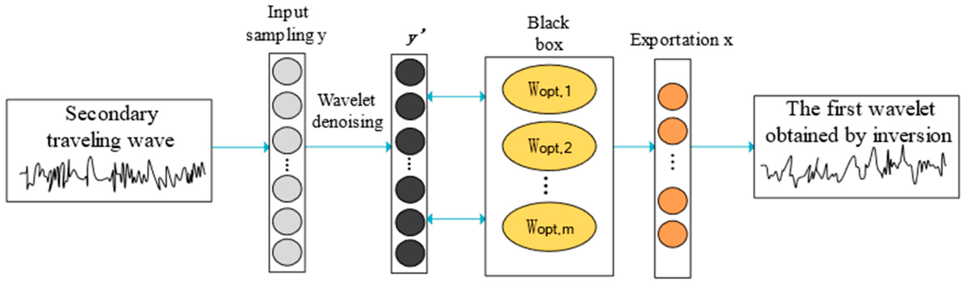
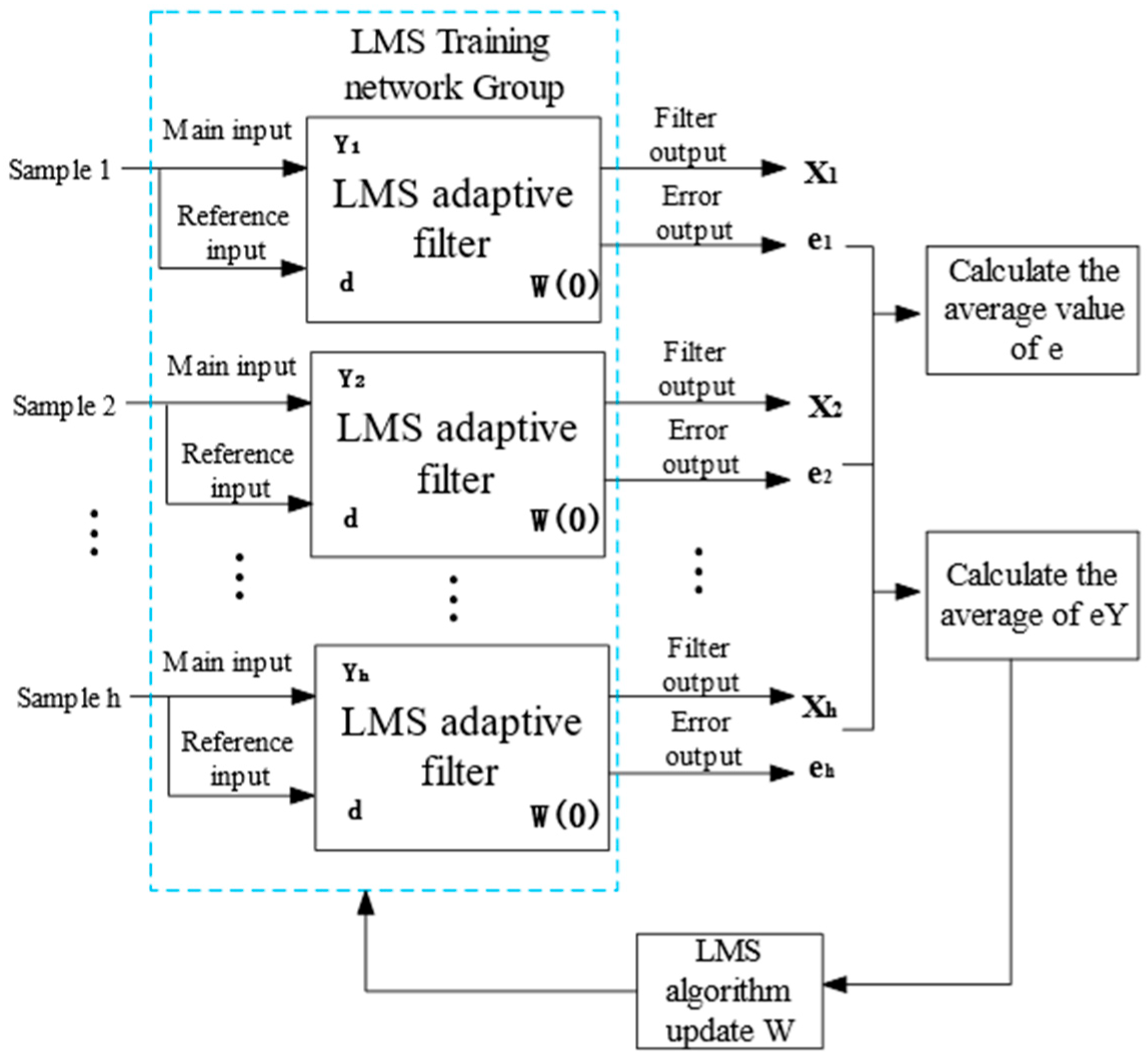
2.3. Wavelet Denoising

To solve the problem that the transient signal distorts in the process of transmission and cannot reflect the characteristics of the original waveform of the primary side traveling wave, an optimized variable step size Least Mean Squares (LMS) adaptive filtering algorithm is introduced in this study to achieve accurate detection of the transient waveform.

The process of wavelet threshold denoising is shown in Figure 1. By using an adaptive filter to learn and obtain the black box model parameter matrix A, the black box model is constructed.

The inversion process is shown in Figure 2. In the figure, y’ is the secondary signal after preprocessing and $W_{opt}$ is the best weight at time m. The schematic diagram of the adaptive filter is shown in Figure 3.

In the application of the LMS adaptive filter, a complete signal sequence $Y_{m+N}$ is introduced as the input signal, and an expected signal $d_m$ is set as the reference. At a given time $i$, the filter precisely extracts a specified interval $Y_i$ from the input signal, which is defined as the receptive field region. Then, the matched weight vector $W_i\left(n\right)$ obtained during the nth time iteration is used to weight the signal in the receptive field region, and the output signal $x_i\left(n\right)$ is estimated:

$$x_i(n)=\sum ^N y_{i-k+1}{w}_{i,k}=Y_i{(W_i(n))}^{\mathrm{T}}$$

(8)

where $y_{i-k+1}$ is the $k$ value of the $Y_i$ interval at the $i$ time; $w_{i,k}$ is the $k$ value in $W_i\left(n\right)$ at time $i$; and $n$ is the number of filter taps.

The error value $e_i\left(n\right)$ at time $i$ is the difference between the expected signal $d_i$ and the estimated signal at time $i$, as shown below.

$$e_i\left(n\right)=d_i-x_i\left(n\right)$$

(9)

In the input signal processing at subsequent time points, the signal in the current receptive field interval will be synchronously compared with the receptive field interval signal defined at the $i$ time; this process adopts the sliding window mechanism, in which the window definition length is a specific value. The weight vector update formula of the $n$ iteration is as follows:

$$W_i(n+1)=W_i\left(n\right)+2\mu e_i\left(n\right)Y_i$$

(10)

where $\mu$ is the step factor of the LMS algorithm, which determines the convergence speed and stability of the algorithm.

The weight vector is updated by using the update rule of the LMS algorithm, and the optimal weight vector $W_{opt}$ is obtained until the error signal is no longer reduced, so that the output of the filter is as close as possible to the expected signal.

The advantages of wavelet denoising

(1) Multi-scale analysis: By decomposing sub-bands of different frequencies, noise and signals are precisely separated.

(2) Localization feature: It can simultaneously locate noise in both the time domain and the frequency domain, making it suitable for handling non-stationary signals.

(3) Detail retention: Avoids edge blurring or excessive smoothing caused by traditional filtering methods.

(4) Flexibility and controllability: The effect can be optimized by choosing wavelet basis functions, the number of decomposition layers, and threshold strategies.

(5) Low computing cost: Compared with deep learning, it is suitable for embedded systems or real-time processing.

2.4. Model Construction

The single-phase grounding detection model based on PSO-SVM is mainly divided into two parts, the PSO algorithm and the SVM. By improving the inertia weight value in the particle swarm algorithm, the value of the learning factors is accordingly enhanced. Furthermore, by introducing a flight-time factor to optimize the particle position update formula, the optimization speed is accelerated, thereby obtaining an improved PSO algorithm. The SVM parameters C and g are fine-tuned using the improved PSO algorithm to find the most suitable parameters. After preprocessing the data set of grounding faults in low-voltage systems, it is divided into a training set and a test set in a certain proportion. The features of the data set are used as inputs, and the fault detection model is employed for prediction to obtain the output results. The specific steps of Figure 4 are as follows:

(1) Initialize the required parameters in the particle swarm optimization algorithm, including particle swarm size, maximum iteration count, learning factor, etc.

(2) Update the velocity and position of particle according to Equation (5).

(3) By using the pre-set fitness function, the fitness values of the particles appearing in the population are calculated.

(4) Compare the calculated particle fitness value with the best value found in history. If it is better than the historical value, replace it, otherwise it remains unchanged.

(5) Update inertia weights. Update the current inertia weight value based on the formula proposed in the previous text for improving weights.

(6) When the particles iterate to the predetermined maximum number of iterations, output the best solution found by the particles during the iteration process and output it. If the set number of iterations is not reached, return to step two and iterate again.

(7) Apply the optimized parameters (C and g) to the fault detection model.

(8) Apply the data set to the improved new model for training and testing.

2.5. True Experimental Data Processing

(1) Obtain raw current data.

The original grounding current data can be obtained by simulating the normal state of the low-voltage distribution area and different grounding fault types through the grounding test platform and simulation model in the low-voltage distribution area (because the protective resistance of the metallic grounding in the low-voltage distribution area is small, it is dangerous to obtain the original grounding data by means of the simulation model). However, there are redundant data and a lot of noise and harmonics in this data, so a series of data preprocessing operations are needed.

(2) Remove void data and reference values.

During the grounding experiment, adding the DC component to the test circuit can prevent the diode from burning out and ensure that the conditioning circuit is not reversed, but it will also cause the measurement baseline value of the current transformer to increase. Therefore, in order to ensure the accuracy of the total residual current detection, it is necessary to cut off the load, collect the DC data in the no-load line, and calibrate the current transformer. Take an average of all no-load data and subtract that average from all current data to eliminate the baseline value of the conditioning circuit, resulting in accurate total residual current data.

(3) Proportional reduction.

Due to the parameter setting of the conditioning circuit design in this experiment platform, there is a certain multiple difference between the collected data and the real data, because, in order to obtain the most authentic grounding data, the data need proportional restoration processing.

(4) Filter denoising

Due to the influence of the experimental environment and other aspects, the original grounding data collected by the NI equipment have great noise, so the original grounding data need to be denoised and filtered. The data waveform before and after processing is shown in Figure 5. It can be seen that the grounding waveform after wavelet transform filtering is smoother. With the decrease in the signal-to-noise ratio, the denoising effect slightly reduces.

3. Single-Phase Grounding Fault Testbed

3.1. Simulation Platform

This single-phase grounding fault occurs in a three-phase five-wire distribution system (L₁/L₂/L₃ phases, PEN protective neutral line, and PE dedicated protective earth, as shown in Figure 6). When a phase conductor (e.g., L₃) accidentally contacts equipment housing due to insulation failure, fault current I_d forms a loop through:

The single-phase grounding fault current originates at the fault point, passes through the contact resistance R_jc of the equipment housing, flows through either of the parallel local grounding devices (R_jd1/R_jd2), reaches the system’s main grounding resistance R_E to complete the circuit, and finally returns to the power neutral.

The single-phase grounding fault in this system will result in the following consequences: the generated residual current ranges from 30 mA to several amperes, potentially activating residual current protective devices to interrupt power supply. Additionally, elevated potential near the fault location creates electric shock hazards. Prolonged fault conditions may cause equipment overheating due to sustained fault current flowing through grounding resistances, leading to insulation degradation or equipment damage.

3.2. Experimental Platform

The experimental test platform for single-phase grounding faults in low-voltage distribution stations is shown in Figure 7. By testing the single-phase fault state and the normal operation state of the low-voltage distribution system, the data acquisition system collects the current data from the testbed.

4. Results

To perform cross-validation accuracy analysis of the model, the mode_selection module loads the cross_val_score function. Reusing data, cutting and dicing the collected sample data, combining them into distinct training and test sets, training the model using the training set, and assessing the accuracy of the model prediction using the test set are all examples of cross-validation. The accuracy distribution of the grounding fault detection model obtained after 20 cross validations is shown in Figure 8.

As can be observed from the above Figure, the average grounding fault detection accuracy is 99.69%, and the fault detection accuracy of the partial swarm optimization support vector machine (PSO-SVM)-based fault detection model can achieve over 99.5% in all multiple cross-validation scenarios.

The test set is used to evaluate the fault detection model based on PSO-SVM’s classification ability. The corresponding evaluation value of 99.9% is the output, and this evaluation value serves as the model classification ability evaluation index. It shows that the fault detection model based on PSO-SVM has qualified ability. Take the test set as the model’s input, evaluate the output, and then use the predict function to determine the relevant category (normal operation label: “0” and fault status label: “1”).

Tens of thousands of data sets are chosen as the effective data samples of the test set to conduct a number of in-depth tests on the fault detection model that has been constructed in order to demonstrate the reliability of the PSO-SVM-based fault detection model established in this paper.

Tens of thousands of experimental data that do not intersect with the training data samples are chosen in order to achieve this. After this, the data are jumbled to incorporate interference samples. In both the normal and grounding fault states, the load-shedding switches are activated in the branch circuit adjacent to the fault.

The confusion matrix algorithm model uses the two-dimensional matrix made up of test set labels and model test set output labels as input, and Figure 9 displays the confusion matrix’s schematic as output. The confusion matrix indicates that the fault detection model’s incorrect identification rate is 19 times, with the fault state being identified as the normal state 19 times and the normal state being identified as the fault state 0 times. The fault detection model’s detection accuracy, which is based on PSO-SVM, is 99.7%. In order to further improve the adaptability of the model under complex multi-operating conditions, it is necessary to further optimize the parameter configuration strategy and focus on exploring the influence mechanism of step size adjustment on system robustness. These will be the technical difficulties that need to be broken through in the subsequent algorithm iteration.

The conventional PSO technique uses a defined step size to update the particle position, which has a sluggish convergence speed, and a fixed inertia weight factor, which is simple to trap in the local optimum, has low solution accuracy, and has a low failure rate for fault detection. This work aims to increase the particle algorithm’s inertia weight value while simultaneously speeding up the optimization search speed and optimizing the particle location updating formula by adding the time-of-flight element. It is evident that, by comparing the SVM algorithm, the conventional PSO-SVM algorithm, and the enhanced PSO-SVM algorithm, the suggested approach in this study outperforms the conventional approach in terms of convergence speed and detection success rate. The specific results are shown in

Table 2. Performance Comparison.

	Detection Accuracy	Convergence Rate (ms)
PSO		25.5
SVM	85.6%	15.1
The traditional PSO-SVM	92.3%	211
The improved PSO-SVM	99.7%	156
WT	80.0%	-
STFT	75.0%	-
HHT	85.7%	-

.

5. Conclusions

A new single-phase grounding fault detection model based on PSO-SVM has been proposed in this research. The value of the learning factors is correspondingly increased by increasing the particle swarm algorithm’s inertia weight value. Additionally, the optimization speed is expedited by adding a flight-time element to the particle position update formula, which results in an enhanced PSO algorithm. To determine the best parameters, the enhanced PSO algorithm is used to fine-tune the SVM parameters C and g. Based on the improved PSO-SVM fault detection model, the fault detection accuracy of the simulation and experiment is up to 99.7%, indicating that the proposed method has high reliability.

References

1. Ye, Y.; Wang, S.; Huang, T.; Wei, L. Study on Grounding Mode of Neutral Point through Arc Suppression Coil in Parallel with Median Resistance. J. Electr. Eng. 2021, 16, 159–165. [Google Scholar]
2. Tian, P.; Qin, H.; Naiqian, H.; Qiang, Z. Fault Location Method for Distribution Network Based on Edge Computing and Wide Area Synchronous Measurement Technology. J. Electr. Eng. 2020, 15, 83–88. [Google Scholar]
3. Ye, B.; Xue, C.; Zhang, H.; Han, Y.; Liu, B. Research on fault line selection in distribution network based on feature band wavelet packet analysis. J. Electr. Eng. 2018, 13, 24–28. [Google Scholar]
4. Liu, Y.; Zhang, X.; Lv, Z.; Xu, Z.; Liu, Y. Research on intelligent diagnosis and route selection method of multi-load circuit series fault arc. J. Electr. Eng. 2023, 18, 378–388. [Google Scholar]
5. Li, W.; Xu, W.; Wang, X.; Lu, G. Fault location method for active distribution network based on generalized S transform. Electr. Meas. Instrum. 2021, 58, 105–112. [Google Scholar]
6. Yang, W.; Zhang, B.; Ye, X.; Zhao, Q. Sensor fault detection method in distribution network based on energy balance. Autom. Electr. Power Syst. 2018, 42, 154–159. [Google Scholar]
7. Li, Z.; Liu, Y.; Yan, Y.; Wang, P.; Jiang, X. An identification method for asymmetric faults with line breaks based on low-voltage side data in distribution networks. IEEE Trans. Power Deliv. 2021, 36, 3629–3639. [Google Scholar]
8. Liu, B.; Wang, C.; Zeng, X.; Wan, Z. Single line-to-ground fault protection method considering three phase-to-ground parameters asymmetry in active flexible grounding systems. IEEE Trans. Power Deliv. 2024, 39, 2207–2218. [Google Scholar] [CrossRef]
9. Liu, J.; Tai, N.; Fan, C.; Chen, S. A Hybrid Current-limiting Circuit for DC Line Fault in Multi-terminal VSC-HVDC System. IEEE Trans. Ind. Electron. 2017, 64, 5595–5607. [Google Scholar] [CrossRef]
10. Ali, M.S.; Abu Bakar, A.H.; Mokhlis, H.; Arof, H.; Azil Illias, H. High-impedance fault location using matching technique and wavelet transform for underground cable distribution network. IEEJ Trans. Electr. Electron. Eng. 2014, 9, 176–182. [Google Scholar] [CrossRef]
11. Liu, P.; Du, S.; Sun, K.; Zhu, J.; Xie, D.; Liu, Y. Single-line-to-ground fault feeder selection considering device polarity reverse installation in resonant grounding system. IEEE Trans. Power Deliv. 2021, 36, 2204–2212. [Google Scholar] [CrossRef]
12. Xue, Y.; Li, J.; Xu, B. Transient equivalent circuit and transient analysis of single-phase earth fault in arc suppression coil grounded system. Proc. CSEE 2015, 35, 5703–5714. [Google Scholar]
13. Yang, F.; Zhang, X.; Wang, Z.; Chen, S. Over-current protection of micro-grid with distributed generators. J. Shanghai Dianji Univ. 2015, 18, 89–94. [Google Scholar]
14. Lv, X.; Yuan, L.; Zuo, L.; He, Y.; Ding, C. An improved Bayesian learning method for distribution grid fault location and meter deployment optimization. IEEE Trans. Instrum. Meas. 2024, 73, 3519910. [Google Scholar] [CrossRef]
15. Zhang, P.; Jin, M.; Liang, R.; Hou, M.; Peng, N.; Li, J. Faulty cable segment identification of low-resistance grounded active distributions via grounding wire current-based approach. IEEE Trans. Ind. Inform. 2024, 20, 7708–7718. [Google Scholar] [CrossRef]
16. Liu, S.; Liu, H.; Bi, T.; Yu, X.; Jiang, Y. Fault Detection of Distribution Network Considering High Impedance Faults. Power Syst. Technol. 2023, 47, 3438–3448. [Google Scholar]
17. Li, T.; Xu, B.; Xue, Y. High-impedance fault protection of distribution networks and its developments. Distrib. Util. 2018, 35, 2–6. [Google Scholar]
18. Han, W.; Xu, J.; Mu, G. The analysis of earth fault with high resistance to longitudinal distance protection. Shanxi Electr. Power 2017, 3, 22–25. [Google Scholar]
19. James, J.Q.; Hou, Y.; Lam, A.Y.; Li, V.O. Intelligent fault detection scheme for microgrids with wavelet-based deep neural networks. IEEE Trans. Smart Grid 2019, 10, 1694–1703. [Google Scholar]
20. Yang, S.; Wu, S.; Dai, C. A method to fast recognize short-circuit fault based on curvature of line current wave form. Power Syst. Technol. 2013, 37, 551–556. [Google Scholar]
21. Sidhu, T.S.; Xu, Z. Detection of incipient faults in distribution underground cables. IEEE Trans. Power Deliv. 2010, 25, 1363–1371. [Google Scholar] [CrossRef]
22. Salim, R.H.; de Oliveira, K.R.C.; Filomena, A.D.; Resener, M.; Bretas, A.S. Hybrid fault diagnosis scheme implementation for power distribution systems automation. IEEE Trans. Power Deliv. 2008, 23, 1846–1856. [Google Scholar] [CrossRef]
23. He, Z.; Cai, Y.; Qian, Q. A study of wavelet entropy theory and its application in electric power system fault detection. Proc. CSEE 2005, 25, 38–43. [Google Scholar]
Figure 1. Process of wavelet denoising.
Algorithms 18 00259 g001
Figure 2. Inversion process.
Algorithms 18 00259 g002
Figure 3. Inversion of LMS adaptive training model flow with multiple samples.
Algorithms 18 00259 g003
Figure 4. Flowchart for constructing a low-voltage system fault detection model based on improved PSO-optimized SVM.
Algorithms 18 00259 g004
Figure 5. Comparison of current waveform before and after filtering and denoising.
Algorithms 18 00259 g005
Figure 6. Simulation Model.
Algorithms 18 00259 g006
Figure 7. Experimental model.
Algorithms 18 00259 g007
Figure 8. Distribution of cross-validation accuracy.
Algorithms 18 00259 g008
Figure 9. Illustration of model confusion matrix.
Algorithms 18 00259 g009