Generation of Realistic Synthetic Load Profile Based on the Markov Chains Theory: Methodology and Case Studies

Abstract

Digital energy systems rely on actual data about power consumption and generation, which are not always available and, in certain situations, can be replaced with synthetic forms. This study presents a methodology for generating synthetic time-series data of electrical power consumers. It is based on the Markov chains theory, and unlike previous studies, the data are divided into hourly and hour-change monthly records, which leads to the generation of 48 transition matrices for each month. This study aimed to ensure statistical and probabilistic similarity between the original and synthetic data, which was assessed using the Frobenius distance, the coefficient of determination, variance, and standard deviation. The methodology was applied to three load profiles obtained from different types of consumers—domestic, agricultural, and industrial. In all three cases, the statistical and probabilistic characteristics of the generated data were very similar to those of the original datasets; however, the visual comparison showed that it is recommended to increase the number of states to lower the data scattering. Based on the results, recommendations are proposed on choosing the number of states for the transition matrices to optimize the statistical and probabilistic similarity. The described methodology can be used by experts involved in the design of systems with renewable energy sources and by scientists dealing with long-term studies.

1. Introduction

The increasing integration of renewable energy sources into the modern power grids has highlighted the need for accurate and reliable energy load profiles. These profiles are crucial for grid management, energy forecasting, and optimizing demand–response strategies. However, obtaining real-world load data is often challenging due to privacy concerns, measurement limitations, and data availability [1]. As a result, a growing interest in developing synthetic load profiles that can mimic the statistical characteristics and probabilistic variations of actual consumption patterns is observed [2]. Solutions for creating models to generate synthetic data [3] are widely discussed in the literature [4,5,6].

Load profiles have the following features: they are data that reflect events or quantities over time and, therefore, carry a timestamp; they are a series of ordered pairs of values or states at a certain point in time, which are commonly fixed. Another characteristic of this series is that it is usually subject to certain time correlations and regular characteristics—there is some periodicity, trends, or seasonality. The characteristics can be extracted, processed, analyzed, and used to generate synthetic load profiles using various approaches and algorithms for time series analysis, signal processing, or machine learning (ML). In [7], 417 synthetic data generation models from the last decade are reviewed, and their functionalities and improvements are described. According to the authors, there is a trend towards increased performance and complexity of models, with neural-network-based models dominating. When a model is chosen, it is important to take into account that it is not possible to use the same approaches to synthetic data generation for different subject areas and that the time and cost of training ML algorithms should not be neglected. Systematic reviews of the application of machine learning models to synthetic data generation were also conducted in [8,9]. They cover synthetic data generation for application in various subject areas (computer vision, natural language processing, speech, different business aspects, healthcare, and others) and identify the challenges and opportunities of ML in data generation.

Long-term energy system analysis has been the subject of extensive research, primarily aimed at estimating future energy demand to guide the development of appropriate energy generation and distribution infrastructure [4]. With the advent of renewable energy, the forecasting requirement has also changed. Even in long-term applications, the time step has been reduced to reflect the rapid changes in production in short-term intervals. This change has led to the development of hybrid forecasting models that combine long-term planning with high-resolution temporal data to improve system flexibility and reliability. Due to these dynamics, using naturally collected data is sometimes insufficient, and it is often necessary to add synthetically generated data [10]. Another reason for this is the lack of high temporal resolution in the data (to accumulate real data, monitoring over a very long period is necessary) for electricity consumption, which makes it difficult to generate cost-effective, realistic forecasts and optimize the consumption. Furthermore, often privacy issues arise with the data used, which might be overcome by relying on synthetic data instead [11].

When it comes to data generation, the terms data forecasting and synthetic data generation are similar yet different. Forecasting is aimed at generating data that are as close as possible to the actual data, which has not yet occurred. Depending on the usage scenarios, the forecasts are commonly divided into very short-, short-, medium-, and long-term [12]. Considering the above, it is implemented on a probabilistic basis, i.e., algorithms are used to determine the scenario that has the highest occurrence probability.

Synthetic data generation could also be divided within the above-mentioned categories, depending on the specific application; however, in this case, the generated data must correspond to the real one only in a statistical and/or probabilistic way [13]. The synthetic data relies on random generators, i.e., these algorithms will not always “choose” the scenario with the highest probability of occurrence, unlike the forecasting ones.

ML algorithms are commonly used to extract information and knowledge from big data, but they can also be used to generate synthetic data for reasons, such as insufficient volume, gaps, availability, or confidentiality issues. In [14], the authors propose an approach for generating synthetic data for classification and regression that uses the K-nearest neighbor (KNN) model. The general framework of this approach includes the following main steps: from the available data, processed samples are prepared, which are used to train a KNN model to capture the correlations between the features.

ML algorithms have one major advantage in generating synthetic data—they can identify complex dependencies in the data and produce synthetic data sets that preserve the underlying statistical relationships and distributional characteristics of the original dataset. According to [15], the most popular ML approaches are generative adversarial networks (GANs), variational autoencoders (VAEs), and large language models (LLMs).

VAEs use a probabilistic approach to generate synthetic data. Unlike traditional autoencoders, VAEs introduce a stochastic component by encoding data into a distribution rather than a fixed point, enabling the generation of diverse and realistic samples [16]. VAEs are particularly useful in domains where high-dimensional and structured data, such as images, time series, and text, should be synthesized. In synthetic data generation, VAEs can produce new samples that resemble real-world distributions [17], making them valuable for augmenting datasets, addressing class imbalances, and enhancing privacy in machine learning applications by generating data that do not directly correspond to real entities.

LLMs are powerful tools for generating synthetic data by leveraging their ability to learn and generalize from vast amounts of text. Those models can produce realistic, coherent, and contextually appropriate text. Their capacity to generate diverse samples helps mitigate biases, improve model robustness, and create training data for low-resource languages or specialized domains. Additionally, LLMs can be fine-tuned to generate synthetic data tailored to specific requirements, such as anonymized text for privacy-preserving applications or domain-specific problems [18]. LLMs show high efficiency in producing synthetic text data but require significant computational resources.

The analysis in [19] identifies thirteen methods applicable for generating synthetic energy time series, which vary in frequency of occurrence. According to the authors, Markov models, weighted random number generator (wRNG) methods, and GANs are used in more than half of the articles.

Although GANs were developed with the main idea of image processing and computer vision, many researchers have shown in their publications [20,21,22,23] that they are also successfully applicable in synthetic data generation for the energy sector. Various modifications of GANs are an effective method for generating synthetic energy data that preserve the characteristics of real data. This provides significant opportunities for protecting privacy, reducing data collection costs, and improving research in energy systems. In [24], the authors proposed a data-driven application of deep GANs. They do not use synthetic data generation through system dynamics modeling but are based on learning the conditional probability distribution of the underlying features. The evaluation of the synthetically generated data was based on measuring the maximum mean discrepancy between real and synthetic data sets and showed strong convergence.

In theory, classical machine and deep learning approaches are also applicable in forecasting models for data generation by applying them for long-term “prediction” based on the previously predicted data. For example, in [25], the power of a PV generator was forecasted using an artificial neural network (ANN) with measured solar irradiance for the last 3 and 6 days and one forecasted value. The study reported a total of 7% forecasting error. A similar approach was used in [26], where a hybrid ANN model was applied for forecasting the power output of a thin-film PV installation. The study achieved a relative root mean square error between 3.59% and 8.65%, depending on the solar radiation intensity. Even though the authors did not investigate the application of their models for generating synthetic data, they could be combined with a random generator for forecasting solar irradiation.

Another major approach to generating synthetic load profiles is the application of probabilistic models, particularly those based on experimentally obtained data. Among these, Markov chains and other ML techniques offer a robust mathematical framework for modeling and predicting energy consumption patterns while preserving key statistical and temporal properties. By leveraging historical data, synthetic load profiles can support simulation-based analysis, demand-side management, and the optimization of renewable energy systems. Markov chains are considered a less powerful apparatus than machine learning models, but they are a lighter and more efficient alternative recommended for usage with time series data [7].

In [27], the authors examined the generation of household electrical load schedules using Markov chains. Their main goal was to create synthetic electricity consumption schedules that reflect the actual electricity consumption patterns in different types of dwellings. A first-order Markov chain based on a 24 × 24 transition matrix was used to model the transition between different levels of electricity consumption. The analysis was based on consumption data collected at 30 min intervals over six months from five different types of dwellings in Ireland. The model successfully reproduced the basic statistical characteristics, such as mean and standard deviation. However, the synthetic profiles failed to capture the temporal structure of peaks and troughs in consumption.

Another study [28] aimed to find a method for generating synthetic energy production and consumption profiles that reflect the statistical and temporal characteristics of real data, focused on creating multiple scenarios that can be used for microgrid design and optimization. A Markov chain approach was proposed, based on historical data for electricity consumption, heat costs, and solar production. The approach combines clustering to reduce data and determine transition matrices for different periods (in this case, hourly intervals). The synthetic profiles successfully reproduced the main statistical characteristics of the real data, such as averages, seasonality, and time cycles. The approach shows flexibility, allowing both long-term forecasts for design and short-term forecasts for microgrid management.

A model for the synthetic generation of solar irradiation data using Markov chains and time segmentation was proposed in [29]. Solar irradiation is classified into four categories: low, medium, high, and very high, according to the intensity of solar radiation. The data are divided into time segments, and a separate transition matrix is calculated for each segment. The algorithm uses these matrices to generate synthetic values of irradiation for each time interval. Such an approach is applicable in the design of energy storage systems and optimization of smart grids; however, a calibration of the model to a specific geographical location is required.

An application of Markov models to predict future states based on user behavior and sensor data is described in [30]. The goal is to implement an intelligent decision support system based on reinforcement learning that analyzes user behavior and environment data to predict energy consumption. Although this approach shows potential for significant cost reduction and efficiency increase in managing energy consumption in the domestic sector, it also has some problematic aspects, such as difficulties in identifying similar behavior patterns between different days, as well as the need to improve the system to work in real conditions with more complex sensor data.

A stochastic model for managing electricity consumption that reflects the variability of consumers’ social activities is described in [31]. The model uses Markov chains with random transition matrices to model missing data. Consumers’ daily activities are classified into four basic states: “away”, “sleeping”, “home with high consumption”, and “home with low consumption”. The transition matrices are calculated from time-use data but include stochastic elements to fill in missing or limited data and aggregate the states. The maximum entropy approach is used to define the probabilities of the transition matrices.

In [29], it is shown that solar states are interdependent and, therefore, can be modeled with Markov chains. In particular, a multi-segment Markov chain was used, in which the transition probabilities from one solar state to another depended on the moment of time. To capture this dependence, the time intervals were divided into segments, and for each one, a transition matrix was defined based on real data. The study showed promising results; however, the number of states was not calibrated, and the relationship between the number of time segments and solar radiation was not investigated.

The analysis of the probability of different events occurring in the renewable sector with Markov chains has also been studied by various authors. In [32], it is shown that the probability for prolonged (10 days) periods of low energy output from photovoltaic installations in Ruse (Bulgaria) varies between 0% and 20% for the different months of the year. Another study for Mogilishte (Bulgaria) demonstrated that the probability of wind turbines’ power being below 20% of their rated value for 10 consecutive days varies between 0% and 70% for the different months of the year [33]. Such information could be of crucial importance when designing autonomous installations with renewable energy sources. It shows that the probabilistic information is as important as the statistical information for the energy sector.

The analysis of previous studies shows that two main approaches exist for synthetic data generation—the application of deep GANs and Markov chains. An obvious research gap is that the probabilistic characteristics of the data generation solutions were neither investigated nor optimized. However, when it comes to load profiles and digital energy systems, it is important to maintain the occurrence probabilities of different random events, such as extreme peaks, prolonged high or low consumption, etc. Therefore, the synthetic data for energy applications should keep both the statistical and probabilistic characteristics of the original time series, especially when renewable energy is involved.

This study aimed to develop a methodology for generating synthetic load profiles that retain the statistical and probabilistic characteristics of the actual experimental data. To achieve this, evaluation criteria and general application recommendations will be defined. The proposed approach will enable the generation of realistic energy demand profiles that reflect the actual consumption trends and the probabilities for the occurrence of different random events, which is the main contribution of this study. Furthermore, the paper includes several case studies to demonstrate the application of the methodology and to illustrate its potential applications in the field of energy management. By providing a scalable and statistically sound approach to synthetic load profile generation, this research aims to contribute to the advancement of data-driven energy system analysis, enabling improved demand forecasting, load balancing, and integration of distributed energy resources.

2. Materials and Methods

2.1. Basic Requirements

Before a methodology for the generation of a synthetic load profile is proposed, the requirements for it should be strictly defined. As previous studies have shown [32,33], both random processes and load profiles have not only statistical characteristics but also probabilistic ones, which can have a major impact on the reliability of decentralized and autonomous energy systems with energy storage. For example, the two load profiles in Figure 1 have the same statistical characteristics (the same distributions) as they contain the same samples, however, their probabilistic characteristics are different.

The one in Figure 1a crosses the level Lk = 2 kW six times (three times by a positive direction and three times by a negative direction), which indicates that if the current power is above 2 kW, there is a 12.5% probability that the next power will be below 2 kW. On the other hand, for the load profile presented in Figure 1b, this probability is only 4.2%.

The abovementioned allows us to define the requirements for the developed methodology. The generated synthetic load profile should conform to the following:

• The random generator should allow generating data with a time step of 15 min or less.
• The generated synthetic data should have an identical statistical distribution to the training data.
• The generated synthetic data should have identical probabilistic properties as the training data.

2.2. Methodology

Taking into account the defined requirements, a methodology for the generation of a synthetic load profile is proposed (Figure 2), which is based on the Markov chains theory. It contains four major steps, which are explained below.

Step 1. Data preparation

In this initial phase, the training data are acquired, which includes two phases:

Phase 1.1. Data collection—In this phase, a time series is obtained from an energy meter or other means, such as a photovoltaic system with a smart meter. While no strict requirements are defined for the number of samples, it is understandable that the higher the volume of data is, the clearer the image of the load will be. The used data should include the following columns:

• a timestamp, including the date and time of the measurement;
• instantaneous (or average) power of the load for the corresponding moment.

Phase 1.2. Data preprocessing—Next, the collected data are preprocessed, which includes several different aspects:

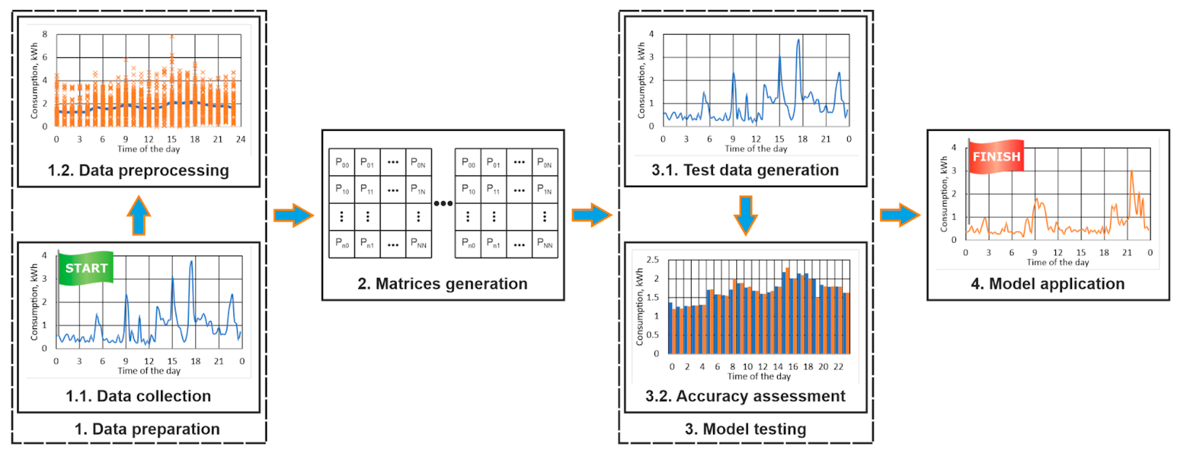
• The time series is verified for inconsistencies, which should either be excluded or corrected (if applicable). Such situations might include records with empty values, negative values, unrealistically high values, etc. This verification could be made either manually or using different tools and approaches, including statistical methods for outlier detection.
• If the time step of the series is lower than intended, it should be increased by choosing an appropriate approach. For example, if the time of discretization of the dataset is 5 min, and it should be analyzed in 15 min batches, then the data should be resampled. The new 15 min records could be formed either by selecting the corresponding records or by averaging them with the nearby records.
• The time series should be divided into appropriate batches, depending on its seasonality. For example, if the load profile characteristics are different for the different months of the year, then it should be analyzed independently for each month. In the current study, we have adopted this approach.

Step 2. Matrices generation

In this step, the transition matrices are generated, which include

-

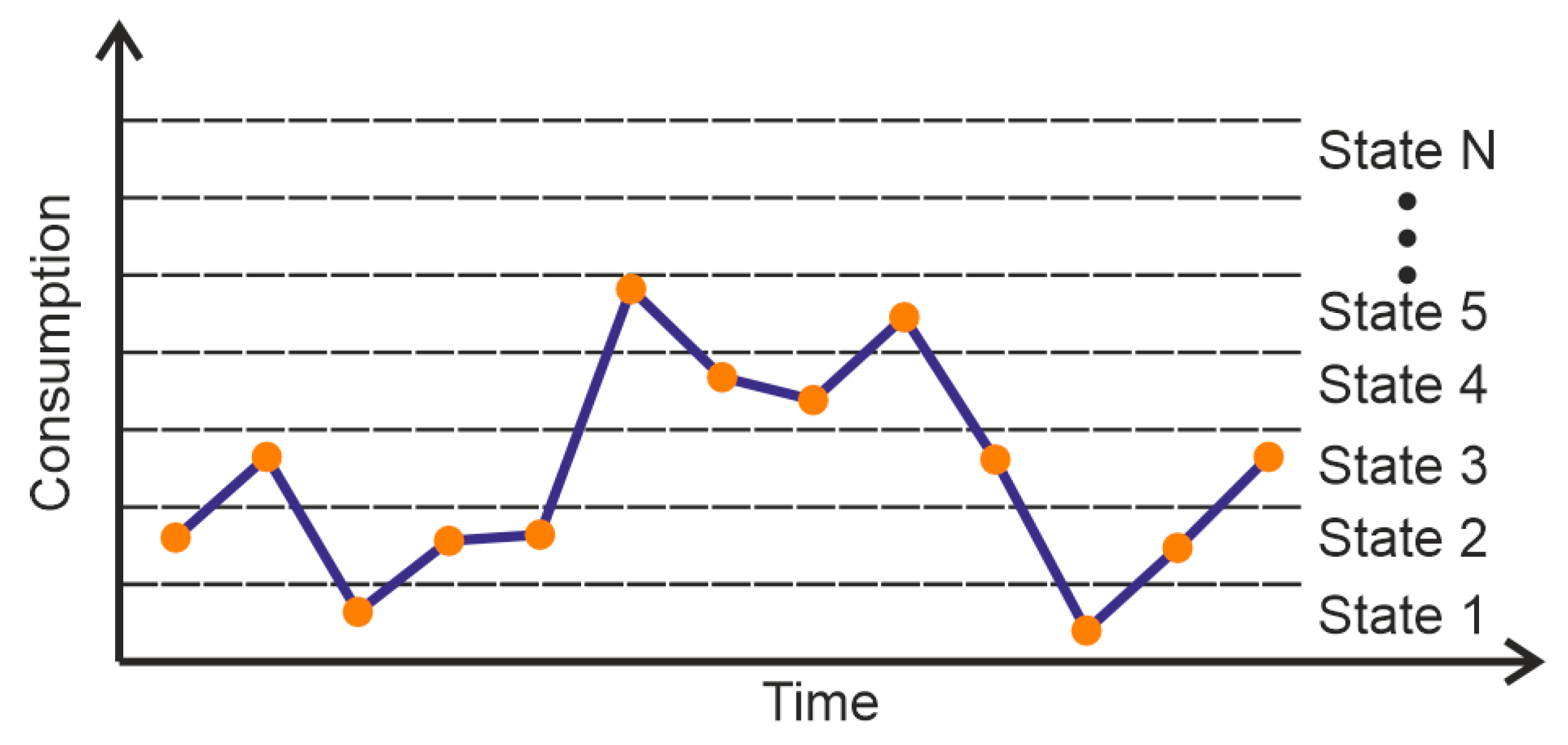
Choosing the number of states, i.e., the dimensionality of the matrices. The data are divided into N states (Figure 3) of equal width, which is estimated according to

$$StateWidth={\displaystyle \frac{P_{max}-P_{min}}{N+1}},W,$$

(1)

where P_max and P_min are the maximal and minimal power consumptions for the investigated time series.

-

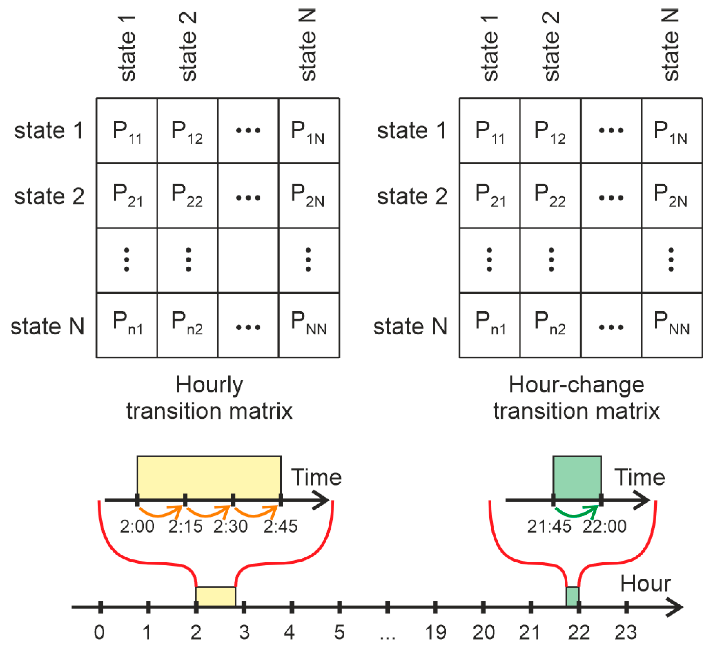
Generating 24 transition matrices for each hour of the day, based on the Markov chain theory. In other words, each discrete sample of the load profile data is classified into one of the N states and the probabilities of jumping from each state to all other states are estimated for each hour of the day (Figure 4). These matrices are generated using all pairs of sequential records, which belong to the same hour of the day (for example, if the time of discretization is 15 min, the records at 09:30 and 09:45 are consecutive and belong to the same hour).

-

Generating 24 transition matrices containing the probabilities for changing states when an hour is changed (Figure 4). They are based on all pairs of sequential records, which belong to different hours (for example, if the time of discretization is 15 min, the records at 9:45 and 10:00 belong to different hours of the day).

The following example is given for a better understanding of the difference between hourly and hour-change matrices. If there are five consecutive records, respectively, at 21:00, 21:15, 21:30, 21:45, and 22:00, the pairs (21:00 -> 21:15), (21:15 -> 21:30), and (21:30 -> 21:45) are used to generate the hourly transition matrix for the 21st hour. Similarly, the generation of the hour-change transition matrix between the 21st and the 22nd hours is based on the pair (21:45 -> 22:00).

Step 3. Model testing

The next step is to test the generated matrices to see whether they can be used to generate synthetic data with an acceptable accuracy. This step includes two phases:

Phase 3.1. Test data generation—a random generator is used to create synthetic data for a certain month of the year. This procedure includes the following:

• The initial hour and state for the data (for example, 0 h) are chosen—the chosen state must have non-zero probability in the corresponding hourly transition matrix;
• The next state of the synthetic data is generated randomly, according to the probability distribution for the current state in the transmission matrix, which could be achieved as shown in Algorithm 1.

Algorithm 1. Generating the next state according to the transition matrix probabilities.

Let Xt be the last state NumberOfTransitions = Count(Mh:h, Xt)//Get the total number of possible transitions (according to the original dataset) from the current state Xt RandomNumber = rand(1 … NumberOfTransitions)//get a random number between 1 and NumberOfTransitions NextState = 0//initialize while RandomNumber > 0 {   if RandomNumber <= Mh:h(Xt, NextState)//Mh:h(Xt, NextState) are the number of possible transitions from Xt to NextState   {     Xt+1 = NextState;//the next state has been randomly generated     break;   }   RandomNumber = RandomNumber − Mh:h(Xt, NextState);   NextState = NextState + 1 }

• Once the new state S_t+1 is generated, the value of the next sample is estimated according to

  $$P_{t+1}=StateWidth\times \left(S_{t+1}-1\right)+random\left(0\dots StateWidth\right),$$

  (2)

  where random(0 …StateWidth) returns a random value between 0 and StateWidth. When the current and the next generated records belong to the same hour of the day, the corresponding hourly transition matrix is used; if they belong to different hours, the corresponding hour-change transition matrix is used.

When testing data are generated, the record count should be large enough, and often it might be larger than the training dataset. This is required to make sure the long-term trend of the Markov chain has reached its final probability distribution vector.

There is one situation that requires special handling: the final state of the previous hour X_t may exist in the hour-change transition matrix M_h:h+1 with zero probability. This can happen because of the limited volume of the training dataset, though it is also possible in very large training datasets. This situation is handled according to Algorithm 2. Initially, the algorithm tries to generate a new final state X_t from the previous state X_t−1, which has a non-zero probability in the hour-change transition matrix M_h:h+1. If it does not succeed N number of times, then the new state X_t+1 is chosen randomly from the hour-change transition matrix based on its probability distribution.

Algorithm 2. Handling of the situation where the current state exists in the hour-change matrix with a zero probability.

Let Xt be the last state for the hour h if the probability for the current state in the transition matrix Mh:h+1 (the matrix, describing the transition between the h hour and the h + 1 hour) is 0: {   repeat N times:   {     Xt = Mh:h(Xt−1)//Generate the last state Xt again (the transition between Xt−1 and Xt)       if the transition probability from state Xt in Mh:h+1 is nonzero:     {       //Continue with the newly obtained state Xt;       break;     }   } } if an appropriate state Xt was obtained, for which a transition exists in the matrix Mh:h+1: {   Xt+1 = Mh:h+1(Xt)//generate the next state Xt+1 from the current state Xt } else {   Xt+1 = rand(all states)//randomly choose a new state from all states in Mh:h+1. }

Phase 3.2. Accuracy assessment—This phase aims to compare the synthetic and training data in terms of distribution and probabilities to assess how closely the synthetic data represent the original one.

The following measures can be used to compare the synthetic and training data statistically:

• The standard deviation of the energy consumption:

$$\sigma =\sqrt{{\displaystyle \frac{1}{n-1}}\sum _{i=1}^n(x_i-\overline{x})}$$

(3)

• The variance of the energy consumption:

$${\sigma }^2={\displaystyle \frac{1}{n-1}}\sum _{i=1}^n(x_i-\overline{x})$$

(4)

To compare the original and synthetic load profiles probabilistically, their hourly and hour-change matrices should be compared. The matrices describing the synthetic data should be generated as described in phase 3.1 of the methodology. It should be noted that while it is expected that these matrices match perfectly, this is not always the case. As mentioned in phase 3.1, sometimes the final state for an hour does not exist in the next hour-change transition matrix, which leads to changes in the probabilities of the synthetic time series. The following metrics could be used for comparing two matrices A and B:

• the Frobenius distance:

$$F=\sqrt{\sum _{i=1}^n\sum _{j=1}^n{\left(a_{ij}-b_{ij}\right)}^2},$$

(5)

which returns a positive value or zero. It could be interpreted as follows: the closer F is to zero, the closer the two matrices are. It is an extension of the Euclidean distance for matrices and allows measuring the common difference between two matrices [34].

• the coefficient of determination (R²) [35]—in order to apply it on matrices, they should first be converted from n × n dimensional ones to an n² dimensional vector.

$$\begin{gathered} A_{\mathrm{n}\times \mathrm{n}}=\left[\begin{array}{ccc}{x}_{11}& \dots & x_{1n}\\ ⋮& \ddots & ⋮\\ x_{n1}& \dots & x_{nn}\end{array}\right] \to A_{{\mathrm{n}}^2\times 1}=\left[\begin{array}{cc}{x}_{11}& \dots \end{array} \begin{array}{cc}{x}_{1n}& \dots \end{array} \begin{array}{ccc}{x}_{n1}& \dots & x_{nn}\end{array}\right] \\ {B}_{\mathrm{n}\times \mathrm{n}}=\left[\begin{array}{ccc}{y}_{11}& \dots & y_{1n}\\ ⋮& \ddots & ⋮\\ y_{n1}& \dots & y_{nn}\end{array}\right] \to B_{{\mathrm{n}}^2\times 1}=\left[\begin{array}{cc}{y}_{11}& \dots \end{array} \begin{array}{cc}{y}_{1n}& \dots \end{array} \begin{array}{ccc}{y}_{n1}& \dots & y_{nn}\end{array}\right] \end{gathered}$$

(6)

Thereafter, the two one-dimensional vectors A_n² and B_n² can be compared with

$$R^2={\left[{\displaystyle \frac{n\times {\sum }_{i=1}^n\left(x_i\times y_i\right)-{\sum }_{i=1}^n\left(x_i\right)\times {\sum }_{i=1}^n\left(y_i\right)}{\sqrt{n\times {\sum }_{i=1}^n\left(x_i^2\right)-{\left({\sum }_{i=1}^n\left(x_i\right)\right)}^2}\times \sqrt{n\times {\sum }_{i=1}^n\left(y_i^2\right)-{\left({\sum }_{i=1}^n\left(y_i\right)\right)}^2}}}\right]}^2$$

(7)

R² is a statistical measure that determines the proportion of variance in the dependent variable that can be explained by the independent variable in a regression model. Values close to 1.0 would indicate that the matrix of the synthetic data is almost identical to the original one, while lower values indicate the two variables are more or less different [36].

According to the proposed methodology, the synthetic load generation model is represented by 24-hourly and 24 h-change transition matrices. Therefore, two average values are estimated, respectively, for the hourly and the hour-change matrices, which are used for deeper analysis.

Step 4. Model application

Once the Markov chain model has been tested and approved, it can be used to generate synthetic data for different simulation scenarios, such as the sustainability of rare events, risk analysis, etc.

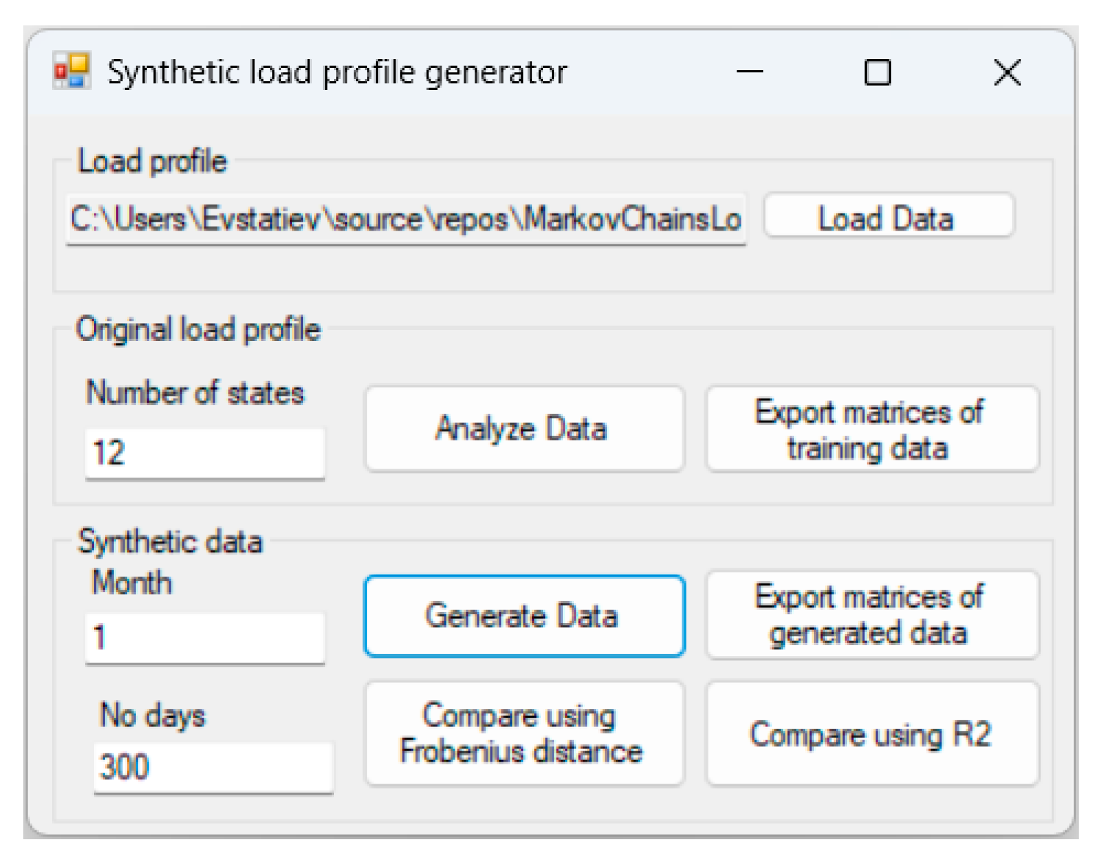
2.3. Means of the Investigation

The described methodology for generating a synthetic load profile and the methods for probabilistic analysis of the data were implemented in a specialized software tool developed in Microsoft Visual Studio 2019 (Figure 5).

It supports the following functions:

• The “Load Data” button loads the training dataset from a tab-delimited file containing the month of the year, the hour of the day, and the power consumption (

  Table 1. Sample training tab-delimited file containing a load profile.

  Month of the Year	Hour of the Day	Power, kW	Comment (Not Part of the File)
  11	17	2.4	Power consumption for 17:15
  11	17	2.48	Power consumption for 17:30
  11	17	2.28	Power consumption for 17:45
  11	18	1.6	Power consumption for 18:00

  ). The developed tool assumes that the data has a 15 min time step.

2.

The “Analyze Data” button estimates 24 hourly and 24 h-change transition matrices, based on the provided dataset and the defined number of states (in the “Number of states” field).

3.

The “Generate Data” button generates synthetic data for the defined number of days (in the “No days” field) and month (in the “Month” field) with a 15 min time step. The synthetic data are automatically exported in a tab-delimited file.

4.

The buttons “Export matrices of training data” and “Export matrices of generated data” export the hourly and hour-change transition matrices of the training and synthetic datasets, respectively.

5.

The button “Compare using Frobenius distance” estimates the Frobenius distances between each two corresponding matrices of the original and generated datasets and exports them in a tab-delimited file.

6.

The button “Compare using R2” estimates the R² values between each two corresponding matrices of the original and generated datasets and exports them in a tab-delimited file.

The statistical analysis and the graphical representations of the data metrics and data fragments were implemented in Microsoft Excel 2021, v. 2108.

3. Results and Discussion

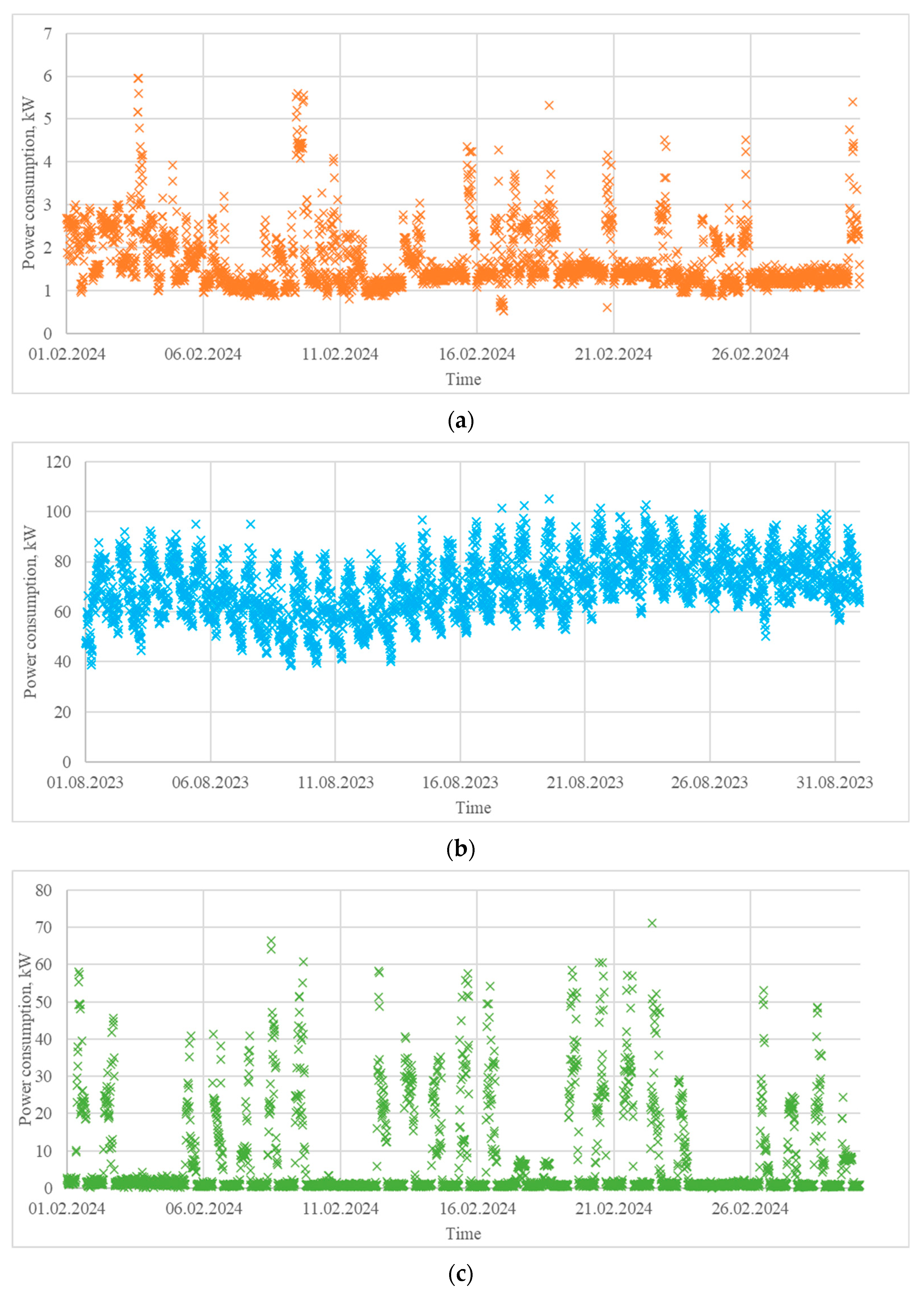
3.1. Testing Datasets

Three datasets were selected for testing the methodology, which are characterized by different statistical and probabilistic characteristics:

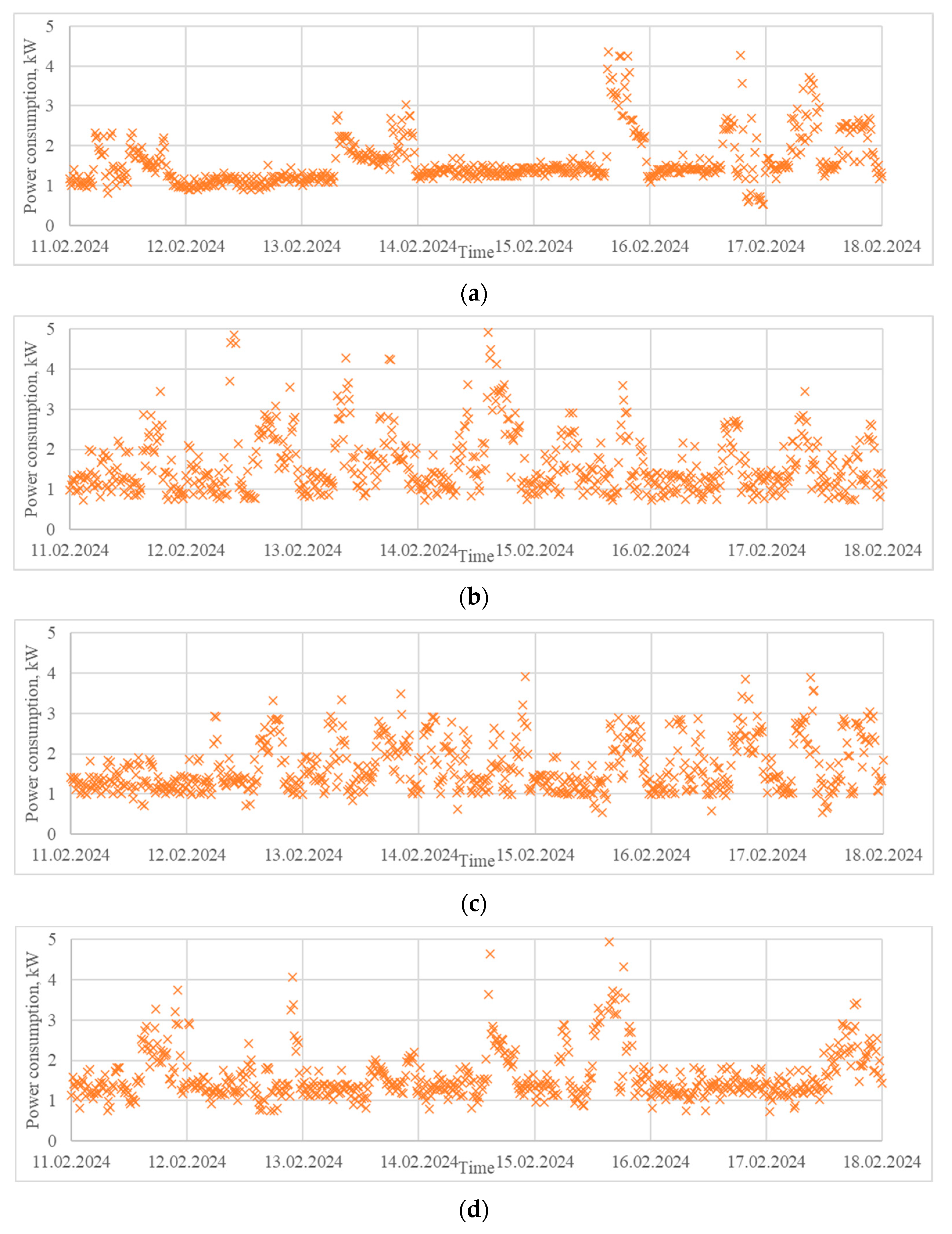
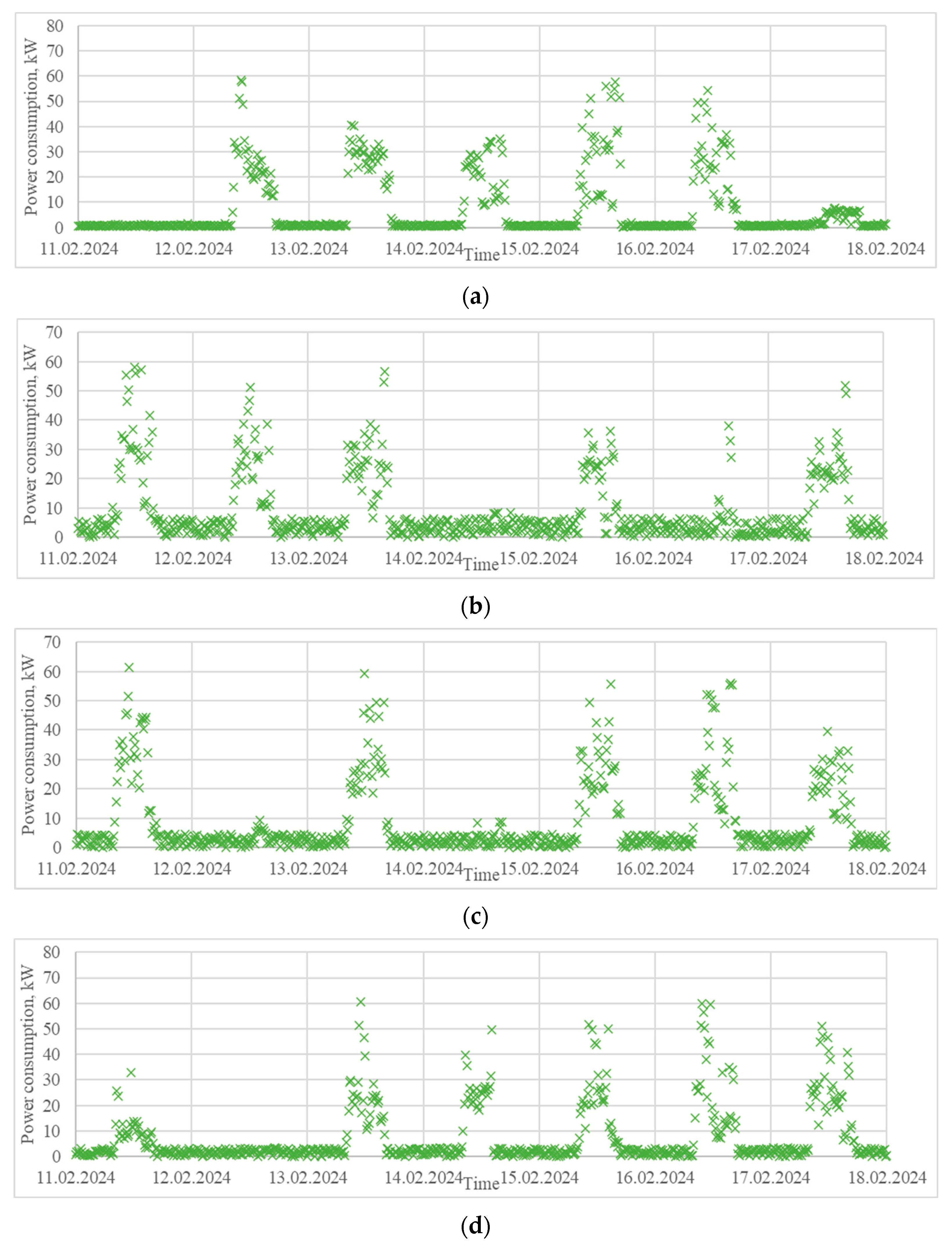
• A load profile extracted from a house located in the region of Ruse, Bulgaria, in the period 1–29 February 2024 (Figure 6a). It is characterized by power consumption varying in a wide range and significant peaks during the weekends. Residential load profiles are generally influenced by many factors, such as the type of day (weekday or weekend), hour of the day, meteorological conditions, people’s lifestyle, holidays, etc.
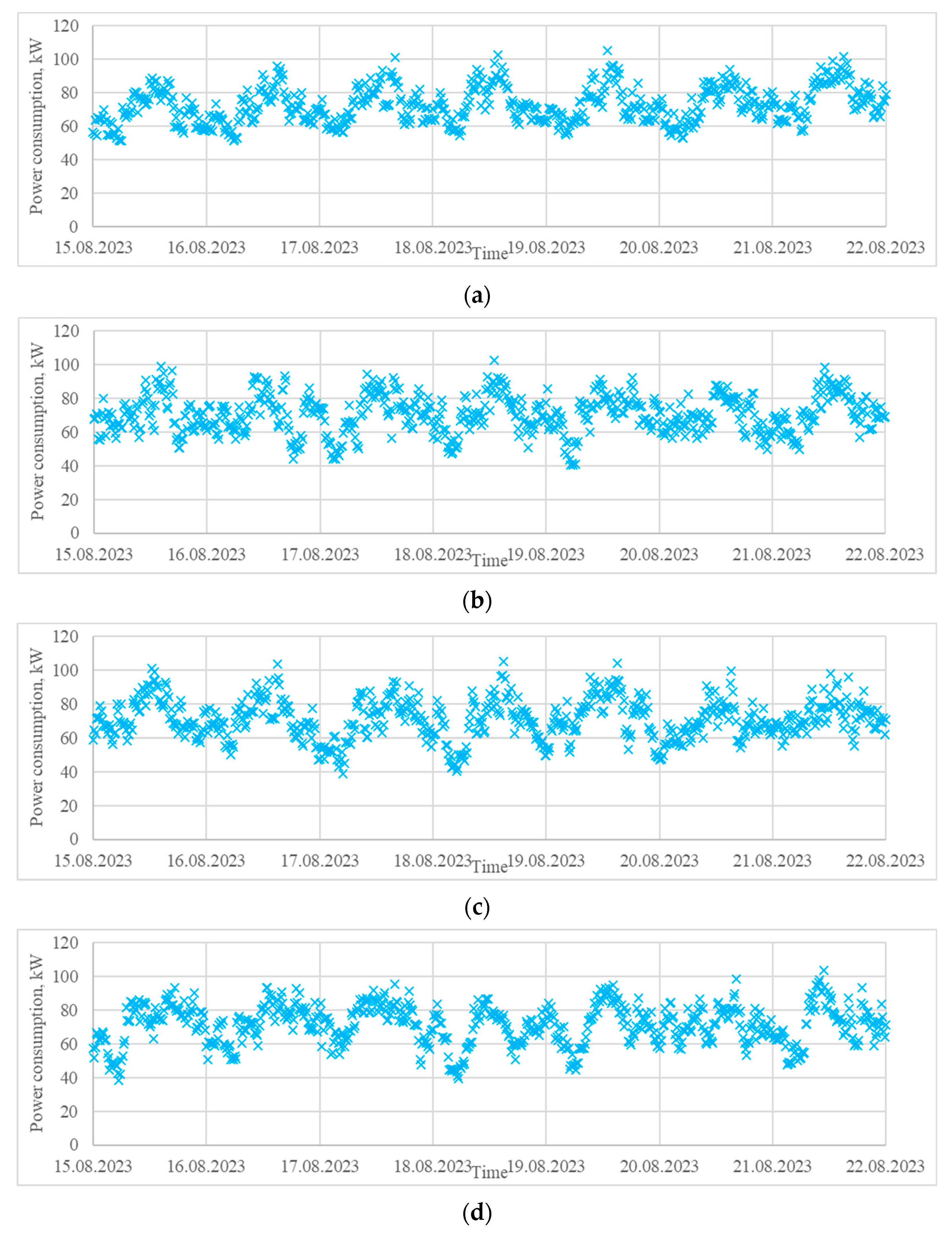
• A load profile of a pig farm located in the region of Silistra, Bulgaria, in the period 1–31 August 2023 (Figure 6b). It is characterized by relatively similar daily variations, which can be explained by the agrotechnological requirements. Load profiles in livestock farming are influenced mostly by the schedule of the technological processes (lighting, feeding, ventilation, etc.) and the meteorological conditions.
• A load profile of a printing house, located in the region of Varna, Bulgaria, for the period 1–29 February 2024 (Figure 6c). It is characterized by significant electrical consumption during the working hours of the weekdays and almost zero consumption during the rest of the time. Industrial load profiles are greatly influenced by factors such as the type of day (weekday or weekend), hour of the day, daily schedule, holidays, and the meteorological conditions.

3.2. Comparison Between the Training and Synthetic Data

3.2.1. Case Study 1: Generation of Synthetic Power Consumption Data for a Domestic Consumer

As already stated, the investigated load profile of the domestic consumer is characterized by uneven consumption during the days, which can be explained by the lifestyle of the people living there.

To investigate the performance of the applied approach, the load profile was evaluated using a different number of states varying between 10 and 26. For each number of states:

• Matrices were generated according to Step 2 of the methodology.
• 10,000 days of synthetic data were generated according to Step 3.1 from the methodology to make sure the long-term trend of the generated data has reached the final probability distribution vector.
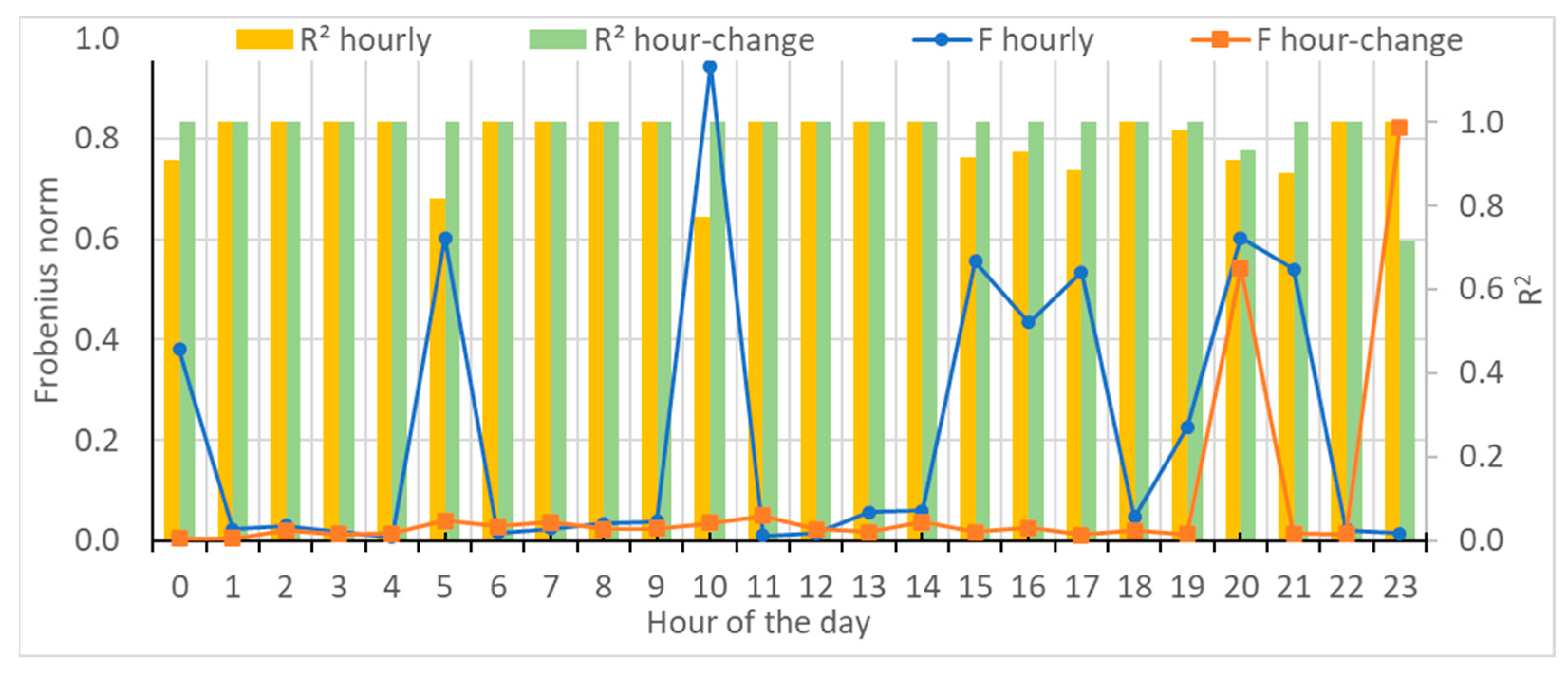
• The matrices of the synthetic and of the original data were compared using the Frobenius distance and R², according to Step 3.2 of the methodology.
• The average Frobenius distance and R² were estimated for each hour of the day.
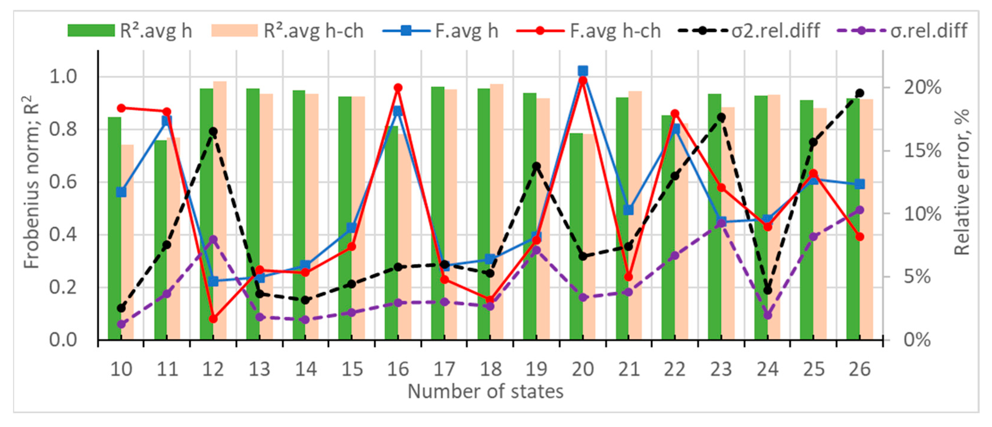
• The relative difference between the variance and standard deviation of the original and the synthetic data was obtained.

Initially, the Frobenius distances and the R² values were estimated for each hour of the day and each number of states. For example, Figure 7 presents the situation with 12 states.

Next, their average values were estimated for each number of states, with the results summarized in Figure 8. It can be seen that the average Frobenius distance of the hourly matrices varied between 0.22 and 1.03 and had a minimum at 12 states, as well as local minimums at 17 states and 23 states. Similarly, the average Frobenius distance for the hour-change varied between 0.08 and 0.99 and had a minimum at 12 states and local minimums at 18 states, 21 states, and 24 states. The average R² of the hourly matrices varied between 0.76 and 0.96 and had maximums at 12, 13, 17, and 18 states. Similarly, the average R² of the hour-change matrices varied between 0.74 and 0.98 and had a maximum at 12 states and local maximums at 18 and 24 states.

Regarding the statistical analysis, it can be observed that the relative error of the variance varied between 2.54% and 19.59% and had a minimum at 10 states. The errors remained below 6% between 13 and 18 states, as well as at 24 states. Similarly, the relative error of the standard deviation varied between 1.28% and 10.33%. It had a minimum of 10 states and local minimums of 14, 18, 20, and 24 states.

A good candidate in terms of the number of states is expected to have low Frobenius distances, low variances, and low standard deviations, as well as R²s near 1. Since there is no perfect combination, the following situations were investigated more closely (

Table 2. Comparison between the metrics of the three generated datasets of the domestic consumer with 12, 18, and 24 states.

Metric	Synthetic Data with 12 States	Synthetic Data for 18 States	Synthetic Data for 24 States
Average Frobenius distance of the hourly matrices (F.avg h)	0.22	0.31	0.46
Average Frobenius distance of the hour-change matrices (F.avg h-ch)	0.08	0.15	0.43
Average R2 of the hourly matrices (R2.avg h)	0.96	0.96	0.93
Average R2 of the hour-change matrices (R2.avg h-ch)	0.98	0.97	0.93
Relative error of the variance (σ2.rel.diff)	16.55%	5.26%	3.94%
Relative error of the standard deviation (σ.rel.diff)	7.96%	2.67%	1.99%

):

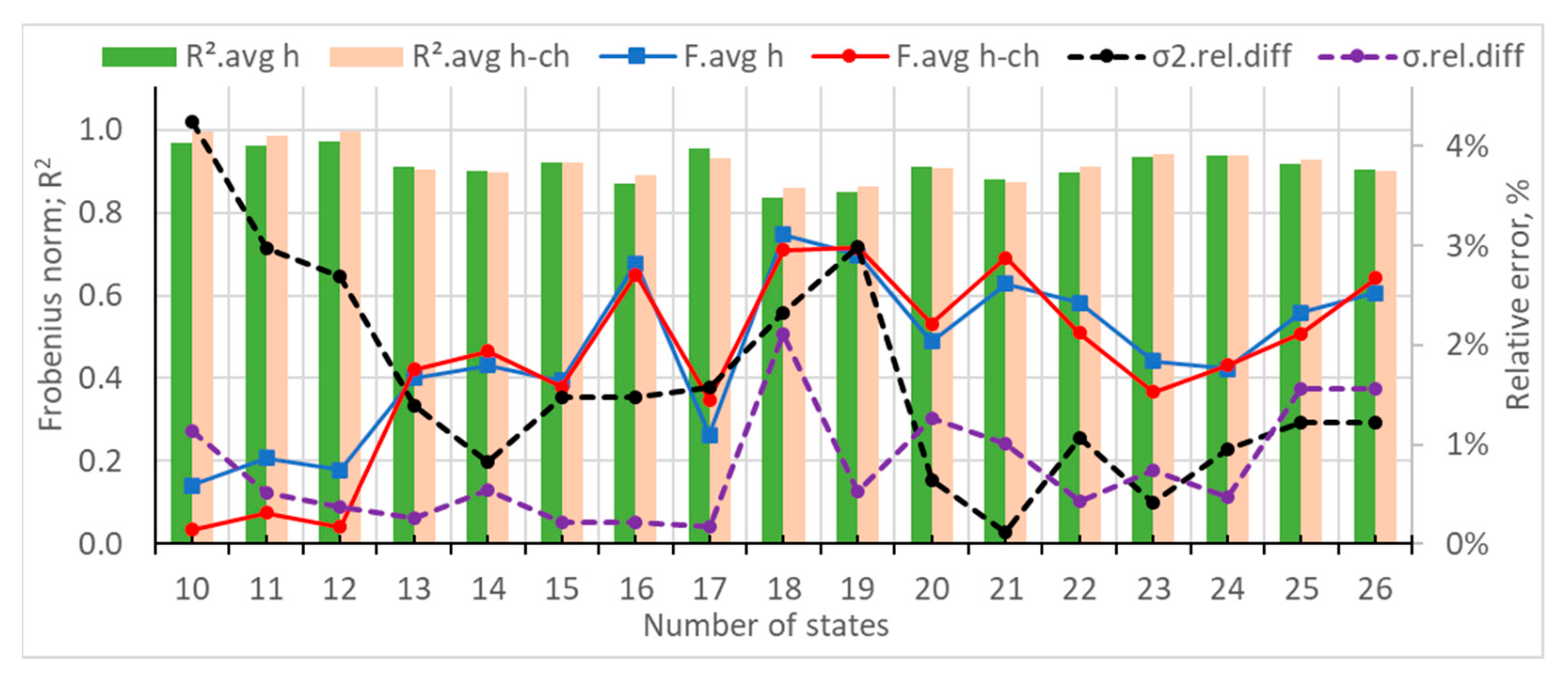
• The generated data with 12 states, which was characterized by the lowest Frobenius distances and the highest R² values, but with higher relative error for the variance and standard deviation.
• The generated data with 18 states, which was characterized by a local minimum of the Frobenius distances, high R² values, and local minimums of the statistical measures.
• The generated data with 24 states, which was characterized by local minimums of the Frobenius distances and the statistical measures, as well as high R² values.

It can be seen that the data of the domestic consumer generated with a higher number of states had better statistical metrics, but slightly worse probabilistic ones; i.e., the choice of an optimal solution is a tradeoff between them. To better understand these three situations, 7 days of data were generated (Step 4 from the methodology), respectively, with 12 (Figure 9b), 18 states (Figure 9c), and 24 states (Figure 9d) and visually compared with 7 days from the original dataset (Figure 9a). It can be visually observed that the data generated with fewer states was more scattered compared to synthetic data with more states. This can be explained by the wider width of each state and the fact that once a state is generated, the exact value is synthesized using a uniform distribution. Therefore, when the evaluation metrics are similar, the scenario with the higher number of states should be selected.

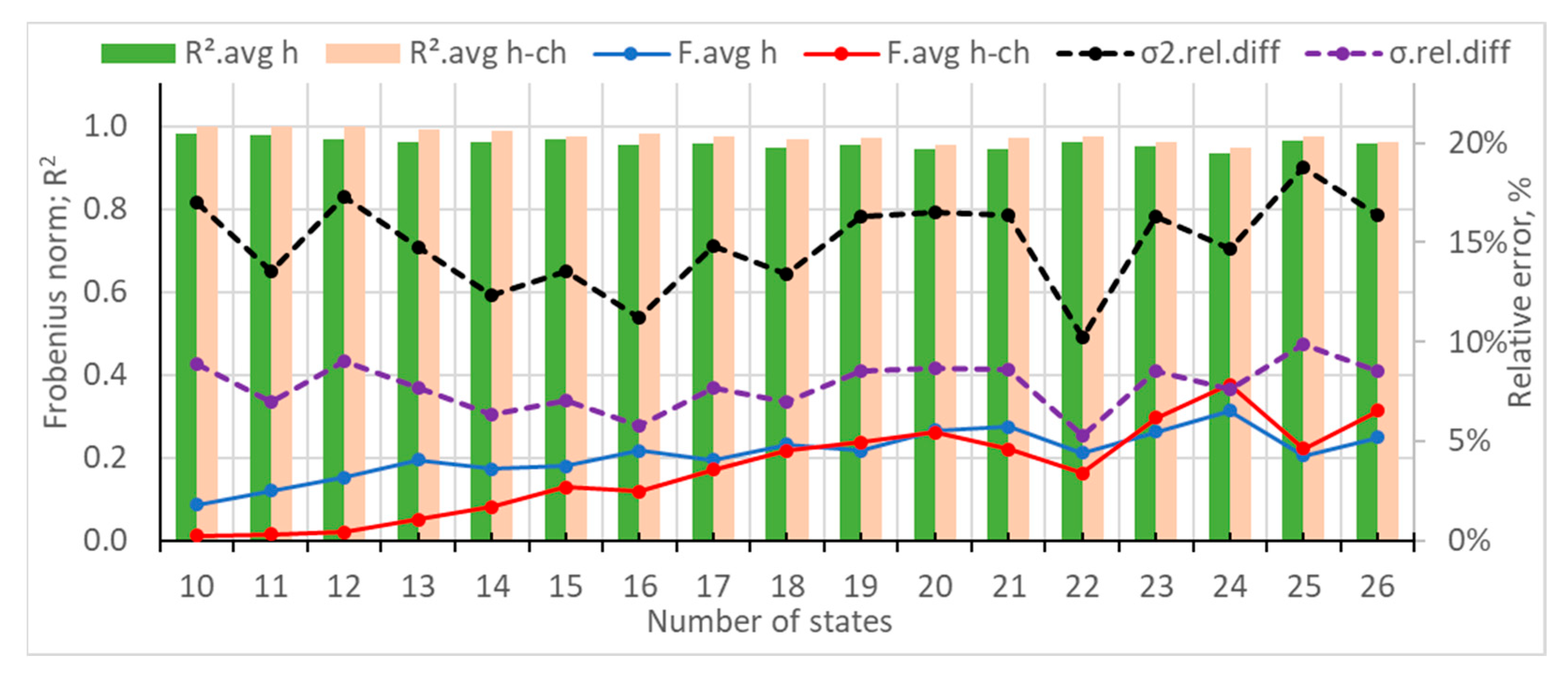
3.2.2. Case Study 2: Generation of Synthetic Power Consumption Data for a Pig Farm

A similar comparison was performed for the pig farm dataset. Once again, the number of states varied between 10 and 26, and for each one, steps 2, 3.1, and 3.2 from the methodology were implemented. The results from the analysis are summarized in Figure 10.

It can be seen that the lowest average hourly Frobenius distances were achieved for 10, 11, and 12 states, though there was also a minimum at 17 states and 23 states. Similarly, the lowest average hour-change Frobenius distances were achieved at 10, 11, and 12 states, and local minimums can be observed at 17 and 24 states. The average hourly and hour-change R² values also had the highest values at 10, 11, and 12 states, yet local maximums can be observed at 17, 23, and 24 states.

Regarding the statistical measures, the relative difference of the variance had a minimum at 21 states, and local minimums at 14 and 23 states. Similarly, the relative difference of the standard deviation had a minimum at 15, 16, and 17 states and local minimums at 19, 22, and 24 states. However, it should be noted that the relative errors in all cases were below 5%.

Once again, there is no ideal number of states for which all measures are optimal, and therefore, the following situations were further investigated (

Table 3. Comparison between the metrics of the three generated datasets of the agricultural consumer with 12, 17, and 23 states.

Metric	Synthetic Data with 12 States	Synthetic Data for 17 States	Synthetic Data for 23 States
Average Frobenius distance of the hourly matrices (F.avg h)	0.18	0.26	0.44
Average Frobenius distance of the hour-change matrices (F.avg h-ch)	0.04	0.35	0.37
Average R2 of the hourly matrices (R2.avg h)	0.97	0.95	0.93
Average R2 of the hour-change matrices (R2.avg h-ch)	0.99	0.93	0.94
Relative error of the variance (σ2.rel.diff)	2.69%	1.58%	0.41%
Relative error of the standard deviation (σ.rel.diff)	0.38%	0.17%	0.74%

):

• the generated data with 12 states, for which all measures except for the variance have near-optimal values;
• the generated data for 17 states, for which all measures except the variance have a local peak value;
• the generated data for 23 states, for which there are local peak values for the Frobenius distances, R², and the variance.

It can be seen that for the investigated agricultural consumer, the probabilistic metrics generally increased with the number of states, though the relative error of the variance decreased. Therefore, to better understand the difference between the selected scenarios, seven days of data were generated for each one of them to perform a visual comparison (Figure 11). It can be visually observed that in all cases, the generated data greatly resembled the original one; nevertheless, with the increase in the number of states, the scattering of the data was lower and better matched the original dataset. This allowed us to make the conclusion that when the evaluation metrics are similar, the scenario with higher number of states should be preferred.

3.2.3. Case Study 3: Generation of Synthetic Power Consumption Data for a Printing House

The third case study concerns the power consumption of a printing house. Using the same methodology, the probabilistic and statistical measures of the generated data with different numbers of states are summarized in Figure 12.

It can be seen that both Frobenius distances had their lowest average values at 10, 11, and 12 states. Thereafter, they had local minimums at 22 and 25 states. It can be noticed that in all cases, they did not surpass 0.4. Analogous observations can be made for the average hourly and hour-change R² coefficients, which did not fall below 0.94 and 0.95, respectively. The variance changed between 10% and 19% and had local minimums at 11, 16, and 22 states. Similarly, the standard deviation changed between 5% and 10% and had local minimums at 11, 16, and 22 states.

Considering the abovementioned, the following situations were selected for closer examination (

Table 4. Comparison between the metrics of the three generated datasets of the industrial consumer with 11, 16, and 22 states.

Metric	Synthetic Data with 11 States	Synthetic Data for 16 States	Synthetic Data for 22 States
Average Frobenius distance of the hourly matrices (F.avg h)	0.12	0.22	0.21
Average Frobenius distance of the hour-change matrices (F.avg h-ch)	0.02	0.12	0.16
Average R2 of the hourly matrices (R2.avg h)	0.98	0.95	0.96
Average R2 of the hour-change matrices (R2.avg h-ch)	1.00	0.98	0.98
Relative error of the variance (σ2.rel.diff)	13.51%	11.18%	10.21%
Relative error of the standard deviation (σ.rel.diff)	7.00%	5.76%	5.24%

):

• the generated data with 11 states, for which all indicators have peaks or close-to-optimal values;
• the generated data with 16 states, for which the statistical measures have local minimums and the probabilistic measures are close to optimal;
• the generated data with 22 states, for which the Frobenius distances and the R² coefficients have local peaks, and the statistical measures have minimums.

It can be seen that the metrics for the three cases were very similar, and once again, the probabilistic ones became slightly worse with the increase in the number of states, while the statistical ones improved. Therefore, seven days of data were generated for each scenario to get a better understanding of their performance (Figure 13). The main problem that can be observed with fewer states was the wider scattering of the data for non-working hours, when it should have been close to zero. The problem was mitigated for the situation with 22 states, which can be explained by the narrower width of the zone. Once again, it can be concluded that when the evaluation metrics are similar, it is better to generate the synthetic data with a higher number of states.

3.3. Discussion and General Recommendations for the Application of the Proposed Methodology

The results obtained from the three case studies allow us to make general recommendations for the application of the proposed methodology. The generation of realistic synthetic data about the power consumption of a consumer depends on the chosen number of states. On the one hand, it is important to make sure the following requirements are met:

• The Frobenius distances, describing the difference between the transition matrices of the original dataset and of the generated data, are as close as possible to 0.
• The R² coefficients, describing how well the generated transition matrices describe the original ones, are as close as possible to 1.
• The statistical measures of the generated data, such as its variance and standard deviation, are as close as possible to the statistical measures of the original dataset.

However, the obtained results also showed that

• The Frobenius distances and R² coefficients were usually closer to their optimal values for a lower number of states.
• The difference between the statistical measures of the generated and original datasets could vary in a wide range, depending on the number of states of the transition matrices.
• The generated datasets with a lower number of states were usually more scattered than the training ones.

In other words, it is not always possible to make sure all of the above requirements are met at the same time. In this case, it is necessary to choose appropriate criteria for optimality. Based on the obtained results, we suggest the following methodology for choosing the optimal number of states:

• Local minimums of the average Frobenius distances and/or local maximums of the average R² coefficients should be looked for at a higher number of states of the transition matrices. It is recommended that the number of states be more than 20 or at least 15.
• Local minimums of the statistical measures of variance and/or standard deviation could be looked for.
• The optimal number of states can be chosen for the situation where the measures from p. 1 and p. 2 have their local peak values or values that are very close to them.

There is another opportunity to mitigate the earlier-mentioned problem, which is expressed in greater scattering of the generated data when fewer states of the transition matrices are used. According to the presented methodology, once the new state of power consumption is chosen, the specific value within the boundary of this state is generated with a uniform distribution. This part of the methodology could be altered to generate random numbers with an appropriate frequency distribution. To do this, an individual frequency distribution should be obtained for each state of each matrix (i.e., for each hour of the day or a total of 24 × N number of distributions), based on the training data. In theory, this could allow generating synthetic data that are very similar to the original one, using fewer states. This approach could be useful when the training data are limited; however, this would also require splitting each state into substates for the frequency distribution, which additionally complicates the algorithm.

4. Conclusions

The development of digital energy systems relies on actual data about the power consumption and generation, which is not always available and is often limited. In such situations, synthetic data are sometimes used that fill in the missing gaps or create long-term simulation data. This study presents a method for generating synthetic load profiles, which is based on the theory of Markov chains. Unlike previous studies, we divided the input time series into hourly and hour-change data on a monthly basis. This way, for each investigated dataset, a total of 48 transition matrices are generated (24 hourly and 24 h-change ones), which are used for generating the synthetic load profile.

The similarity in the statistical and probabilistic parameters between the original and generated data was assessed using several measures: the Frobenius distance, the R² coefficient, relative differences in the variance, and standard deviation. Three case studies with different types of consumers were investigated to demonstrate the application of the methodology. Based on the obtained results, the following recommendations can be made for ensuring high probabilistic and statistical similarity:

• When possible, the number of states of the transition matrices should be 15 or more to reduce the scattering of the synthetic data.
• The number of states can be chosen by looking for local peaks of the Frobenius distance, R² coefficients, relative differences of the variance, and/or standard deviation, which do not differ significantly from their optimal values.

To properly position the proposed model, it is important to compare its performance against models developed by other authors. However, this cannot be directly done because previous studies did not investigate the probabilistic aspects of their results. Therefore, to conduct such a comparison, it is necessary to implement the different models (ML and Markov chain-based ones) and compare their performance against the same datasets using the same probabilistic and statistical measures. Considering the complexity and scale of this task, it is an object for future research. The results achieved in this study can be used by experts involved in designing systems with renewable energy sources and by scientists dealing with long-term studies.

References

1. Endres, M.; Mannarapotta, V.A.; Tran, T.S. Synthetic data generation: A comparative study. In Proceedings of the 26th International Database Engineered Applications Symposium, Budapest, Hungary, 22–24 August 2022; pp. 94–102. [Google Scholar]
2. Sandhaas, A.; Kim, H.; Hartmann, N. Methodology for Generating Synthetic Load Profiles for Different Industry Types. Energies 2022, 15, 3683. [Google Scholar] [CrossRef]
3. Jordon, J.; Szpruch, L.; Houssiau, F.; Bottarelli, M.; Cherubin, G.; Maple, C.; Cohen, S.; Weller, A. Synthetic Data—What, Why and How? Royal Society: London, UK, 2022; Available online: https://royalsociety.org/-/media/policy/projects/privacy-enhancing-technologies/Synthetic_Data_Survey-24.pdf (accessed on 15 March 2025).
4. Hong, T.; Pinson, P.; Wang, Y.; Weron, R.; Yang, D.; Zareipour, H. Energy forecasting: A review and outlook. IEEE Open Access J. Power Energy 2020, 7, 376–388. [Google Scholar] [CrossRef]
5. Proedrou, E. A comprehensive review of residential electricity load profile models. IEEE Access 2021, 9, 12114–12133. [Google Scholar] [CrossRef]
6. Viana, D.; Teixeira, R.; Baptista, J.; Pinto, T. Synthetic Data Generation Models for Time Series: A Literature Review. In Proceedings of the 2024 International Conference on Electrical, Computer and Energy Technologies (ICECET), Sydney, Australia, 25–27 July 2024; pp. 1–6. [Google Scholar] [CrossRef]
7. Bauer, A.; Trapp, S.; Stenger, M.; Leppich, R.; Kounev, S.; Leznik, M.; Foster, I. Comprehensive exploration of synthetic data generation: A survey. arXiv 2024, arXiv:2401.02524. [Google Scholar] [CrossRef]
8. Lu, Y.; Shen, M.; Wang, H.; Wang, X.; van Rechem, C.; Fu, T.; Wei, W. Machine learning for synthetic data generation: A review. arXiv 2023, arXiv:2302.04062. [Google Scholar] [CrossRef]
9. Jacobsen, B.N. Machine learning and the politics of synthetic data. Big Data Soc. 2023, 10, 20539517221145372. [Google Scholar] [CrossRef]
10. Gandoman, F.H.; Aleem, S.H.A.; Omar, N.; Ahmadi, A.; Alenezi, F.Q. Short-term solar power forecasting considering cloud coverage and ambient temperature variation effects. Renew. Energy 2018, 123, 793–805. [Google Scholar] [CrossRef]
11. Triastcyn, A.; Faltings, B. Generating Higher-Fidelity Synthetic Datasets with Privacy Guarantees. Algorithms 2022, 15, 232. [Google Scholar] [CrossRef]
12. Zaini, F.A.; Sulaima, M.F.; Razak, I.A.W.A.; Othman, M.L.; Mokhlis, H. Improved Bacterial Foraging Optimization Algorithm with Machine Learning-Driven Short-Term Electricity Load Forecasting: A Case Study in Peninsular Malaysia. Algorithms 2024, 17, 510. [Google Scholar] [CrossRef]
13. Lázaro, C.; Angulo, C. Iterative Application of UMAP-Based Algorithms for Fully Synthetic Healthcare Tabular Data Generation. Algorithms 2024, 17, 591. [Google Scholar] [CrossRef]
14. Yue, Y.; Li, Y.; Yi, K.; Wu, Z. Synthetic data approach for classification and regression. In Proceedings of the 2018 IEEE 29th International Conference on Application-specific Systems, Architectures and Processors (ASAP), Milan, Italy, 10–12 July 2018; IEEE: New York, NY, USA, 2018; pp. 1–8. [Google Scholar] [CrossRef]
15. Goyal, M.; Mahmoud, Q.H. A Systematic Review of Synthetic Data Generation Techniques Using Generative AI. Electronics 2024, 13, 3509. [Google Scholar] [CrossRef]
16. Pan, Z.; Wang, J.; Liao, W.; Chen, H.; Yuan, D.; Zhu, W.; Fang, X.; Zhu, Z. Data-Driven EV Load Profiles Generation Using a Variational Auto-Encoder. Energies 2019, 12, 849. [Google Scholar] [CrossRef]
17. Wang, C.; Tindemans, S.H.; Palensky, P. Generating contextual load profiles using a conditional variational autoencoder. In Proceedings of the 2022 IEEE PES Innovative Smart Grid Technologies Conference Europe (ISGT-Europe), Novi Sad, Serbia, 10–12 October 2022; IEEE: New York, NY, USA, 2022; pp. 1–6. [Google Scholar] [CrossRef]
18. Hu, Y.; Kim, H.; Ye, K.; Lu, N. Applying fine-tuned LLMs for reducing data needs in load profile analysis. Appl. Energy 2025, 377, 124666. [Google Scholar] [CrossRef]
19. Turowski, M.; Heidrich, B.; Weingärtner, L.; Springer, L.; Phipps, K.; Schäfer, B.; Hagenmeyer, V. Generating synthetic energy time series: A review. Renew. Sustain. Energy Rev. 2024, 206, 114842. [Google Scholar] [CrossRef]
20. Yilmaz, B.; Korn, R. Synthetic demand data generation for individual electricity consumers: Generative Adversarial Networks (GANs). Energy AI 2022, 9, 100161. [Google Scholar] [CrossRef]
21. Asre, S.; Anwar, A. Synthetic Energy Data Generation Using Time Variant Generative Adversarial Network. Electronics 2022, 11, 355. [Google Scholar] [CrossRef]
22. Fekri, M.N.; Ghosh, A.M.; Grolinger, K. Generating Energy Data for Machine Learning with Recurrent Generative Adversarial Networks. Energies 2020, 13, 130. [Google Scholar] [CrossRef]
23. Figueira, A.; Vaz, B. Survey on Synthetic Data Generation, Evaluation Methods and GANs. Mathematics 2022, 10, 2733. [Google Scholar] [CrossRef]
24. Zhang, C.; Kuppannagari, S.R.; Kannan, R.; Prasanna, V.K. Generative adversarial network for synthetic time series data generation in smart grids. In Proceedings of the 2018 IEEE International Conference on Communications, Control, and Computing Technologies for Smart Grids (SmartGridComm), Aalborg, Denmark, 29–31 October 2018; IEEE: New York, NY, USA, 2018; pp. 1–6. [Google Scholar] [CrossRef]
25. Stoyanov, L.; Draganovsk, I. Application of ANN for forecasting of PV plant output power–Case study Oryahovo. In Proceedings of the 2021 17th Conference on Electrical Machines, Drives and Power Systems (ELMA), Sofia, Bulgaria, 1–4 July 2021; pp. 1–5. [Google Scholar] [CrossRef]
26. Stoyanov, L.; Draganovska, I. Comparison of Hybrid Models for PV Power Output Forecasting—Application to Oryahovo, Bulgaria. In Proceedings of the 2023 18th Conference on Electrical Machines, Drives and Power Systems (ELMA), Varna, Bulgaria, 29 June–1 July 2023; pp. 1–4. [Google Scholar] [CrossRef]
27. McLoughlin, F.; Duffy, A.; Conlon, M. The generation of domestic electricity load profiles through Markov chain modelling. In Proceedings of the 3rd International Scientific Conference on Energy and Climate Change Conference, Athens, Greece, 7–8 October 2010; pp. 18–27. [Google Scholar]
28. Radet, H.; Sareni, B.; Roboam, X. Synthesis of Solar Production and Energy Demand Profiles Using Markov Chains for Microgrid Design. Energies 2023, 16, 7871. [Google Scholar] [CrossRef]
29. Tushar, W.; Huang, S.; Yuen, C.; Zhang, J.A.; Smith, D.B. Synthetic generation of solar states for smart grid: A multiple segment Markov chain approach. In Proceedings of the IEEE PES Innovative Smart Grid Technologies, Europe, Istanbul, Turkey, 12–15 October 2014; IEEE: New York, NY, USA, 2014; pp. 1–6. [Google Scholar] [CrossRef]
30. Bai, J. Markov model in home energy management system. J. Phys. Conf. Ser. 2021, 1871, 012043. [Google Scholar] [CrossRef]
31. Meidani, H.; Ghanem, R. Multiscale Markov models with random transitions for energy demand management. Energy Build. 2013, 61, 267–274. [Google Scholar] [CrossRef]
32. Evstatiev, B.; Beleov, I.; Gabrovska, K. Probabilities for prolonged periods of low and high energy output from photovoltaic generators in Ruse. Ecologica 2015, 22, 192–195. [Google Scholar]
33. Evstatiev, B.; Beloev, I. Evaluation of the probabilities for prolonged periods of high and low energy output of wind turbines. Ecologica 2015, 22, 5–11. [Google Scholar]
34. Zuo, W.M.; Wang, K.Q.; Zhang, D. Assembled matrix distance metric for 2DPCA-based face and palmprint recognition. In Proceedings of the 2005 International Conference on Machine Learning and Cybernetics, Guangzhou, China, 18–21 August 2005; IEEE: New York, NY, USA, 2005; Volume 8, pp. 4870–4875. [Google Scholar] [CrossRef]
35. Di Bucchianico, A. Coefficient of determination (R2). Encyclopedia of statistics in quality and reliability. In Encyclopedia of Statistics in Quality and Reliability; Wiley: Hoboken, NJ, USA, 2008. [Google Scholar] [CrossRef]
36. Indrayan, A.; Holt, M.P. Concise encyclopedia of biostatistics for medical professionals. In Concise Encyclopedia of Biostatistics for Medical Professionals; Chapman and Hall: Boca Raton, FL, USA; CRC: Long Beach, CA, USA, 2016. [Google Scholar] [CrossRef]
Figure 1. Example of load profiles with the same statistical characteristics but different probabilistic characteristics: (a) the load profile crosses the 2 kW level 6 times; (b) the load profiles crosses the 2 kW level 2 times.
Algorithms 18 00287 g001
Figure 2. A summary of the methodology for synthetic data generation.
Algorithms 18 00287 g002
Figure 3. Classification of the load profile’s discrete samples into N states.
Algorithms 18 00287 g003
Figure 4. Generation of the transition matrices for each hour of the day and for each hour-change.
Algorithms 18 00287 g004
Figure 5. A screenshot from the developed software tool for the generation and comparison of synthetic load profiles.
Algorithms 18 00287 g005
Figure 6. Sample datasets with the power consumption of (a) a domestic house; (b) a pig farm; (c) a printing house.
Algorithms 18 00287 g006
Figure 7. Hourly Frobenius distances and R2 coefficients of the generated data with 12 states.
Algorithms 18 00287 g007
Figure 8. Dependency of the average Frobenius distances, average R2s, relative difference of the variance, and standard deviation for the investigated number of states of the synthetic data for a domestic house.
Algorithms 18 00287 g008
Figure 9. Seven days of sample data from the original time series for a house (a) and from the generated synthetic data with 12 states (b), 18 states (c), and 24 states (d).
Algorithms 18 00287 g009
Figure 10. Dependency of the average Frobenius distances, average R2s, relative differences of the variance, and standard deviation for the different number of states of the synthetic data of a pig farm.
Algorithms 18 00287 g010
Figure 11. Seven days of sample data from the original time series for a pig house (a), and from the generated synthetic data for 12 states (b), 17 states (c), and 23 states (d).
Algorithms 18 00287 g011
Figure 12. Dependency of the average Frobenius distances, average R2s, the relative differences of variance, and standard deviation for the different number of states of the synthetic data for a printing house.
Algorithms 18 00287 g012
Figure 13. Seven days of sample data from the original time series for a printing house (a), and from the generated synthetic data for 11 states (b), 16 states (c), and 22 states (d).
Algorithms 18 00287 g013