Mathematics-Driven Analysis of Offshore Green Hydrogen Stations

Abstract

Renewable energy technologies have become an increasingly important component of the global energy supply. In recent years, photovoltaic and wind energy have been the fastest-growing renewable sources. Although oceans present harsh environments, their estimated energy generation potential is among the highest. Ocean-based solutions are gaining significant momentum, driven by the advancement of offshore wind, floating solar, tidal, and wave energy, among others. The integration of various marine energy sources with green hydrogen production can facilitate the exploitation and transportation of renewable energy. This paper presents a mathematics-driven analysis for the simulation of a technical model designed as a generic framework applicable to any location worldwide and developed to analyze the integration of solar energy generation and green hydrogen production. It evaluates the impact of key factors such as solar irradiance, atmospheric conditions, water surface flatness, as well as the parameters of photovoltaic panels, electrolyzers, and adiabatic compressors, on both energy generation and hydrogen production capacity. The proposed mathematics-based framework serves as an innovative tool for conducting multivariable parametric analyses, selecting optimal design configurations based on specific solar energy and/or hydrogen production requirements, and performing a range of additional assessments including, but not limited to, risk evaluations, cause–effect analyses, and/or degradation studies. Enhancing the efficiency of solar energy generation and hydrogen production processes can reduce the required photovoltaic surface area, thereby simplifying structural and anchoring requirements and lowering associated costs. Simpler, more reliable, and cost-effective designs will foster the expansion of floating solar energy and green hydrogen production in marine environments.

1. Introduction

Renewable energies are those obtained from virtually inexhaustible natural sources, either due to the immense amount of energy they contain or because they can regenerate naturally [1,2]. Among the main sources of renewable energy are solar energy, wind energy, hydroelectric energy, geothermal energy, biomass, tidal, and wave energy [3,4].

Interest and investment in renewable energies have experienced exponential growth in recent decades [5], driven by increasing concerns about climate change and the need to reduce greenhouse gas emissions [6,7]. According to the International Renewable Energy Agency (IRENA) [8], global renewable energy generation capacity reached 3.86 TW by the end of 2023, representing a cumulative growth of 127.55% since 2014, when it stood at 1.7 TW. Over this period, the average annual growth rate was 9.58%. Notably, between 2022 and 2023 alone, the annual growth rate reached 13.95%. These energy sources offer a clean and sustainable alternative to traditional fossil fuels such as oil, coal, and natural gas, which, in addition to being finite, contribute negatively to global warming when burned [9,10].

Moreover, renewable energies provide countries that adopt them with greater energy security by strategically and systematically reducing their dependence on imported and volatile resources [11]. The installation of offshore renewable energy systems presents enormous potential for a sustainable energy future [12,13]. Offshore renewable technologies represent a promising frontier in the development of clean energy, harnessing the vast energy resources available in the world’s oceans and seas [14,15]. These technologies not only offer significant potential for clean energy generation but also provide unique advantages compared to their onshore counterparts [16,17]. The potential of marine energy is estimated to range between 45.000 TWh and 130.000 TWh of electricity per year. However, as of now, only 508 MW of the total global capacity is being supplied by marine energy generators [18].

As of today, photovoltaic energy (1.42 TW) and wind energy (1.01 TW) are the two renewable sources contributing most significantly to global renewable energy capacity. Over the past decade, their cumulative growth has been approximately 706% and 191%, respectively. At the end of 2023, onshore wind energy capacity reached 944.2 GW, while offshore wind capacity amounted to 73.18 GW. Nonetheless, despite the substantial difference in their current capacities, onshore wind energy has exhibited a cumulative growth rate of 176.93%, while offshore wind has experienced a remarkable increase of 760.80% [8]. This significant trend underscores the growing influence that ocean-based solutions are expected to have on the near-term future of renewable energy.

Floating solar energy is emerging as a strategic and innovative solution to address the global energy crisis and the increasing scarcity of land available for renewable energy deployment. Its development is particularly crucial for countries facing territorial constraints, high energy demand, or densely populated coastal areas [19,20,21]. Although most floating energy systems currently operate in freshwater environments such as lakes and reservoirs, the technical and geographical potential of the marine environment is driving the development of offshore projects, including Swimsol (Maldives), Ocean Sun (Norway/China), and SolarDuck (Europe). These projects also serve as platforms for exploring various structural configurations, such as rigid and flexible designs [19].

Among the most notable advantages of floating solar energy are the preservation of arable land, the reduction in water evaporation, and the improvement of water quality by limiting algal growth. Additionally, co-location with other types of infrastructure—such as onshore or offshore wind farms—can optimize space usage and enable the sharing of electrical equipment, thereby enhancing the overall stability and efficiency of the energy system [19]. Floating solar energy systems are estimated to exhibit higher efficiency than their land-based counterparts, reaching gains of up to 11–13% or more. This improvement is primarily attributed to the cooling effect provided by the water surface and the natural cleaning of the panels [20,21]. It is also estimated that the natural cooling of solar panels by approximately 2.7–3.5 °C results in a daily efficiency increase of around 2.3–2.6% [19].

In terms of disadvantages, the main challenges are associated with the marine environment: saltwater-induced corrosion, difficulties in remote maintenance, high anchoring costs, and the need to ensure structural stability under extreme wind and wave conditions [19]. In terms of cost, offshore systems still present a higher Levelized Cost of Electricity (LCOE) compared to land-based systems—approximately 2.5% higher. However, this cost is expected to decrease as production scales up and technologies such as thin-film panels and flexible structures are increasingly adopted [19].

In parallel, hydrogen has emerged as a promising energy carrier in the transition toward a more sustainable and carbon-free future [22]. Unlike primary energy sources, hydrogen functions as an energy carrier, enabling the storage and transportation of energy produced by other sources. Its versatility lies in the fact that it can be obtained from various primary sources, and, when produced using renewable energy, it becomes green hydrogen—a clean and sustainable alternative [22,23,24].

Green hydrogen is primarily produced through the electrolysis process, driven by different electrolyzer technologies. In alkaline electrolyzers (ALK), an aqueous potassium hydroxide solution is used as the electrolyte, while, in proton exchange membrane (PEM) electrolyzers, the electrolyte is a thin, ion-conductive solid membrane that replaces the aqueous solution. Both technologies require electricity generated from renewable sources, such as solar or wind energy [25], to split the water molecule (H₂O) into oxygen (O₂) and hydrogen (H₂) [26]. This production method ensures that no pollutant gases are emitted either during the production process (energy generation and storage) or during combustion (extraction and use of stored energy). Moreover, green hydrogen offers significant advantages, including its storage capacity—high energy density per kilogram—and its versatility to be converted into electricity or synthetic fuels, making it an attractive option for various industrial and mobility sectors [27].

The importance of green hydrogen in combating climate change lies in its potential to replace fossil fuels in hard to decarbonize sectors [24]. However, the development of green hydrogen faces challenges, primarily related to production costs and the need for expanded infrastructure. As progress is made in decarbonization and the cost of renewable energy generation decreases, these obstacles are expected to be overcome, allowing green hydrogen to play a crucial role in the global energy transition [26,28]. In this context, the present article aims to promote the expansion and use of floating solar energy through the development of a mathematics-based technical model that enables the analysis of its integration with green hydrogen production stations [29], the assessment of energy efficiency gains resulting from increased solar irradiance in marine locations, as well as the impact of component efficiencies and key operating parameters in the green hydrogen production station (photovoltaic panels, electrolyzer, and compressor), on the total required surface area of photovoltaic panels. This reduction will not only simplify the support and anchoring structures of floating solar power stations but also reduce overall costs and improve structural stability under extreme wind and wave conditions. For these reasons, a mathematics-based technical model of a green hydrogen production station powered by solar energy is presented to be used as a generic framework applicable to any location worldwide. This station can be equipped with two types of electrolyzers (Figure 1): alkaline (ALK) and proton exchange membrane (PEM).

By integrating green hydrogen production with the electricity generation capacity of solar energy, production becomes decentralized and more flexible, allowing for installation in both onshore—freshwater—and offshore environments. Some of the additional benefits that can be achieved through the use of this type of offshore stations are as follows: (i) it enables hydrogen production near potential consumption points—such as oil platforms, ships, or coastal facilities—significantly reducing the need for long-distance hydrogen transportation and storage, along with the associated costs and risks, and supporting the integration of green hydrogen into existing maritime operations.

Additionally, the ability to store and transport the produced green hydrogen reduces the need for installing underwater cables for energy transmission: (ii) It ensures and facilitates access to the primary resource from which green hydrogen is extracted: water (H₂O). The extraction of seawater ensures a reliable and virtually inexhaustible supply, regardless of the hydrogen production levels required at its output. (iii) As demonstrated throughout this study, it ensures an increase in green hydrogen production capacity, driven by the reflection of solar radiation on the sea surface and the lower atmospheric attenuation of solar radiation due to reduced pollution levels—compared to other onshore locations [21].

This increase in production capacity can be leveraged in two distinct ways: (i) by increasing the station’s green hydrogen output while maintaining the same photovoltaic surface area or (ii) by maintaining the same station’s hydrogen output and reducing the surface area required for the solar panels. Given the harsh conditions of the marine environment, reducing the size of the solar panels surface simplifies the structural and anchoring requirements, thereby lowering associated costs. Simpler, more reliable, and cost-effective designs will foster the expansion of floating solar energy and green hydrogen production in marine environments.

2. Materials and Methods

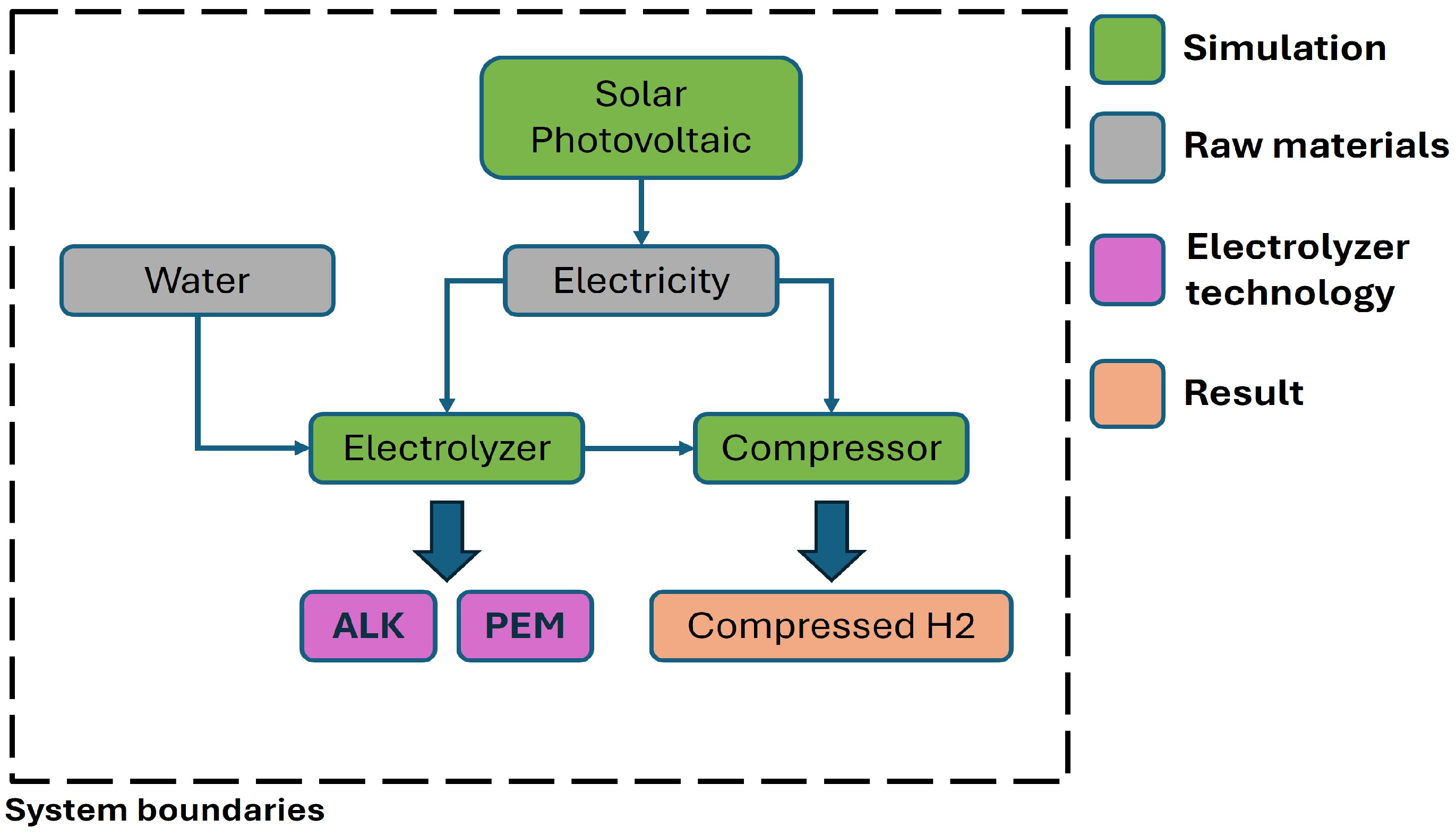
2.1. Mathematics-Driven Analysis and Simulation Method

The following sections present the mathematics-based technical model proposed in this paper. A set of input parameters and mathematical expressions were used to describe the physical relationships among the different components of the system. To perform the simulation and subsequent analysis of the results, these expressions were implemented using Python 3.12 as programming language, which is widely adopted in both scientific and industrial communities. Python, as an open-source solution from the Python Software Foundation, provides a broad range of scientific and visualization libraries, making it ideal for performing complex calculations and processing the data required at each phase of the simulation. In addition, this Python-based approach not only enhances the model’s accuracy and flexibility but also facilitates its adaptation to different scenarios and conditions, which is an essential feature for optimizing the design and operation of current and future offshore renewable energy systems.

Due to Python’s handling of trigonometric functions, all angles used as input parameters for these mathematical expressions are expressed in radians (rad). However, for ease of interpretation and visualization, all other angles are presented in degrees (°). All external and internal technical model variables introduced throughout this paper are listed and summarized in the Abbreviations Section.

The development of the mathematics-based technical model and its subsequent validation through the execution of a set of numerical simulations requires a logical and structured approach, consisting of distinct phases that simplify the original problem while preserving the sequential and/or parallel relationships among their components. Figure 2 presents the high-level flow diagram used for the development and simulation of the proposed technical model for a green hydrogen production station powered by solar energy.

The main sets of parameters used for model configuration are shown in green (also see Section 2.2). In red, the main outputs of the proposed technical model are represented. As part of the methodology presented in this paper, five phases were defined and are represented in yellow, purple, blue, and orange. As part of each phase, the corresponding block diagram provides a high-level definition and illustrates the physical relationships among the various variables involved.

As shown, in PHASE I, the simulation time frame was defined by setting the total duration and time intervals for the calculations. In PHASE II, the solar-based electricity generation process is modeled. This involves first determining the position of the sun relative to the photovoltaic panels and subsequently calculating the solar radiation received on their surface. To model the sun’s position relative to the photovoltaic panels, it is necessary to determine the following variables: Earth’s declination (${\alpha }_{declination}$), corrected solar angle (${\alpha }_{corrected\_solar}$), solar elevation angle (${\alpha }_{solar\_elevation}$), solar azimuth angle (${\alpha }_{solar\_azimuth}$), photovoltaic panel inclination angle (${\beta }_{inclination}$), and photovoltaic panel inclination angle (${\beta }_{azimuth}$) (Figure 3).

In PHASEs III and IV, the operation of the electrolyzer and compressor were modeled based on their specific operational parameters and efficiencies. Finally, in PHASE V, all component models of the green hydrogen station powered by solar energy were integrated. This phase involves synchronizing the various subsystems to ensure that the energy generated by the photovoltaic panels was appropriately balanced to power both the electrolyzer and the compressor.

2.2. Generalization and Particularization: Mathematics-Based Technical Model Configuration

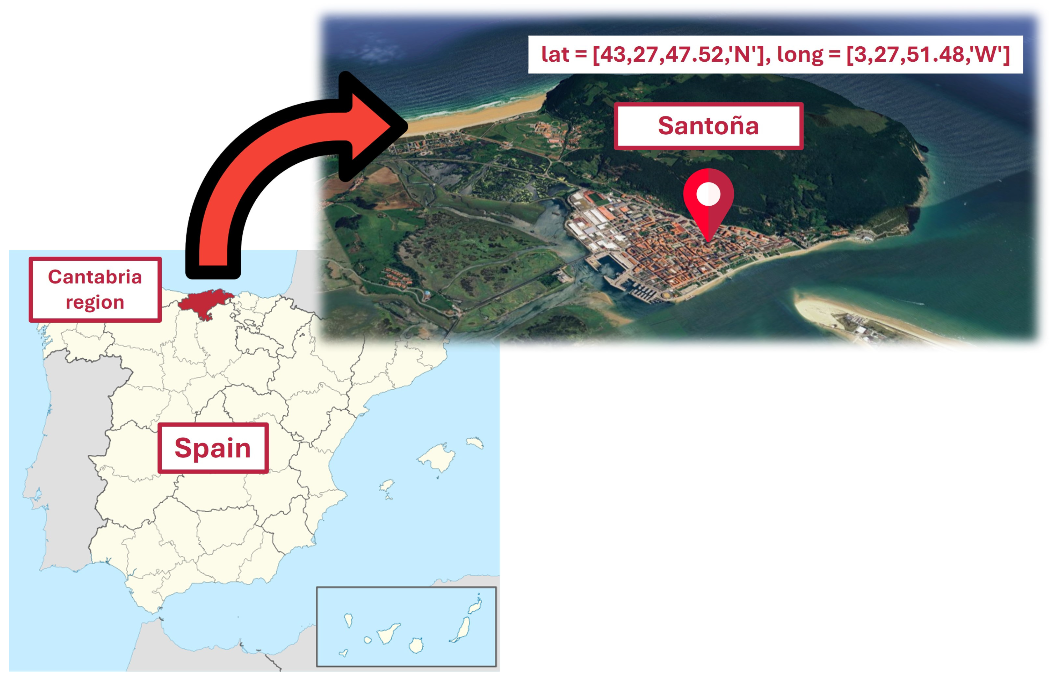
The mathematics-based technical model developed, coded, and simulated throughout this article was designed as a generic framework applicable to any location worldwide and can be tailored to different case studies. For example, it can be used to conduct specific analyses and simulations of solar energy stations integrated with green hydrogen production plants—based on well-defined, pre-established parameters—and/or to evaluate the suitability of those parameters. This can be achieved through multivariable parametric analyses, risk assessments, cause–effect studies, degradation modeling, and other techniques aimed at optimizing parameter selection and overall system performance.

As previously introduced (Figure 2), the proposed technical model can be configured using the following set of input parameters (

Table 1. Configuration parameters of the mathematics-based technical model.

Parameter	Definition
Localization:	Localization of solar panels and green hydrogen station.
Time definition:	Total number of days in a year. Specific day of the year. Day under study. Local time, referenced to 12 p.m.
Atmosphere and marine conditions:	Atmospheric state/quality. Coefficient of losses associated with ocean surface irregularities. Ambient temperature.
Photovoltaic panels:	Photovoltaic panel inclination and azimuth. Energy conversion efficiency.
Electrolyzer:	ALK type. PEM type. Hydrogen calorific power constant. ALK electrolyzer efficiency. PEM electrolyzer efficiency.
Compressor:	Input pressure. Output pressure. Compression efficiency.

).

Based on these configuration parameters, the model enables the determination of the station’s green hydrogen production capacity, expressed in ${\displaystyle \frac{{\mathrm{m}\mathrm{o}\mathrm{l}}_{{\mathrm{H}}_2}}{\mathrm{s}\times {\mathrm{m}}^2}}$ and ${\displaystyle \frac{{\mathrm{k}\mathrm{g}}_{{\mathrm{H}}_2}}{\mathrm{s}\times {\mathrm{m}}^2}}$. Specifically, (i) if a given photovoltaic panel surface area (m²) is set, the model can calculate the amount of hydrogen produced in either ${\displaystyle \frac{\mathrm{m}\mathrm{o}\mathrm{l}}{\mathrm{s}}}$ or ${\displaystyle \frac{\mathrm{k}\mathrm{g}}{\mathrm{s}}}$ or (ii) if a specific hydrogen production rate is set, in ${\displaystyle \frac{\mathrm{m}\mathrm{o}\mathrm{l}}{\mathrm{s}}}$ or ${\displaystyle \frac{\mathrm{k}\mathrm{g}}{\mathrm{s}}}$, the model can determine the required photovoltaic panel surface area (m²) needed to produce that amount of hydrogen. Likewise, the model enables the determination of the water consumption, expressed in ${\displaystyle \frac{{\mathrm{l}}_{{\mathrm{H}}_2\mathrm{O}}}{\mathrm{s}\times {\mathrm{m}}^2}}$, based on the desired green hydrogen production rate.

2.3. Localization

The location where the photovoltaic panels were intended to be installed (or were already installed) was configured using DMS (degrees, minutes, seconds) coordinate format, where degrees (deg), minutes (min), and seconds (s). These coordinates are then automatically converted into decimal (dec) format:

$$dec=deg+{\displaystyle \frac{min}{60}}+{\displaystyle \frac{s}{3600}}$$

(1)

For locations situated north of the Equator, latitude (lat), and east of the Greenwich meridian, longitude (long), the decimal value (dec) is positive (>0); otherwise, it is negative (<0).

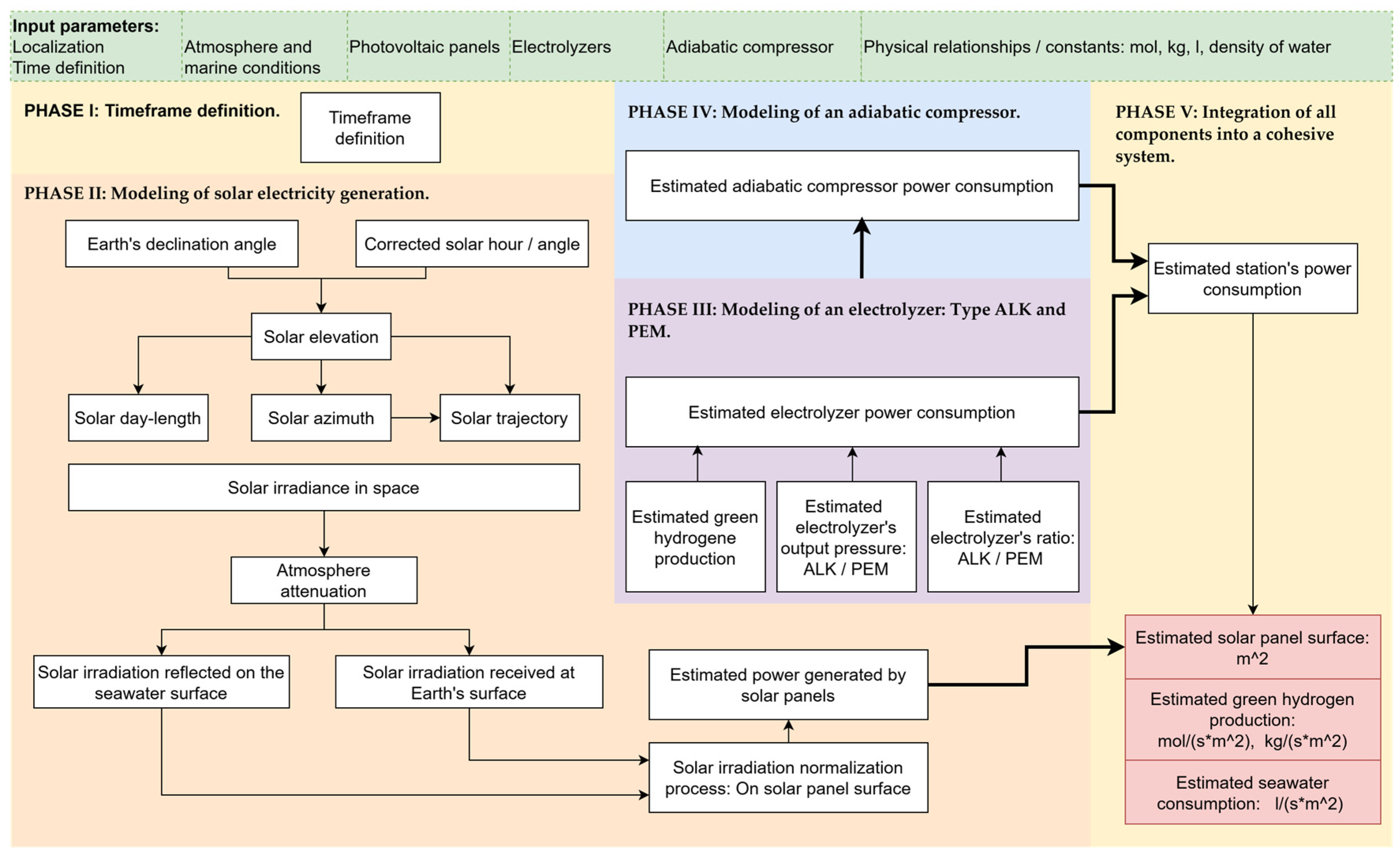
2.4. PHASE I: Timeframe Definition

The simulation and graphical representation of the mathematics-based technical model were performed within a framework that simulates the passage of time. This temporal framework was modeled using a set of numerical values, expressed as an array, which stores the logical relationship between natural time variables: hours, days, months, and years.

2.5. PHASE II: Modeling of Solar Electricity Generation

The sizing of the photovoltaic station required to power the electrolyzer and compressor used in the green hydrogen production process was carried out by the following: (i) calculating the relative position of the sun with respect to the selected location of the station, (ii) determining the solar radiation received perpendicularly on the surface of the photovoltaic panels, and (iii) assessing the panels’ ability to convert solar radiation into electrical energy based on the selected technology per square meter of photovoltaic surface.

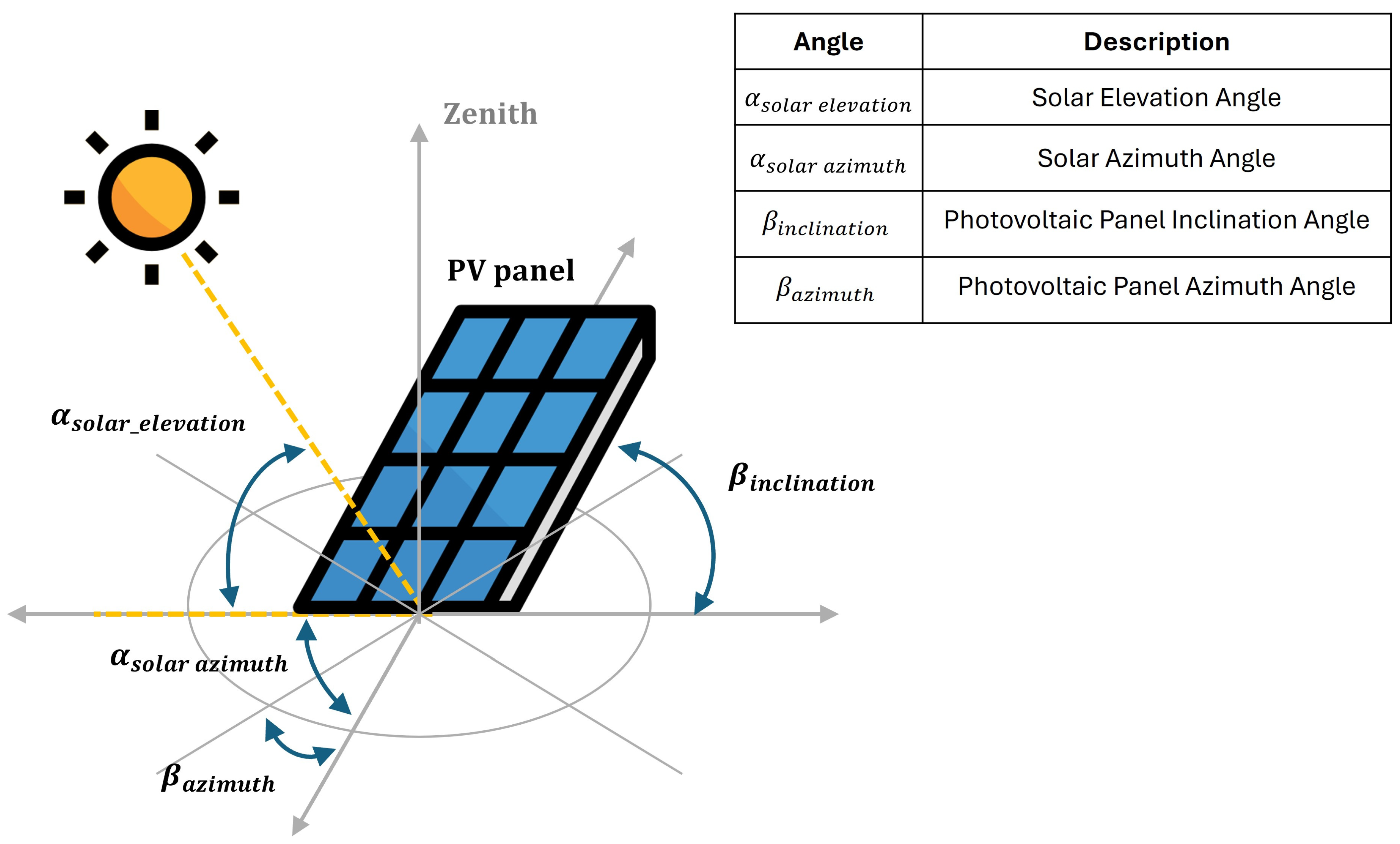
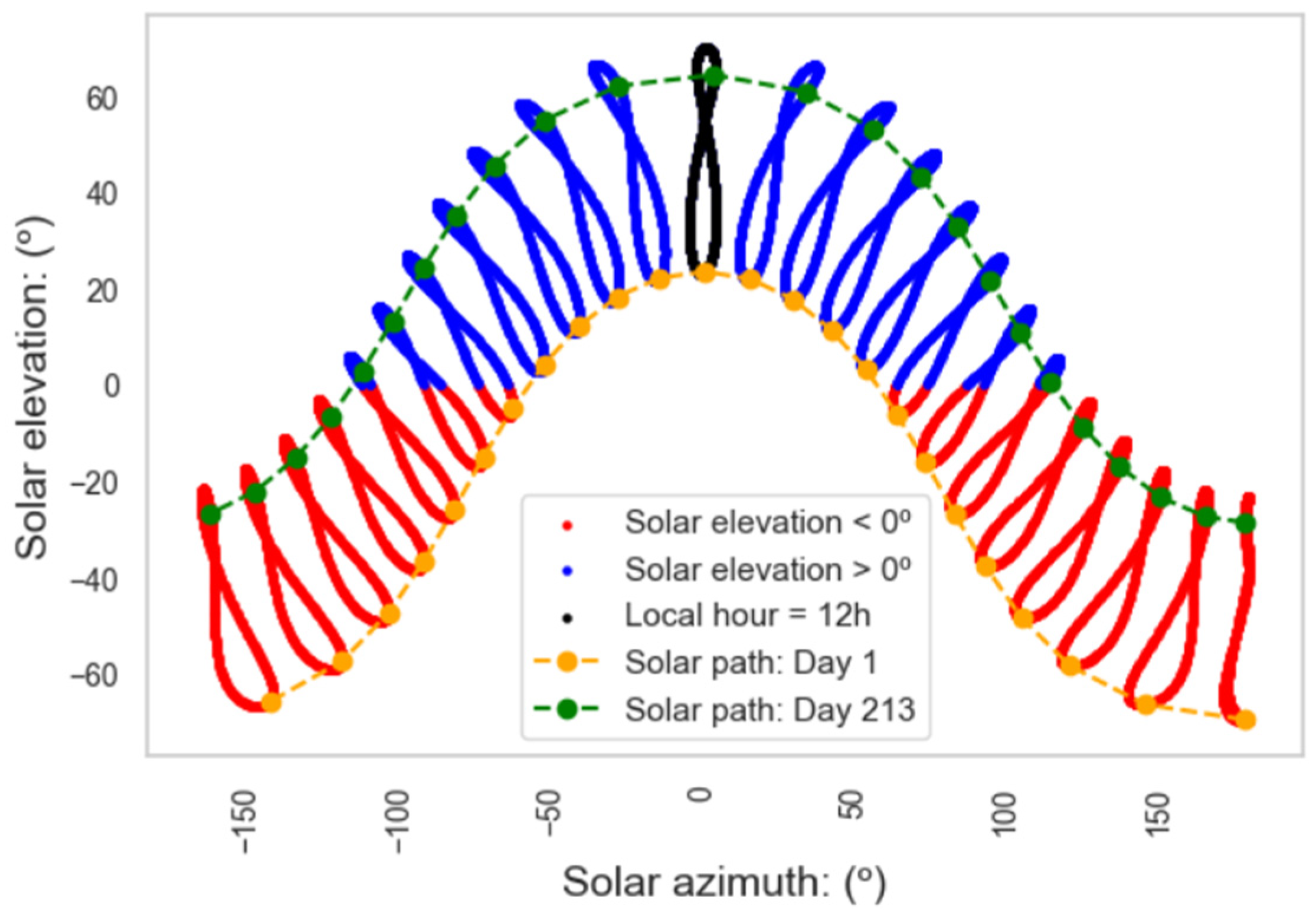
2.5.1. Modeling the Sun’s Position Relative to the Location of the Photovoltaic Panels Powering the Green Hydrogen Station

The first step is to model the set of trigonometric relationships used as the basis for calculating the absolute position of the sun relative to the final selected location of the station [30,31]. These relationships allow for the calculation of the Earth’s declination angle (${\alpha }_{declination}$), solar hour angle (${\alpha }_{solar}$), solar elevation angle (${\alpha }_{solar\_elevation}$), solar azimuth angle (${\alpha }_{solar\_azimuth}$), and the day length ($d_{lenght}$).

${\alpha }_{declination}$ is the tilt angle of the Earth’s rotational axis and is modeled using Cooper’s equation [31]:

$${\alpha }_{declination}=23.45°\times \mathit{sin}\left({\displaystyle \frac{2\ast \pi }{N_{days}}}\times \left( N+C_{equinox} \right)\right)$$

(2)

where $N_{days}$ is the total number of days in the year, N is the day number within the interval [1, $N_{days}$] for which ${\alpha }_{declination}$, is to be calculated, and C_equinox is the synchronization constant of ${\alpha }_{declination}$ with the spring or autumn equinox (Equation (3)). In both cases, since it is a sinusoidal function, the result of the expression (Equation (2)) is synchronized with its zero crossings. ${\alpha }_{declination}$ is a variable with a period of one year and values oscillating between ±23.45° [32].

$$C_{\mathrm{e}\mathrm{q}\mathrm{u}\mathrm{i}\mathrm{n}\mathrm{o}\mathrm{x}}=\begin{array}{c}-81, spring equinox\\ 284, autumm equinox\end{array}$$

(3)

${\alpha }_{solar}$ is calculated relative to the selected location of the station. To perform this, the local time ($h_{local}$) was synchronized with the time of maximum solar elevation (12 p.m.), and the resulting value was multiplied by the number of degrees that the Earth rotates on its axis per hour. Considering that the Earth completes a full 360° rotation every 24 h, ${\alpha }_{solar}$ is modeled as follows:

$${\alpha }_{solar}={\displaystyle \frac{360°}{24}}\times (h_{local}-12)$$

(4)

where $h_{local}$ represents the set of values within the interval [0, 24). By itself, expression (Equation (4)) does not account for the fact that the apparent motion of the sun is not uniform and that the length of the solar day is not constant throughout the year [33]. The modeling of this variation was performed using the general equation of solar time, with results expressed in minutes (min) [31]:

$$\begin{gathered} \nabla t=229.18\times (0.000075+0.001868\times cos(x)-0.032077\times sin(x)-0.014615\times cos(2x) \\ -0.040849\times sin\left(2x\right)) \end{gathered}$$

(5)

where x is an expression calculated as follows:

$$x={\displaystyle \frac{2\pi }{N_{days}}}\times \left( \mathrm{N}-1+{\displaystyle \frac{\left(h_{local}-12\right)}{24}}\right)$$

(6)

By combining equations (Equations (4)–(6)), the corrected solar angle equation (${\alpha }_{solar\_corrected}$) was obtained:

$${\alpha }_{solar\_corrected}={\displaystyle \frac{360°}{24}}\times \left(\right(h_{local}-12)+ {\displaystyle \frac{\nabla t}{60}})$$

(7)

where the value of $\nabla t$ is divided by 60 to convert it to hours (Equation (7)).

The solar elevation angle (${\alpha }_{solar\_elevation}$) is the angle formed by the solar rays with the horizon line as seen from the location of the green hydrogen station. This angle is modeled using a trigonometric relationship that depends on lat (Equation (1)), ${\alpha }_{declination}$ (Equations (2) and (3)), and ${\alpha }_{solar\_corrected}$ (Equation (7)):

$$\begin{gathered} {\alpha }_{solar\_elevation}={\displaystyle \frac{360}{2\pi }}\times arcsin(cos(lat)\times cos({\alpha }_{solar\_corrected})\times cos({\alpha }_{declination}) \\ +sin(lat)\times sin({\alpha }_{declination}\left)\right) \end{gathered}$$

(8)

The solar azimuth angle (${\alpha }_{solar\_azimuth}$) is the angle formed by the sun’s rays relative to the Earth’s south, or north, depending on the hemisphere where the station is located. Similar to ${\alpha }_{solar\_elevation}$ (Equation (8)), the model for ${\alpha }_{solar\_azimuth}$ (Equation (9)) is a trigonometric relationship that depends on lat (Equation (1)), ${\alpha }_{declination}$ (Equations (2) and (3)), ${\alpha }_{solar\_corrected}$ (Equation (6)), and, additionally, ${\alpha }_{solar\_elevation}$ (Equation (8)).

$${\alpha }_{solar\_azimuth}={\displaystyle \frac{360}{2\pi }}\times arccos\left({\displaystyle \frac{cos\left(lat\right)\times sin\left({\alpha }_{declination}\right)-sin\left(lat\right)\times cos\left({\alpha }_{solar\_corrected}\right)\times cos\left({\alpha }_{declination}\right)}{cos\left({\alpha }_{solar\_elevation}\right)}}\right)$$

(9)

To ensure the correct visualization of ${\alpha }_{solar\_azimuth}$ values, the result of equation (Equation (9)) was corrected (Equation (10)) based on the sign of ${\alpha }_{solar\_corrected}$ (Equation (7)) and adjusted within the interval [−180°, 180°] (Equation (11)):

$${\alpha }_{solar\_azimuth}=\left[\begin{array}{c}{\alpha }_{solar\_azimuth} if {\alpha }_{solar\_corrected}<=0\\ 360-{\alpha }_{solar\_azimuth} if {\alpha }_{solar\_corrected}>0\end{array}\right]$$

(10)

$${\alpha }_{solar\_azimuth}=180-{\alpha }_{solar\_azimuth}$$

(11)

The generation of photovoltaic energy is only possible within the time range where ${\alpha }_{solar\_elevation}$ is greater than 0, as observed from the location of the photovoltaic panels, in other words, within the time range in which solar radiation is available to impact the surface of the photovoltaic panels. This time range ($d_{lenght}$) was modeled based on lat (Equation (1)), ${\alpha }_{declination}$ (Equations (2) and (3)), and, subsequently, by calculating the difference between sunset and sunrise times (Equation (12)):

$$\begin{array}{c}sunrise=-{\displaystyle \frac{1}{15}}\times {\displaystyle \frac{360}{2\pi }}\times arccos\left(-tan\left(lat\right)\times tan\left({\alpha }_{declination}\right)\right)\\ sunset={\displaystyle \frac{1}{15}}\times {\displaystyle \frac{360}{2 \pi }}\times arccos\left(-tan\left(lat\right)\times tan\left({\alpha }_{declination}\right)\right)\\ d_{lenght}=sunset-sunrise\end{array}$$

(12)

where $d_{lenght}$ is expressed in hours (h). The calculation of sunrise and sunset is referenced to 12 p.m. local time.

The calculations of ${\alpha }_{solar\_elevation}$ (Equation (8)) and ${\alpha }_{solar\_azimuth}$ (Equation (9)) allow for determining the unit coordinates X, Y, and Z, which are used to plot the solar trajectory relative to the station’s position (Equation (13)).

$$\begin{gathered} X=\mathit{cos}\left({\alpha }_{solar\_elevation}\right)\times \mathit{sin}\left({\alpha }_{solar\_azimuth}\right) \\ Y=\mathit{cos}\left({\alpha }_{solar\_elevation}\right)\times \mathit{cos}\left({\alpha }_{solar\_azimuth}\right) \\ Z=\mathit{sin}\left({\alpha }_{solar\_elevation}\right) \end{gathered}$$

(13)

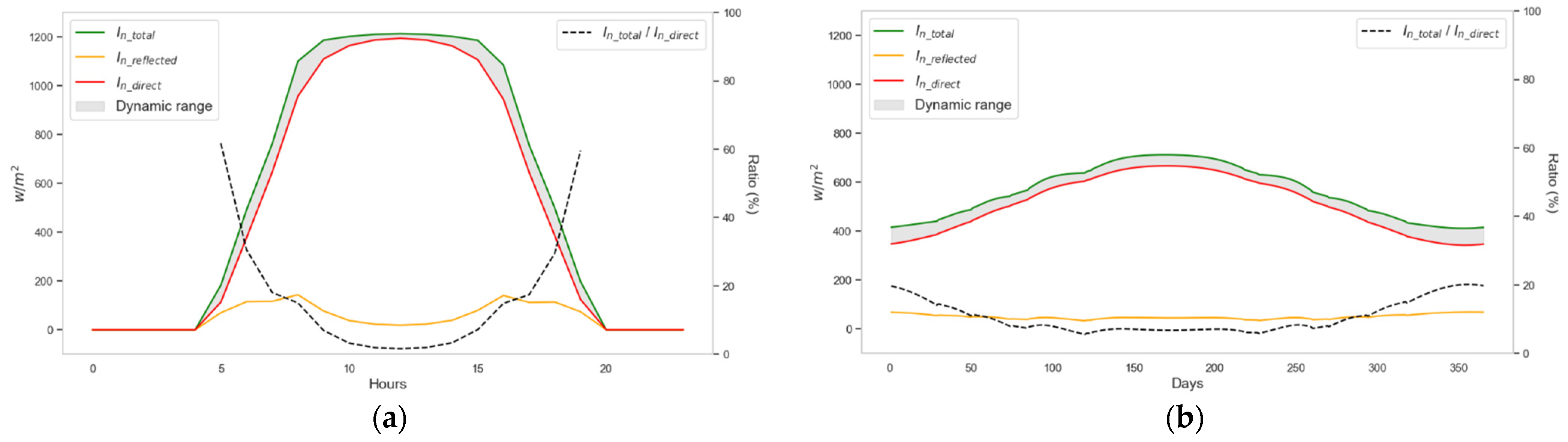
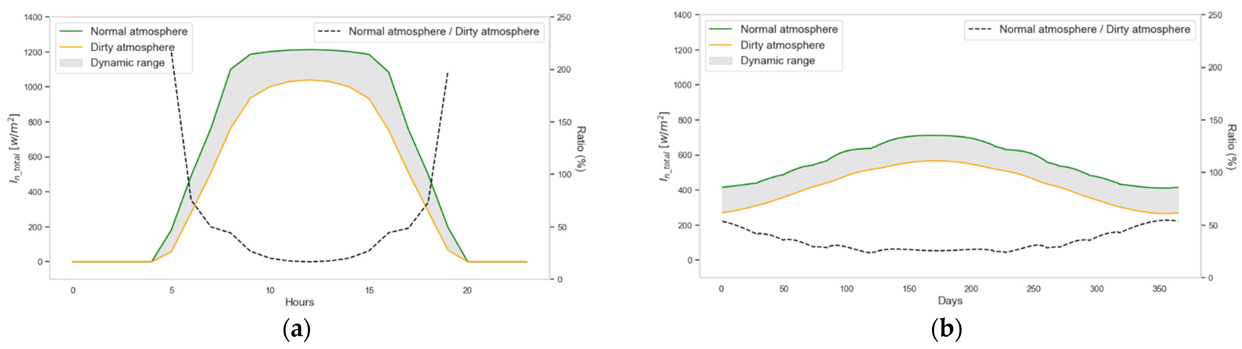
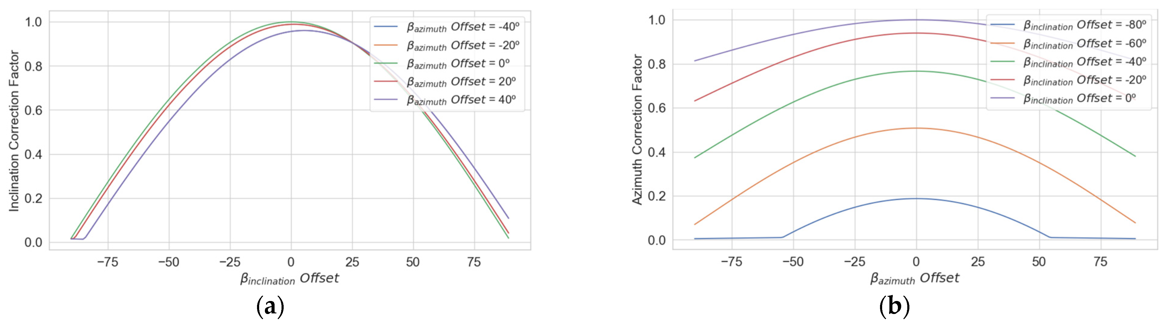
2.5.2. Modeling of Perpendicular Solar Radiation Received on the Surface of Photovoltaic Panels

Once the relative position of the sun is determined, it is possible to model the expected solar radiation density (${PV}_w$) received daily and perpendicularly on the surface of the photovoltaic panels (Equation (27)).

The first step in this process is to model the solar radiation density received at the upper boundary of the Earth’s atmosphere throughout each day of the year. The calculation of $I_{solar}$ was performed using the following expression [30]:

$$I_{solar}=1367\times (1+0.033\times cos(2\pi \times {\displaystyle \frac{ \mathrm{N}}{N_{days}}}\left)\right)$$

(14)

where 1367 W/m² is known as the solar constant (C_solar) and represents the density of received solar radiation.

As it passes through the Earth’s atmosphere, $I_{solar}$ is attenuated ($I_{attenuated}$) due to its angle of incidence (90 − ${\alpha }_{solar\_elevation}$), the path followed by the solar rays from the upper atmosphere to the point on the Earth’s surface where the solar panels are located—air mass ($M_{air}$)—and the state/quality of the atmosphere itself (K_i), where i depends on the different types of atmospheric absorption and scattering processes.

Kasten and Young [34] defined air mass ($M_{air}$) as the distance that $I_{solar}$ must travel from the upper boundary of the atmosphere to the terrestrial location of an observer—the location of the solar panels powering the green hydrogen station. According to Kasten and Young, $M_{air}$ can be modeled as follows:

$$M_{air}={\displaystyle \frac{1}{cos\left(\frac{2\pi }{360}\times (90-{\alpha }_{solar\_elevation})\right)+0.50572\times {\left(96.07995-(90-{\alpha }_{solar\_elevation})\right)}^{-1.6364}}}$$

(15)

Beer–Lambert [35,36] modeled the attenuation that $I_{solar}$ undergoes due to $M_{air}$ (Equation (15)) and atmospheric absorption and scattering processes (k_i).

Based on this, the solar radiation density (${\displaystyle \frac{\mathrm{w}}{{\mathrm{m}}^2}}$) received on a specific day of the year (Equation (14)), at a specific location on Earth (Equation (15)), and under specific atmospheric conditions (Equation (16)), is referred to as $I_{attenuated}$ and is modeled as follows:

$$I_{attenuated}=\left|(I_{solar}\times e^{-M_{air}\ast \left(K_a+K_g+K_{no2}+K_w+K_{o3}+K_r\right)})\right|$$

(16)

where k_i represents [37]:

• k_a: Attenuation due to aerosols.
• k_g: Attenuation due to gases (carbon dioxide and oxygen).
• k_NO2: Attenuation due to nitrogen dioxide.
• k_w: Attenuation due to water vapor.
• k_O3: Attenuation due to ozone layer.

In cases where the green hydrogen station is located offshore, the solar radiation density received on the surface of the photovoltaic panels is amplified due to the reflection of solar radiation on the marine surface.

Snell [33,38] modeled the calculation of the solar rays’ reflection angle (${\alpha }_{refraction}$) based on the air reflection coefficient [39] ($n_{air}$), the water reflection coefficient ($n_{water}$), and the incidence angle of the solar rays (${\alpha }_{incident}$) before impacting the marine surface:

$${\alpha }_{incident}={\displaystyle \frac{2\pi }{360}}\times (90-{\alpha }_{solar\_elevation})$$

(17)

$${\alpha }_{refraction}=arcsin({\displaystyle \frac{n_{air}}{n_{water}}}\times sin({\alpha }_{incident}\left)\right)$$

(18)

Fresnel [40,41] modeled the calculation of the power reflected on the sea surface ($I_{reflected}$) as the average of the coefficients rs and rp [32] ($k_{reflexion}$), which in turn are calculated based on the coefficients $n_{air}$, $n_{water}$, and the angles ${\alpha }_{incident}$ and ${\alpha }_{refraction}$. Fresnel’s law is modeled using the following expression:

$$\begin{gathered} rs={\left({\displaystyle \frac{n_{air}\times cos\left({\alpha }_{incident}\right)-n_{water}\times cos\left({\alpha }_{refraction}\right)}{n_{air}\times cos\left({\alpha }_{incident}\right)+n_{water}\times cos\left({\alpha }_{refraction}\right)}}\right)}^2 \\ rp={\left({\displaystyle \frac{n_{water}\times cos\left({\alpha }_{incident}\right)-n_{air}\times cos\left({\alpha }_{refraction}\right)}{n_{water}\times cos\left({\alpha }_{incident}{\alpha }_{incident}\right)+n_{air}\times cos\left({\alpha }_{refraction}\right)}}\right)}^2 \\ {k}_{reflextion}={\displaystyle \frac{rs+rp}{2}} \end{gathered}$$

(19)

In this way, the reflected solar radiation density is calculated by combining the results of expressions (Equations (16) and (19)):

$$I_{reflected}=I_{attenuated}\times k_{reflexion}$$

(20)

In any case, the previous expression (Equation (20)) assumes that the marine surface is completely flat, meaning that it has no irregularities that could affect the way solar rays are reflected. This assumption may be quite bold in marine environments, where the marine surface is subject to currents, winds, waves, or even the passage of ships that can create surface undulations, leading to a greater or lesser reduction in the actual value of $I_{reflected}$. This situation can be modeled by incorporating a loss coefficient ($K_{marine}$), which attenuates the original value of $I_{reflected}$. The values of $K_{marine}$ range within the interval [0, 1], where “0” represents the ideal condition of a perfectly flat marine surface, and “1” represents a completely irregular surface.

$$I_{reflected}=I_{reflected}\times (1-K_{marine})$$

(21)

At this point, the total solar radiation density ($I_{total}$) received on the surface of the panels is equal to the sum of the solar radiation densities: $I_{attenuated}$ (Equation (16)), $I_{reflected}$ (Equation (21)), and diffuse radiation ($I_{difused}$).

Throughout this paper, the value of $I_{difused}$ is zero, as this type of radiation depends on uncontrollable atmospheric conditions that are highly variable and difficult to model.

$$I_{total}=I_{attenuated}+I_{reflected}+I_{difused}$$

(22)

The sum of the solar radiation densities shown in expression (Equation (22)) is only possible after calculating their geometric contributions relative to the normal of the photovoltaic panel surface, both for direct solar radiation density ($K_{direct}$) and reflected radiation density ($K_{reflected}$). This condition is necessary due to the following: (i) the different incidence angles at which each type of radiation impacts the surface of the panels and (ii) the photovoltaic panels’ conversion capacity, which is specified based on the total solar radiation density received perpendicularly on their surface ($I_{n\_total}$), the surface area of the photovoltaic panels in square meters ($M_{panels}$), and the technological efficiency coefficient ($K_{panels}$). This last parameter is specified in the datasheets provided by the photovoltaic panel manufacturer.

Expression (Equation (23)) presents the geometric conversion factor necessary to normalize the direct solar radiation density (Equation (16)) impacting the panel surface ($K_{direct}$). This normalization depends on ${\alpha }_{solar\_elevation}$ (Equation (8)), ${\alpha }_{solar\_azimuth}$ (Equation (9)), the panel inclination angle relative to the ground (${\beta }_{inclination}$), and the panel azimuth angle (${\beta }_{azimuth}$) relative to the north or south, depending on the hemisphere in which the installation is located [30].

$$\begin{gathered} K_{direct}=sin\left({\alpha }_{solar\_elevation}\right) \ast sin\left({\beta }_{inclination}\right)+cos\left({\alpha }_{solar\_elevation}\right)\ast cos\left({\beta }_{inclination}\right) \\ \ast cos({\alpha }_{solar\_azimuth}-{\beta }_{azimuth}) \end{gathered}$$

(23)

In this way, the value of the direct and perpendicular solar radiation received on the panels’ surface ($I_{n\_direct}$) is modeled using the following expression:

$$I_{n\_direct}=I_{attenuated}\times K_{direct}$$

(24)

Symmetrically, expression (Equation (25)) presents the geometric conversion factor necessary to normalize the reflected solar radiation density (Equation (20)) impacting the panel surface ($K_{reflected}$). This normalization depends on ${\alpha }_{solar\_elevation}$ (Equation (8)), ${\alpha }_{solar\_azimuth}$ (Equation (9)), the panel inclination angle relative to the ground (${\beta }_{inclination}$), and the panel azimuth angle (${\beta }_{azimuth}$) relative to the north or south, depending on the hemisphere where the installation is located:

$$\begin{gathered} K_{reflected}=sin(-{\alpha }_{solar\_elevation})\times sin\left({\beta }_{inclination}\right) \\ +cos(-{\alpha }_{solar\_elevation})\times cos\left({\beta }_{inclination}\right)\times cos({\alpha }_{solar\_azimuth}-{\beta }_{azimuth}) \end{gathered}$$

(25)

In this way, the value of the reflected and perpendicular solar radiation received on the panels’ surface ($I_{n\_reflected}$) is modeled using the following expression:

$$I_{n\_reflected}=I_{reflected} \times K_{reflected}$$

(26)

Using expressions (Equations (24) and (26)), and considering that the value of $I_{difused}$ is equal to zero, the expression for $I_{total}$ (Equation (22)) can be reformulated to calculate the total solar radiation density received perpendicularly on the photovoltaic panels ($I_{n\_total}$):

$$I_{n\_total}=I_{n\_direct}+I_{n\_reflected}$$

(27)

At this point, knowing $I_{n\_total}$, considering the photovoltaic panels’ capacity to convert solar radiation density per square meter ($K_{panels}$), and the available panel surface area ($M_{panels}$), the total calculation of the electrical power generated by the photovoltaic panels (${PV}_w$) is modeled as follows:

$${PV}_w=I_{n\_total}\times K_{panels}\times M_{panels}$$

(28)

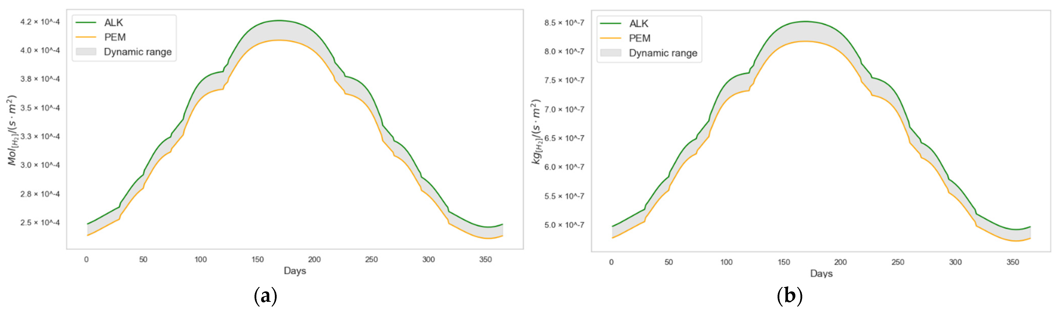
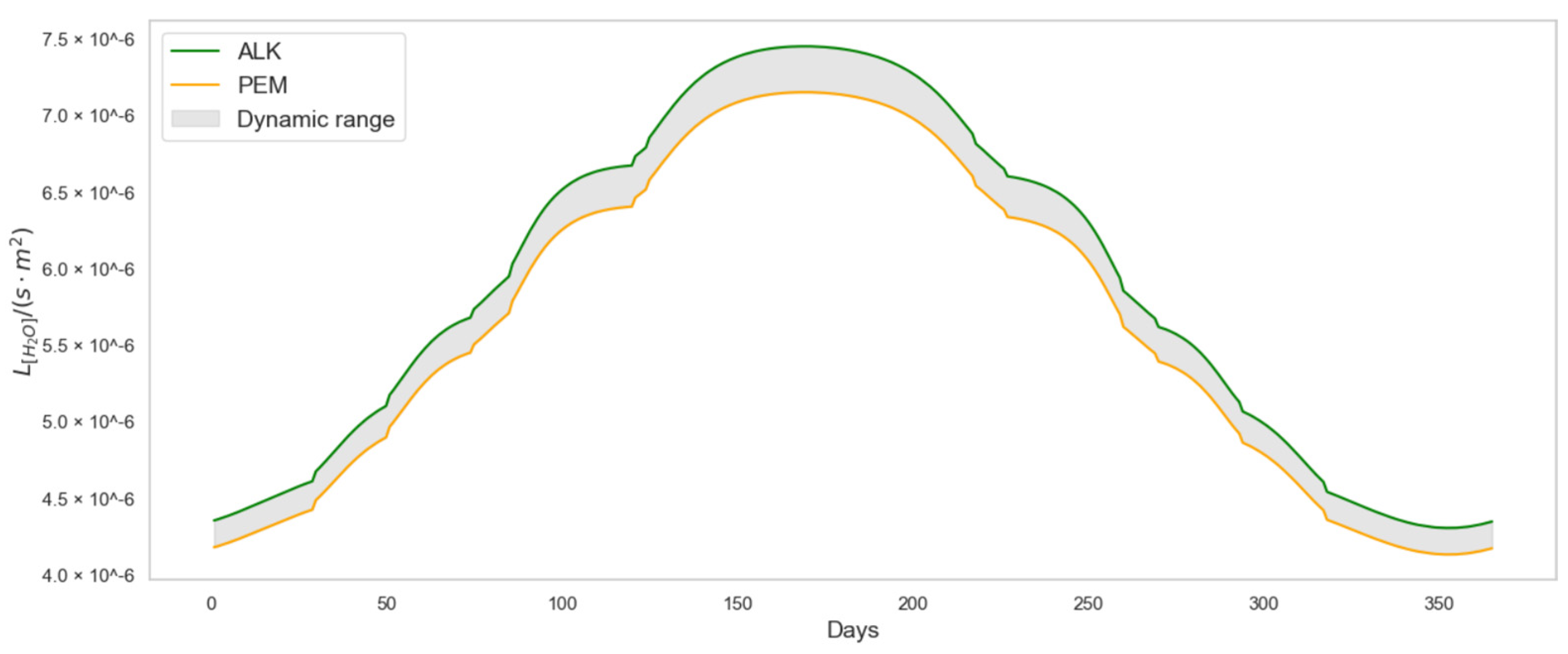
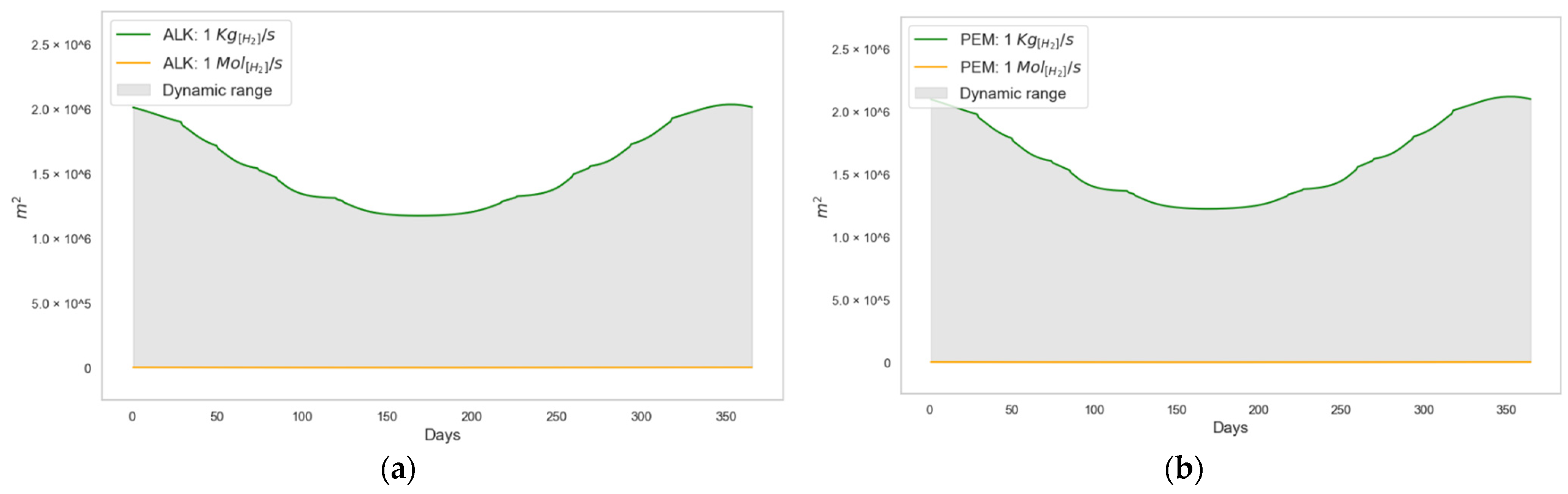
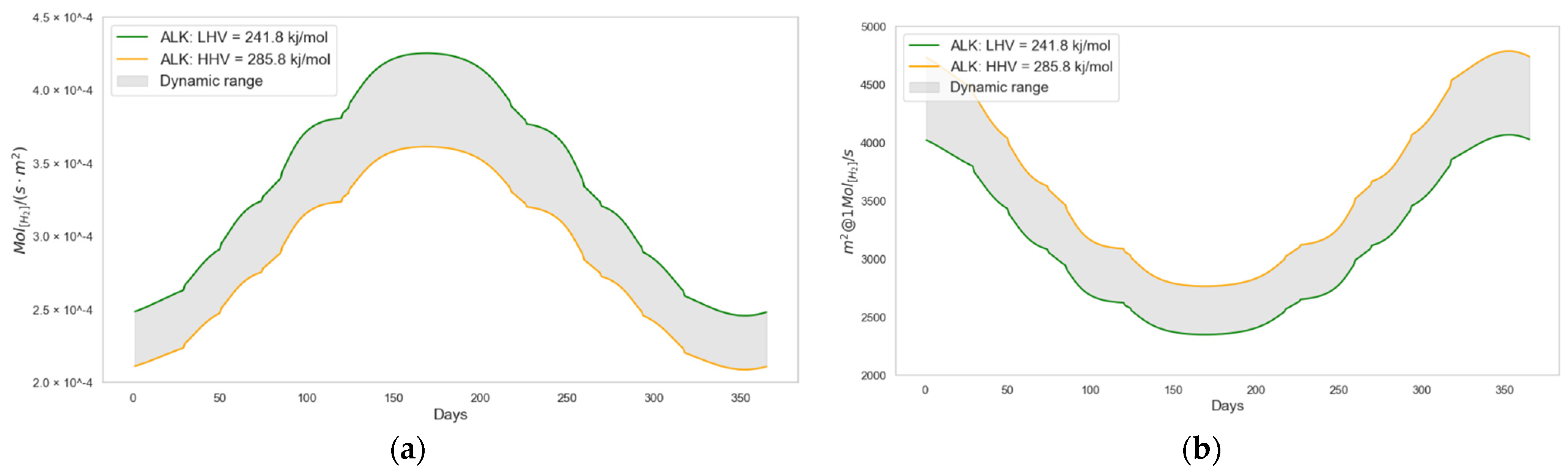
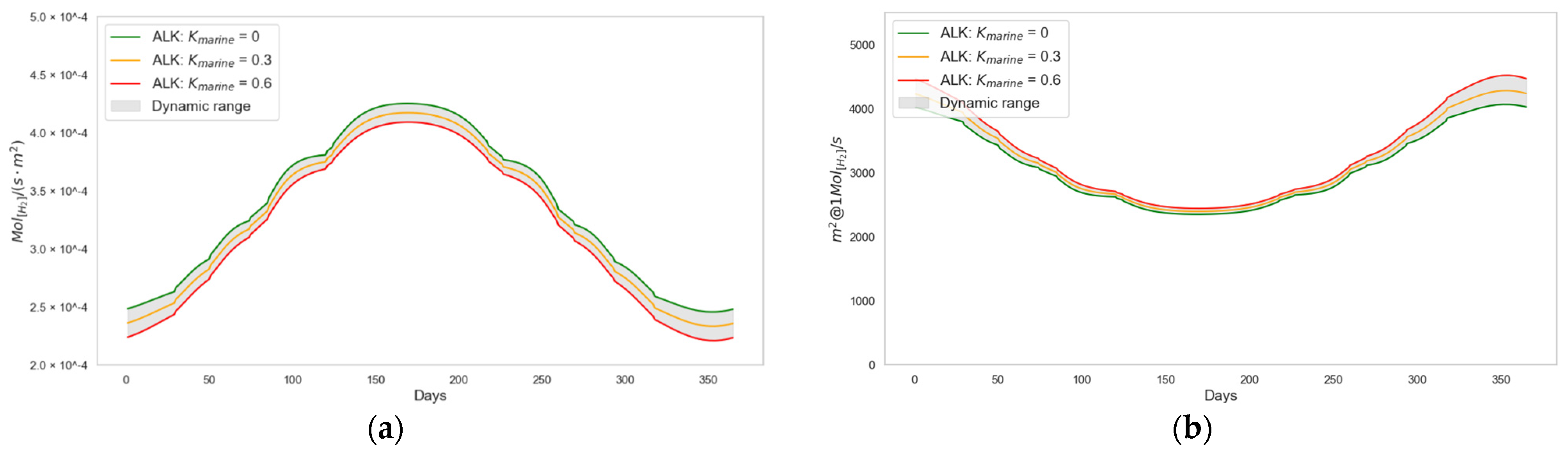
2.6. PHASE III: Modeling of an Electrolyzer: Type ALK and PEM

The mathematics-based technical model used to estimate the energy consumption required to produce a given number of ${\displaystyle \frac{\mathrm{m}\mathrm{o}\mathrm{l}}{\mathrm{s}}}$ of hydrogen ($N_{mol}$) through the dissociation of the hydrogen molecule—water electrolysis—is expressed as (${PW}_i$) (Equation (29)).

The value of the hydrogen heating value constant (HV) depends on the design of the green hydrogen station and its energy recovery capacity. Therefore, the electrolyzer model allows for the use of both the higher heating value of hydrogen (HHV = 285.8 ${\displaystyle \frac{\mathrm{k}\mathrm{J}}{\mathrm{m}\mathrm{o}\mathrm{l}}}$) and the lower heating value (LHV = 241.8 ${\displaystyle \frac{\mathrm{k}\mathrm{J}}{\mathrm{m}\mathrm{o}\mathrm{l}}}$). The actual efficiency of the electrolyzer is modeled by dividing the theoretical calculation by an efficiency coefficient that depends on the model and type of electrolyzer selected ($K_{electrolyzer\_i}$). In both cases, i represents the type of technology used in the electrolyzer—ALK or PEM. The electrolyzer’s energy consumption is expressed in ${\displaystyle \frac{\mathrm{k}\mathrm{J}}{\mathrm{s}}}$ or $\mathrm{k}\mathrm{w}$.

$${PW}_i={\displaystyle \frac{N_{mol}\times HV }{K_{electrolyzer\_i}}}$$

(29)

According to recently published ALK and PEM electrolyzer models [42], the authors estimate the value of $K_{electrolyzer\_i}$ (Equations (30) and (31)) based on the commissioning year of the station, respectively.

$$K_{electrolyzer\_ALK}={\displaystyle \frac{1}{(555.25-0.25\times year)}}$$

(30)

$$K_{electrolyzer\_PEM}={\displaystyle \frac{1}{(1570.75-0.75\times year)}}$$

(31)

As part of the model presented in this article, equations (Equations (30) and (31)) were used to determine the relationship between the efficiencies associated with each type of electrolyzer ($R_{ALK\_PEM}$):

$$R_{ALK\_PEM}={\displaystyle \frac{K_{electrolyzer\_ALK}}{K_{electrolyzer\_PEM}}}={\displaystyle \frac{(1570.75-0.75\times year)}{(555.25-0.25\times year)}}$$

(32)

Additionally, in the same article [43], the authors also present two other mathematical models to characterize the relationship between the commissioning year of the station (year) and the hydrogen pressure at the output of each type of electrolyzer.

In this way, the model was obtained for the ALK electrolyzer type ($P_{ALK}$) (Equation (33)) and for the PEM electrolyzer type ($P_{PEM}$) (Equation (34)). Both results are expressed in bar.

$$P_{ALK}=-3528.75+1.75\times year$$

(33)

$$P_{PEM}=-7533.75+3.75\times year$$

(34)

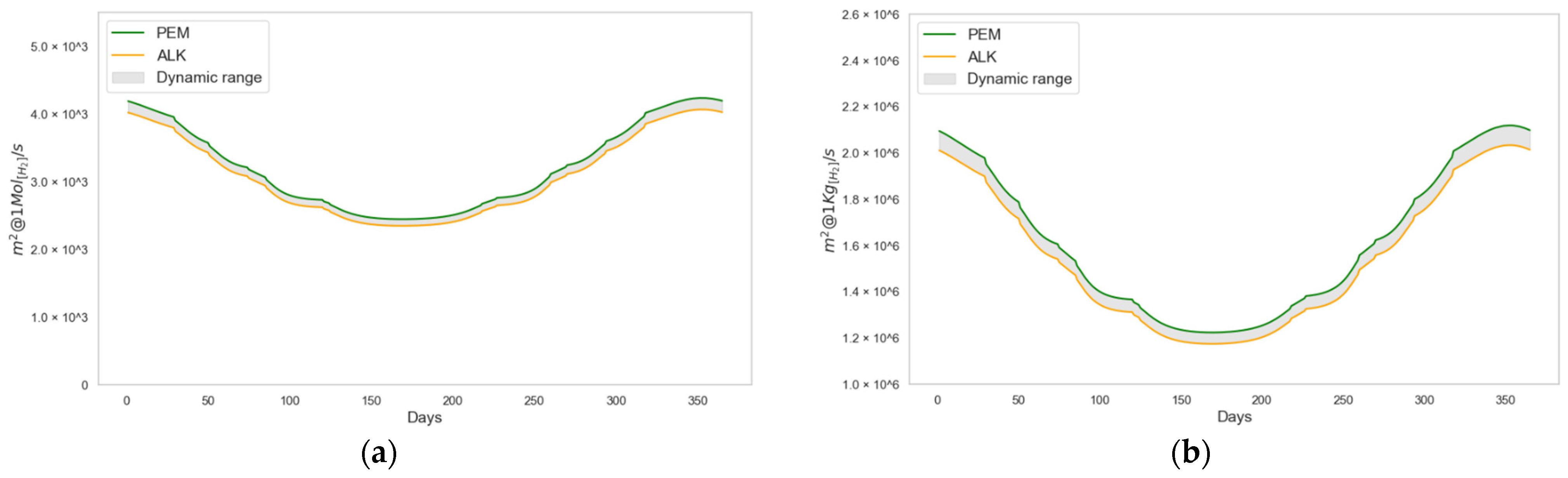
2.7. PHASE IV: Modeling of an Adiabatic Compressor

The estimated energy consumption for an adiabatic compressor (${PW}_{COM}$), used to compress the green hydrogen produced by an electrolyzer—regardless of its technology type—is modeled using expression (Equation (35)), with results expressed in ${\displaystyle \frac{\mathrm{J}}{\mathrm{s}}}$ or $\mathrm{w}$.

This expression establishes the relationship between ${PW}_{COM}$ and the input parameters: $N_{mol}$, the ideal gas constant (R), expressed in ${\displaystyle \frac{\mathrm{J}}{\mathrm{m}\mathrm{o}\mathrm{l}·\mathrm{K}}}$; the inlet ($T_{in}$) and outlet ($T_{out}$) temperatures, expressed in Kelvin; the compressor efficiency coefficient ($K_{compressor}$); and the adiabatic constant of hydrogen (Y).

$${PW}_{COM}=\left|{\displaystyle \frac{N_{mol}\times R\times (T_{out}-T_{in})}{K_{compressor}\times (1-Y)}}\right|$$

(35)

The theoretical value of $T_{out}$ is calculated based on $T_{in}$, Y, the inlet pressure of the compressor, equal to the electrolyzer’s output pressure ($P_{in}$), and the outlet pressure ($P_{out}$), which corresponds to the hydrogen storage pressure (Equation (36)). This calculation can also be performed based on the hydrogen volumes at the compressor’s inlet ($V_{in}$) and outlet ($V_{out}$) (Equation (37)).

$$T_{out}=T_{in}\times {\displaystyle \frac{{P_{out}}^{\frac{Y-1}{Y}}}{P_{in}}}$$

(36)

$$T_{out}=T_{in}\times {\displaystyle \frac{{V_{in}}^{Y-1}}{V_{out}}}$$

(37)

where $V_{in}$ is calculated using the ideal gas equation:

$$V_{in}={\displaystyle \frac{N_{mol}\times R\times T_{in}}{P_{in}}}$$

(38)

and $V_{out}$ (Equation (40)) is calculated using the relationship between pressure (P) and volume (V) in the adiabatic process. This relationship remains constant (C) and follows an exponential dependence on Y (Equation (39)).

$$C=P\times V^Y$$

(39)

$$V_{out}={\displaystyle \frac{V_{in}}{e^{\frac{ln\left(\frac{P_{out}}{P_{in}}\right)}{Y}}}}$$

(40)

2.8. PHASE V: Integration of All Components into a Cohesive System

Once $N_{mol}$, $P_{out}$, and the electrolyzer technology type—ALK or PEM—are defined, it is possible to estimate the total energy consumption required for the green hydrogen production and compression processes (${PW}_{Total\_i}$), where i represents the type of technology used by the electrolyzer. This energy consumption, expressed in ${\displaystyle \frac{\mathrm{k}\mathrm{J}}{\mathrm{s}}}$ or $\mathrm{k}\mathrm{w}$, is calculated as the sum of the individual consumption of the electrolyzer and the compressor (Equation (41)):

$${PW}_{Total\_i}={PW}_i+{\displaystyle \frac{{PW}_{COM}}{{10}^3}}$$

(41)

It is also possible to size the photovoltaic station so that the entire green hydrogen production and compression process can be continuously and sustainably powered by solar energy (Equation (41)). To achieve this, the expression for photovoltaic panel electricity generation capacity (Equation (28)) was set equal to the expression for total energy consumption (Equation (41)), allowing for the calculation of the required photovoltaic panel surface area ($M_{panels}$) needed to power the entire station (Equation (42)) and maintain the energy balance. Here, $M_{panels}$ is expressed in square meters (m²).

$$M_{panels}={\displaystyle \frac{{PW}_{Total\_i}\times {10}^3}{I_{n\_total}\times K_{panels}}}$$

(42)

Although equation (Equation (42)) allows for calculating the required photovoltaic panel surface area to implement a green hydrogen station that operates at a specific location (Equation (1)), for a given hydrogen flow rate (${\displaystyle \frac{\mathrm{m}\mathrm{o}\mathrm{l}}{\mathrm{s}}}$) and at a defined output pressure ($P_{out}$), it is recommended to determine the contribution of each unit of panel surface area (1 m²) to the amount of hydrogen produced and stored by the station. To achieve this, equation (Equation (42)) is expanded and expressed in terms of ${\displaystyle \frac{\mathrm{m}\mathrm{o}\mathrm{l}}{\mathrm{s}\times {\mathrm{m}}^2}}$:

$${\displaystyle \frac{\mathrm{m}\mathrm{o}\mathrm{l}}{\mathrm{s}\times {\mathrm{m}}^2}}={\displaystyle \frac{I_{n\_total}\times K_{panels}}{\frac{HV}{K_{electrolyzer\_i}}\times 1000+\left|\frac{R \times (T_{out}-T_{in})}{K_{compressor}\times (1-Y)}\right| }}$$

(43)

As can be observed, the numerator represents the photovoltaic station’s electricity generation capacity per square meter of surface area, while the denominator represents the electrical consumption required for the production and storage of 1 ${\displaystyle \frac{\mathrm{m}\mathrm{o}\mathrm{l}}{\mathrm{s}}}$ of hydrogen. Considering that the theoretical molecular mass of hydrogen ($m_{h2}$) is a constant with a value of 2 × ${10}^{-3} {\displaystyle \frac{\mathrm{k}\mathrm{g}}{\mathrm{m}\mathrm{o}\mathrm{l}}}$, equation (Equation (43)) can be expressed in terms of the ${\displaystyle \frac{\mathrm{k}\mathrm{g}}{\mathrm{s}}}$ of hydrogen produced and stored per square meter of panel surface area:

$${\displaystyle \frac{\mathrm{k}\mathrm{g}}{\mathrm{s}\times {\mathrm{m}}^2}}=\left({\displaystyle \frac{\mathrm{m}\mathrm{o}\mathrm{l}}{\mathrm{s}\times {\mathrm{m}}^2}}\right)\times m_{h2}$$

(44)

Green hydrogen production is achieved by dissociating the water molecule (H₂O) through the process known as electrolysis, consuming one mole of water for every mole of hydrogen produced. Based on this relationship, using equation (Equation (43)) and considering that the molecular mass of water ($m_{h20}$) is equal to 18 ×${10}^{-3} {\displaystyle \frac{\mathrm{k}\mathrm{g}}{\mathrm{m}\mathrm{o}\mathrm{l}}}$ and that the density of seawater (${\rho }_{h20}$) is approximately 1.02819 ${\displaystyle \frac{\mathrm{k}\mathrm{g}}{\mathrm{l}}}$, the estimation of the water flow required at the station’s inlet (${\displaystyle \frac{\mathrm{l}}{\mathrm{s}\mathrm{e}\mathrm{c}}}$), for the production of a given number of ${\displaystyle \frac{\mathrm{m}\mathrm{o}\mathrm{l}}{\mathrm{s}}}$ of hydrogen, and as a function of the available photovoltaic panel surface area (m²), can be calculated as follows:

$${\displaystyle \frac{\mathrm{l}}{\mathrm{s}\times {\mathrm{m}}^2}}={\displaystyle \frac{\left(\frac{\mathrm{m}\mathrm{o}\mathrm{l}}{\mathrm{s} \times {\mathrm{m}}^2}\right)\times m_{h20}}{{\rho }_{h20}}}$$

(45)

By isolating the photovoltaic panel surface area in equation (Equation (43)), the required number of square meters (m²) needed for the production of 1 ${\displaystyle \frac{\mathrm{m}\mathrm{o}\mathrm{l}}{\mathrm{s}}}$ of hydrogen is obtained:

$${\mathrm{m}}^2=(1 {\displaystyle \frac{\mathrm{m}\mathrm{o}\mathrm{l}}{\mathrm{s}}})\times {\displaystyle \frac{\frac{HV}{K_{electrolyzer\_i}}\ast 1000+\left|\frac{R \times (T_{out}-T_{in})}{K_{compressor} \times (1-Y)}\right| }{I_{n\_total}\times K_{panels}}}$$

(46)

Similarly, by isolating the photovoltaic panel surface area in equation (Equation (44)), the required number of square meters (m²) needed to produce 1 ${\displaystyle \frac{\mathrm{k}\mathrm{g}}{\mathrm{s}}}$ of hydrogen is obtained:

$${\mathrm{m}}^2=(1 {\displaystyle \frac{\mathrm{k}\mathrm{g}}{\mathrm{s} }})\times {\displaystyle \frac{1}{\left(\frac{\mathrm{m}\mathrm{o}\mathrm{l}}{\mathrm{s} \times {\mathrm{m}}^2}\right)\times m_{h2}}}$$

(47)

Likewise, by isolating the photovoltaic panel surface area in equation (Equation (45)), the required number of square meters (m²) needed for the consumption of 1 ${\displaystyle \frac{\mathrm{l}}{\mathrm{s}}}$ of H₂O is obtained:

$${\mathrm{m}}^2=(1 {\displaystyle \frac{\mathrm{l}}{\mathrm{s} }})\times {\displaystyle \frac{{\rho }_{h20}}{\left(\frac{\mathrm{m}\mathrm{o}\mathrm{l}}{\mathrm{s} \times {\mathrm{m}}^2}\right)\times m_{h20}}}$$

(48)

Expressions (Equations (46)–(48)) can be used as comparative elements for different locations, green hydrogen production, and compression technologies. Thus, for the same amount of hydrogen produced (${\displaystyle \frac{\mathrm{m}\mathrm{o}\mathrm{l}}{\mathrm{s}}}$, ${\displaystyle \frac{\mathrm{k}\mathrm{g}}{\mathrm{s}}}$) and stored at the same output pressure ($P_{out}$), the most efficient location and green hydrogen station will be the one that achieves these values using the least photovoltaic panel surface area (m²). In other words, the station that requires lower energy consumption will be more efficient. The higher the efficiency of the green hydrogen station, the lower the associated costs related to installation, commissioning, and maintenance throughout its operational lifetime.

3. Results

As part of the results presented in this paper, the previously described mathematics-based technical model is adapted and applied to a case study involving a green hydrogen production station powered by solar energy, intended to be installed in the town of Santoña (Cantabria, Spain). This site is an ideal location for testing marine energy prototypes due to several key characteristics. Firstly, its location on the Cantabrian coast provides direct access to the open sea (Figure 4). Secondly, the Santoña Bay, covering an area of 28 km², offers a protected yet representative environment for conducting initial testing [42]. Lastly, the presence of the “Parque Natural de las Marismas de Santoña y Noja” highlights the importance of developing environmentally friendly energy technologies in the region [44].

With the objective of calculating the average level of $I_{n\_total}$ received on the photovoltaic panels, the following model parameters are configured and summarized in

Table 2. Case-specific configuration of mathematics-based technical model parameters: location, time definition, atmospheric and marine conditions, and photovoltaic panels.

Parameter	Value
GPS position of the installation:	Santoña, Spain
Year under study (year):	2025
$\mathrm{Total} \mathrm{number} \mathrm{of} \mathrm{days} \mathrm{in} \mathrm{the} \mathrm{year} (N_{days}$):	365
Day of the year under study (N):	All
$\mathrm{Local} \mathrm{time} (h_{local}$):	All
Atmospheric state/quality:	Normal
$\mathrm{Radiation} \mathrm{losses} \mathrm{due} \mathrm{to} \mathrm{marine} \mathrm{surface} \mathrm{irregularities} (K_{marine}$):	0
Panel inclination and azimuth relative to the sun’s position (${\beta }_{inclination}$) and (${\beta }_{azimuth}$):	Perfect alignment with the estimated sun position
$\mathrm{Photovoltaic} \mathrm{panel} \mathrm{conversion} \mathrm{efficiency} (K_{panels}$):	0.2

: location, time definition, atmospheric and marine conditions, and photovoltaic panels input parameters.

Once these input parameters are configured and the technical model is executed in Python, the results include the estimations of the following variables: ${\displaystyle \frac{{\mathrm{m}\mathrm{o}\mathrm{l}}_{{\mathrm{H}}_2}}{\mathrm{s}\times {\mathrm{m}}^2}}$ (Equation (43)), ${\displaystyle \frac{{\mathrm{k}\mathrm{g}}_{{\mathrm{H}}_2}}{\mathrm{s}\times {\mathrm{m}}^2}}$ (Equation (44)), and ${\displaystyle \frac{{\mathrm{l}}_{{\mathrm{H}}_{2}0}}{\mathrm{s}\times {\mathrm{m}}^2}}$ (Equation (45)), as well as the photovoltaic panel surface area required for the production of $1 {\displaystyle \frac{{\mathrm{m}\mathrm{o}\mathrm{l}}_{{\mathrm{H}}_2}}{\mathrm{s}}}$ (Equation (46)) and $1 {\displaystyle \frac{{\mathrm{k}\mathrm{g}}_{{\mathrm{H}}_2}}{\mathrm{s}}}$ (Equation (47)), and the consumption of $1 {\displaystyle \frac{{\mathrm{l}}_{{\mathrm{H}}_{2}0}}{\mathrm{s}}}$ (Equation (48)).

Figure 5 presents the average value of $I_{n\_total}$ (Equation (27)), calculated for all hours of the day (a) and for all days of the year (b). Using the average value simplifies the analysis and sizing of the station, allowing it to be conducted from a statistical perspective. However, the technical model of the station also enables the calculation of the estimated natural values of $I_{n\_total}$ for each hour of the day and each day of the year.

Figure 5a illustrates that the average levels of $I_{n\_total}$ are equal to 0 during the hours of the day when ${\alpha }_{solar\_elevation}$ (Equation (8)) is either 0 or negative and greater than 0 when ${\alpha }_{solar\_elevation}$ is positive. The maximum value is reached when ${\alpha }_{solar\_elevation}$ is also at its highest within the same day. This occurs at 12 p.m. local time.

Figure 5b shows the influence of the hours without solar radiation (nighttime). As a result, the obtained values exhibit a smoother evolution compared to Figure 5a. Since it represents an average of the total solar radiation density received throughout the day, its minimum value is always greater than 0. The maximum daily average value is reached when ${\alpha }_{solar\_elevation}$ is at its highest throughout the different days of the year, which occurs during the local summer months.

However, in both Figure 5a,b, it can be observed that the average density of reflected solar radiation, $I_{n\_reflected}$, reaches its minimum when ${\alpha }_{solar\_elevation}$ is at its maximum, at 12 p.m. This situation can be explained by considering that, according to Snell’s law, $I_{n\_reflected}$ depends on ${\alpha }_{incident}$, which increases when ${\alpha }_{solar\_elevation}$ is lower, at sunrise and sunset. As expressed in equation (Equation (27)), the total radiation density ($I_{n\_total}$) is the sum of direct radiation ($I_{n\_direct}$) and reflected radiation ($I_{n\_reflected}$). The contribution $I_{n\_reflected}$ becomes more significant during periods of low ${\alpha }_{solar\_elevation}$. In the case under analysis, the contribution of $I_{n\_reflected}$ leads to an average increase of 18.2% in the $I_{n\_total}$ received—when averaged over the hours of a typical day—and 10.54% when averaged over the days of the year. A vertical axis of symmetry is observed in both Figure 5a,b, centered around the position of the maximum value.

The subsequent step in the mathematics-driven analysis process involves estimating the average energy consumption of the station’s electrolyzer and adiabatic compressor. (Equation (41)). To this end, it is necessary to configure the model input parameters related to the electrolyzer and the adiabatic compressor, which are summarized in

Table 3. Case-specific configuration of mathematics-based technical model parameters: electrolyzers and adiabatic compressor.

Parameter	Value
$\mathrm{Number} \mathrm{of} \mathrm{moles} (N_{mol}$):	1
Electrolyzer type (i):	ALK, PEM
Selected heating value constant (HV):	LHV
$\mathrm{Conversion} \mathrm{efficiency} \mathrm{of} \mathrm{both} \mathrm{electrolyzer} \mathrm{types} (K_{electrolyzer\_i}$):	PEM = 0.7 $K_{electrolyze{r}_{ALK}}$$=K_{electrolyze{r}_{PEM}}\times R_{ALK\_PEM}$ (Equation (32))
$\mathrm{Compressor} \mathrm{efficiency} (K_{compressor}$):	0.7
$\mathrm{Operating} \mathrm{ambient} \mathrm{temperature} (T_{in}$):	12.5 °C
$\mathrm{Compressor} \mathrm{inlet} \mathrm{pressure} (\mathrm{dependent} \mathrm{on} \mathrm{electrolyzer} \mathrm{type}) (P_{in}$):	According to electrolyzer type and year (Equations (33) and (34))
$\mathrm{Compressor} \mathrm{outlet} \mathrm{pressure} (P_{out}$):	200 bars

.

In this way, the produced and stored hydrogen flow rate (${\displaystyle \frac{{\mathrm{m}\mathrm{o}\mathrm{l}}_{{\mathrm{H}}_2}}{\mathrm{s}\times {\mathrm{m}}^2}}$) and (${\displaystyle \frac{{\mathrm{k}\mathrm{g}}_{{\mathrm{H}}_2}}{\mathrm{s}\times {\mathrm{m}}^2}}$), as well as the amount of water consumed (${\displaystyle \frac{{\mathrm{l}}_{{\mathrm{H}}_{2}0}}{\mathrm{s}\times {\mathrm{m}}^2}}$), are obtained. Figure 6a,b present the results represented in a day–year format. Additionally, the results for both electrolyzer models are included. Depending on the relationship $R_{ALK\_PEM}$ and the pressures $P_{ALK}$ and $P_{PEM}$, different outcomes are obtained.

As observed in all the graphs in Figure 6, the maximum values obtained using the PEM electrolyzer are slightly lower than those obtained with the ALK electrolyzer simulation conducted for the year 2025. In any case, as previously mentioned, the relationship $R_{ALK\_PEM}$ is a parameter dependent on the year (year) in which this study is conducted. In the case under study, the superior performance of ALK technology over PEM—quantified using the $R_{ALK\_PEM}$ ratio applicable to the year 2025—results in a 4.19% increase in the green hydrogen output rate, expressed in both ${\displaystyle \frac{{\mathrm{m}\mathrm{o}\mathrm{l}}_{{\mathrm{H}}_2}}{\mathrm{s}\times {\mathrm{m}}^2}}$ and ${\displaystyle \frac{{\mathrm{k}\mathrm{g}}_{{\mathrm{H}}_2}}{\mathrm{s}\times {\mathrm{m}}^2}}$, for an equivalent level of received total $I_{n\_total}$. This performance difference between the two technologies is expected to diminish over time as their respective efficiencies progressively converge.

Figure 7 shows the amount of water (l) consumed per second (s) in relation to the available solar panel surface area, expressed in square meters (m²). The 4.19% increase in green hydrogen production is proportionally reflected in the amount of water required at the input of the electrolyzer.

The average photovoltaic panel surface area required to produce 1 ${\displaystyle \frac{{\mathrm{m}\mathrm{o}\mathrm{l}}_{{\mathrm{H}}_2}}{\mathrm{s}}}$ and 1 ${\displaystyle \frac{{\mathrm{k}\mathrm{g}}_{{\mathrm{H}}_2}}{\mathrm{s}}}$ is represented in Figure 8, expressed in a day–year format. As observed, the estimated average photovoltaic panel surface area decreases when the levels of received solar radiation density (Figure 8a) and electrolyzer efficiencies are higher and vice versa. The graphs exhibit vertical symmetry centered at the points of the minimum surface area, which coincide with the points where ${\alpha }_{solar\_elevation}$ reaches its maximum value, and, consequently, so does the received solar radiation density. According to the relationship $R_{ALK\_PEM}$, the estimation for the year 2025 (Figure 8b) suggests that the ALK electrolyzer will be more efficient than the PEM electrolyzer. As a result, this improvement will lead to lower energy consumption and a smaller required panel surface area for the same hydrogen production capacity. In the case under analysis, this reduction in photovoltaic surface area corresponds to a 4.03% decrease. These differences will gradually diminish as PEM technology improves its efficiency relative to ALK. Regardless of the scenario, the continuous improvement of electrolyzer technology is vital, as increased efficiency directly contributes to lower energy consumption and a corresponding reduction in the required photovoltaic surface area.

Figure 9a presents the aggregation of the panel surface areas obtained in Figure 8a,b for both types of electrolyzers. This facilitates the comparison process by allowing an analysis of the required surface area values for each of the represented variables, considering their orders of magnitude. On the other hand, Figure 9b shows that the production of 1 ${\displaystyle \frac{{\mathrm{k}\mathrm{g}}_{{\mathrm{H}}_2}}{\mathrm{s}}}$ requires a larger panel surface area (due to higher energy consumption) compared to the case of 1 ${\displaystyle \frac{{\mathrm{m}\mathrm{o}\mathrm{l}}_{{\mathrm{H}}_2}}{\mathrm{s}}}.$ In the case under analysis, this ratio is equal to 500.

4. Discussion

This section discusses and justifies the proposed mathematics-based technical model used to model a green hydrogen production station powered by solar energy. To this end, a series of simulations and multivariable parametric analyses have been carried out to evaluate the model’s output behavior as a function of its input configuration parameters. From a logical standpoint, as detailed in the high-level flow diagram shown in Figure 2 and in each of its associated phases, the model can predict the solar trajectory based on the station’s geographic location, the day of the year, and the local time (Figure 10). Subsequently, the model estimates the total solar radiation, $I_{n\_total}$, received on the photovoltaic panels’ surface, considering the date and local time, the sun’s position and path, the geographic and physical orientation of the photovoltaic panels used to power the hydrogen station, and the atmospheric attenuation experienced by solar radiation before reaching the Earth’s surface (Figure 11). Finally, and equally important, the influence of the configuration parameters on the green hydrogen production rate at the station’s output is also analyzed. This output is expressed as ${\displaystyle \frac{{\mathrm{m}\mathrm{o}\mathrm{l}}_{{\mathrm{H}}_2}}{\mathrm{s}\times {\mathrm{m}}^2}}$, along with the required photovoltaic panel surface area (m²) to produce $1 {\displaystyle \frac{{\mathrm{m}\mathrm{o}\mathrm{l}}_{{\mathrm{H}}_2}}{\mathrm{s}}}$ of hydrogen. The equivalent hydrogen production values, expressed in ${\displaystyle \frac{{\mathrm{k}\mathrm{g}}_{{\mathrm{H}}_2}}{\mathrm{s}\times {\mathrm{m}}^2}}$ and ${\displaystyle \frac{{\mathrm{k}\mathrm{g}}_{{\mathrm{H}}_2}}{\mathrm{s}}}$, can be directly obtained by applying the expression (Equation (44)).

It is important to emphasize that the selection of parameter values will depend entirely on the specific case study being addressed. These values may be fixed or variable, measured or estimated, and may represent average, maximum, and/or minimum conditions—used to model input uncertainty and to analyze its impact on the output of the technical model representing the green hydrogen station powered by solar energy. In any case, for a given green hydrogen production requirement, the primary objective will be to minimize the surface area of the photovoltaic panels required to meet that demand. Logically, a smaller photovoltaic surface area simplifies the design and reduces the amount of material needed for the construction of the mechanical support structure—whether floating or fixed. A smaller panel surface area also proportionally decreases the forces exerted by wind and waves on the structure. As a result, a more compact station with reduced external loads facilitates simpler installation and anchoring processes while also decreasing the total amount and surface exposure of materials in contact with seawater. This, in turn, inevitably contributes to a reduction in the Levelized Cost of Electricity (LCOE) [19,25], as it simplifies the installation, operation, and maintenance processes of the entire system.

4.1. Solar Trajectory

One of the fundamental aspects of ensuring that the model accurately simulates the solar trajectory relative to the installation site is evaluating its ability to compute ${\alpha }_{solar\_elevation}$ and ${\alpha }_{solar\_azimuth}$, as well as the corrected solar angle using the general equation of solar time (${\alpha }_{solar\_corrected}$) (Equation (7)).

The sun, when observed at the same time of day from the same location throughout the year (year), traces an approximately figure-eight-shaped curve in the sky [45]. This curve is commonly known as the solar analemma. Figure 10 demonstrates the technical model’s capability to calculate the solar analemmas for each hour of the day, as seen from the location of the green hydrogen station and photovoltaic panels.

Where in black, the solar analemma corresponding to 12 p.m. local time is shown in the central area, representing the time of maximum solar elevation for each day of the year. In blue, the solar analemmas visible from the station’s location are represented, where ${\alpha }_{solar\_elevation}$ values are greater than 0 (daytime). In red, the solar analemmas correspond to negative ${\alpha }_{solar\_elevation}$ values, indicating that the Sun is below the horizon (nighttime).

4.2. Solar Irradiation and Green Hydrogen Station Capacity

In Figure 4, the normal solar radiation density received on the surface of the photovoltaic panels is represented, both in its direct component ($I_{n\_direct}$) and reflected component ($I_{n\_reflected}$), as well as the resulting total contribution ($I_{n\_total}$).

However, as described in expressions (Equations (15) and (16)), the radiation density received at the Earth’s surface is attenuated by the effects of $M_{air}$ and atmospheric conditions such as those resulting from absorption and scattering processes [46]. These processes define the atmospheric quality between the Sun’s position and the photovoltaic station. Figure 11 illustrates the effect of atmospheric attenuation on $I_{n\_total}$ values received on the panel surfaces. Lower atmospheric quality leads to higher attenuation (higher absorption and scattering coefficients), resulting in lower $I_{n\_total}$ values. In the case under analysis, the average attenuation of the total irradiance $I_{n\_total}$ received by the photovoltaic panels is 31.16% when averaged over the hours of a typical day and 25.25% when averaged across all days of the year. Additionally, the presence of small airborne particles—such as dust—not only increases atmospheric pollution levels but also reduces the solar radiation density received on the surface of the panels due to the shading effect they produce, thereby decreasing the panels’ operational efficiency. This issue is significantly reduced in offshore installations—such as floating solar energy stations—since the surrounding water helps clean the dust accumulated on the panels’ surface [19] and because the distance between the photovoltaic panels’ location and the primary sources of particle emissions is typically greater than in equivalent land-based stations. Conversely, higher atmospheric quality results in greater $I_{n\_total}$ values and reduces the required photovoltaic panel surface area ($M_{panels}$) needed to produce the same amount of green hydrogen. This behavior is critical, as it supports the rationale for selecting installation sites in areas far from urban centers with high pollution levels—such as offshore locations.

The following figures present only the results for the ALK electrolyzer. This decision was made because the conclusions drawn under the rest of the parameters studied are equivalent to those obtained for the PEM electrolyzer, as long as the relationship $R_{ALK\_PEM}$ between both technologies is maintained. Hydrogen production by the electrolyzer depends on the hydrogen heating value constant (Equation (29)). This constant, in turn, is influenced by the energy recovery capacity integrated into the station’s design. Figure 12 illustrates the contribution of both heating value constants to the amount of ${\displaystyle \frac{{\mathrm{m}\mathrm{o}\mathrm{l}}_{{\mathrm{H}}_2}}{\mathrm{s}\times {\mathrm{m}}^2}}$ produced at the green hydrogen station’s output, as well as the photovoltaic panel surface required to produce 1 ${\displaystyle \frac{{\mathrm{m}\mathrm{o}\mathrm{l}}_{{\mathrm{H}}_2}}{\mathrm{s}}}$. The use of the lower heating value (LHV) constant enables the production of the same amount of hydrogen with lower energy input, thereby reducing the required photovoltaic surface area ($M_{panels}$). In the case under analysis, green hydrogen production increases by 17.69% when the lower heating value (LHV) is used instead of the higher heating value (HHV). This improvement translates into a 15.03% reduction in the photovoltaic surface area required to produce 1 ${\displaystyle \frac{{\mathrm{m}\mathrm{o}\mathrm{l}}_{{\mathrm{H}}_2}}{\mathrm{s}}}$.

Figure 13 illustrates the effect of $P_{out}$ on the production of $1 {\displaystyle \frac{{\mathrm{m}\mathrm{o}\mathrm{l}}_{{\mathrm{H}}_2}}{\mathrm{s}}}$ of hydrogen. As $P_{out}$ increases, the value of ${\displaystyle \frac{{\mathrm{m}\mathrm{o}\mathrm{l}}_{{\mathrm{H}}_2}}{\mathrm{s}\times {\mathrm{m}}^2}}$ decreases, while the required $M_{panels}$ increases. This occurs because more energy is needed to power the compressor and achieve a higher $P_{out}$ value. However, the impact of the compressor on hydrogen production is lower compared to the effect of selecting the appropriate hydrogen heating value constant. In the case under analysis, green hydrogen production capacity—expressed in ${\displaystyle \frac{{\mathrm{m}\mathrm{o}\mathrm{l}}_{{\mathrm{H}}_2}}{\mathrm{s}\times {\mathrm{m}}^2}}$—shows a 3.1% improvement at an output pressure of 200 bars compared to 1000 bars. Under the same pressure conditions, the photovoltaic surface area required in the 200 bar configuration is 3% lower.

The electrical energy generation capacity at the output of the photovoltaic panels depends not only on $I_{n\_total}$ but also on $K_{panels}$. Figure 14 illustrates the effect of $K_{panels}$ on the hydrogen production capacity of the station. As the value of $K_{panels}$ increases, the value of ${\displaystyle \frac{{\mathrm{m}\mathrm{o}\mathrm{l}}_{{\mathrm{H}}_2}}{\mathrm{s}\times {\mathrm{m}}^2}}$ also increases, while the required $M_{panels}$ decreases. Higher solar panel conversion efficiency results in a lower $M_{panels}$ value needed to maintain the same electrical generation capacity. The effects of $K_{panels}$ are more pronounced in areas where ${\alpha }_{solar\_elevation}$ is lower, corresponding to lower $I_{n\_total}$ values. In the case under analysis, and for a constant value of received total irradiance $I_{n\_total}$, a twofold improvement in photovoltaic panel efficiency results in a twofold increase in green hydrogen production capacity and, equivalently, a 50% reduction in the photovoltaic surface area required to produce $1 {\displaystyle \frac{{\mathrm{m}\mathrm{o}\mathrm{l}}_{{\mathrm{H}}_2}}{\mathrm{s}}}$.

The hydrogen production capacity of the station also depends on $K_{electrolyzer\_i}$ and $K_{compressor}$ (Equation (43)). Figure 15 illustrates the effect of $K_{electrolyzer\_i}$ on the station’s hydrogen production capacity. As the value of $K_{electrolyzer\_i}$ increases, the value of ${\displaystyle \frac{{\mathrm{m}\mathrm{o}\mathrm{l}}_{{\mathrm{H}}_2}}{\mathrm{s}\times {\mathrm{m}}^2}}$ also increases, while the required $M_{panels}$ decreases. In the case under analysis, an improvement in the efficiency of the ALK-type electrolyzer from 0.637 to 0.849 results in a 32.28% increase in green hydrogen production capacity. This, in turn, leads to a 32.28% reduction in the required photovoltaic surface area to produce $1 {\displaystyle \frac{{\mathrm{m}\mathrm{o}\mathrm{l}}_{{\mathrm{H}}_2}}{\mathrm{s}}}$.

Figure 16 illustrates the effect of $K_{compressor}$ on the hydrogen production capacity of the station. As the value of $K_{compressor}$ increases, the value of ${\displaystyle \frac{{\mathrm{m}\mathrm{o}\mathrm{l}}_{{\mathrm{H}}_2}}{\mathrm{s} \times {\mathrm{m}}^2}}$ also increases, while the required $M_{panels}$ decreases. In the case under analysis, an improvement in the efficiency of the adiabatic compressor from 0.6 to 0.8 results in a 0.81% increase in green hydrogen production capacity. This, in turn, leads to a 0.81% reduction in the required photovoltaic surface area to produce $1 {\displaystyle \frac{{\mathrm{m}\mathrm{o}\mathrm{l}}_{{\mathrm{H}}_2}}{\mathrm{s}}}$. In any case, the impact of $K_{compressor}$ on the output is smaller than that of $K_{electrolyzer\_i}$.

Figure 17 illustrates the effect of $K_{marine}$ on the hydrogen production capacity of the station. As the value of $K_{marine}$ increases, the value of ${\displaystyle \frac{{\mathrm{m}\mathrm{o}\mathrm{l}}_{{\mathrm{H}}_2}}{\mathrm{s}\times {\mathrm{m}}^2}}$ decreases, while the required $M_{panels}$ increases. Since higher $I_{n\_reflected}$ values amplify $I_{n\_total}$, a greater contribution from reflected radiation reduces the required $M_{panels}$ for producing the same amount of hydrogen at the station’s output. In the case under analysis, an increase in the value of marine surface irregularity, $K_{marine}$, results in a 5.63% reduction in green hydrogen production capacity and a corresponding 5.63% increase in the photovoltaic surface area required to produce $1 {\displaystyle \frac{{\mathrm{m}\mathrm{o}\mathrm{l}}_{{\mathrm{H}}_2}}{\mathrm{s}}}$ of hydrogen.

All previous simulations were conducted under the assumption of a perfect alignment of the photovoltaic panel surface area—specifically, ${\beta }_{inclination}$ and ${\beta }_{azimuth}$—with the sun’s trajectory [47], ensuring that direct solar radiation is received perpendicularly on the surface of the photovoltaic panels. However, this alignment capability may be affected by unexpected movements resulting from tracking system errors or unforeseen external disturbances [48], such as dynamic external forces resulting from ocean wave motion and wind. The impact of these misalignments on $I_{n\_total}$ is analyzed through a multivariable parametric simulation, in which the solar panel orientation (${\beta }_{inclination}$, ${\beta }_{azimuth}$) is varied across its full dynamic operating range, Figure 18. The values presented in the referenced figure have been normalized to a [0, 1] range.

As evidenced by the results obtained, a misalignment between the solar trajectory and the inclination of the photovoltaic panels leads to a reduction in $I_{n\_total}$. Consequently, the greater the expected misalignment, the larger the required photovoltaic surface area—$M_{panels}$—must be to offset its impact and ensure sufficient power generation to sustain green hydrogen production. Furthermore, the results show that a given misalignment in the azimuth angle has a significantly greater effect on $I_{n\_total}$ than an equivalent misalignment in the elevation angle. In this way, the corrected value of $I_{n\_total}$, accounting for the misalignment between the solar trajectory and the position of the photovoltaic panels, can be obtained by simply multiplying it by the deviation-specific correction factors derived from Figure 18a,b, applied sequentially. These results also enable the determination of the maximum allowable deviation limits that the overall photovoltaic panel structure, fixation system, and control mechanism must withstand, based on the specific case study under consideration.

5. Conclusions

This paper presents a mathematical model designed as a generic framework applicable to any location worldwide and developed to analyze the integration of solar energy generation and green hydrogen production. It evaluates the impact of key factors such as solar irradiance, atmospheric conditions, water surface flatness, as well as the parameters of photovoltaic panels, electrolyzers, and adiabatic compressors, on both energy generation and hydrogen production capacity. The innovative proposed model serves as a promising tool for conducting multivariable parametric analyses, selecting optimal design configurations based on specific solar energy and/or hydrogen production requirements, and performing a range of additional assessments including, but not limited to, risk evaluations, cause–effect analyses, and/or degradation studies.

As demonstrated throughout this study, the increase in the value of solar irradiance received perpendicularly by the photovoltaic panels, the improvement in the efficiencies of the components involved in converting solar energy into electricity and in producing green hydrogen (namely, the electrolyzer and the compressor), as well as the proper selection of the remaining configuration parameters according to specific production requirements, have a significant impact on the total photovoltaic surface area required to power the green hydrogen production station.

Efficiency improvement is understood in this context as encompassing two scenarios: (i) achieving the maximum green hydrogen production capacity for a given photovoltaic surface area or (ii) minimizing the required photovoltaic surface area for a specified hydrogen production target. Both cases reflect an increase in the operational efficiency of the solar-powered green hydrogen production station. Using Python as the programming and simulation language and applying the station model to the specific case of Santoña (Cantabria, Spain) in the year 2025, the position and trajectory of the sun relative to the photovoltaic panels powering the green hydrogen station were estimated. Due to the reflective effect of sunlight on the marine surface, an average increase in solar irradiance density received perpendicularly on the panel surface was observed: 18.2% when averaged over the course of a typical day (hourly basis) and 10.54% when averaged across the entire year (daily basis).

Under the conditions of this study, the superior operating efficiency of the ALK-type electrolyzer—compared to PEM—for an equivalent level of solar irradiance, results in an estimated 4.19% increase in green hydrogen production capacity. This difference is expected to diminish over time as the efficiency gap between the two technologies narrows. In terms of photovoltaic surface area, this same condition translates into an estimated 4.03% reduction in favor of the ALK-based configuration.

Hydrogen production requirements can be expressed either in ${\displaystyle \frac{{\mathrm{k}\mathrm{g}}_{{\mathrm{H}}_2}}{\mathrm{s}}}$ or ${\displaystyle \frac{{\mathrm{m}\mathrm{o}\mathrm{l}}_{{\mathrm{H}}_2}}{\mathrm{s}}}$. According to model outputs, the photovoltaic surface area required to produce 1 ${\displaystyle \frac{{\mathrm{k}\mathrm{g}}_{{\mathrm{H}}_2}}{\mathrm{s}}}$ and 1 ${\displaystyle \frac{{\mathrm{m}\mathrm{o}\mathrm{l}}_{{\mathrm{H}}_2}}{\mathrm{s}}}$ follows a ratio of 500 to 1, respectively.

Additionally, under theoretical atmospheric quality conditions—which should be adapted to each specific case—the effects of degraded air quality on solar irradiance received by the photovoltaic panels, and, consequently, on hydrogen production capacity and the required photovoltaic surface area, were also modeled. For the case under analysis, average atmospheric attenuation values of 31.16% (hourly basis) and 25.25% (daily basis) were estimated. However, all simulations in this study were performed assuming standard atmospheric quality, as the station will be located offshore.

The choice between the hydrogen heating value constants—lower heating value (LHV) or higher heating value (HHV)—has an estimated impact of a 17.69% increase in hydrogen production capacity, or a 15.03% reduction in the required photovoltaic surface area to produce 1 ${\displaystyle \frac{{\mathrm{m}\mathrm{o}\mathrm{l}}_{{\mathrm{H}}_2}}{\mathrm{s}}}$, when using a LHV as the reference.

Reducing the hydrogen output pressure from 1000 bar to 200 bar results in an estimated 3.1% increase in hydrogen production capacity or a 3% reduction in photovoltaic surface area requirements.

Improvements in the efficiency of photovoltaic panels, electrolyzers, and compressors have a direct and cumulative impact along the entire production chain. For example, doubling the energy conversion efficiency of the photovoltaic panels results in either double the hydrogen production capacity or half the required surface area. An increase of 0.2 in electrolyzer efficiency (within a [0, 1] range) yields a 32.28% increase in hydrogen output or a 32.28% reduction in photovoltaic surface area. Likewise, a 0.2 increase in compressor efficiency leads to a 0.81% increase in hydrogen output or a comparable decrease in panel surface requirements. In all three cases—though to a lesser extent for the compressor—the efficiency of the station’s core components significantly affects system performance and associated costs.

As previously noted, the reflection of sunlight off the marine surface amplifies the solar irradiance received perpendicularly by the photovoltaic panels. The magnitude of reflected radiation is affected by the flatness of the sea surface. Assuming a flatness value of 0 represents a perfectly smooth surface (maximum reflection) and a value of 1 indicates complete surface disruption (no reflection), a variation between 0 and 0.6 leads to an estimated 5.63% reduction in hydrogen production capacity or an equivalent increase in the required photovoltaic surface area.

The effects of misalignment between the sun’s trajectory and the orientation of the photovoltaic panels were also simulated. The results show that azimuth misalignment is more detrimental—in terms of reduced solar irradiance—than an equivalent misalignment in inclination. In other words, deviations in azimuth require greater compensatory increases in photovoltaic surface area than inclination deviations. Nevertheless, both types of misalignments are independent and should be addressed accordingly.

Modeling the dynamic behavior of the system under real-world operating conditions and environmental constraints is a fundamental step—and a valuable tool—for guiding analysis, design, and optimization processes. These efforts should not be limited to technical performance considerations alone but must also encompass economic and cost-related aspects. Enhancing the efficiency of solar energy generation and hydrogen production processes can reduce the required photovoltaic surface area, thereby simplifying structural and anchoring requirements and lowering associated costs. Simpler, more reliable, and cost-effective designs will foster the expansion of floating solar energy and green hydrogen production in marine environments.

References

1. Armaroli, N.; Balzani, V. The Future of Energy Supply: Challenges and Opportunities. Angew. Chem. Int. Ed. 2007, 46, 52–66. [Google Scholar] [CrossRef] [PubMed]
2. Shaner, M.R.; Atwater, H.A.; Lewis, N.S.; Mcfarland, E.W. A Comparative Technoeconomic Analysis of Renewable Hydrogen Production Using Solar Energy. Energy Environ. Sci. 2016, 9, 2354. [Google Scholar] [CrossRef]
3. Martin, S.S.; Chebak, A. Concept of Educational Renewable Energy Laboratory Integrating Wind, Solar and Biodiesel Energies. Int. J. Hydrogen Energy 2016, 41, 21036–21046. [Google Scholar] [CrossRef]
4. Mohtasham, J. Review Article-Renewable Energies. Energy Procedia 2015, 74, 1289–1297. [Google Scholar] [CrossRef]
5. Kumar, C.R.; Majid, M.A. Renewable Energy for Sustainable Development in India: Current Status, Future Prospects, Challenges, Employment, and Investment Opportunities. Energy Sustain. Soc. 2020, 10, 33. [Google Scholar] [CrossRef]
6. Ridzuan, N.H.A.M.; Marwan, N.F.; Khalid, N.; Ali, M.H.; Tseng, M.L. Effects of Agriculture, Renewable Energy, and Economic Growth on Carbon Dioxide Emissions: Evidence of the Environmental Kuznets Curve. Resour. Conserv. Recycl. 2020, 160, 104879. [Google Scholar] [CrossRef]
7. Arrow, K.; Bolin, B.; Costanza, R.; Dasgupta, P.; Folke, C.; Holling, C.S.; Jansson, B.O.; Levin, S.; Mäler, K.G.; Perrings, C.; et al. Economic Growth, Carrying Capacity, and the Environment. Ecol. Econ. 1995, 15, 91–95. [Google Scholar] [CrossRef]
8. IRENA. Renewable Energy Statistics; IRENA: Masdar City, United Arab Emirates, 2024; ISBN 978-92-9260-614-5. [Google Scholar]
9. Shuba, E.S.; Kifle, D. Microalgae to Biofuels: ‘Promising’ Alternative and Renewable Energy, Review. Renew. Sustain. Energy Rev. 2018, 81, 743–755. [Google Scholar] [CrossRef]
10. Dincer, I.; Acar, C. A Review on Clean Energy Solutions for Better Sustainability. Int. J. Energy Res. 2015, 39, 585–606. [Google Scholar] [CrossRef]
11. Johansson, B. Security Aspects of Future Renewable Energy Systems—A Short Overview. Energy 2013, 61, 598–605. [Google Scholar] [CrossRef]
12. Shadman, M.; Roldan-Carvajal, M.; Pierart, F.G.; Haim, P.A.; Alonso, R.; Silva, C.; Osorio, A.F.; Almonacid, N.; Carreras, G.; Maali Amiri, M.; et al. A Review of Offshore Renewable Energy in South America: Current Status and Future Perspectives. Sustainability 2023, 15, 1740. [Google Scholar] [CrossRef]
13. Salvador, S.; Ribeiro, M.C.; Byrne, J.; Lund, P. Socio-Economic, Legal, and Political Context of Offshore Renewable Energies. Wiley Interdiscip. Rev. Energy Environ. 2023, 12, e462. [Google Scholar] [CrossRef]
14. Weiss, C.V.C.; Guanche, R.; Ondiviela, B.; Castellanos, O.F.; Juanes, J. Marine Renewable Energy Potential: A Global Perspective for Offshore Wind and Wave Exploitation. Energy Convers. Manag. 2018, 177, 43–54. [Google Scholar] [CrossRef]
15. Draycott, S.; Sellar, B.; Davey, T.; Noble, D.R.; Venugopal, V.; Ingram, D.M. Capture and Simulation of the Ocean Environment for Offshore Renewable Energy. Renew. Sustain. Energy Rev. 2019, 104, 15–29. [Google Scholar] [CrossRef]
16. Kaldellis, J.K.; Apostolou, D. Life Cycle Energy and Carbon Footprint of Offshore Wind Energy. Comparison with Onshore Counterpart. Renew. Energy 2017, 108, 72–84. [Google Scholar] [CrossRef]
17. Tumse, S.; Bilgili, M.; Yildirim, A.; Sahin, B. Comparative Analysis of Global Onshore and Offshore Wind Energy Characteristics and Potentials. Sustainability 2024, 16, 6614. [Google Scholar] [CrossRef]
18. IRENA. Fostering a Blue Economy: Offshore Renewable Energy; IRENA: Masdar City, United Arab Emirates, 2020; ISBN 978-92-9260-288-8. [Google Scholar]
19. Liu, G.; Guo, J.; Peng, H.; Ping, H.; Ma, Q. Review of Recent Offshore Floating Photovoltaic Systems. J. Mar. Sci. Eng. 2024, 12, 1942. [Google Scholar] [CrossRef]
20. Sahu, A.; Yadav, N.; Sudhakar, K. Floating Photovoltaic Power Plant: A Review. Renew. Sustain. Energy Rev. 2016, 66, 815–824. [Google Scholar] [CrossRef]
21. Djalab, A.; Djalab, Z.; El Hammoumi, A.; Marco TINA, G.; Motahhir, S.; Laouid, A.A. A Comprehensive Review of Floating Photovoltaic Systems: Tech Advances, Marine Environmental Influences on Offshore PV Systems, and Economic Feasibility Analysis. Sol. Energy 2024, 277, 112711. [Google Scholar] [CrossRef]
22. Zhou, Y.; Li, R.; Lv, Z.; Liu, J.; Zhou, H.; Xu, C. Green Hydrogen: A Promising Way to the Carbon-Free Society. Chin. J. Chem. Eng. 2022, 43, 2–13. [Google Scholar] [CrossRef]
23. Reddi, K.; Elgowainy, A.; Rustagi, N.; Gupta, E. Impact of Hydrogen Refueling Configurations and Market Parameters on the Refueling Cost of Hydrogen. Int. J. Hydrogen Energy 2017, 42, 21855–21865. [Google Scholar] [CrossRef]
24. Vergara, D.; Fernández-Arias, P.; Lampropoulos, G.; Antón-Sancho, Á. Hydrogen Revolution in Europe: Bibliometric Review of Industrial Hydrogen Applications for a Sustainable Future. Energies 2024, 17, 3658. [Google Scholar] [CrossRef]
25. Costa, Á.M.; Orosa, J.A.; Vergara, D.; Fernández-Arias, P. New Tendencies in Wind Energy Operation and Maintenance. Appl. Sci. 2021, 11, 1386. [Google Scholar] [CrossRef]
26. Fernández-Arias, P.; Antón-Sancho, Á.; Lampropoulos, G.; Vergara, D. On Green Hydrogen Generation Technologies: A Bibliometric Review. Appl. Sci. 2024, 14, 2524. [Google Scholar] [CrossRef]
27. Fernández-Arias, P.; Antón-Sancho, Á.; Lampropoulos, G.; Vergara, D. Emerging Trends and Challenges in Pink Hydrogen Research. Energies 2024, 17, 2291. [Google Scholar] [CrossRef]
28. Raman, R.; Nair, V.K.; Prakash, V.; Patwardhan, A.; Nedungadi, P. Green-Hydrogen Research: What Have We Achieved, and Where Are We Going? Bibliometrics Analysis. Energy Rep. 2022, 8, 9242–9260. [Google Scholar] [CrossRef]
29. Alias, N.D.; Go, Y.I. Decommissioning Platforms to Offshore Solar System: Road to Green Hydrogen Production from Seawater. Renew. Energy Focus 2023, 46, 136–155. [Google Scholar] [CrossRef]
30. Duffie, J.A.; Beckman, W.A.; Blair, N. Solar Engineering of Thermal Processes, Photovoltaics and Wind. Am. J. Phys. 2020, 53, 931. [Google Scholar]
31. Sproul, A.B. Derivation of the Solar Geometric Relationships Using Vector Analysis. Renew. Energy 2007, 32, 1187–1205. [Google Scholar] [CrossRef]
32. Luhn, S.; Hentschel, M. Analytical Fresnel Laws for Curved Dielectric Interfaces. J. Opt. 2019, 22, 015605. [Google Scholar] [CrossRef]
33. Haupt, R.L.; Cote, M. Snell’s Law Applied to Finite Surfaces. IEEE Trans. Antennas Propag. 1993, 41, 227–230. [Google Scholar] [CrossRef]
34. Young, A.T.; Kasten, F. Revised Optical Air Mass Tables and Approximation Formula. Appl. Opt. 1989, 28, 4735–4738. [Google Scholar] [CrossRef]
35. Mohsen, A.; Amin, M.S.; Selim, F.A.; Ramadan, M. The Impact of Wurtzite and Mesoporous Zn-Al-CO3 LDH on the Performance of Alkali-Activated-Slag: Setting Times, Compressive Strength, and Radiation Attenuation. Constr. Build. Mater. 2024, 438, 137218. [Google Scholar] [CrossRef]
36. Ferreira, B.C.L.B.; Durkee, H.A.; Aston, L.; Gonzalez, L.; Peterson, J.C.; Gonzalez, A.; Flynn, H.W.; Ruggeri, M.; Manns, F.; Amescua, G.; et al. Assessment of Photosensitizer Concentration with a Singlet Oxygen Luminescence Dosimeter for Photodynamic Antimicrobial Therapy. Investig. Ophthalmol. Vis. Sci. 2024, 65, 4118. [Google Scholar]
37. Sabetghadam, S.; Ahmadi-Givi, F. Relationship of Extinction Coefficient, Air Pollution, and Meteorological Parameters in an Urban Area during 2007 to 2009. Environ. Sci. Pollut. Res. 2014, 21, 538–547. [Google Scholar] [CrossRef]
38. Hu, P.; Yang, J.; Guo, L.; Yu, X.; Li, W. Solar-Tracking Methodology Based on Refraction-Polarization in Snell’s Window for Underwater Navigation. Chin. J. Aeronaut. 2022, 35, 380–389. [Google Scholar] [CrossRef]
39. Stigloher, J.; Decker, M.; Körner, H.S.; Tanabe, K.; Moriyama, T.; Taniguchi, T.; Hata, H.; Madami, M.; Gubbiotti, G.; Kobayashi, K.; et al. Snell’s Law for Spin Waves. Phys. Rev. Lett. 2016, 117, 037204. [Google Scholar] [CrossRef]
40. Kumar, V.; Shrivastava, R.L.; Untawale, S.P. Fresnel Lens: A Promising Alternative of Reflectors in Concentrated Solar Power. Renew. Sustain. Energy Rev. 2015, 44, 376–390. [Google Scholar] [CrossRef]
41. Morin, G.; Dersch, J.; Platzer, W.; Eck, M.; Häberle, A. Comparison of Linear Fresnel and Parabolic Trough Collector Power Plants. Sol. Energy 2012, 86, 1–12. [Google Scholar] [CrossRef]
42. Seoane, S.; Puente, A.; Guinda, X.; Juanes, J.A. Bloom Forming and Toxic Phytoplankton in Transitional and Coastal Waters of Cantabria Region Coast (Southeastern Bay of Biscay, Spain). Mar. Pollut. Bull. 2012, 64, 2860–2866. [Google Scholar] [CrossRef]
43. Jaradat, M.; Alsotary, O.; Juaidi, A.; Albatayneh, A.; Alzoubi, A.; Gorjian, S. Potential of Producing Green Hydrogen in Jordan. Energies 2022, 15, 9039. [Google Scholar] [CrossRef]
44. Fernández Chozas, J.; Soerensen, H.C. State of the Art of Wave Energy in Spain. In Proceedings of the 2009 IEEE Electrical Power and Energy Conference, EPEC 2009, Montreal, QC, Canada, 22–23 October 2009. [Google Scholar] [CrossRef]
45. Ferri, C.; Ziar, H.; Nguyen, T.T.; van Lint, H.; Zeman, M.; Isabella, O. Mapping the Photovoltaic Potential of the Roads Including the Effect of Traffic. Renew. Energy 2022, 182, 427–442. [Google Scholar] [CrossRef]
46. Maurya, M.; Singh, H.; Pandey, S.; Kerketta, S.A.; Kurre, R.K. Study of Characteristic Properties of Electromagnetic Radiation in the Presence of Earth’s Atmosphere. Int. J. Adv. Acad. Stud. 2024, 6, 109–116. [Google Scholar] [CrossRef]
47. Hariri, N.G.; Almutawa, M.A.; Osman, I.S.; Almadani, I.K.; Almahdi, A.M.; Ali, S. Experimental Investigation of Azimuth- and Sensor-Based Control Strategies for a PV Solar Tracking Application. Appl. Sci. 2022, 12, 4758. [Google Scholar] [CrossRef]
48. Božiková, M.; Bilčík, M.; Madola, V.; Szabóová, T.; Kubík, Ľ.; Lendelová, J.; Cviklovič, V. The Effect of Azimuth and Tilt Angle Changes on the Energy Balance of Photovoltaic System Installed in the Southern Slovakia Region. Appl. Sci. 2021, 11, 8998. [Google Scholar] [CrossRef]
Figure 1. Block diagram of a green hydrogen production station powered by solar energy.
Algorithms 18 00237 g001
Figure 2. High-level flow diagram used for the development and simulation of the proposed mathematics-based technical model for a green hydrogen production station powered by solar energy.
Algorithms 18 00237 g002
Figure 3. Solar position and photovoltaic panel orientation.
Algorithms 18 00237 g003
Figure 4. Project site location: Santoña (Cantabria, Spain).
Algorithms 18 00237 g004
Figure 5. I n _ t o t a l , I n _ d i r e c t , I n _ r e f l e c t e d : (a) hours-day, (b) days-year.
Algorithms 18 00237 g005
Figure 6. Hydrogen production as a function of the electrolyzer type (a) m o l H 2 s × m 2 and (b) k g H 2 s × m 2 .
Algorithms 18 00237 g006
Figure 7. Water consumption per second and solar panel surface area ( l H 2 0 s × m 2 ).
Algorithms 18 00237 g007
Figure 8. Solar panel surface area as a function of electrolyzer type (a) m 2 @ m o l H 2 s × m 2 and (b) m 2 @ k g H 2 s × m 2 .
Algorithms 18 00237 g008
Figure 9. Solar panel surface area based on electrolyzer type: (a) m 2 @ m o l H 2 s × m 2 and (b) m 2 @ k g H 2 s × m 2 .
Algorithms 18 00237 g009
Figure 10. Solar analemmas calculated by the mathematics-based technical model, considering the green hydrogen station is located in Santoña.
Algorithms 18 00237 g010
Figure 11. Contribution of air quality levels to I n _ t o t a l due to the atmospheric attenuation: I n _ t o t a l . (a) hours–day, (b) days–year.
Algorithms 18 00237 g011
Figure 12. Contribution of hydrogen heating value to system performance and photovoltaic panel surface area: (a) m o l H 2 s × m 2 shown in days–year, (b) m 2 @ 1 m o l H 2 s shown in days–year.
Algorithms 18 00237 g012
Figure 13. Contribution of hydrogen output pressure to system performance and photovoltaic panel surface area: (a) m o l H 2 s × m 2 shown in days–year, (b) m 2 @ 1 m o l H 2 s shown in days–year.
Algorithms 18 00237 g013
Figure 14. Contribution of photovoltaic efficiency to system performance and photovoltaic panel surface area: (a) m o l H 2 s × m 2 shown in days–year, (b) m 2 @ 1 m o l H 2 s shown in days–year.
Algorithms 18 00237 g014
Figure 15. Contribution of electrolyzer efficiency to system performance and photovoltaic panel surface area: (a) m o l H 2 s × m 2 shown in days–year, (b) m 2 @ 1 m o l H 2 s shown in days–year.
Algorithms 18 00237 g015
Figure 16. Contribution of compressor efficiency to system performance and photovoltaic panel surface area: (a) m o l H 2 s × m 2 shown in days–year, (b) m 2 @ 1 m o l H 2 s shown in days–year.
Algorithms 18 00237 g016
Figure 17. Contribution of marine surface losses to system performance and photovoltaic panel surface area: (a) m o l H 2 s × m 2 shown in days–year, (b) m 2 @ 1 m o l H 2 s shown in days–year.
Algorithms 18 00237 g017
Figure 18. Multivariable parametric simulation: misalignment correction factors on I n _ t o t a l . (a) β i n c l i n a t i o n offset and (b) β a z i m u t h offset.
Algorithms 18 00237 g018